the Creative Commons Attribution 4.0 License.
the Creative Commons Attribution 4.0 License.
 | 16 May 2023
Stable stadial and interstadial states of the last glacial's climate identified in a combined stable water isotope and dust record from Greenland
Keno Riechers
Leonardo Rydin Gorjão
Forough Hassanibesheli
Pedro G. Lind
Dirk Witthaut
Niklas Boers
During the last glacial interval, the Northern Hemisphere climate was punctuated by a series of abrupt changes between two characteristic climate regimes. The existence of stadial (cold) and interstadial (milder) periods is typically attributed to a hypothesised bistability in the glacial North Atlantic climate system, allowing for rapid transitions from the stadial to the interstadial state – the so-called Dansgaard–Oeschger (DO) events – and more gradual yet still fairly abrupt reverse shifts. The physical mechanisms driving these regime transitions remain debated. DO events are characterised by substantial warming over Greenland and a reorganisation of the Northern Hemisphere atmospheric circulation, which are evident from concomitant shifts in the δ18O ratios and dust concentration records from Greenland ice cores. Treating the combined δ18O and dust record obtained by the North Greenland Ice Core Project (NGRIP) as a realisation of a two-dimensional, time-homogeneous, and Markovian stochastic process, we present a reconstruction of its underlying deterministic drift based on the leading-order terms of the Kramers–Moyal equation. The analysis reveals two basins of attraction in the two-dimensional state space that can be identified with the stadial and interstadial regimes. The drift term of the dust exhibits a double-fold bifurcation structure, while – in contrast to prevailing assumptions – the δ18O component of the drift is clearly mono-stable. This suggests that the last glacial's Greenland temperatures should not be regarded as an intrinsically bistable climate variable. Instead, the two-regime nature of the δ18O record is apparently inherited from a coupling to another bistable climate process. In contrast, the bistability evidenced in the dust drift points to the presence of two stable circulation regimes of the last glacial's Northern Hemisphere atmosphere.
- Article
(3198 KB) - Full-text XML
- BibTeX
- EndNote


Recently, evidence was reported for the destabilisation of climatic subsystems likely caused by continued anthropogenically driven climate change (e.g. Boers, 2021; Rosier et al., 2021; Boers and Rypdal, 2021). Conceptually, such destabilisation is commonly formulated in terms of bistable dynamical systems that approach a bifurcation in response to the gradual change in a control parameter. This setting offers three mechanisms for the system to transition between two alternative stable states (Ashwin et al., 2012). First, the control parameter may cross a bifurcation, which dissolves the currently attracting state and necessarily entails a transition to the remaining alternative stable state (bifurcation-induced transition). Second, random perturbations may push the system across a basin boundary (noise-induced transition); this is generally more likely the closer the system is to a bifurcation. Third, rapid change in the control parameter may shift the basin boundaries at a rate too high for the system to track the moving domain of its current attractor (rate-induced transition). If global warming – viewed as the control parameter – were to exceed certain thresholds, several elements of the climate system are thought to be at risk to “tip” to alternative stable states (Lenton and Schellnhuber, 2007; Lenton et al., 2008; Armstrong McKay et al., 2022), among them the Greenland ice sheet (Boers and Rypdal, 2021), the Amazon rainforest (Boulton et al., 2022), the Atlantic Meridional Overturning Circulation (AMOC) (Boulton et al., 2014; Boers, 2021), and the West Antarctic ice sheet (Rosier et al., 2021).
The possibility of alternative stable states of the entire climate system or its subsystems (and transitions between these) has been discussed at least since the 1960s (e.g. Ghil, 1975; North, 1975; Stommel, 1961). Empirical evidence, however, that the climate system or its subsystems can indeed abruptly transition between alternative equilibria is available only from proxy records which allow reconstruction of past climatic conditions prior to the instrumental period (e.g. Brovkin et al., 2021; Boers et al., 2022; and references therein). Given that comprehensive Earth system models continue to have problems in simulating abrupt climate changes and especially in reproducing abrupt changes evidenced in proxy records (Valdes, 2011), studying abrupt changes recorded by paleoclimate proxies is key for gaining a better understanding of the physical mechanisms involved and for assessing the risks of future abrupt transitions.
In this context, our study investigates the Dansgaard–Oeschger (DO) events, a series of abrupt warming events over Greenland first evidenced in stable water isotope records from Greenland ice cores (Dansgaard et al., 1982, 1984, 1993; Johnsen et al., 1992; North Greenland Ice Core Projects members, 2004). While locally the temperature increases are estimated to be as large as 16 ∘C in the annual mean temperature (Kindler et al., 2014), a (weaker) signature of these events can be found in numerous records across the globe (e.g. Voelker, 2002; Menviel et al., 2020; and references therein) indicating changes in other climatic subsystems such as Antarctic average temperatures (e.g. WAIS Divide Project Members, 2015; EPICA Community Members, 2006), the Asian and South American Monsoon system (e.g. Wang et al., 2001; Kanner et al., 2012; Cheng et al., 2013; Li et al., 2017; Corrick et al., 2020), or the Atlantic Meridional Overturning Circulation (AMOC) (e.g. Lynch-Stieglitz, 2017; Henry et al., 2016; Gottschalk et al., 2015). The global puzzle of more or less abrupt shifts in synchrony (within the limits of dating uncertainties) with DO events found in versatile paleoclimate proxy records point to a complex scheme of interactions between climatic subsystems involved in the DO variability that dominated the last glacial period. While multiple lines of evidence indicate a central role of changes in the overturning strength of the AMOC (e.g. Lynch-Stieglitz, 2017; Menviel et al., 2020), to date, there is no consensus about the ultimate trigger of DO events.
An important branch of research has assessed the performance of low-dimensional conceptual models in explaining the DO variability in the Greenland ice core records (e.g. Ditlevsen, 1999; Livina et al., 2010; Kwasniok, 2013; Mitsui and Crucifix, 2017; Roberts and Saha, 2017; Boers et al., 2017, 2018; Lohmann and Ditlevsen, 2018a; Vettoretti et al., 2022). Typically, one-dimensional multi- or bistable models (Ditlevsen, 1999; Livina et al., 2010; Kwasniok, 2013; Lohmann and Ditlevsen, 2018a) or two-dimensional relaxation oscillators (Kwasniok, 2013; Mitsui and Crucifix, 2017; Roberts and Saha, 2017; Lohmann and Ditlevsen, 2018a; Vettoretti et al., 2022) have been invoked, forced by either slowly changing climate background variables such as CO2 or changing orbital parameters, by noise, or by both. To the best of our knowledge, to date Boers et al. (2017) presented the only inverse-modelling approach to simulate a two-dimensional Greenland ice core proxy record – δ18O and dust – with regards to its DO variability. Likewise in two dimensions, we present here a data-driven investigation of the couplings between Greenland temperatures and the larger-scale Northern Hemisphere state of the atmosphere represented by the North Greenland Ice Core Project (NGRIP) δ18O ratio and dust concentration records, respectively (North Greenland Ice Core Projects members, 2004; Gkinis et al., 2014; Ruth et al., 2003). Treating the combined δ18O and dust record as the realisation of a time-homogeneous Markovian stochastic process (Kondrashov et al., 2005, 2015), we reconstruct the corresponding deterministic two-dimensional drift using the Kramers–Moyal equation (Kramers, 1940; Moyal, 1949; Tabar, 2019) and reveal evidence for bistability of the coupled δ18O–dust “system”. Compared to the previously mentioned studies, this approach has the advantage that the estimation of the drift is non-parametric (i.e. it assumes no a priori functional structure for the drift) and that it assesses the stability configuration of the two-dimensional record as opposed to the numerous studies concerned with one-dimensional proxy records.
In the state space spanned by δ18O ratios and dust concentrations, based on our results we identify two regions of convergence concentrated around two stable fixed points, which can be associated with Greenland stadials and interstadials. We show that the global bistability is rooted in the dust component of the drift, exhibiting what seems to be a double-fold bifurcation parameterised by δ18O. This asserts a genuine bistability to the glacial Northern Hemisphere atmosphere. In contrast, the δ18O drift component is mono-stable across all dust values, suggesting that the two regimes evidenced in past Greenland temperature reconstructions are not the signature of intrinsic bistability but that of coupling another bistable subsystem, which – according to our results – may be the atmospheric large-scale circulation.
This article is structured as follows. We first present the paleoclimate proxies analysed in this study and explain how we pre-processed the data to make them suitable for estimating the two-dimensional drift (Sect. 2). Subsequently, we introduce the two-dimensional Kramers–Moyal equation, which is key for the analysis (Sect. 3). Section 4 provides the reconstruction of the two-dimensional drift, and Sect. 5 discusses the results and how they relate to previous studies. In Sect. 6 we summarise our main findings and detail the research questions that follow from these.
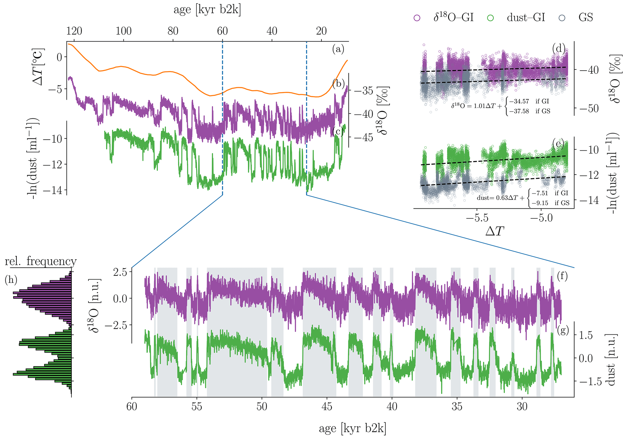
Figure 1(a) Global-mean surface temperature reconstruction for the last glacial interval as provided by Snyder (2016) and linearly interpolated to a 20-year temporal resolution. The reconstruction is based on a multi-proxy database which comprises over 20 000 sea surface temperature reconstructions from 59 marine sediment cores. The figure shows the anomaly with respect to modern climate (5–0 kyr b2k average; b2k: before 2000 CE). The 20-year mean of δ18O ratios (b) and accordingly resampled dust concentrations (c) from the NGRIP ice core in Greenland, from 122 kyr and 107 kyr to 10 kyr b2k (Rasmussen et al., 2014; Seierstad et al., 2014; Ruth et al., 2003). The dust data are given as the negative natural logarithm of the actual dust concentrations in order to facilitate visual comparison to the δ18O data. Panels (d) and (e) show the linear regressions of δ18O and dust onto the reconstructed global-mean surface temperatures (Snyder, 2016) from (a), carried out separately for Greenland stadials (GSs) and Greenland interstadials (GIs). Panels (f) and (g) show the same proxies as shown in (b) and (c) but at a higher resolution of 5 years (North Greenland Ice Core Projects members, 2004; Gkinis et al., 2014; Ruth et al., 2003) and over a shorter period from 59 to 27 kyr b2k. The analysis presented in this study was constrained to this section of the record. The two proxy time series in (f) and (g) have been detrended by removing the slow non-linear change induced by changes in the global background temperatures, based on the regressions from (d) and (e). The data were then binned to equidistant time resolution from the original 5 cm depth resolution. The grey shadings mark the GI intervals according to Rasmussen et al. (2014). Panel (h) shows the histograms of the two time series shown in (f) and (g), respectively. All data are shown on the GICC05 chronology (Vinther et al., 2006; Rasmussen et al., 2006; Andersen et al., 2006; Svensson et al., 2008).
The analysis presented here is based primarily on the joint δ18O ratio and dust concentration time series obtained by the North Greenland Ice Core Project (NGRIP) (North Greenland Ice Core Projects members, 2004; Ruth et al., 2003; Gkinis et al., 2014). From 1404.75–2426.00 m of depth in the NGRIP ice core, data are available for both proxies at a spatially equidistant resolution of 5 cm. This translates into non-equidistant temporal resolution ranging from sub-annual resolution at the end to ∼ 5 years at the beginning of the period, 59944.5–10276.4 years b2k, according to the Greenland Ice Core Chronology 2005 (GICC05), the common age–depth model for both proxies (Vinther et al., 2006; Rasmussen et al., 2006; Andersen et al., 2006; Svensson et al., 2008). Lower-resolution data (20-year means) (Rasmussen et al., 2014; Seierstad et al., 2014) reaching back to the last interglacial period (see Fig. 1) are only used for illustrative purposes but not for the analysis.
The ratio of stable water isotopes, expressed as δ18O values in units of permil, is a proxy for the site temperature at the time of precipitation, and hence the abrupt shifts present in the data qualitatively indicate the abrupt warming events over Greenland (Jouzel et al., 1997; Johnsen et al., 2001). The concentration of dust, i.e. the number of particles with a diameter above 1 µm mL−1, is commonly interpreted as a proxy for the state of the hemispheric atmospheric circulation (e.g. Fischer et al., 2007; Ruth et al., 2007; Schüpbach et al., 2018; Erhardt et al., 2019). More specifically, it is assumed to be controlled mostly by three factors (Fischer et al., 2007): first, by climatic conditions at the emission source, i.e. the dust storm activity over East Asian deserts preconditioned on generally dry regional climate; second, by the transport efficiency, which is affected by the strength and position of the polar jet stream; and third, the depositional process, which is mostly determined by local precipitation patterns. Correspondingly, the substantial changes in the dust concentrations across DO events are interpreted as large-scale reorganisations of the Northern Hemisphere's atmospheric circulation. Typically, atmospheric changes affecting the dust flux onto the Greenland ice sheet are accompanied by changes in the snow accumulation of opposite sign (e.g. Fischer et al., 2007). This enhances the corresponding change in the recorded dust particle concentration. However, for high-accumulation Greenland ice cores – such as NGRIP – the dust concentration changes still serve as a reliable indicator of atmospheric changes according to Fischer et al. (2007). Since the dust concentrations approximately follow an exponential distribution, we consider the negative natural logarithm of the dust concentration in order to emphasise the similarity to the δ18O time series. For ease of notation, we always use the term dust (or dust concentrations), although technically we refer to its negative natural logarithm.
In Fig. 1 we show the original low-resolution (b and c) and the pre-processed high-resolution data (f and g) together with corresponding histograms (h), also given in Fig. 3a. Clearly, two regimes can be visually distinguished: Greenland stadials are characterised by low δ18O ratios and high dust concentrations. Greenland interstadials (grey shading in panels f and g of Fig. 1) in general exhibit the reversed configuration besides a mild trend toward stadial conditions, which can be more or less pronounced during the individual interstadials. In our study, we use the categorisation of the climatic periods as presented by Rasmussen et al. (2014). The two-regime character of the time series translates into a bi-modal histogram of the dust data, as seen in Fig. 1h. In the case of the δ18O data, the stronger trend during interstadials and the higher relative noise amplitude mask a potential bi-modality, and the histogram appears unimodal. Notice that the somewhat counterintuitive combination of meta-stable distinct dynamical regimes and unimodal distributions of the associated variables has also been discussed in the context of atmospheric dynamics (Majda et al., 2006).
The analysis conducted in this work relies on the following assumptions and technical conditions:
- i.
The data-generating process is sufficiently time-homogeneous over the considered time period.
- ii.
The process is Markovian at the sampled temporal resolution.
- iii.
The data are equidistant in time.
- iv.
The relevant region of the state space is sampled sufficiently densely by the available data.
With regard to (i), a low-frequency influence of the background climate on the proxy values and on the frequency of DO events is evident (see Fig. 1), with suppressed DO variability during the coldest parts of the glacial and longer interstadials for its warmer parts (e.g. Rial and Saha, 2011; Roberts and Saha, 2017; Mitsui and Crucifix, 2017; Lohmann and Ditlevsen, 2018b; Boers et al., 2017, 2018). We therefore restrict our analysis to the period 59–27 kyr b2k, which is characterised by a fairly stable background climate and persistent co-variability between dust and δ18O (Boers et al., 2017). To remove the remaining influence of the background climate on the climate proxy records we remove a trend that is non-linear in time from both time series. This trend is obtained by linearly regressing the proxy data against reconstructed global-average surface temperatures (Snyder, 2016). Figure 1 illustrates the detrending scheme; due to the two-regime nature of the time series, a simple linear regression of the proxy variables onto the global-average surface temperatures would overestimate the temperature dependencies. Instead, we separate the data from Greenland stadials and Greenland interstadials and then minimise the quantity
once for x=δ18O and once for x, taken as dust concentrations. The optimisations yield optimal values for the parameters a, bGI, and bGS for dust and δ18O (see Fig. 1 panels d and e for δ18O and dust concentration, respectively). For a given time ti we write ti∈GS (GI) to indicate that ti falls into a stadial (interstadial) period. The index i runs over all data points, and N denotes the total number of data points. The resulting slope a is used to detrend the original data with respect to the time-dependent background temperature:
Subsequently, the detrended data are normalised by subtracting their respective means and dividing by their respective standard deviations. After the detrending, all stadial (or interstadial) periods exhibit almost the same level of values, which allows the data to be considered as the outcome of a time-homogeneous and long-term stationary process (compare Fig. 1f and g). As a consequence of the regime transitions the process is certainly not stationary on short timescales but only on timescales larger than typical DO cycle periods. Levelling out the differences between the recurring climate periods guarantees a sufficiently dense sampling of the relevant region of the state space (iv) and prevents a blurring of the drift reconstruction (i).
Table 1Unit root test of the detrended data. ADF refers to the augmented Dickey–Fuller test; ADF-GLS refers to the augmented Dickey–Fuller–GLS test. We reject the presence of a unit root in each of the time series at p<0.05.
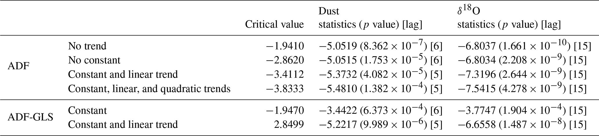
Stationarity tests provide further confirmation that the detrended data are free of any slow underlying trends: we have applied two separate tests to assess the stationarity of the detrended data on timescales beyond single DO cycles. These tests are the augmented Dickey–Fuller test (ADF) and the augmented Dickey–Fuller–GLS test (ADF-GLS). Both tests test the possibility of a unit root in the time series (null hypothesis). The alternative hypothesis is that the time series does not have a unit root; i.e. it is stationary. We can safely reject the presence of a unit root in each time series at p<0.05 (see Table 1).
There is a trade-off between conditions (i) and (iv) concerning the choice of the data window. While an even shorter window would assure time homogeneity of the dynamics with higher confidence, the sampling of the state space would become insufficiently sparse. The above choice (59–27 kyr b2k) guarantees a sufficient number of recurrences of the pre-processed two-dimensional trajectory to the relevant state space regions to perform statistical analysis. To obtain time-equidistant records (iii), the data are binned into temporally equidistant increments of 5 years.
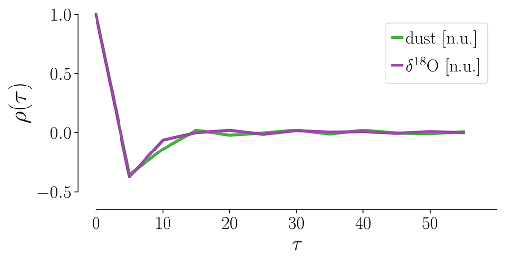
Figure 2Autocorrelation ρ(τ) of the increments Δxt of δ18O and dust records. Both records show a weak anti-correlation at the shortest lag τ=5 years and no correlation for τ>5 years. We thus consider the data Markovian.
The question of Markovianity (ii) is the most difficult to answer unambiguously. Here we draw on the following heuristic argument: the autocorrelation functions of the increments of both proxies shown in Fig. 2 exhibit weak anti-correlation at a shift of one time step, while correlations beyond this are negligible. Such a small level of correlation certainly rules out the notion that long-term memory effects played a major role in the emergence of the given time series. Bear in mind that this is a necessary yet not sufficient criterion to consider the data Markovian. For practical reasons, we refrained from further Markovianity tests.
Finally, further preconditions for our endeavour are the fact that the NGRIP record exhibits an exceptionally high resolution (iv) compared to other paleoclimate archives and that the two time series share the same time axis.
In this work, we treat the combined δ18O and dust record as a trajectory of a two-dimensional, time-homogeneous, and Markovian stochastic process of the form
where ξ denotes a general δ-correlated driving noise in the Itô sense. It may be state-dependent – i.e. explicitly depend on x – and contain discontinuous elements. No further specification is needed for the analysis presented here. The reconstruction of the two-dimensional drift F(x) is based on the Kramers–Moyal (KM) equation, which reads
in two dimensions, where denotes the probability for the system to assume the state (x1,x2) at time t, given that it was in the state at the time t′. The coefficients of the two-dimensional Kramers–Moyal equation can be estimated – analogously to the one-dimensional coefficients as explained in Tabar (2019) – from a realisation of a two-dimensional stochastic process . The terms D1,0(x) and D0,1(x) combine to the deterministic drift that governs the stochastic process:
In this work, we only consider the first-order KM coefficients. These are sufficient to uncover the deterministic non-linear features behind the stochastic data. Notice that we could formulate our method equally well in terms of the simpler Fokker–Planck equation (Risken and Frank, 1996). However, operating with the Fokker–Planck equation implicitly assumes that the stochastic process under investigation follows a Langevin equation in a strict sense; i.e. the noise term in Eq. (3) would be restricted to the case of Brownian motion. This conflicts with findings from ongoing research which indicate that the description of the driving noise ξ(t) as Brownian motion might not be valid (Rydin Gorjão et al., 2022). The use of the KM instead of the Fokker–Planck equation in this work aims at emphasising that ξ(t) might be more complex than Brownian motion and contain for example discontinuous elements. In principle, for a given stochastic process model, the higher-order KM coefficients can be used to estimate the corresponding noise parameters (see e.g. Anvari et al., 2016; Lehnertz et al., 2018; Rydin Gorjão et al., 2019; Tabar, 2019). However, this is not straightforward in two dimensions, and we deliberately refrain from an upfront selection of a process model in this work. Furthermore, a reliable estimate of higher-order coefficients in two dimensions is prevented by insufficient data density. A general derivation of the Kramers–Moyal equation can be found in Kramers (1940), Moyal (1949), Risken and Frank (1996), Gardiner (2009), and Tabar (2019).
In practice, in order to carry out the estimation of the first-order KM coefficients as defined in Eq. (4) we map each data point in the corresponding state space to a kernel density and then take a weighted average over all data points:
with .
Similar to selecting the number of bins in a histogram, when employing kernel density estimation with a Nadaraya–Watson estimator for the Kramers–Moyal coefficients Dm,n(x), one needs to select both a kernel and a bandwidth (Nadaraya, 1964; Watson, 1964; Lamouroux and Lehnertz, 2009). Firstly, the choice of the kernel is the choice of a function K(x) for the estimator , where h is the bandwidth at a point x
for a collection {xi} of n random variables. The kernel K(x) is normalised as and has a bandwidth h, such that (Rydin Gorjão et al., 2019; Tabar, 2019; Davis and Buffett, 2022). The bandwidth h is equivalent to the selection of the number of bins, except that binning in a histogram is always “placing numbers into non-overlapping boxes”. The optimal kernel is the commonly denoted Epanechnikov kernel (Epanechnikov, 1967), also used here for the analysis of the data:
Gaussian kernels are commonly used as well. Note that these require compact support in ; thus on a computer they require some sort of truncation (even in Fourier space, as the Gaussian shape remains unchanged).
The selection of an appropriate bandwidth h can be aided – unlike the selection of the number of bins – by Silverman's rule of thumb (Silverman, 1998), given by
where again σ2 is the variance of the time series. We note that the above formula for the ideal bandwidth has been developed for the estimation of the probability density function. As there is currently no consensus on the optimal kernel and bandwidth for the estimation of the KM coefficients, we employ an Epanechnikov kernel with bandwidth hs throughout our work.
All numerical analyses were performed with Python's NumPy (Harris et al., 2020), SciPy (Virtanen et al., 2020), and pandas (McKinney, 2010).
Kramers–Moyal analysis was performed with kramersmoyal (Rydin Gorjão and Meirinhos, 2019).
Figures were generated with Matplotlib (Hunter, 2007).
We first discuss the two drift components D1,0 and D0,1 (see Eq. 5) separately as functions of the two-dimensional space spanned by δ18O ratios and dust concentrations. In the component-wise analysis, the analysed component takes the role of a dynamical variable, while the respective other assumes the role of a controlling parameter. In this setting, corresponding nullclines can be computed, which reveals the bifurcation and stability structure of the two individual drift components. Intersections of the two components' nullclines yield fixed points of the coupled system, which are stable if both nullclines are stable at the intersection.
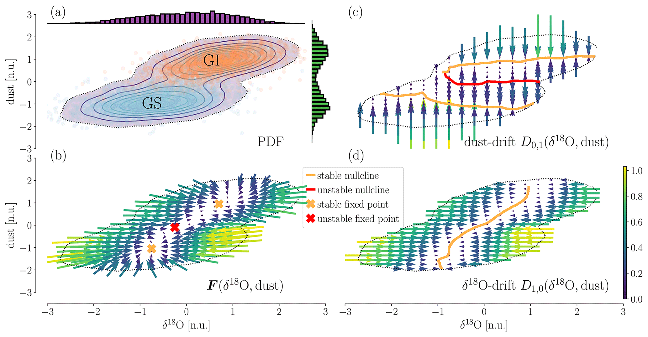
Figure 3Two-dimensional drift reconstruction. (a) PDF of the two-dimensional record, with projections onto both dimensions. Blue and orange dots represent the individual data points from Greenland stadials (GSs) and Greenland interstadials (GIs), respectively. Contour lines are obtained from a kernel density estimate of the data distribution. The dotted contour line indicates a chosen cutoff data density of >0.015 data points per pixel; regions in the state space with lower data density are not considered in the analysis. One pixel has the size of 0.015 × 0.015 in normalised units. (b) The reconstructed vector field F according to Eq. (5). Regions of convergence are apparent and correspond to the GI and GS states of the record. (c) The dust component D0,1 of the reconstructed drift. The dust's nullcline exhibits an S shape, with two stable branches (orange) and an unstable one in between (red), indicative of a double-fold bifurcation with δ18O as a control parameter. (d) The δ18O component D1,0 of the reconstructed drift. Here, the nullcline is comprised of a single stable branch (orange). The position of the δ18O fixed point varies with the value of the dust. Fixed points of the coupled system are given by the intersections of the two components' nullclines, marked with an X in panel (b).
4.1 Double-fold bifurcation of the dust
The estimated dust drift is displayed in Fig. 3c. This coefficient dictates the deterministic motion of the system along the dust direction; therein the δ18O ratio takes the role of the controlling parameter. We can trace the nullcline's branches, which take a general “S” shape as we vary δ18O. Hence, depending on the value of δ18O, there is either one or three fixed points for the motion along the dust direction: for approximately δ18O , there is one stable fixed point; for approximately O <0.9, there are three fixed points, two stable ones and an unstable one between them; for approximately δ18O >0.9, there is again just one stable fixed point. In fact, the merger of the nullcline's lower stable branch and unstable branch is not fully captured by the reconstruction due to too-low data density in the corresponding region (see Fig. 3c). With the position of these stable fixed points depending continuously on δ18O ratios, we find here the characteristic form of a double-fold bifurcation, in which δ18O takes the role of a control parameter.
The dust nullclines' structure supports the possibility for abrupt transitions in two ways: either random fluctuations move the system across the unstable branch (if present, depending on the value of the control parameter), or the control parameter, in this case δ18O, crosses a bifurcation point, and the currently attracting stable branch merges with the unstable branch. In both cases, the system will transition fairly abruptly to the alternative stable branch. A rate-induced transition seems implausible in this case since the unstable branch is approximately constant with respect to a change in the control parameter (i.e. δ18O). Thus, a crossing of the unstable branch by means of a rapid shift in δ18O seems highly unlikely.
4.2 Coupling of the δ18O drift with the dust
We now focus on the reconstructed drift of the δ18O ratios (Fig. 3d). Its nullcline appears to be an explicit function of the dust; i.e. for each value of dust concentration there is a single stable fixed point along the δ18O dimension. The position of the fixed point changes with the value for dust in a continuous manner, with a high rate of change for intermediate dust values and a small change for more extreme dust values. These findings suggest that δ18O follows a mono-stable process whose fixed point is subject to change in response to an “external control” imposed by the dust.
4.3 Combined two-dimensional drift
Figure 3b shows the two-dimensional drift field F(δ18O,dust) of the coupled system given by Eq. (5). The two fixed points which arise from the intersections of the dust nullcline's stable branches with the δ18O stable nullcline fall well within the regions of the state space associated with Greenland stadials and interstadials, respectively. The stable regime (δ18O , dust ) can be identified with Greenland stadials, while the stable regime (δ18O ∼0.5, dust ∼1) corresponds to Greenland interstadials. Similarly, we can locate an unstable fixed point roughly in between the two observed stabled fixed points of the coupled system. Judging from Fig. 3b the unstable fixed point resembles a saddle with a convergent drift along the δ18O direction and divergence along the connection line between the two stable fixed points. The system's bistability is inherited from the dust's drift and is not enshrined in the δ18O ratios. As mentioned previously, Fig. 3b suggests that – starting from a stable fixed point – perturbations along the δ18O direction will not entail state transitions but instead simply decay until the system reaches the δ18O nullcline again. In contrast, perturbations along the dust direction may shift the system into the other respective basin of attraction.
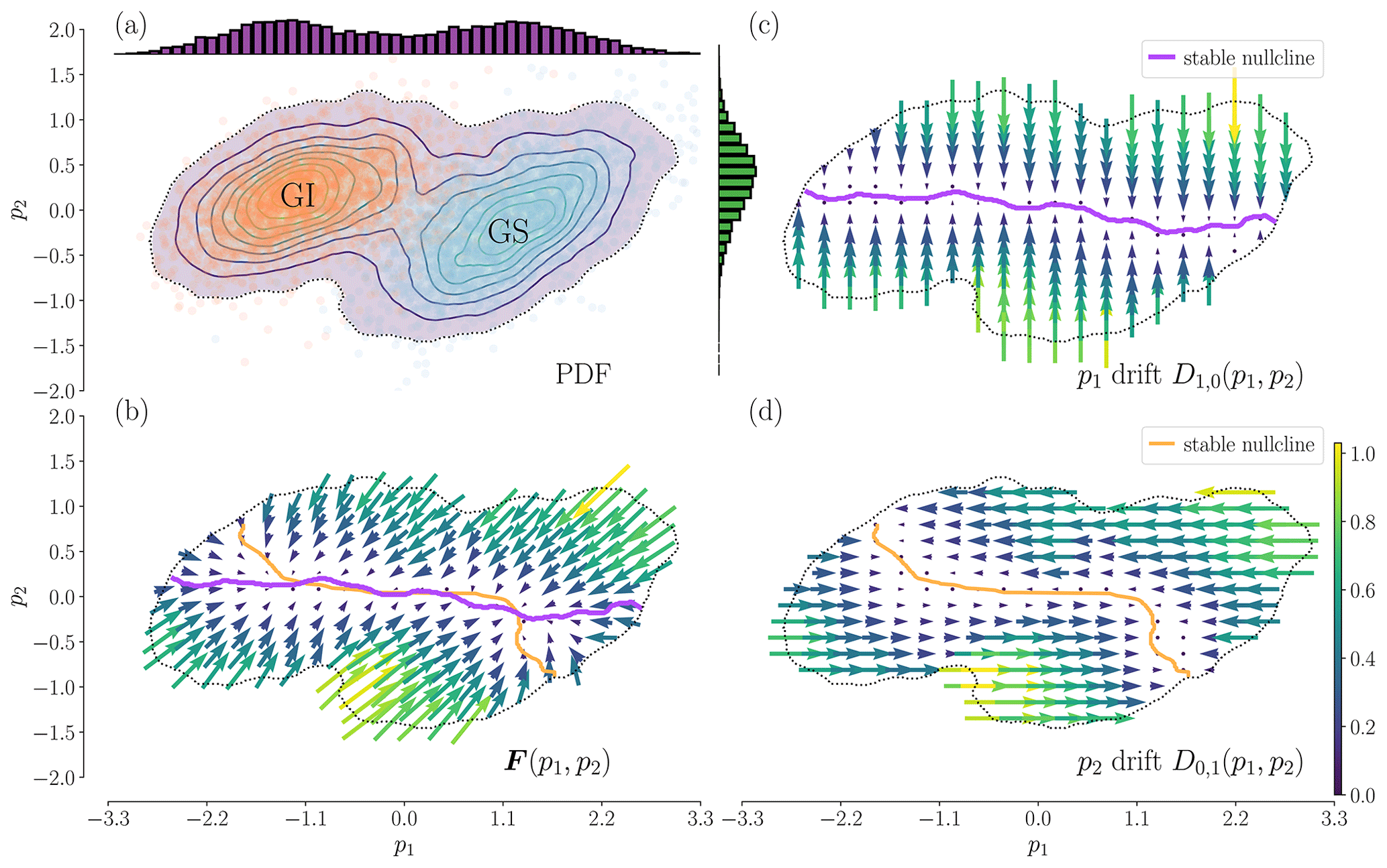
Figure 4Redrawing of Fig. 3 in a rotated state space. The variables p1 and p2 represent the rotated time series, onto which the same KM analysis is performed as before. We can observe that even in this rotated setting we cannot disregard the coupling of the two variables. The doubled-fold structure is occluded by the rotation (see drift of the variable p1 in panel c). The drift of p2 remains dependent on p1 (see panel d). We can thus conclude that the observed coupling is not an artefact of the initial state space used and is an intrinsic characteristic of the two proxies.
4.4 Rotation of the state space and the presence of a non-negligible interplay of the dust and δ18O
Above we argue for the existence of a double-fold bifurcation in the dust variable. In order to show that the coupling of the dust and δ18O is not a spurious result of the initial state space, we conduct an analogue analysis using a rotated state space. To rotate the state space we employ principal component analysis and obtain a new set of variables , with , where U is given by
In Fig. 4 we redraw Fig. 3 in the rotated state space; we observe that (i) the nullcline of p1 is now almost independent of p2, and (ii) the p2 nullcline is still strongly dependent on p1, while none of the rotated variables show any bifurcation. Overall, the dynamics of the dust–δ18O can be explained as we introduce in Sect. 4.2, with two basins of attraction being separated by a saddle. In particular, the assessment of the drift in the rotated state space shows that the data cannot be described by a simple two-dimensional double-well potential with two axes of symmetry and decoupled dynamics along them.
We use the two-dimensional Kramers–Moyal equation to investigate the deterministic drift of the combined dust and δ18O record from the NGRIP ice core for the time interval 59–27 kyr b2k, which exhibits pronounced DO variability. The reconstructed stability structure with two basins of attraction and a separating saddle is consistent with the regime switches observed simultaneously in both components of the record: in the δ18O–dust plane, the basins of attraction are located such that a transition from one to the other entails a change in both components. However, the analysis of the vector field (Fig. 3b) does not indicate any clear paths the system takes in order to transition between stadial and interstadial states. The shape of the nullclines can, in principle, allow for a situation where a perturbation along the δ18O direction pushes the dust across its bifurcation point, triggering a transition of the dust, which in turn stabilises the δ18O perturbation. The combined drift F(x1,x2), however, exhibits strong restoring forces along the δ18O direction, which render this mechanism rather implausible. Viewed from either stable fixed point, perturbations along the dust direction could in contrast push the system across the basin boundary relatively easily. Certainly, a combination of noise along both directions may also be able to drive the system across the region of weak divergence that separates the two attractors. We note that the mild relaxation that is typical for Greenland interstadials cannot be explained by the results of this analysis alone. As mentioned previously, an estimation of the KM coefficients for the individual, univariate δ18O and dust time series indicates that at least the δ18O noise comprises non-Gaussian and potentially discontinuous components, which could play a central role with respect to the transition between the two identified stable states of the drift (Rydin Gorjão et al., 2022). However, there remain discrepancies to be reconciled in the analysis of the higher-order KM coefficients of the individual δ18O and dust time series such that arguments about the role of non-Gaussian noise in the regime transitions remain speculative at this point. Ideally, higher-order KM coefficients should be computed for the two-dimensional record; however, this is prevented by the low data resolution.
In the following, we discuss how the results presented here relate to the findings of previous studies. An important branch of research around DO events draws on low-dimensional conceptional modelling and, related to that, inverse modelling approaches with model equations being fitted to ice core data. Many of these studies build on stochastic differential equations and in particular on Langevin-type equations. Our study follows the same key paradigm, regarding the paleoclimate record as the realisation of a stochastic process. However, as far as we know, it is the first study to assess the two-dimensional drift non-parametrically in the δ18O–dust plane.
For the period investigated here Livina et al. (2010) attested bistability to both the δ18O and the dust component individually by fitting a Langevin process to a 20-year-mean version of the NGRIP record. Later Kwasniok (2013) and Lohmann and Ditlevsen (2018a) showed – using techniques from Bayesian model inference – that a two-dimensional relaxation oscillator model outperforms a simple double-well potential in terms of simulating the NGRIP δ18O record. Such a relaxation oscillation still relies on a fundamental bistability in the variable that is identified with δ18O ratios. A physical interpretation for a FitzHugh–Nagumo-type DO model is provided by Vettoretti et al. (2022).
Our results contradict the interpretation that δ18O ratios and therewith Greenland temperatures bear an intrinsic bistability. In the two-dimensional setting, the apparent two-regime nature of the δ18O record can be explained by the control that the dust exerts on the δ18O fixed points and the corresponding location of the two stable fixed points in the two-dimensional drift. Since we find the bistability of the reconstructed coupled system rooted in the dust, our analysis suggests that the atmosphere may have played a more active role in stabilising the two regimes that dominated the last glacial's Northern Hemisphere climate than many AMOC-based explanations of the DO variability suggest (Ganopolski and Rahmstorf, 2002; Clark et al., 2002; Vettoretti and Peltier, 2018; Li and Born, 2019; Menviel et al., 2020). Similarly, the observation that dust perturbations may induce state transitions may be seen as a hint that random perturbation of the atmospheric circulation can trigger DO events as proposed by, for example, Kleppin et al. (2015). In this regard, it should be noted that a multistability of the latitudinal jet stream position has been suggested – although in a somewhat different setting and sense – based on an investigation of reanalysis data of modern climate (Woollings et al., 2010). In contrast, one would not expect two distinct stable Greenland temperature regimes with all controlling factors kept fixed. This is in line with the bistability of the dust drift and the mono-stable δ18O drift revealed in our analysis.
Clearly, the state space spanned by δ18O and dust is a very particular one. On the one hand, the interpretation of the two proxies as indicators of Greenland temperatures and the hemispheric circulation state of the atmosphere bears qualitative uncertainties and should certainly not be considered a one-to-one mapping. On the other hand, other climate subsystems not directly represented in the data analysed here, like the AMOC for example, are likely to have played an important role in the physics of DO variability as well. Even if δ18O ratios and dust concentrations were to exclusively represent Greenland temperatures and the atmospheric circulation state, the recorded climate variables were certainly highly entangled with other climate variables such as the AMOC strength, the Nordic Sea's and North Atlantic's sea ice cover, or potentially North American ice sheet height (e.g. Menviel et al., 2020; Li and Born, 2019; Boers et al., 2018; Zhang et al., 2014; Dokken et al., 2013). In our analysis, such couplings are subsumed in the δ-correlated noise term ξ – an approach which may rightfully be criticised to be overly simplistic. However, given the lack of climate proxy records that jointly represent more DO-relevant components of the climate system on the same chronology, the chosen method reasonably complements existing data-driven investigations of DO variability. For example Boers et al. (2017) similarly examined the dynamical features of the combined δ18O–dust record. They proposed a third-order polynomial two-dimensional drift in combination with a non-Markovian term and Gaussian white noise to model the coupled dynamics. While our approach is limited to a Markovian setting, it allows for more general forms of drift (and noise). Being non-parametric, it does not rely on prior model assumptions in this regard. It is not per se clear how the couplings to “hidden” climate variables (i.e. those not represented by the analysed proxy record) influence the presented drift reconstruction, and there is certainly a risk of missing a relevant part of the dynamics.
We have analysed the records of δ18O ratios and dust concentrations from the NGRIP ice core from a data-driven perspective. The central point of our study was to examine the stability configuration of the coupled δ18O–dust process by reconstructing its two-dimensional drift. Our findings indicate a mono-stable δ18O drift whose fixed point's position is an explicit function of the dust. The dust variable, in contrast, seems to undergo a double-fold bifurcation parameterised by δ18O, with a change from a single (stable) fixed point to three fixed points (two stable, one unstable) and again to a single (stable) fixed point, from small to large values of the δ18O ratio. Together, the drift components yield two stable fixed points in the coupled system surrounded by convergent regions in the δ18O–dust state space, in agreement with the two-regime nature of the coupled record. Judging from the reconstructed drift, perturbations along the dust dimension are more likely to trigger a state transition, which points to an active role of atmospheric circulation in DO variability.
Importantly, our findings question the prevailing interpretation of the two regimes observed in the isolated δ18O record as the direct signature of an intrinsic bistability. Such an intrinsic bistability can be confirmed only for the dust variable. Regarding δ18O ratios as a direct measure of the local temperature, it seems plausible that not the temperature itself is bistable but rather that the bistability is enshrined in another climate variable – or at least a regional-scale climate process or a combination of processes – that drives Greenland temperatures. The apparent two-regime nature of the δ18O record would thus only be inherited from the actual bistability of other processes. This may be the atmospheric circulation as represented by the dust proxy or another external driver not directly represented by the analysed data.
Similar investigations to ours should be applied to other pairs of Greenland proxies to investigate the corresponding two-dimensional drift. Finally, our study underlines the need for higher-resolution data, as the scarcity of data points is a limiting factor for the quality of non-parametric estimates of the KM coefficients.
The code to reproduce the analysis and all figures is available at https://doi.org/10.5281/zenodo.7898825 (Kriechers, 2023) or upon request to the corresponding author.
All ice core data were obtained from the website of the Niels Bohr Institute of the University of Copenhagen https://www.iceandclimate.nbi.ku.dk/data (Niels Bohr Institute, 2023). The original measurements of δ18O ratios and dust concentrations go back to North Greenland Ice Core Projects members (2004) and Ruth et al. (2003), respectively. The 5 cm resolution δ18O ratio and dust concentration data together with corresponding GICC05 ages used for this study can be downloaded from https://www.iceandclimate.nbi.ku.dk/data/NGRIP_d18O_and_dust_5cm.xls (last access: 4 May 2023). The δ18O data shown in Fig. 1 with 20-year resolution that cover the period 122–10 kyr b2k are available from https://www.iceandclimate.nbi.ku.dk/data/GICC05modelext_GRIP_and_GISP2_and_resampled_data_series_Seierstad_et_al._2014_version_10Dec2014-2.xlsx (last access: 4 May 2023) likewise hosted on website indicated above (Niels Bohr Institute, 2023). They were published in conjunction with the work by Rasmussen et al. (2014) and Seierstad et al. (2014). The corresponding dust data, also shown in Fig. 1 and covering the period 108–10 kyr b2k, is due to Ruth et al. (2003) and can be retrieved from the website of the Niels Bohr Institute (2023) (https://www.iceandclimate.nbi.ku.dk/data/NGRIP_dust_on_GICC05_20y_december2014.txt, last access: 4 May 2023). The global-average surface temperature reconstructions is available as a supplement to Snyder (2016) and the direct link for the download is https://static-content.springer.com/esm/art%3A10.1038%2Fnature19798/MediaObjects/41586_2016_BFnature19798_MOESM258_ESM.xlsx (last access: 4 May 2023).
KR and LRG designed the study with contributions from all authors. KR and LRG conducted the numerical analysis. KR and LRG wrote the paper with contributions from all authors.
The contact author has declared that none of the authors has any competing interests.
Publisher’s note: Copernicus Publications remains neutral with regard to jurisdictional claims in published maps and institutional affiliations.
Leonardo Rydin Gorjão and Dirk Witthaut gratefully acknowledge support from the Helmholtz Association via the grant “Uncertainty Quantification – From Data to Reliable Knowledge” (UQ; grant agreement no. ZT-I-0029). This work was performed by Leonardo Rydin Gorjão as part of the Helmholtz School for Data Science in Life, Earth and Energy (HDS-LEE). Niklas Boers acknowledges funding from the Volkswagen Foundation. This is TiPES contribution no. 162; the “Tipping Points in the Earth System” (TiPES) project has received funding from the European Union's Horizon 2020 research and innovation programme under grant agreement no. 820970.
This research has received funding from the European Union's Horizon 2020 research and
innovation programme (TiPES; grant no. 820970), the Helmholtz-Gemeinschaft
(grant nos. ZT-I-0029 and HIDDS-0004), and the Volkswagen Foundation.
This work was supported by the Technical University of Munich (TUM) in the framework of the Open Access Publishing Program.
This paper was edited by Valerio Lucarini and reviewed by Peter Ditlevsen, Tamas Bodai, Christian Franzke, Mohammed Reza Rahimi Tabar, and one anonymous referee.
Andersen, K. K., Svensson, A., Johnsen, S. J., Rasmussen, S. O., Bigler, M., Röthlisberger, R., Ruth, U., Siggaard-Andersen, M. L., Peder Steffensen, J., Dahl-Jensen, D., Vinther, B. M., and Clausen, H. B.: The Greenland Ice Core Chronology 2005, 15–42 ka, Part 1: constructing the time scale, Quaternary Sci. Rev., 25, 3246–3257, https://doi.org/10.1016/j.quascirev.2006.08.002, 2006. a, b
Anvari, M., Tabar, M. R. R., Peinke, J., and Lehnertz, K.: Disentangling the stochastic behavior of complex time series, Sci. Rep., 6, 35435, https://doi.org/10.1038/srep35435, 2016. a
Armstrong McKay, D. I., Staal, A., Abrams, J. F., Winkelmann, R., Sakschewski, B., Loriani, S., Fetzer, I., Cornell, S. E., Rockström, J., and Lenton, T. M.: Exceeding 1.5 ∘C global warming could trigger multiple climate tipping points, Science, 377, eabn7950, https://doi.org/10.1126/science.abn7950, 2022. a
Ashwin, P., Wieczorek, S., Vitolo, R., and Cox, P.: Tipping points in open systems: Bifurcation, noise-induced and rate-dependent examples in the climate system, Philos. T. R. Soc. A, 370, 1166–1184, https://doi.org/10.1098/rsta.2011.0306, 2012. a
Boers, N.: Observation-based early-warning signals for a collapse of the Atlantic Meridional Overturning Circulation, Nat. Clim. Change, 11, 680–688, https://doi.org/10.1038/s41558-021-01097-4, 2021. a, b
Boers, N. and Rypdal, M.: Critical slowing down suggests that the western Greenland Ice Sheet is close to a tipping point, P. Natl. Acad. Sci. USA, 118, e2024192118, https://doi.org/10.1073/pnas.2024192118, 2021. a, b
Boers, N., Chekroun, M. D., Liu, H., Kondrashov, D., Rousseau, D.-D., Svensson, A., Bigler, M., and Ghil, M.: Inverse stochastic–dynamic models for high-resolution Greenland ice core records, Earth Syst. Dynam., 8, 1171–1190, https://doi.org/10.5194/esd-8-1171-2017, 2017. a, b, c, d, e
Boers, N., Ghil, M., and Rousseau, D. D.: Ocean circulation, ice shelf, and sea ice interactions explain Dansgaard–Oeschger cycles, P. Natl. Acad. Sci. USA, 115, E11005–E11014, https://doi.org/10.1073/pnas.1802573115, 2018. a, b, c
Boers, N., Ghil, M., and Stocker, T. F.: Theoretical and paleoclimatic evidence for abrupt transitions in the Earth system, Environ. Res. Lett., 17, 093006, https://doi.org/10.1088/1748-9326/ac8944, 2022. a
Boulton, C. A., Allison, L. C., and Lenton, T. M.: Early warning signals of Atlantic Meridional Overturning Circulation collapse in a fully coupled climate model, Nat. Commun., 5, 5752, https://doi.org/10.1038/ncomms6752, 2014. a
Boulton, C. A., Lenton, T. M., and Boers, N.: Pronounced loss of Amazon rainforest resilience since the early 2000s, Nat. Clim. Change, 12, 271–278, https://doi.org/10.1038/s41558-022-01287-8, 2022. a
Brovkin, V., Brook, E., Williams, J. W., Bathiany, S., Lenton, T. M., Barton, M., DeConto, R. M., Donges, J. F., Ganopolski, A., McManus, J., Praetorius, S., de Vernal, A., Abe-Ouchi, A., Cheng, H., Claussen, M., Crucifix, M., Gallopín, G., Iglesias, V., Kaufman, D. S., Kleinen, T., Lambert, F., van der Leeuw, S., Liddy, H., Loutre, M.-f., McGee, D., Rehfeld, K., Rhodes, R., Seddon, A. W. R., Trauth, M. H., Vanderveken, L., and Yu, Z.: Past abrupt changes, tipping points and cascading impacts in the Earth system, Nat. Geosci., 14, 550–558, https://doi.org/10.1038/s41561-021-00790-5, 2021. a
Cheng, H., Sinha, A., Cruz, F. W., Wang, X., Edwards, R. L., D'Horta, F. M., Ribas, C. C., Vuille, M., Stott, L. D., and Auler, A. S.: Climate change patterns in Amazonia and biodiversity, Nat. Commun., 4, 1411, https://doi.org/10.1038/ncomms2415, 2013. a
Clark, P. U., Pisias, N. G., Stocker, T. F., and Weaver, A. J.: The role of the thermohaline circulation in abrupt climate change, Nature, 415, 863–869, https://doi.org/10.1038/415863a, 2002. a
Corrick, E. C., Drysdale, R. N., Hellstrom, J. C., Capron, E., Rasmussen, S. O., Zhang, X., Fleitmann, D., Couchoud, I., Wolff, E., and Monsoon, S. A.: Synchronous timing of abrupt climate changes during the last glacial period, Science, 369, 963–969, https://doi.org/10.1126/science.aay5538, 2020. a
Dansgaard, W., Clausen, H. B., Gundestrup, N., Hammer, C. U., Johnsen, S. F., Kristinsdottir, P. M., and Reeh, N.: A New Greenland Deep Ice Core, Science, 218, 1273–1278, https://doi.org/10.1126/science.218.4579.1273, 1982. a
Dansgaard, W., Johnsen, S., Clausen, H., Dahl-Jensen, D., Gundestrup, N., Hammer, C., and Oeschger, H.: North Atlantic Climatic Oscillations Revealed by Deep Greenland Ice Cores, American Geophysical Union, 29, 288–298, https://doi.org/10.1029/GM029p0288, 1984. a
Dansgaard, W., Johnsen, S. J., Clausen, H. B., Dahl-Jensen, D., Gundestrup, N. S., Hammer, C. U., Hvidberg, C. S., Steffensen, J. P., Sveinbjörnsdottir, A. E., Jouzel, J., and Bond, G.: Evidence for general instability of past climate from a 250-kyr ice-core record, Nature, 364, 218–220, https://doi.org/10.1038/364218a0, 1993. a
Davis, W. and Buffett, B.: Estimation of drift and diffusion functions from unevenly sampled time-series data, Phys. Rev. E, 106, 014140, https://doi.org/10.1103/PhysRevE.106.014140, 2022. a
Ditlevsen, P. D.: Observation of α-stable noise induced millennial climate changes from an ice-core record, Geophys. Res. Lett., 26, 1441–1444, https://doi.org/10.1029/1999GL900252, 1999. a, b
Dokken, T. M., Nisancioglu, K. H., Li, C., Battisti, D. S., and Kissel, C.: Dansgaard–Oeschger cycles: Interactions between ocean and sea ice intrinsic to the Nordic seas, Paleoceanography, 28, 491–502, https://doi.org/10.1002/palo.20042, 2013. a
Epanechnikov, V. A.: Non-Parametric Estimation of a Multivariate Probability Density, Theory Probab. Appl., 14, 153–158, https://doi.org/10.1137/1114019, 1967. a
EPICA Community Members: One-to-one coupling of glacial climate variability in Greenland and Antarctica, Nature, 444, 5–8, https://doi.org/10.1038/nature05301, 2006. a
Erhardt, T., Capron, E., Olander Rasmussen, S., Schüpbach, S., Bigler, M., Adolphi, F., and Fischer, H.: Decadal-scale progression of the onset of Dansgaard–Oeschger warming events, Clim. Past, 15, 811–825, https://doi.org/10.5194/cp-15-811-2019, 2019. a
Fischer, H., Siggaard-Andersen, M. L., Ruth, U., Röthlisberger, R., and Wolff, E.: Glacial/interglacial changes in mineral dust and sea-salt records in polar ice cores: Sources, transport, and deposition, Rev. Geophys., 45, 1–26, https://doi.org/10.1029/2005RG000192, 2007. a, b, c, d
Ganopolski, A. and Rahmstorf, S.: Abrupt Glacial Climate Changes due to Stochastic Resonance, Phys. Rev. Lett., 88, 038501, https://doi.org/10.1103/PhysRevLett.88.038501, 2002. a
Gardiner, C.: Stochastic Methods: A Handbook for the Natural and Social Sciences, Springer-Verlag Berlin Heidelberg, 4th Edn., ISBN 3-540-15607-0, 2009. a
Ghil, M.: Steady-State Solutions of a Diffusive Energy-Balance Climate Model and Their Stability, Tech. Rep. IMM410, Courant Institute of Mathematical Sciences, New York University, New York, https://ntrs.nasa.gov/api/citations/19750014903/downloads/19750014903.pdf (last access: 28 April 2023), 1975. a
Gkinis, V., Simonsen, S. B., Buchardt, S. L., White, J. W., and Vinther, B. M.: Water isotope diffusion rates from the NorthGRIP ice core for the last 16,000 years – Glaciological and paleoclimatic implications, Earth Planet. Sc. Lett., 405, 132–141, https://doi.org/10.1016/j.epsl.2014.08.022, 2014. a, b, c
Gottschalk, J., Skinner, L. C., Misra, S., Waelbroeck, C., Menviel, L., and Timmermann, A.: Abrupt changes in the southern extent of North Atlantic Deep Water during Dansgaard-Oeschger events, Nat. Geosci., 8, 950–954, https://doi.org/10.1038/ngeo2558, 2015. a
Harris, C. R., Millman, K. J., van der Walt, S. J., Gommers, R., Virtanen, P., Cournapeau, D., Wieser, E., Taylor, J., Berg, S., Smith, N. J., Kern, R., Picus, M., Hoyer, S., van Kerkwijk, M. H., Brett, M., Haldane, A., Fernández del Río, J., Wiebe, M., Peterson, Pearu andGérard-Marchant, P., Sheppard, K., Reddy, T., Weckesser, W., Abbasi, H., Gohlke, C., and Oliphant, T. E.: Array programming with NumPy, Nature, 585, 357–362, https://doi.org/10.1038/s41586-020-2649-2, 2020. a
Henry, L. G., McManus, J. F., Curry, W. B., Roberts, N. L., Piotrowski, A. M., and Keigwin, L. D.: North Atlantic ocean circulation and abrupt climate change during the last glaciation, Science, 353, 470–474, https://doi.org/10.1126/science.aaf5529, 2016. a
Hunter, J. D.: Matplotlib: A 2D Graphics Environment, Comput. Sci. Eng., 9, 90–95, https://doi.org/10.1109/MCSE.2007.55, 2007. a
Johnsen, S. J., Clausen, H. B., Dansgaard, W., Fuhrer, K., Gundestrup, N., Hammer, C. U., Iversen, P., Jouzel, J., Stauffer, B., and Steffensen, J.: Irregular glacial interstadials recorded in a new Greenland ice core, Nature, 359, 311–313, https://doi.org/10.1038/359311a0, 1992. a
Johnsen, S. J., Dahl-Jensen, D., Gundestrup, N., Steffensen, J. P., Clausen, H. B., Miller, H., Masson-Delmotte, V., Sveinbjörnsdottir, A. E., and White, J.: Oxygen isotope and palaeotemperature records from six Greenland ice-core stations: Camp Century, Dye-3, GRIP, GISP2, Renland and NorthGRIP, J. Quaternary Sci., 16, 299–307, https://doi.org/10.1002/jqs.622, 2001. a
Jouzel, J., Alley, R. B., Cuffey, K. M., Dansgaard, W., Grootes, P., Hoffmann, G., Johnsen, S. J., Koster, R. D., Peel, D., Shuman, C. A., Stievenard, M., Stuiver, M., and White, J.: Validity of the temperature reconstruction from water isotopes in ice cores, J. Geophys. Res.-Ocean., 102, 26471–26487, https://doi.org/10.1029/97JC01283, 1997. a
Kanner, L. C., Burns, S. J., Cheng, H., and Edwards, R. L.: High-Latitude Forcing of the South American Summer Monsoon During the Last Glacial, Science, 335, 570–573, https://doi.org/10.1126/science.1213397, 2012. a
Kindler, P., Guillevic, M., Baumgartner, M., Schwander, J., Landais, A., and Leuenberger, M.: Temperature reconstruction from 10 to 120 kyr b2k from the NGRIP ice core, Clim. Past, 10, 887–902, https://doi.org/10.5194/cp-10-887-2014, 2014. a
Kleppin, H., Jochum, M., Otto-Bliesner, B., Shields, C. A., and Yeager, S.: Stochastic atmospheric forcing as a cause of Greenland climate transitions, J. Clim., 28, 7741–7763, https://doi.org/10.1175/JCLI-D-14-00728.1, 2015. a
Kondrashov, D., Kravtsov, S., Robertson, A. W., and Ghil, M.: A Hierarchy of Data-Based ENSO Models, J. Clim., 18, 4425–4444, https://doi.org/10.1175/JCLI3567.1, 2005. a
Kondrashov, D., Chekroun, M. D., and Ghil, M.: Data-driven non-Markovian closure models, Physica D, 297, 33–55, https://doi.org/10.1016/j.physd.2014.12.005, 2015. a
Kramers, H. A.: Brownian motion in a field of force and the diffusion model of chemical reactions, Physica, 7, 284–304, https://doi.org/10.1016/S0031-8914(40)90098-2, 1940. a, b
Kriechers, R.: kriechers/esd-2021-95: esd-2021-95 (Version v1), Zenodo [code], https://doi.org/10.5281/zenodo.7898825, 2023. a
Kwasniok, F.: Analysis and modelling of glacial climate transitions using simple dynamical systems, Philos. T. R. Soc. A, 371, 20110472, https://doi.org/10.1098/rsta.2011.0472, 2013. a, b, c, d
Lamouroux, D. and Lehnertz, K.: Kernel-based regression of drift and diffusion coefficients of stochastic processes, Phys. Lett. A, 373, 3507–3512, https://doi.org/10.1016/j.physleta.2009.07.073, 2009. a
Lehnertz, K., Zabawa, L., and Tabar, M. R. R.: Characterizing abrupt transitions in stochastic dynamics, New J. Phys., 20, 113043, https://doi.org/10.1088/1367-2630/aaf0d7, 2018. a
Lenton, T., Held, H., Kriegler, E., Hall, J. W., Lucht, W., Rahmstorf, S., and Schellnhuber, H. J.: Tipping elements in the Earth's climate system, P. Natl. Acad. Sci. USA, 105, 1786–1793, https://doi.org/10.1073/pnas.0705414105, 2008. a
Lenton, T. M. and Schellnhuber, H. J.: Tipping the Scales, Nat. Clim. Change, 1, 97–98, https://doi.org/10.1038/climate.2007.65, 2007. a
Li, C. and Born, A.: Coupled atmosphere-ice-ocean dynamics in Dansgaard–Oeschger events, Quaternary Sci. Rev., 203, 1–20, https://doi.org/10.1016/j.quascirev.2018.10.031, 2019. a, b
Li, T.-Y., Han, L.-Y., Cheng, H., Edwards, R. L., Shen, C.-C., Li, H.-C., Li, J.-Y., Huang, C.-X., Zhang, T.-T., and Zhao, X.: Evolution of the Asian summer monsoon during Dansgaard/Oeschger events 13–17 recorded in a stalagmite constrained by high-precision chronology from southwest China, Quaternary Res., 88, 121–128, https://doi.org/10.1017/qua.2017.22, 2017. a
Livina, V. N., Kwasniok, F., and Lenton, T. M.: Potential analysis reveals changing number of climate states during the last 60 kyr, Clim. Past, 6, 77–82, https://doi.org/10.5194/cp-6-77-2010, 2010. a, b, c
Lohmann, J. and Ditlevsen, P. D.: A consistent statistical model selection for abrupt glacial climate changes, Clim. Dynam., 52, 6411–6426, https://doi.org/10.1007/s00382-018-4519-2, 2018a. a, b, c, d
Lohmann, J. and Ditlevsen, P. D.: Random and externally controlled occurrences of Dansgaard–Oeschger events, Clim. Past, 14, 609–617, https://doi.org/10.5194/cp-14-609-2018, 2018b. a
Lynch-Stieglitz, J.: The Atlantic Meridional Overturning Circulation and Abrupt Climate Change, Annu. Rev. Mar. Sci., 9, 83–104, https://doi.org/10.1146/annurev-marine-010816-060415, 2017. a, b
Majda, A. J., Franzke, C. L., Fischer, A., and Crommelin, D. T.: Distinct metastable atmospheric regimes despite nearly Gaussian statistics: A paradigm model, P. Natl. Acad. Sci. USA, 103, 8309–8314, https://doi.org/10.1073/pnas.0602641103, 2006. a
McKinney, W.: Data Structures for Statistical Computing in Python, in: Proceedings of the 9th Python in Science Conference, 28 June–3 July 2010, Austin, Texas, edited by: van der Walt, S. and Millman, J., 56–61, https://doi.org/10.25080/Majora-92bf1922-00a, 2010. a
Menviel, L. C., Skinner, L. C., Tarasov, L., and Tzedakis, P. C.: An ice–climate oscillatory framework for Dansgaard–Oeschger cycles, Nat. Rev. Earth Environ., 1, 677–693, https://doi.org/10.1038/s43017-020-00106-y, 2020. a, b, c, d
Mitsui, T. and Crucifix, M.: Influence of external forcings on abrupt millennial-scale climate changes: a statistical modelling study, Clim. Dynam., 48, 2729–2749, https://doi.org/10.1007/s00382-016-3235-z, 2017. a, b, c
Moyal, J. E.: Stochastic processes and statistical physics, J. R. Stat. Soc. Ser. B, 11, 150–210, 1949. a, b
Nadaraya, E. A.: On Estimating Regression, Theor. Probab. Appl., 9, 141–142, https://doi.org/10.1137/1109020, 1964. a
Niels Bohr Institute: Center for Ice and Climate – Data icesamples and software, University of Copenhagen, Copenhagen, Denmark, [data sets], https://www.iceandclimate.nbi.ku.dk/data/ and https://www.iceandclimate.nbi.ku.dk/data/NGRIP_dust_on_GICC05_20y_december2014.txt, last access: 28 April 2023. a, b, c
North, G. R.: Analytical Solution to a Simple Climate Model with Diffusive Heat Transport, J. Atmos. Sci., 32, 1301–1307, https://doi.org/10.1175/1520-0469(1975)032<1301:ASTASC>2.0.CO;2, 1975. a
North Greenland Ice Core Project members: High-resolution record of Northern Hemisphere climate extending into the last interglacial period, Nature, 431, 147–151, https://doi.org/10.1038/nature02805, 2004. a, b, c, d, e
Rasmussen, S. O., Andersen, K. K., Svensson, A. M., Steffensen, J. P., Vinther, B. M., Clausen, H. B., Siggaard-Andersen, M. L., Johnsen, S. J., Larsen, L. B., Dahl-Jensen, D., Bigler, M., Röthlisberger, R., Fischer, H., Goto-Azuma, K., Hansson, M. E., and Ruth, U.: A new Greenland ice core chronology for the last glacial termination, J. Geophys. Res.-Atmos., 111, D06102, https://doi.org/10.1029/2005JD006079, 2006. a, b
Rasmussen, S. O., Bigler, M., Blockley, S. P., Blunier, T., Buchardt, S. L., Clausen, H. B., Cvijanovic, I., Dahl-Jensen, D., Johnsen, S. J., Fischer, H., Gkinis, V., Guillevic, M., Hoek, W. Z., Lowe, J. J., Pedro, J. B., Popp, T., Seierstad, I. K., Steffensen, J. P., Svensson, A. M., Vallelonga, P., Vinther, B. M., Walker, M. J., Wheatley, J. J., and Winstrup, M.: A stratigraphic framework for abrupt climatic changes during the Last Glacial period based on three synchronized Greenland ice-core records: Refining and extending the INTIMATE event stratigraphy, Quaternary Sci. Rev., 106, 14–28, https://doi.org/10.1016/j.quascirev.2014.09.007, 2014. a, b, c, d, e
Rial, J. A. and Saha, R.: Modeling Abrupt Climate Change as the Interaction Between Sea Ice Extent and Mean Ocean Temperature Under Orbital Insolation Forcing, in: Abrupt Climate Change: Mechanisms, Patterns, and Impact in 2011, edited by: Rashid, H., Polyak, L., and Mosley-Thompson, E., American Geophysical Union (AGU), 57–74, https://doi.org/10.1029/2010GM001027, 2011. a
Risken, H. and Frank, T.: The Fokker–Planck equation, Springer-Verlag, Berlin, Heidelberg, 2nd Edn., https://doi.org/10.1007/978-3-642-61544-3, 1996. a, b
Roberts, A. and Saha, R.: Relaxation oscillations in an idealized ocean circulation model, Clim. Dynam., 48, 2123–2134, https://doi.org/10.1007/s00382-016-3195-3, 2017. a, b, c
Rosier, S. H. R., Reese, R., Donges, J. F., De Rydt, J., Gudmundsson, G. H., and Winkelmann, R.: The tipping points and early warning indicators for Pine Island Glacier, West Antarctica, The Cryosphere, 15, 1501–1516, https://doi.org/10.5194/tc-15-1501-2021, 2021. a, b
Ruth, U., Wagenbach, D., Steffensen, J. P., and Bigler, M.: Continuous record of microparticle concentration and size distribution in the central Greenland NGRIP ice core during the last glacial period, J. Geophys. Res.-Atmos., 108, 4098, https://doi.org/10.1029/2002JD002376, 2003. a, b, c, d, e, f
Ruth, U., Bigler, M., Röthlisberger, R., Siggaard-Andersen, M. L., Kipfstuhl, S., Goto-Azuma, K., Hansson, M. E., Johnsen, S. J., Lu, H., and Steffensen, J. P.: Ice core evidence for a very tight link between North Atlantic and east Asian glacial climate, Geophys. Res. Lett., 34, L03706, https://doi.org/10.1029/2006GL027876, 2007. a
Rydin Gorjão, L. and Meirinhos, F.: kramersmoyal: Kramers–Moyal
coefficients for stochastic processes, J. Open Sour. Softw., 4,
1693, https://doi.org/10.21105/joss.01693, 2019. a
Rydin Gorjão, L., Heysel, J., Lehnertz, K., and Tabar, M. R. R.: Analysis and data-driven reconstruction of bivariate jump-diffusion processes, Phys. Rev. E, 100, 062127, https://doi.org/10.1103/PhysRevE.100.062127, 2019. a, b
Rydin Gorjão, L., Riechers, K., Hassanibesheli, F., Lind, P. G., Boers, N., and Witthaut, D.: Disentangling discontinuous trajectories in paleoclimate data with the Kramers–Moyal equation, in preparation, 2023. a, b
Schüpbach, S., Fischer, H., Bigler, M., Erhardt, T., Gfeller, G., Leuenberger, D., Mini, O., Mulvaney, R., Abram, N. J., Fleet, L., Frey, M. M., Thomas, E., Svensson, A., Dahl-Jensen, D., Kettner, E., Kjaer, H., Seierstad, I., Steffensen, J. P., Rasmussen, S. O., Vallelonga, P., Winstrup, M., Wegner, A., Twarloh, B., Wolff, K., Schmidt, K., Goto-Azuma, K., Kuramoto, T., Hirabayashi, M., Uetake, J., Zheng, J., Bourgeois, J., Fisher, D., Zhiheng, D., Xiao, C., Legrand, M., Spolaor, A., Gabrieli, J., Barbante, C., Kang, J. H., Hur, S. D., Hong, S. B., Hwang, H. J., Hong, S., Hansson, M., Iizuka, Y., Oyabu, I., Muscheler, R., Adolphi, F., Maselli, O., McConnell, J., and Wolff, E. W.: Greenland records of aerosol source and atmospheric lifetime changes from the Eemian to the Holocene, Nat. Commun., 9, 1476, https://doi.org/10.1038/s41467-018-03924-3, 2018. a
Seierstad, I. K., Abbott, P. M., Bigler, M., Blunier, T., Bourne, A. J., Brook, E., Buchardt, S. L., Buizert, C., Clausen, H. B., Cook, E., Dahl-Jensen, D., Davies, S. M., Guillevic, M., Johnsen, S. J., Pedersen, D. S., Popp, T. J., Rasmussen, S. O., Severinghaus, J. P., Svensson, A., and Vinther, B. M.: Consistently dated records from the Greenland GRIP, GISP2 and NGRIP ice cores for the past 104 ka reveal regional millennial-scale δ18O gradients with possible Heinrich event imprint, Quaternary Sci. Rev., 106, 29–46, https://doi.org/10.1016/j.quascirev.2014.10.032, 2014. a, b, c
Silverman, B. W.: Density Estimation for Statistics and Data Analysis, Routledge, Boca Raton, 1st Edn., https://doi.org/10.1201/9781315140919, 1998. a
Snyder, C. W.: Evolution of global temperature over the past two million years, Nature, 538, 226–228, https://doi.org/10.1038/nature19798, 2016. a, b, c, d
Stommel, H.: Thermohahe Convection with Two Stable Regimes, Tellus, 13, 224–230, 1961. a
Svensson, A., Andersen, K. K., Bigler, M., Clausen, H. B., Dahl-Jensen, D., Davies, S. M., Johnsen, S. J., Muscheler, R., Parrenin, F., Rasmussen, S. O., Röthlisberger, R., Seierstad, I., Steffensen, J. P., and Vinther, B. M.: A 60 000 year Greenland stratigraphic ice core chronology, Clim. Past, 4, 47–57, https://doi.org/10.5194/cp-4-47-2008, 2008. a, b
Tabar, M. R. R.: Analysis and Data-Based Reconstruction of Complex Nonlinear Dynamical Systems, Springer International Publishing, https://doi.org/10.1007/978-3-030-18472-8, 2019. a, b, c, d, e
Valdes, P.: Built for stability, Nat. Geosci., 4, 414–416, https://doi.org/10.1038/ngeo1200, 2011. a
Vettoretti, G. and Peltier, W. R.: Fast physics and slow physics in the nonlinear Dansgaard–Oeschger relaxation oscillation, J. Clim., 31, 3423–3449, https://doi.org/10.1175/JCLI-D-17-0559.1, 2018. a
Vettoretti, G., Ditlevsen, P., Jochum, M., and Rasmussen, S. O.: Atmospheric CO2 control of spontaneous millennial-scale ice age climate oscillations, Nat. Geosci., 15, 300–306, https://doi.org/10.1038/s41561-022-00920-7, 2022. a, b, c
Vinther, B. M., Clausen, H. B., Johnsen, S. J., Rasmussen, S. O., Andersen, K. K., Buchardt, S. L., Dahl-Jensen, D., Seierstad, I. K., Siggaard-Andersen, M. L., Steffensen, J. P., Svensson, A., Olsen, J., and Heinemeier, J.: A synchronized dating of three Greenland ice cores throughout the Holocene, J. Geophys. Res.-Atmos., 111, D13102, https://doi.org/10.1029/2005JD006921, 2006. a, b
Virtanen, P., Gommers, R., Oliphant, T. E., Haberland, M., Reddy, T., Cournapeau, D., Burovski, E., Peterson, P., Weckesser, W., Bright, J., van der Walt, S. J., Brett, M., Wilson, J., Millman, K. J., Mayorov, N., Nelson, A. R. J., Jones, E., Kern, R., Larson, E., Carey, C. J., Polat, İ., Feng, Y., Moore, E. W., VanderPlas, J., Laxalde, D., Perktold, J., Cimrman, R., Henriksen, I., Quintero, E. A., Harris, C. R., Archibald, A. M., Ribeiro, A. H., Pedregosa, F., van Mulbregt, P., and SciPy 1.0 contributors: SciPy 1.0: Fundamental Algorithms for Scientific Computing in Python, Nat. Method., 17, 261–272, https://doi.org/10.1038/s41592-019-0686-2, 2020. a
Voelker, A. H.: Global distribution of centennial-scale records for Marine Isotope Stage (MIS) 3: A database, Quaternary Sci. Rev., 21, 1185–1212, https://doi.org/10.1016/S0277-3791(01)00139-1, 2002. a
WAIS Divide Project Members: Precise interpolar phasing of abrupt climate change during the last ice age, Nature, 520, 661–665, https://doi.org/10.1038/nature14401, 2015. a
Wang, Y. J., Cheng, H., Edwards, R. L., An, Z. S., Wu, J. Y., Shen, C. C., and Dorale, J. A.: A high-resolution absolute-dated late pleistocene monsoon record from Hulu Cave, China, Science, 294, 2345–2348, https://doi.org/10.1126/science.1064618, 2001. a
Watson, G. S.: Smooth Regression Analysis, Sankhyā: Smooth Regression Analysis, Sankhya A, 26, 359–372, 1964. a
Woollings, T., Hannachi, A., and Hoskins, B.: Variability of the North Atlantic eddy-driven jet stream, Q. J. Roy. Meteor. Soc., 136, 856–868, https://doi.org/10.1002/qj.625, 2010. a
Zhang, X., Lohmann, G., Knorr, G., and Purcell, C.: Abrupt glacial climate shifts controlled by ice sheet changes, Nature, 512, 290–294, https://doi.org/10.1038/nature13592, 2014. a