The rate of information transfer as a measure of ocean–atmosphere interactions

Exchanges of mass, momentum and energy between the ocean and atmosphere are of large importance in regulating the climate system. Here, we apply for the first time a relatively novel approach, the rate of information transfer, to quantify interactions between the ocean surface and the lower atmosphere over the period 1988–2017 at a monthly timescale. More specifically, we investigate dynamical dependencies between sea surface temperature (SST), SST tendency and turbulent heat flux in satellite observations. We find a strong two-way influence between SST and/or SST tendency and turbulent heat flux in many regions of the world, with the largest values in the eastern tropical Pacific and Atlantic oceans, as well as in western boundary currents. The total number of regions with a significant influence by turbulent heat flux on SST and on SST tendency is reduced when considering the three variables (this case should be privileged, as it provides additional sources of information), while it remains large for the information transfer from SST and SST tendency to turbulent heat flux, suggesting an overall stronger ocean influence compared to the atmosphere. We also find a relatively strong influence by turbulent heat flux taken 1 month before on SST. Additionally, an increase in the magnitude of the rate of information transfer and in the number of regions with significant influence is observed when looking at interannual and decadal timescales compared to monthly timescales.

1 Introduction

The climate on Earth is strongly affected by exchanges of mass, momentum and energy between the ocean and atmosphere. The ocean absorbs a large amount of solar energy and releases part of this energy to the atmosphere. In turn, the atmosphere modifies the ocean state through changes in wind, humidity and temperature. The classical view is that the slowly changing upper ocean is modulated by the high-frequency atmospheric variability (Hasselmann, 1976; Frankignoul and Hasselmann, 1977). While this paradigm has been successful in explaining the variability in sea surface temperature (SST) and surface heat flux over large parts of the ocean, it has been challenged over ocean regions characterized by intense mesoscale activity, such as western boundary currents and the Antarctic Circumpolar Current (Chelton et al., 2004; Brachet et al., 2012; Kirtman et al., 2012; Bishop et al., 2017; Roberts et al., 2017; Small et al., 2020; Bellucci et al., 2021).

Chelton et al. (2004) used 25 km resolution satellite radar scatterometer measurements over 1999–2003 and revealed the existence of persistent small-scale features in wind stress. According to Chelton et al. (2004), much of that mesoscale variability is attributable to SST modification. In particular, they found that surface wind speed is locally higher over warm water and lower over cool water, i.e., a positive correlation that is opposite to the one found at a large scale. Bishop et al. (2017) found that monthly scale lead–lag correlations between SST, SST tendency and turbulent heat flux (THF, positive upwards) allow one to discriminate between atmospheric-driven variability and ocean-led variability using results from a stochastic energy balance model (Wu et al., 2006) designed to represent ocean–atmosphere interactions, as well as satellite observations over 1985–2013. In their analysis, when the SST variability is dominated by atmospheric weather, SST tendency is negatively correlated with THF anomalies; on the other hand, when the SST fluctuations are driven by intrinsic ocean processes (ocean weather), the correlation between SST and THF is positive. Following this approach, they showed that eddy-rich regions associated with pronounced SST gradients, such as western boundary currents, are characterized by ocean-driven SST variability, while less dynamically active open-ocean regions, characterized by weaker SST gradients, exhibit an atmosphere-driven SST variability. These two regimes are reproduced by both eddy-parameterized (∼1^∘ spatial resolution) and eddy-permitting (∼0.25^∘) coupled global climate models (Bellucci et al., 2021), with an increased ocean resolution leading to a substantially improved representation of SST and THF cross-covariance patterns.

According to a commonly accepted interpretation, the positive SST–THF zero-lag correlation (identifying an ocean-driven regime) indicates a damping role of THF on the SST anomalies generated by ocean dynamics, while the negative SST-tendency–THF correlation (identifying an atmosphere-driven regime) is attributed to the ocean surface cooling determined by the release of heat from the ocean to the atmosphere. However, the presence of such correlations does not firmly demonstrate causal influences between these variables, as correlation does not mean causation. Thus, the use of a dedicated causal method is of crucial importance to corroborate these findings. Several causal inference frameworks have been developed in the past years to identify such causal links (Granger, 1969; Liang and Kleeman, 2005; Sugihara et al., 2012; Krakovská et al., 2018; Paluš et al., 2018; Runge et al., 2019).

The Liang–Kleeman information flow method allows one to identify the direction and magnitude of the cause–effect relationships between variables (Liang and Kleeman, 2005). It is based on the rate of information transfer in dynamical systems and is rigorously derived from the propagation of information entropy between variables (Liang, 2016). It was initially developed for two-variable systems (Liang, 2014) and has recently been extended to multivariate systems (Liang, 2021). Compared to other causal inference frameworks, the rate of information transfer is a relatively simple index to compute one-way and/or two-way dependencies between variables. This novel method has been successfully applied to several climate studies, e.g., causal influences between greenhouse gases and global mean surface temperature (Stips et al., 2016; Jiang et al., 2019; Hagan et al., 2022), dynamical dependencies between a set of observables and the Antarctic surface mass balance (Vannitsem et al., 2019), soil moisture and air temperature interactions in China (Hagan et al., 2019), prediction of El Niño Modoki (Liang et al., 2021), causal links between climate indices in the North Pacific and Atlantic regions (Vannitsem and Liang, 2022), and identification of potential drivers of Arctic sea-ice changes (Docquier et al., 2022).

In our study, we analyze upper-ocean–lower-atmosphere interactions using the rate of information transfer developed by Liang (2021). More specifically, we check the two-way influences between SST and/or SST tendency and THF at the air–sea interface in satellite observations. Thus, our study allows one to go one step further than previous studies (Bishop et al., 2017; Bellucci et al., 2021), which have mainly focused on lead–lag correlation analyses, by identifying causal links between these variables. Section 2 presents the data and methods used in this analysis. Section 3 provides the main results of our study and places them in the overall context. Our conclusions are presented in Sect. 4.

2 Data and methods

2.1 Data

We use version 3 of the Japanese Ocean Flux Data Sets with the Use of Remote-Sensing Observations (J-OFURO3; Tomita et al., 2019; Tomita, 2020). This dataset uses the data of multiple satellites to estimate surface fluxes between the ocean and atmosphere over sea-ice-free regions with a resolution of 0.25^∘. It makes use of passive microwave radiometers and scatterometers available from 1988 to 2017 (see Tomita et al., 2019 for further details). From this dataset, we extract monthly mean latent and sensible heat fluxes, as well as SST. The latter is computed as an ensemble median obtained from various global SST products.

We also use the SeaFlux Data Products to estimate the observational uncertainty. It consists of estimates of ocean surface latent and sensible heat fluxes, among other variables (Roberts et al., 2020). It relies on the use of the Special Sensor Microwave Imager (SSM/I) and the Special Sensor Microwave Imager Sounder (SSMIS) over the period 1988–2018 (we use 1988–2017 to be consistent with J-OFURO3). The SST is also available for this dataset and is computed using the Reynolds Optimally Interpolated version 2.0 (Reynolds et al., 2007). As for J-OFURO3, SeaFlux data are available on a 0.25^∘ grid, and we extract monthly mean latent and sensible heat fluxes and SST.

In the main text, we only show results from J-OFURO3, as results obtained with SeaFlux are largely consistent. The latter are presented in Appendix B.

2.2 Methods

Our analysis involves three variables, namely SST, SST tendency and THF, following the approach of Bishop et al. (2017) and Bellucci et al. (2021). The choice of these three specific variables is based on the stochastic energy balance model of Wu et al. (2006). As explained in Sect. 1, lead–lag covariances between these three variables are used as a way to diagnose ocean-driven and atmosphere-driven regimes. The goal of our analysis is to go beyond the correlation–covariance relationships identified by Bishop et al. (2017) and Bellucci et al. (2021) and to check the causal links between SST, SST tendency and THF. THF is defined as the sum of latent heat flux and sensible heat flux and is expressed in W m⁻² (positive upwards), as in Bishop et al. (2017) and Bellucci et al. (2021). SST tendency is computed via a central difference approximation of SST (expressed in ^∘C) using a time step of 1 month (following Bishop et al., 2017) and is expressed in ^∘C month⁻¹.

We compute the rate of information transfer between SST, SST tendency and THF at each grid point of the globe using monthly data from 1988 to 2017. As we would like to extract statistical information from time series independent of any specific trend or cycle, we remove the trend and seasonality of all three variables using a linear regression and additive decomposition. The absolute rate of information transfer from variable X_j to variable X_i is computed assuming linearity following Liang (2021) as follows:

$$\begin{array}{}\text{(1)}& T_{j\to i}={\displaystyle \frac{\mathrm{1}}{\text{det}\mathbf{C}}}\cdot \sum _{k=\mathrm{1}}^d{\mathrm{\Delta }}_{jk}{C}_{k,\mathrm{d}i}\cdot {\displaystyle \frac{C_{ij}}{C_{ii}}},\end{array}$$

where C is the covariance matrix, d is the number of variables, Δ_jk are the cofactors of C, C_k,di is the sample covariance between X_k and the Euler forward difference approximation of d$X_i/$dt (dt is the time step and equals 1 month in our study), C_ij is the sample covariance between X_i and X_j, and C_ii is the sample variance of X_i.

To assess the relative importance of the different cause–effect relationships, we compute the relative rate of information transfer from variable X_j to variable X_i following Liang (2021) as follows:

$$\begin{array}{}\text{(2)}& {\mathit{\tau }}_{j\to i}={\displaystyle \frac{T_{j\to i}}{Z_i}},\end{array}$$

where Z_i is the normalizer, computed as follows:

$$\begin{array}{}\text{(3)}& Z_i=\sum _{k=\mathrm{1}}^d\left|T_{k\to i}\right|+\left|{\displaystyle \frac{\mathrm{d}{H}_i^{\mathrm{noise}}}{\mathrm{d}t}}\right|,\end{array}$$

where the first term on the right-hand side represents the information flowing from all the X_k to X_i (including the influence of X_i on itself), and the last term is the effect of noise and unobserved processes, computed following Liang (2021).

When τ_j→i is statistically different from 0 (either positive or negative), X_j has an influence on X_i, while if ${\mathit{\tau }}_{j\to i}=\mathrm{0}$, there is no influence. A value of |τ|=100 % indicates that X_j has the maximum influence on X_i. A positive (negative) value of τ_j→i means that the variability in X_j makes the variability in X_i more uncertain (certain; Liang, 2014); i.e., it increases (decreases) the variability in X_i (Appendix A; Fig. A1). The statistical significance of τ_j→i is computed via bootstrap resampling with the replacement of all the terms included in Eqs. (1)–(3) using 500 realizations. These bootstrap realizations are combined together using the false discovery rate (FDR) from Wilks (2016) with a significance level of 5 % to account for the multiplicity of tests.

3 Results and discussion

Bishop et al. (2017) identified a strong positive zero-lag covariance between SST and THF at a monthly timescale (over 1985–2013) in western boundary currents, the Agulhas Return Current and eastern tropical Pacific using the OAFlux dataset (1^∘ resolution) for THF and the NOAA OISST dataset (0.25^∘ resolution) for SST (see their Fig. 3b). They also found a strong negative zero-lag covariance between SST tendency and THF over many regions of the globe, with the largest values at mid-latitudes (see their Fig. 3e). Using the J-OFURO3 dataset (0.25^∘ resolution), we find similar results in terms of zero-lag covariance (Fig. B1). Additionally, when mapping the Pearson correlation coefficient instead of the covariance, we find a strong positive correlation between SST and THF in many regions of the world, with the largest values in the eastern tropical Pacific and Atlantic regions and in western boundary currents (Fig. 1a). A strong negative correlation between SST tendency and THF is also identified in most parts of the world, with the exception of a relatively narrow band along the Equator and in western boundary currents (Fig. 1b).

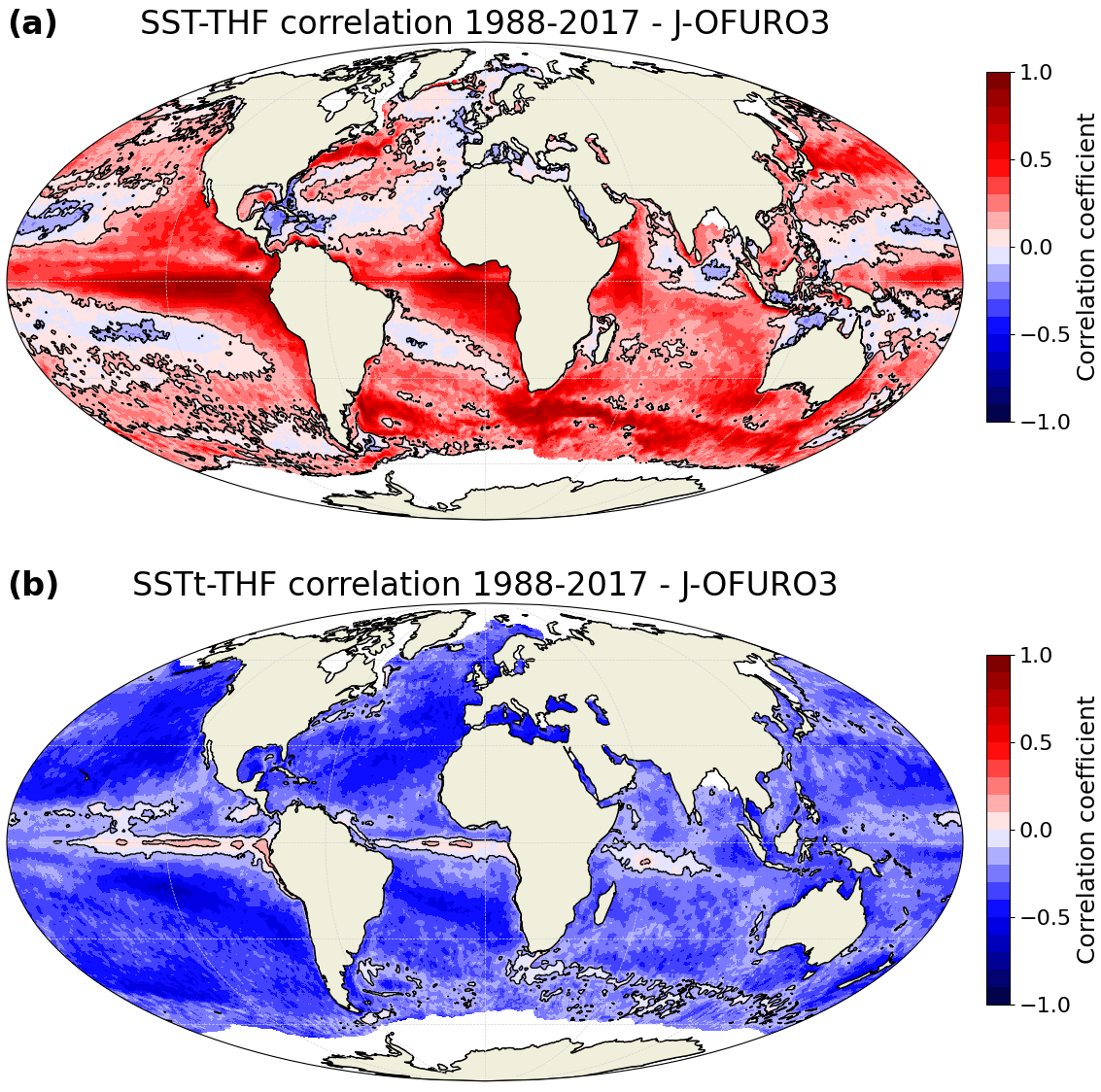
Figure 1 Pearson correlation coefficient (a) between sea surface temperature (SST) and turbulent heat flux (THF) and (b) between SST tendency (SSTt) and THF, based on J-OFURO3 satellite observations. Black contours are drawn around regions with a statistically significant correlation coefficient (FDR 5 %; Student's t test).

Bishop et al. (2017) and Bellucci et al. (2021) showed that regions of high SST gradient and THF (such as the Gulf Stream) are characterized by an ocean-driven regime. In these regions, the SST–THF zero-lag covariance is positive, suggesting that ocean processes drive SST anomalies, and the SST-tendency–THF lead–lag covariance is anti-symmetric (positive covariance at lag −1 and negative covariance at lag +1). On the contrary, an anti-symmetric SST–THF lead–lag covariance and a negative SST-tendency–THF zero-lag covariance are typical of an atmosphere-driven regime (such as in the North Atlantic subtropical gyre). In the latter case, the release of heat flux from the ocean to the atmosphere acts to cool the upper ocean. While this approach is interesting in terms of identifying whether the SST variability is driven by ocean or atmosphere processes, it does not precisely indicate whether the SST causally influences THF or the other way round. In our study, we quantify the causal relationships between SST and/or SST tendency and THF using the rate of information transfer from Liang (2021).

3.1 The two-dimensional (2D) case

If we only take into account SST and THF (i.e., two-dimensional system, hereafter referred to as 2D) in the computation of the rate of information transfer, we find that many regions are characterized by relatively strong two-way influences between SST and THF (Fig. 2). The spatial distribution of the rate of information transfer is relatively similar to the one of the correlation coefficient between SST and THF (Fig. 1a), with the largest values (either positive or negative) in the eastern tropical Pacific and Atlantic regions, western boundary currents and many parts of the Southern Hemisphere. Interestingly, the rate of information transfer is mainly positive for the influence of SST on THF (Fig. 2a), while negative values dominate for the reverse influence (Fig. 2b). This suggests that SST variability generally increases THF variability, while THF variability mainly constrains SST variability. Also, the regions where the influence of SST on THF is strongest are also characterized by a strong influence of THF on SST (in absolute values).

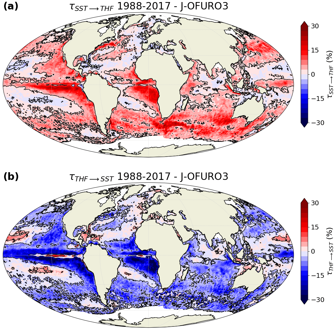
Figure 2 Relative rate of information transfer τ (a) from sea surface temperature (SST) to turbulent heat flux (THF) and (b) from THF to SST, based on J-OFURO3 satellite observations, when two variables are considered. Black contours are drawn around regions with a statistically significant transfer of information (FDR 5 %; 500 bootstrap samples).

Regarding the SST-tendency–THF relationship, using only these two variables in the computation of the rate of information transfer also provides relatively strong two-way influences (either positive or negative) in many regions of the world (Fig. 3). The spatial distribution is more contrasted than with the SST–THF relationship, as both positive and negative values are now present in both directions, especially for the influence of SST tendency on THF (Fig. 3a). The information transfer from SST tendency to THF is characterized by positive southwest–northeast bands in the North Atlantic and North Pacific, positive northwest–southeast bands in the South Atlantic and South Pacific, and negative values between these regions (Fig. 3a). The information transfer from THF to SST tendency shows relatively symmetrical behavior to that from SST tendency to THF, with positive (negative) values where the reverse information transfer is negative (positive; Fig. 3b). This indicates that, in regions where the variability in SST tendency increases (decreases) the variability in THF, the variability in THF decreases (increases) the variability in SST tendency.

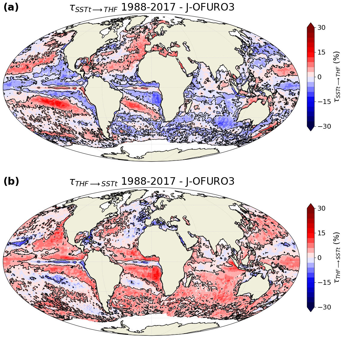
Figure 3 Relative rate of information transfer τ (a) from sea surface temperature tendency (SSTt) to turbulent heat flux (THF) and (b) from THF to SSTt, based on J-OFURO3 satellite observations, when two variables are considered. Black contours are drawn around regions with a statistically significant transfer of information (FDR 5 %; 500 bootstrap samples).

In summary, the 2D analysis shows additional information compared to previous lead–lag correlation studies (Bishop et al., 2017; Bellucci et al., 2021). In particular, we find that the ocean surface influences the lower atmosphere not only in strong boundary currents but also in many other regions of the world (Figs. 2a and 3a). In turn, the lower atmosphere (via surface heat fluxes) influences the ocean surface not only at mid-latitudes but also in tropical regions and western boundary currents (Figs. 2b and 3b). Our results are in line with Bach et al. (2019), who also find significant two-way influences between the upper ocean and lower atmosphere in many regions of the world using the Granger causality but with some methodological differences (daily timescale and other atmospheric fields). This shows that the lead–lag covariance analysis, while interesting in terms of identifying a particular ocean-driven or atmospheric-led regime, is not sufficient to accurately quantify causal links between the upper ocean and lower atmosphere. Importantly, our analysis (like the ones from Bishop et al., 2017 and Bellucci et al., 2021) applies to the monthly timescale, and we will show results beyond this specific timescale in Sect. 3.4.

However, this 2D analysis excludes one of the three key variables considered in the stochastic energy balance model of Wu et al. (2006), either SST tendency in Fig. 2 or SST in Fig. 3. Thus, it may provide a false impression of a two-way influence emerging due to the absence of a hidden variable. Also, the symmetry between the two directions for both the SST–THF (Fig. 2) and SST-tendency–THF (Fig. 3) relationships is questionable due to inaccurate results that were found using a theoretical example (see Sect. 3.5 for further discussion of this aspect). That is why we repeated the computation of the rate of information transfer including all three variables in the next section (Sect. 3.2).

3.2 The three-dimensional (3D) case

We computed the rate of information transfer based on the three variables analyzed in Bishop et al. (2017) and Bellucci et al. (2021), namely SST, SST tendency and THF (hereafter referred to as 3D). The 3D case provides additional sources of information compared to the 2D case and should thus be preferred in terms of result interpretation.

In the 3D case, the influence of SST on THF (Fig. 4a) is very similar to that in the 2D case (Fig. 2a). This is logical, since SST has no significant influence on SST tendency (Fig. B2), so all the information from SST goes to THF, demonstrating the robustness of the approach. However, a much-reduced number of regions shows a significant rate of information transfer from THF to SST (Fig. 4b) compared to that in the 2D case (Fig. 2b). This reduction is due to the fact that we now take SST tendency into account in the computation of the rate of information transfer; part of the information transfer from THF also goes into SST tendency, as we will see below. Despite this reduction in the number of regions with a significant transfer of information, the eastern tropical Pacific and Atlantic regions still show a strong negative rate of information transfer, suggesting that THF variability constrains SST variability in these regions (Fig. 4b). Interestingly, some regions (such as the Agulhas Return Current) show a positive rate of information transfer from THF to SST in the 3D case (Fig. 4b), while it is negative or close to 0 in the 2D case (Fig. 2b).

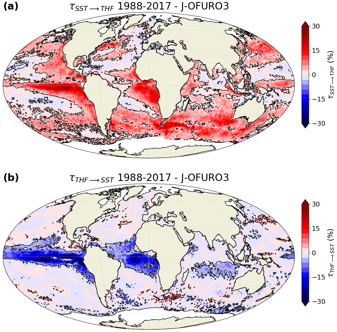
Figure 4 Relative rate of information transfer τ (a) from sea surface temperature (SST) to turbulent heat flux (THF) and (b) from THF to SST, based on J-OFURO3 satellite observations, when three variables are considered (SST, SST tendency and THF). Black contours are drawn around regions with a statistically significant transfer of information (FDR 5 %; 500 bootstrap samples).

In the 3D case, the rate of information transfer from SST tendency to THF (Fig. 5a) is very similar to that in the 2D case (Fig. 3a) for the same reason as for the SST–THF influence. However, a much-reduced number of regions shows a significant transfer of information from THF to SST tendency (Fig. 5b) compared to that in the 2D case (Fig. 3b). Similarly as for the influence of THF on SST, this is due to the inclusion of a third variable; specifically, part of the information transfer from THF also goes into SST. Nevertheless, we still find regions of significant influence, e.g., negative values in the North Atlantic and northeastern Pacific and positive values in tropical regions.

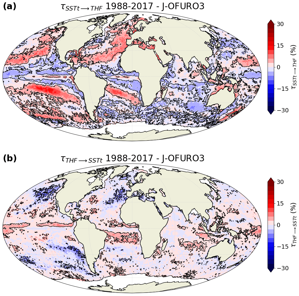
Figure 5 Relative rate of information transfer τ (a) from sea surface temperature tendency (SSTt) to turbulent heat flux (THF) and (b) from THF to SSTt, based on J-OFURO3 satellite observations, when three variables are considered (SST, SST tendency and THF). Black contours are drawn around regions with a statistically significant transfer of information (FDR 5 %; 500 bootstrap samples).

Thus, computing the rate of information transfer based on the three variables of interest (SST, SST tendency and THF) somehow partitions the total influence of the lower atmosphere (THF) into a contribution to SST (Fig. 4b) and another contribution to SST tendency (Fig. 5b). Additionally, the total number of regions with a significant influence by THF on SST and by THF on SST tendency (both combined) clearly decreases compared to the 2D case. As the influences of SST on THF and of SST tendency on THF remain strong in the 3D case (almost unchanged compared to the 2D case), this is in favor of a stronger ocean influence compared to the atmosphere influence at monthly timescale, especially in extra-tropical regions.

In western boundary currents, we find large values of the rate of information transfer from SST to THF (Fig. 4a), suggesting a strong ocean influence, in agreement with Bishop et al. (2017). However, in extra-tropical regions far away from western boundary currents, such as in the central North Atlantic, we also find a strong transfer of information from SST (Fig. 4a) and from SST tendency (Fig. 5a) to THF, which is generally stronger than the reverse influence (from THF to SST and to SST tendency). This somewhat brings into question previous findings that suggest an atmospheric-driven SST variability in these regions (Bishop et al., 2017; Bellucci et al., 2021), and this shows that lead–lag covariance analyses should be supplemented by causality studies. The use of the SeaFlux observational dataset provides results that are in broad agreement with J-OFURO3 (Figs. B3–B4), which confirms the robustness of our findings.

The extension to additional variables can of course be performed to refine the analysis further, making sure that the additional variables are not nearly parallel (otherwise, the singularity of the covariance matrix could numerically deteriorate the results). We can do this by including other fields, higher-order tendencies or lagged fields. A first step toward an analysis of such a type is provided below. In our study, we prefer to keep the three fields used in the stochastic energy balance model from Wu et al. (2006) and analyzed by Bishop et al. (2017) and Bellucci et al. (2021), i.e., SST, SST tendency and THF. We will therefore focus on the use of a lagged field (Sect. 3.3), as well as on the analysis of interannual to decadal variability (Sect. 3.4).

3.3 Lagged transfer of information

Due to the inertia of the ocean mixed layer, the SST does not necessarily respond directly to changes in THF (Deser et al., 2003; Shi et al., 2022). To take this effect into account, we added a fourth variable to our analysis, namely THF leading SST by 1 month, hereafter referred to as THF(-1). Thus, the following four variables are considered here: SST, SST tendency, THF and THF(-1). The rate of information transfer has been applied to lagged variables in a previous study to predict El Niño Modoki based on solar activity (Liang et al., 2021). Note that the rate of information is not entirely free of time lag, as it involves a tendency term (d$X_i/$dt in Eq. 1), which is estimated in a discrete way.

We find that there is a significant positive rate of information transfer from THF(-1) to SST in eastern tropical Pacific and Atlantic regions, western boundary currents (Gulf Stream and Kuroshio Extension) and the Agulhas Return Current, as well as negative values in other parts of the world (Fig. 6a). Thus, the lagged analysis shows that THF taken 1 month before strongly controls SST variability, especially in northern extra-tropical regions where this influence is almost absent in the original 3D case (Fig. 4b). There is also additional information provided by this fourth variable in the transfer of information from THF(-1) to SST tendency (Fig. 6b), but this is mostly restricted to the eastern tropical Pacific and Atlantic (negative values). The influence of SST and/or SST tendency on THF(-1) is found to be very close to 0 and to be not significant almost everywhere (Fig. B5), which confirms the robustness of the method, as causality cannot go back in time.

Interestingly, most regions showing a positive rate of information transfer from THF(-1) to SST (Fig. 6a) also have a positive lead–lag covariance between THF(-1) and SST (Fig. 3c of Bishop et al., 2017). Bishop et al. (2017) show that these regions have a symmetric lead–lag structure between SST and THF, which is characteristic of an ocean-driven regime. However, these similarities between the rate of information transfer and the lead–lag covariance disappear when we look at the relationships between THF(-1) and SST tendency. According to Bishop et al. (2017), the strongest values of lead–lag covariance between THF(-1) and SST tendency appear in western boundary currents (negative values; Fig. 3f of Bishop et al., 2017), while the rate of information transfer is significant only in the eastern tropical Pacific and Atlantic (negative values; Fig. 6b).

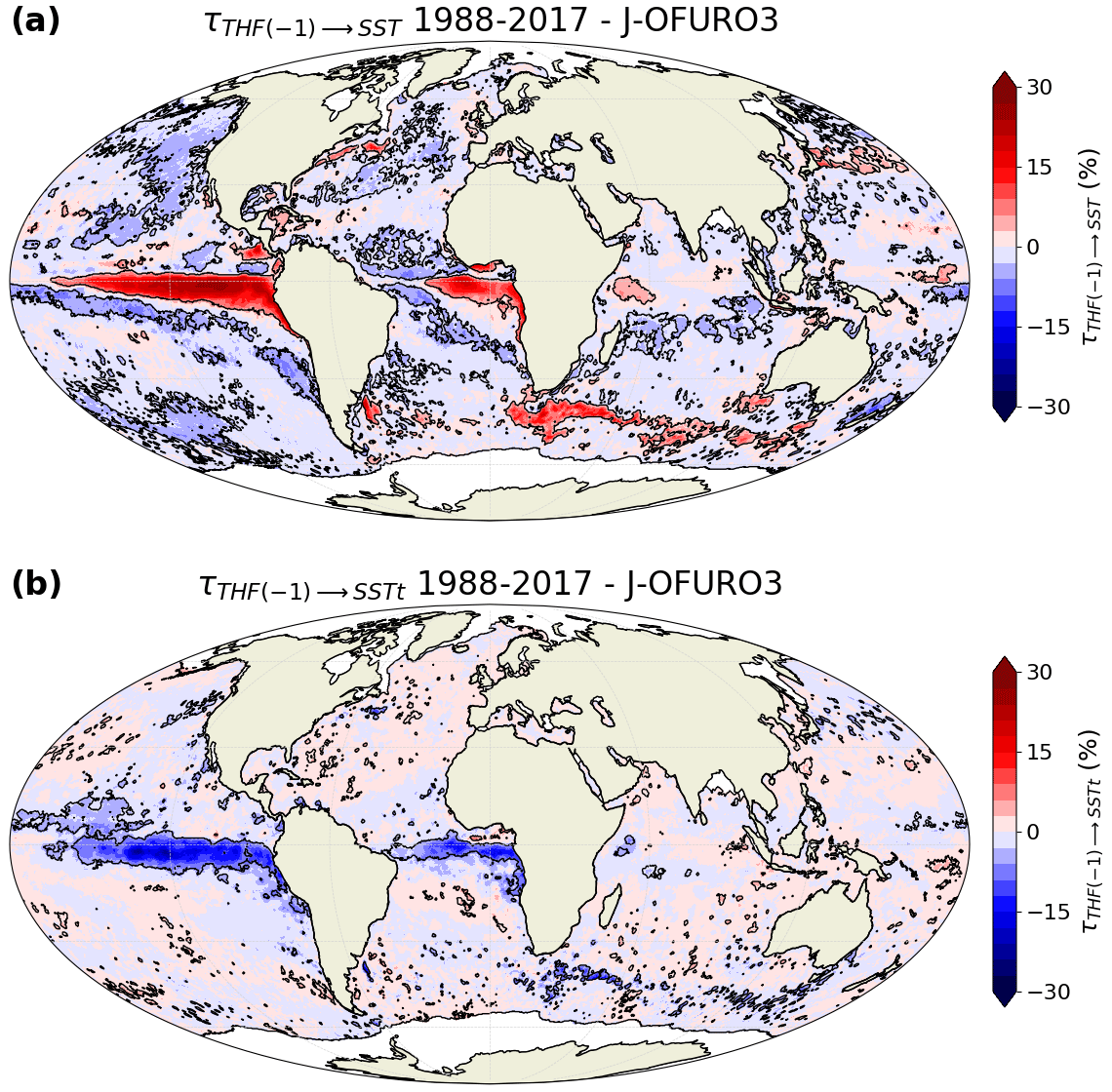
Figure 6 Relative rate of information transfer τ (a) from turbulent heat flux at lag −1 (THF(-1) – THF leading SST by 1 month) to sea surface temperature (SST) and (b) from THF(-1) to SST tendency (SSTt), based on J-OFURO3 satellite observations, when four variables are considered (SST, SST tendency, THF and THF(-1)). Black contours are drawn around regions with a statistically significant transfer of information (FDR 5 %; 500 bootstrap samples).

3.4 Interannual to decadal variability

All previous results are based on monthly mean outputs. Thus, our results are valid at a monthly timescale. In order to figure out what happens at interannual and decadal timescales, we take the 12- and 120-month (respectively) running-mean SST and THF (moving average with the same number of samples), and we re-compute the rate of information transfer in the 3D case (SST, SST tendency and THF). This approach is similar to the one used in Vannitsem and Liang (2022), who found differences in the rate of information transfer between climate indices depending on the timescale used.

At the interannual timescale (12-month running mean), the influence of SST on THF encompasses approximately the same regions as at a monthly timescale but with a general increase in the magnitude of the rate of information transfer (Fig. 7a). We also find regions that have a negative rate of information transfer, such as in the western North Atlantic Ocean, whereas such regions are not present with monthly means. The reverse influence of THF on SST provides a more contrasted pattern compared to that in the original 3D case, with a reduced number of regions with negative values along the Equator but also the additional presence of regions with positive values (Fig. 7b).

Figure 7 Relative rate of information transfer τ (a) from sea surface temperature (SST) to turbulent heat flux (THF) and (b) from THF to SST, based on J-OFURO3 satellite observations, when three variables are considered (SST, SST tendency and THF) and using a 12-month running mean (interannual variability). Black contours are drawn around regions with a statistically significant transfer of information (FDR 5 %; 500 bootstrap samples).

At a decadal timescale (120-month running mean), almost the whole globe is covered by significant information transfer between SST and THF in the two directions (Fig. 8). Also, the magnitude of the rate of information transfer clearly increases at this timescale compared to at interannual and decadal timescales. These results suggest that ocean-atmosphere interactions become more pronounced at larger timescales.

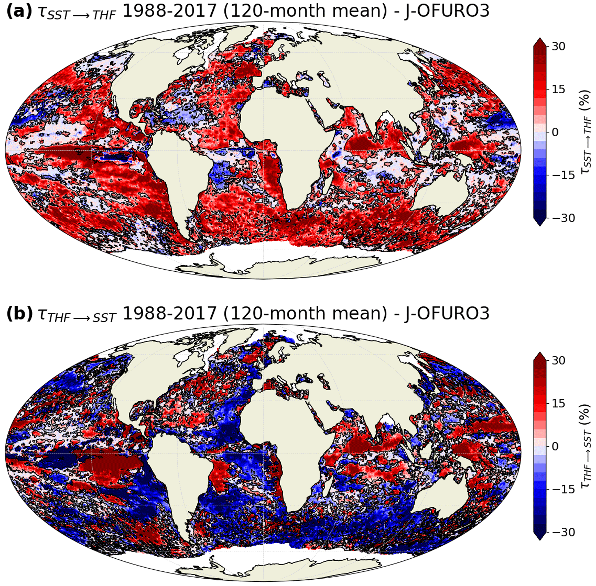
Figure 8 Relative rate of information transfer τ (a) from sea surface temperature (SST) to turbulent heat flux (THF) and (b) from THF to SST, based on J-OFURO3 satellite observations, when three variables are considered (SST, SST tendency and THF) and using a 120-month running mean (decadal variability). Black contours are drawn around regions with a statistically significant transfer of information (FDR 5 %; 500 bootstrap samples).

3.5 Limitations of the method

The rate of information transfer used in our study has major advantages compared to other causal methods, including its derivation from the first principles of information entropy (Liang, 2016) and its relative simplicity (Eq. 1). However, several limitations exist, which need to be kept in mind.

The first limitation arises from the linearity assumption (Liang, 2014). While the method has been tested and validated with highly nonlinear synthetic examples (e.g., Liang, 2014, 2018, 2021), it provides an approximated solution, and a generalization to the fully nonlinear case is still to be developed to get a more accurate solution (Liang, 2021). However, recent studies applying the rate of information transfer to climate data show that the method is successful at representing some key causal influences, such as the interactions between El Niño and the Indian Ocean Dipole (Liang, 2014), CO₂ and global mean temperature (Stips et al., 2016), and Arctic sea ice and its drivers (Docquier et al., 2022).

The second limitation is linked to the problem of hidden variables. If we omit an important variable in our system, the rates of information transfer might be biased. In our specific study, some differences appear between the 2D case and the 3D case (Sect. 3.2). As we do not include one of the key variables of the stochastic energy balance model designed by Wu et al. (2006) in the 2D case, we end up with a biased result. In particular, the rate of information transfer from THF to SST is overestimated in northern and southern extratropical regions (compare Fig. 2b to Fig. 4b). This overestimation also appears in the rate of information transfer from THF to SST tendency (compare Fig. 3b to Fig. 5b). Also, a relatively symmetric behavior appears in the 2D case between both causal directions for the SST–THF relationship (Fig. 2) and for the SST-tendency–THF relationship (Fig. 3), although a number of regions do not show such a symmetry. This somehow goes in hand with the inaccurate symmetry obtained in computing the rate of information transfer in the unidirectionally coupled Rössler systems (Paluš et al., 2018) when using only two variables (Paluš, 2022; Fig. C1f). Thus, the results obtained in the 2D case in our study must be taken with great care, and 3D results should be privileged. Further research should be carried out to better understand the impact of hidden variables in computing the rate of information transfer.

Finally, the information flow method depends on the sampling frequency when applied to unidirectionally coupled Rössler systems and possibly to other systems and real-case studies. In the case of the Rössler systems, the method becomes inaccurate when the sampling frequency is too coarse (Appendix C; Fig. C1a–e). In our real-case study, it is difficult to accurately quantify this effect due to the shortness of the time period (360 months). Further research is needed to better understand the effect of the sampling frequency on the computation of the rate of information transfer.

4 Conclusions

In summary, we find that the rate of information transfer provides a more detailed quantification of dependencies between SST, SST tendency and turbulent heat flux (THF) than previous classical correlation–covariance studies. We do not argue that causal methods should replace covariance analyses, but they should rather be used as a complement in order to get a better understanding of physical interactions between variables. We show that the ocean surface (SST and SST tendency) strongly drives changes in the lower atmosphere (THF) and that the lower atmosphere also has an important influence on the ocean surface in many regions of the world. This result is somewhat different from what has been found in covariance analyses, in which ocean-driven regimes exist in western boundary currents and where atmospheric-led regimes dominate in the open ocean (Bishop et al., 2017; Bellucci et al., 2021). It is, however, supported by another recent analysis using the Granger causality, which shows that many regions of the world present a significant two-way influence between the lower atmosphere and the upper ocean, with a stronger ocean influence in tropical regions and a stronger atmospheric impact in the extra-tropics (Bach et al., 2019). As the latter study presents methodological differences – i.e., it focuses on the daily timescale and uses different atmospheric variables – we need to be cautious in comparing it to our analysis. In any case, our interpretation of these results is that ocean–atmosphere interactions are more complex than presented by classical covariance analyses.

Furthermore, we find that the influence of THF is partitioned between SST and SST tendency if we consider the three variables together (3D case, which should be privileged due to the inclusion of additional sources of information) so that the single impact of either THF on SST or of THF on SST tendency is decreased in the 3D case compared to that in the 2D case. Also, the number of regions with a significant rate of information transfer from THF to SST and from THF to SST tendency (combined) is smaller than the one with a significant rate of information transfer from SST to THF and from SST tendency to THF (combined) in the 3D case. This suggests an overall stronger upper-ocean influence compared to the lower atmosphere. However, when adding THF taken 1 month before to take the lagged effect into account, we find that this variable has a relatively strong influence on SST in a large portion of the globe. Finally, a larger timescale (going from monthly to interannual and decadal) provides larger values in terms of the rates of information transfer between the three variables.

In our study, we only considered the ocean surface, but several studies have shown that variations in the ocean heat content are controlled by both air–sea fluxes and ocean heat transport convergence, with a more important role for the latter with a deeper integration of ocean heat and with higher-resolution climate models (Roberts et al., 2017; Small et al., 2020). Also, only observations were considered here. Thus, extending our analysis to the ocean heat budget terms in climate models would provide further insights into the causal influences between the ocean and atmosphere. This is of large importance, as ocean–atmosphere interactions constitute an important regulator of our climate. Finally, from a theoretical perspective, additional investigations of the role of hidden and lagged variables should be performed, as well as a comparison of the rate of information transfer to other causal methods.

Appendix A: Impact of the rate of information transfer on the variability

As explained in the main text (Sect. 2.2), a positive value of the relative rate of information transfer τ_j→i means that the variability in X_j increases the variability in X_i, while a negative value means that the variability in X_j decreases the variability in X_i. More broadly, an increase in the rate of information transfer from X_j to X_i leads to an increase in the variability of X_i. We demonstrate this by computing the rate of information transfer τ_j→i from variable X_j to variable X_i (based on Eq. 3 in the main text) using a three-dimensional stochastic linear system of equations as follows:

$$\begin{array}{}\text{(A1)}& \begin{array}{rlrl}& \mathrm{d}{X}_{\mathrm{1}}& =& (a_{\mathrm{11}}{X}_{\mathrm{1}}+a_{\mathrm{12}}{X}_{\mathrm{2}}+a_{\mathrm{13}}{X}_{\mathrm{3}})\mathrm{d}t+\mathrm{0.1}\mathrm{d}{W}_{\mathrm{1}},\\ & \mathrm{d}{X}_{\mathrm{2}}& =& (a_{\mathrm{21}}{X}_{\mathrm{1}}+a_{\mathrm{22}}{X}_{\mathrm{2}}+a_{\mathrm{23}}{X}_{\mathrm{3}})\mathrm{d}t+\mathrm{0.1}\mathrm{d}{W}_{\mathrm{2}},\\ & \mathrm{d}{X}_{\mathrm{3}}& =& (a_{\mathrm{31}}{X}_{\mathrm{1}}+a_{\mathrm{32}}{X}_{\mathrm{2}}+a_{\mathrm{33}}{X}_{\mathrm{3}})\mathrm{d}t+\mathrm{0.1}\mathrm{d}{W}_{\mathrm{3}},\end{array}\end{array}$$

where X₁, X₂ and X₃ are the three variables; a_kl are the different coefficients; t is time and varies between 0 and 100 with 100 000 time steps (Δt=0.001); and W₁, W₂ and W₃ represent normal random noises (standard Wiener process). We set $a_{\mathrm{11}}=a_{\mathrm{22}}=a_{\mathrm{33}}=-\mathrm{1}$, and we vary the six other coefficients one by one with five different values between −1 and 1 (−1, −0.5, 0, 0.5 and 1). When varying one of the six coefficients, we set the other five coefficients to a fixed value ($a_{\mathrm{12}}=a_{\mathrm{13}}=\mathrm{0.5}$ and $a_{\mathrm{21}}=a_{\mathrm{23}}=a_{\mathrm{31}}=a_{\mathrm{32}}=\mathrm{0}$).

We solve the linear system (A1) using the Euler–Maruyama method, and 40 different values of the random noise are taken in order to take into account the uncertainty related to the rate of information transfer. The variance in each variable is compared to the rate of information transfer from any other variable to this variable to test our hypothesis. Results show that when the rate of information transfer from X_j to X_i increases, the variance in X_i increases (Fig. A1).

Figure A1 Variance σ² of a variable as a function of the relative rate of information transfer τ from any other variable to this variable using the linear system of Eq. (A1). The error bars show the 95 % confidence intervals of the rates of information transfer.

Appendix B: Additional figures

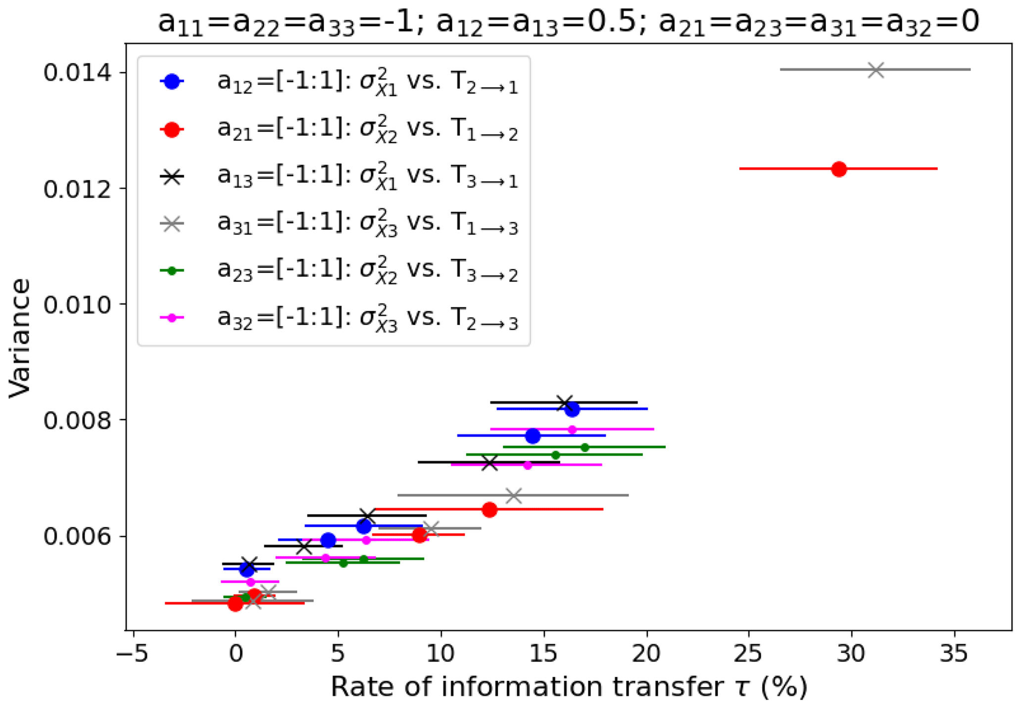
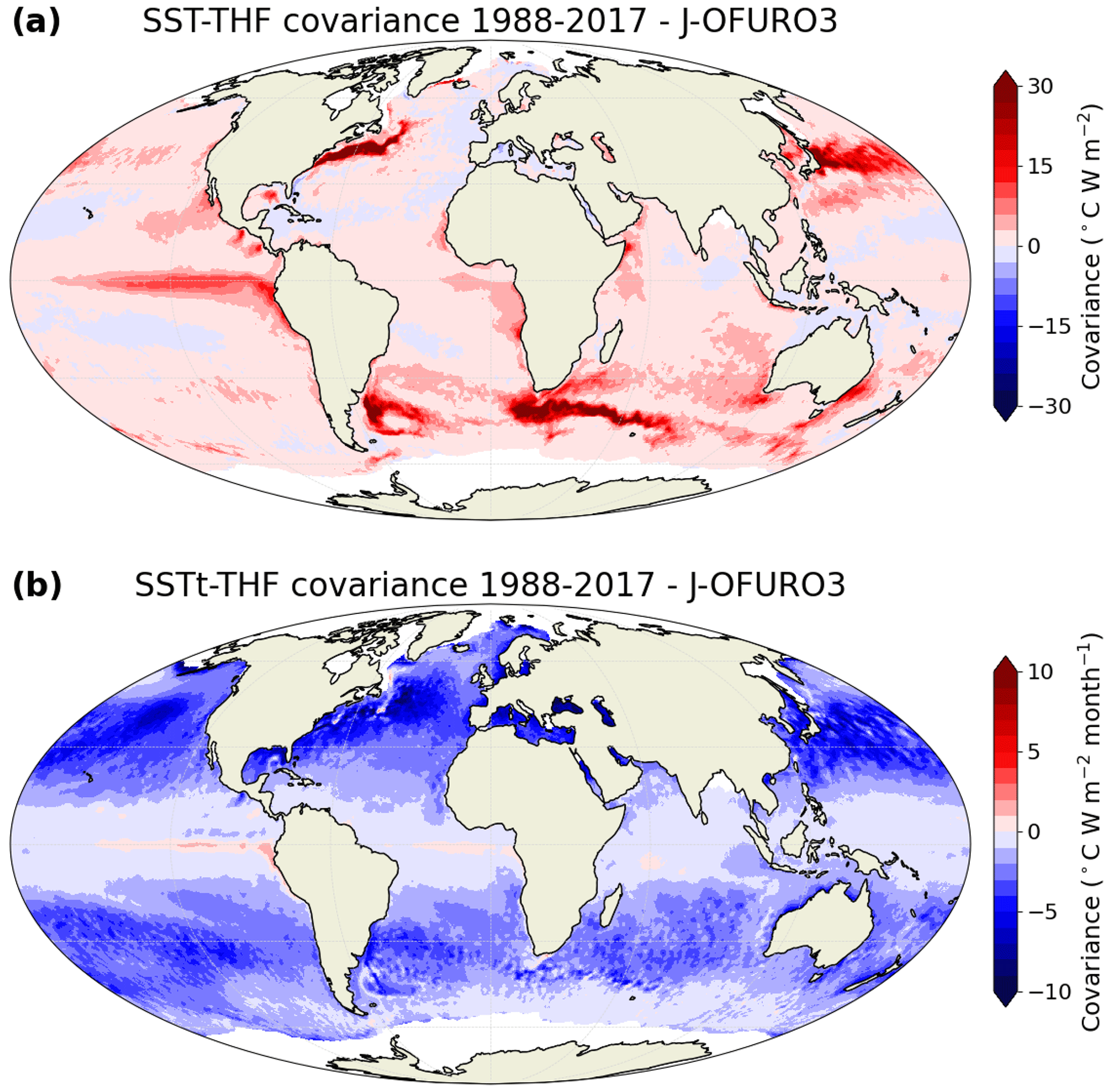
Figure B1 Covariance (a) between sea surface temperature (SST) and turbulent heat flux (THF) and (b) between SST tendency (SSTt) and THF, based on J-OFURO3 satellite observations.

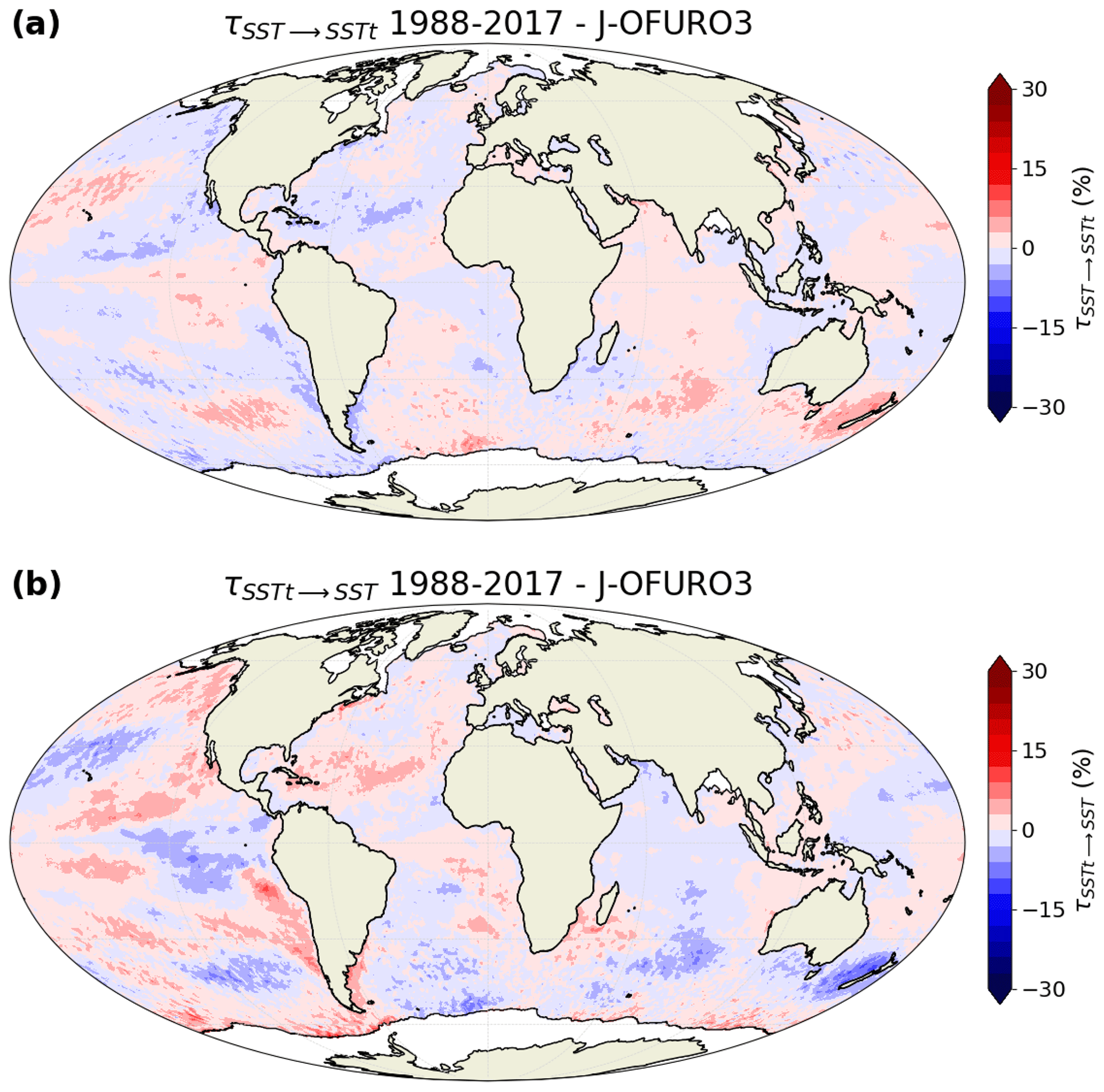
Figure B2 Relative rate of information transfer τ (a) from sea surface temperature (SST) to SST tendency and (b) from SST tendency to SST, based on J-OFURO3 satellite observations, when three variables are considered (SST, SST tendency and THF). None of the grid points shows a statistically significant transfer of information (FDR 5 %; 500 bootstrap samples).

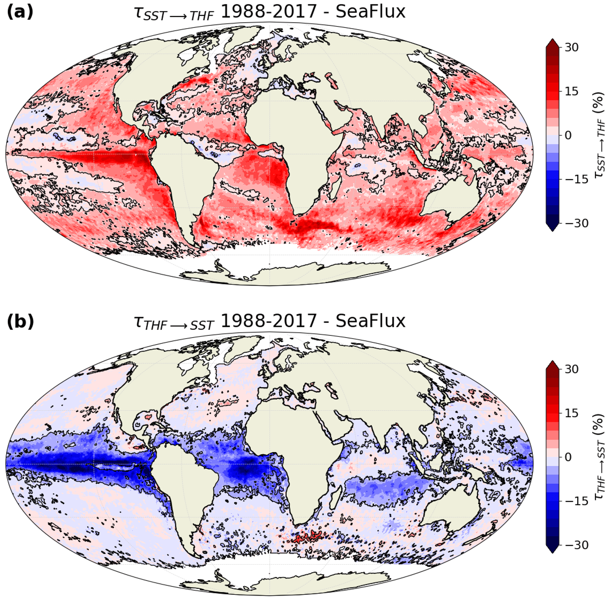
Figure B3 Relative rate of information transfer τ (a) from sea surface temperature (SST) to turbulent heat flux (THF) and (b) from THF to SST, based on SeaFlux satellite observations, when three variables are considered (SST, SST tendency and THF). Black contours are drawn around regions with a statistically significant transfer of information (FDR 5 %; 500 bootstrap samples).

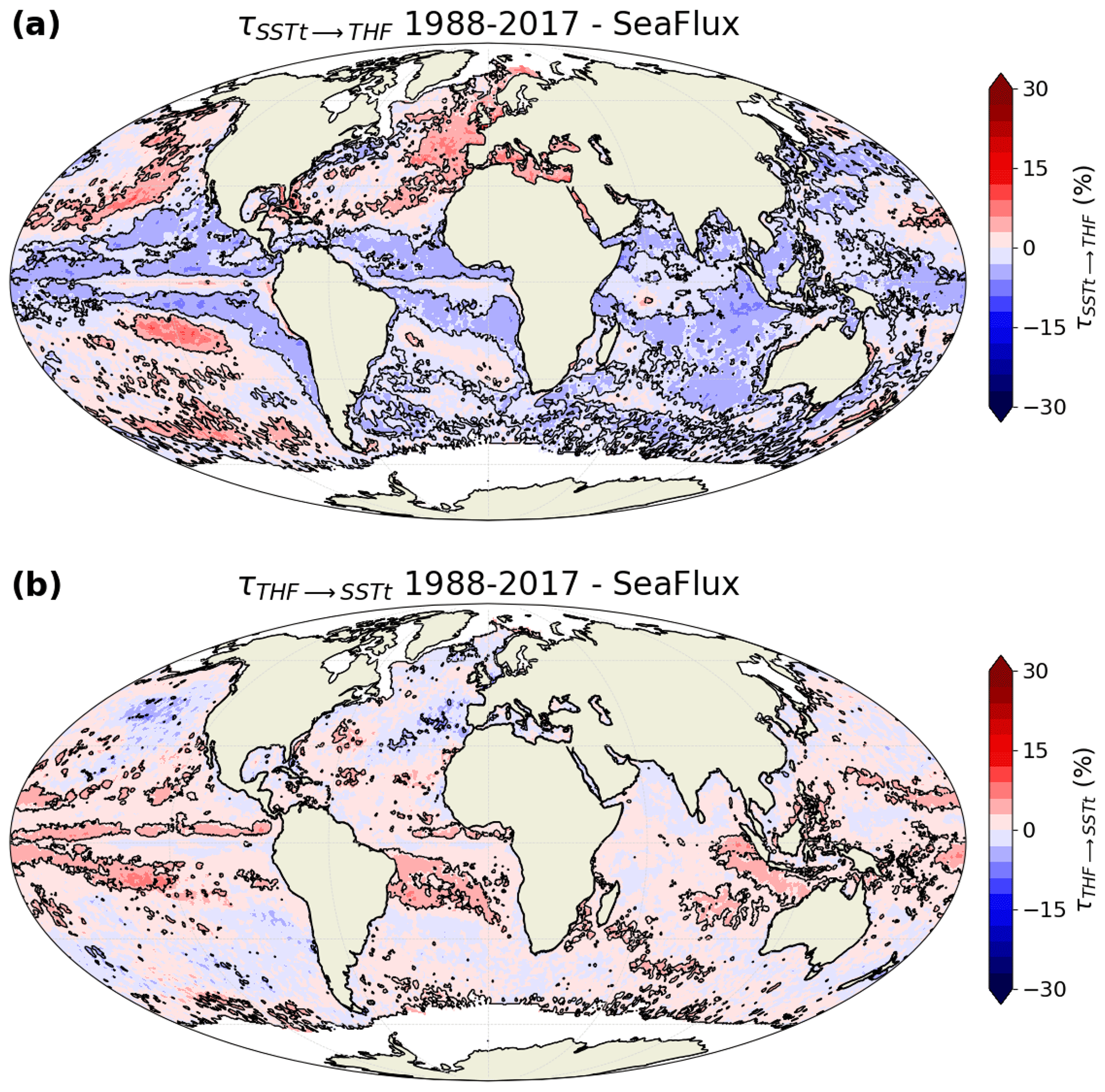
Figure B4 Relative rate of information transfer τ (a) from sea surface temperature tendency (SSTt) to turbulent heat flux (THF) and (b) from THF to SSTt, based on SeaFlux satellite observations, when three variables are considered (SST, SST tendency and THF). Black contours are drawn around regions with a statistically significant transfer of information (FDR 5 %; 500 bootstrap samples).

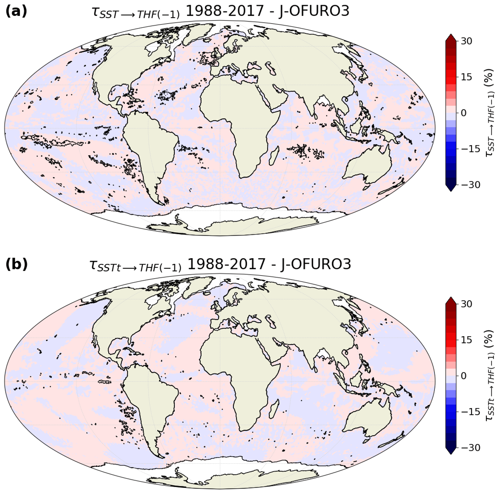
Figure B5 Relative rate of information transfer τ (a) from sea surface temperature (SST) to turbulent heat flux 1 month before (THF(-1)) and (b) from SST tendency to THF(-1), based on J-OFURO3 satellite observations, when four variables are considered (SST, SST tendency, THF and THF(-1)). Black contours are drawn around regions with a statistically significant transfer of information (FDR 5 %; 500 bootstrap samples).

Appendix C: Dependence on the sampling frequency

In order to test the dependence of the information flow method on the sampling frequency, we compute the absolute rate of information transfer (Eq. 1) on the two unidirectionally coupled Rössler systems using the same parameters as Paluš and Vejmelka (2007) and Paluš et al. (2018) as follows:

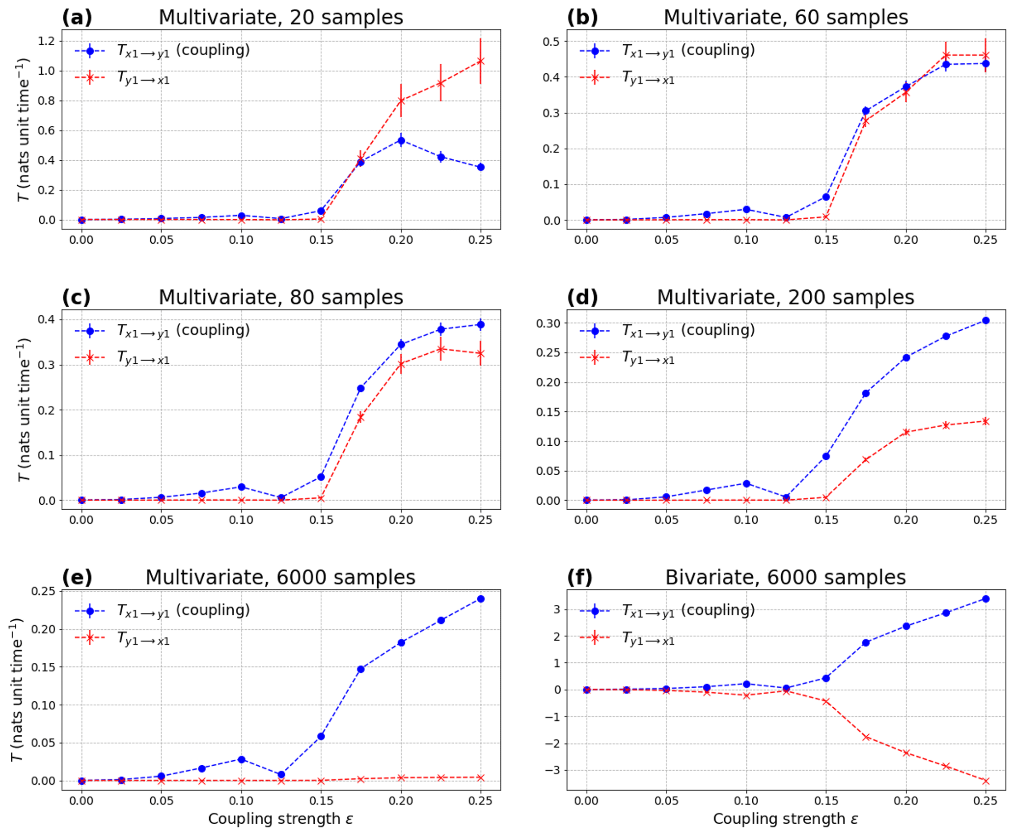
Figure C1 Absolute rate of information transfer T (multivariate formula) as a function of the coupling strength ϵ applied to unidirectionally coupled Rössler systems with (a) 20, (b) 60, (c) 80, (d) 200 and (e) 6000 samples per pseudo-period; (f) is similar to (e), except that the bivariate formula is used instead. The sign of T is kept in all panels.

$$\begin{array}{}\text{(C1)}& \begin{array}{rl}& \mathrm{d}{x}_{\mathrm{1}}/\mathrm{d}t=-{\mathit{\omega }}_{\mathrm{1}}{x}_{\mathrm{2}}-x_{\mathrm{3}},\\ & \mathrm{d}{x}_{\mathrm{2}}/\mathrm{d}t={\mathit{\omega }}_{\mathrm{1}}{x}_{\mathrm{1}}+a_{\mathrm{1}}{x}_{\mathrm{2}},\\ & \mathrm{d}{x}_{\mathrm{3}}/\mathrm{d}t=b_{\mathrm{1}}+x_{\mathrm{3}}(x_{\mathrm{1}}-c_{\mathrm{1}}),\\ & \mathrm{d}{y}_{\mathrm{1}}/\mathrm{d}t=-{\mathit{\omega }}_{\mathrm{2}}{y}_{\mathrm{2}}-y_{\mathrm{3}}+\mathit{ϵ}(x_{\mathrm{1}}-y_{\mathrm{1}}),\\ & \mathrm{d}{y}_{\mathrm{2}}/\mathrm{d}t={\mathit{\omega }}_{\mathrm{2}}{y}_{\mathrm{1}}+a_{\mathrm{2}}{y}_{\mathrm{2}},\\ & \mathrm{d}{y}_{\mathrm{3}}/\mathrm{d}t=b_{\mathrm{2}}+y_{\mathrm{3}}(y_{\mathrm{1}}-c_{\mathrm{2}}),\end{array}\end{array}$$

where ω₁=1.015, ω₂=0.985, $a_{\mathrm{1}}=a_{\mathrm{2}}=\mathrm{0.15}$, $b_{\mathrm{1}}=b_{\mathrm{2}}=\mathrm{0.2}$ and $c_{\mathrm{1}}=c_{\mathrm{2}}=\mathrm{10}$. We use the same time step for integration as Paluš et al. (2018); i.e., dt=0.0785. We use the same initialization method as Paluš et al. (2018), solve the equations using the fourth-order Runge–Kutta scheme, and run the model for 7.5 × 10⁶ time steps. We discard the first 1.5 × 10⁶ time steps from the analysis. We use a coupling strength ϵ that varies between 0 and 0.25 with an increment of 0.025. We test different numbers of samples per pseudo-period and retain here the five of them (20, 60, 80, 200 and 6000) that best illustrate our results.

As illustrated in Fig. C1, results depend on the number of samples per pseudo-period. When using 20 samples per pseudo-period, $T_{y\mathrm{1}\to x\mathrm{1}}>T_{x\mathrm{1}\to y\mathrm{1}}$ when the coupling strength ϵ≥0.2, which is physically not correct (Fig. C1a). For 60 samples per pseudo-period, both influences are comparable for larger coupling strengths (Fig. C1b). From 80 samples per pseudo-period, $T_{x\mathrm{1}\to y\mathrm{1}}>T_{y\mathrm{1}\to x\mathrm{1}}$ (Fig. C1c–e), which is physically correct, and one needs to reach ∼ 6000 samples per pseudo-period to have $T_{y\mathrm{1}\to x\mathrm{1}}=\mathrm{0}$ (Fig. C1e). Importantly, all six variables need to be considered in the computation of the rate of information transfer (multivariate formula; Liang, 2021) to reach this result. If we only consider X₁ and Y₁ and compute the rate of information transfer using the bivariate formula (Liang, 2014), we obtain an inaccurate result with a symmetry between the two directions whatever the number of samples per pseudo-period (Fig. C1f).