the Creative Commons Attribution 4.0 License.
the Creative Commons Attribution 4.0 License.
 | 26 Apr 2023
Direct and indirect application of univariate and multivariate bias corrections on heat-stress indices based on multiple regional-climate-model simulations
Seung-Ki Min
Yeon-Hee Kim
Dong-Hyun Cha
Seok-Woo Shin
Joong-Bae Ahn
Eun-Chul Chang
Young-Hwa Byun
Statistical bias correction (BC) is a widely used tool to post-process climate model biases in heat-stress impact studies, which are often based on the indices calculated from multiple dependent variables. This study compares four BC methods (three univariate and one multivariate) with two correction strategies (direct and indirect) for adjusting two heat-stress indices with different dependencies on temperature and relative humidity using multiple regional climate model simulations over South Korea. It would be helpful for reducing the ambiguity involved in the practical application of BC for climate modeling and end-user communities. Our results demonstrate that the multivariate approach can improve the corrected inter-variable dependence, which benefits the indirect correction of heat-stress indices depending on the adjustment of individual components, especially those indices relying equally on multiple drivers. On the other hand, the direct correction of multivariate indices using the quantile delta mapping univariate approach can also produce a comparable performance in the corrected heat-stress indices. However, our results also indicate that attention should be paid to the non-stationarity of bias brought by climate sensitivity in the modeled data, which may affect the bias-corrected results unsystematically. Careful interpretation of the correction process is required for an accurate heat-stress impact assessment.
- Article
(6873 KB) - Full-text XML
-
Supplement
(986 KB) - BibTeX
- EndNote


Climate models unavoidably produce biased representations of the simulated variables, and it is more problematic not to know how these biases translate into the modeled response to external forcings such as the CO2 concentration, which is known to be responsible for global warming. Therefore, statistical bias correction (BC) of climate model outputs has been progressively adopted as a standard procedure to improve their performance, in particular when feeding them into various climate change impact assessments (e.g., G. Kim et al., 2020; Kim et al., 2022; Masaki et al., 2015; Qiu et al., 2022; Schwingshackl et al., 2021). Indeed, the visible benefits archived by adjusting simple statistics (e.g., mean, variance) have led to the wide application of BC. A significant body of research demonstrated that the systematic biases observed in the long-term pattern of the current climate can be well eliminated even when using a very simple technique (e.g., linear scaling). However, the effectiveness of BC methods and their improper assumptions (e.g., statistical stationarity) remain a topic for debate (Maraun et al., 2017). For example, the non-stationary model bias and the large monthly/seasonal correction factor can potentially degrade the BC's performance, particularly with respect to misleading interpretations of extremes (Chen et al., 2021; Lee et al., 2019). Meanwhile, the choice of BC approaches in different contexts (e.g., heat-stress impact study, hydrological impact study, adjustment of boundary conditions in downscaling) needs careful assessment on a case-by-case basis (Ehret et al., 2012; Rocheta et al., 2017; Kim et al., 2022; Zscheischler et al., 2019).
A variety of BC methods with different levels of complexity and performance have been developed and implemented for both global and regional climate simulations (François et al., 2020; Teutschbein and Seibert, 2012; Kim et al., 2021). Generally, their aim is to correct certain features in the target's distribution, such as the simple statistics of the mean (linear scaling, LS; Teutschbein and Seibert, 2012) and variance (variance scaling, VA; Chen and Dudhia, 2001) or the more advanced quantiles (quantile mapping, QM) for adjusting the entire distribution by parametric (PQM) or empirical (EQM) transformation (Switanek et al., 2017; Gudmundsson et al., 2012). Continuous efforts have also been made to eliminate the drawbacks of existing BC approaches. Quantile delta mapping (QDM; Cannon et al., 2015), for example, is designed to explicitly preserve the long-term trend that may be artificially distorted in QM. Nonetheless, all the approaches described above correct bias in a univariate context. They cannot adjust the inter-variable dependencies, which are important for representing physical processes and estimating compound hazards. It was not until quite recently that the multivariate BC technique was considered and proposed (e.g., Bárdossy and Pegram, 2012; Cannon, 2018; Mehrotra and Sharma, 2015, 2016; Robin et al., 2019; Vrac, 2018), and they have been applied to various climate change impact studies (Zscheischler et al., 2019; Qiu et al., 2022; Meyer et al., 2019; Dieng et al., 2022). Although it is intuitively recognized that multivariate BC could be more suitable for dealing with climate variables characterized by a strong physical linkage in nature, an unambiguous assessment of univariate and multivariate BC methods is essential to understand the potential limitations of individual methods and to avoid misleading application.
Despite the BC method used, when correcting the multivariate indices representing compound hazards, the index can also be either directly adjusted using BC techniques, as in the majority of studies (Schwingshackl et al., 2021; Kang et al., 2019; Coffel et al., 2017), or indirectly corrected so that its components are individually corrected prior to the index calculation (Casanueva et al., 2019; Zscheischler et al., 2019). In this regard, there have been few systematic comparisons of how the direct and indirect use of univariate and multivariate BC methods, respectively, affect the multivariate indices' adjustment. Only Casanueva et al. (2018) tested the direct and indirect use of EQM in correcting the multivariate fire danger index, while several studies compared the indirect use of univariate and multivariate BC methods in impact assessments (e.g., Cannon, 2018; François et al., 2020; Zscheischler et al., 2019). Although Casanueva et al. (2018) pointed out that the direct application of EQM outperforms the indirect one, how it compares with the multivariate BC method remains unknown. Therefore, there is room for a more comprehensive assessment of the effects of univariate and multivariate BC under direct and indirect application strategies, which may vary along with the dependence structure of the multivariate indices and may affect correction efficiency since the multivariate approach has a higher computation cost.
In this study, we investigate the effects of different BC methods (univariate vs. multivariate) applied with different strategies (direct vs. indirect) on the statistical adjustment of heat-stress indices that represent the combined effect of human exposure to temperature (T) and relative humidity (RH), using regionally tailored, fine-scale climate information in Korea from multiple regional climate models (RCMs). The extreme heat is one of the most critical impacts of climate change, and we adopt two heat-stress indices with different sensitivities to humidity (Sherwood, 2018), namely wet-bulb globe temperature (WBGT) and apparent temperature (AT). A comparative assessment of the two indices derived from different BC methods and different strategies will provide valuable insights into understanding how the relationship between heat-stress index and its drivers (e.g., T and RH) affects the performance of univariate and multivariate BC for modeled heat stress. This study will be helpful for reducing the ambiguity involved in the practical application of BC for climate modeling as well as end-user communities.
2.1 Data
The 3-hourly data used for BC are the near-surface T and RH during the historical period (1979–2014) generated by five RCMs (Table S1 in the Supplement) over the CORDEX-East Asia domain (Lee et al., 2020). It is the dynamical downscaling product of the UK Earth System Model (UKESM) in Coupled Model Intercomparison Project Phase 6 (CMIP6). The same variables from ERA5 reanalysis (Hersbach et al., 2023) during the same period are adopted as the observation for BC and validation procedures. For consistency, the variables from all RCMs are first interpolated spatially onto the 0.25∘ × 0.25∘ regular latitude–longitude grid of ERA5 and temporally interpolated onto a standard Gregorian calendar. The analysis focuses only on the land area in South Korea.
2.2 Heat-stress indices
Two popular heat-stress indices are evaluated in this study: WBGT (ACSM, 1984) and AT (Steadman, 1984). There are several different formulations for both indices, and we employ the versions using only T and RH as input variables (i.e., the simplified WBGT and the AT without the wind effect; Eqs. 1–3). Although both indices are calculated as a function of T and RH, their T/RH dependences are different (Fig. 1). WBGT is more evenly dependent on T and RH, whereas AT relies mostly on T. Also, each index has strengths and limits in evaluating heat-stress impacts (Sherwood, 2018; Schwingshackl et al., 2021); thus, they are selected for a more comprehensive evaluation of BC techniques' applicability.
T is the near-surface temperature in degrees Celsius, and RH is the near-surface relative humidity in percent; e is the vapor pressure (hPa) that can be calculated by

All 3-hourly data are used for the BC procedure, but the daily maximum of WBGT/AT during summer (June–July–August, JJA), together with the T and RH at the corresponding time, are selected for analysis in order to facilitate the use of heat-stress impact studies.
2.3 Bias correction
The principle of BC is to use observations to calibrate the simulated output (e.g., climate model output). In this study, four BC methods are applied, including LS, VA, QDM, and a multivariate BC algorithm with an N-dimensional probability density function (MBCn). Information on each BC approach is provided in the Supplement. The four transformation algorithms cover a varying range of complexity, with MBCn being selected as an example of multivariate correction methods and the trend-preserving QDM being a more “advanced” member of the QM family. Several different multivariate BC methods have been developed recently based on different statistical techniques and/or assumptions (e.g., rank resampling for distributions and dependences (R2D2; Vrac, 2018), matrix recorrelation (MRec; Bárdossy and Pegram, 2012)). Different multivariate methods have their pros and cons, depending on the varying perspectives considered (François et al., 2020). The MBCn adopted here is based on an image processing algorithm that repeatedly rotates the multivariate matrices and applies QDM correction on individual variables until the multivariate distribution is matched to observation. It is selected in this study not only due to its wide application in various kinds of climate studies; more importantly, it facilitates the comparison with the univariate QDM as it is built on the latter.
During the BC process, univariate BC methods are applied to T, RH, and WBGT/AT, respectively, after WBGT/AT has been calculated from the original RCM output (ORI). For MBCn, the multivariate approach is applied simultaneously to T, RH, and WBGT (or T, RH, and AT). As the 3-hourly data are adopted, BCs are applied separately to each 3 h interval in each calendar month (e.g., June, 00:00 UTC). The direct correction of heat-stress levels is defined as WBGT/AT directly adjusted by BC, while the levels calculated from the bias-corrected T and RH are treated as an indirect correction of the heat-stress indices (marked as WBGT′/TW′). ENS is the unweighted ensemble mean of the five RCM models.
As an illustrative example, Fig. 2 provides the quantile–quantile plots of the WBGT corrected using various approaches for one grid point from one RCM during 1979–1996. ORI shows a cold bias inherited from the driving global climate model (GCM; M.-K. Kim et al., 2020), leading to a notable underestimation over the entire distribution compared to ERA5. For the direct correction of WBGT, LS reduces the cold bias, but with a non-negligible overestimation, especially in the range of 30–32.5 ∘C. This is due to the asymmetric distribution of T being corrected with a single correction coefficient taken only from the monthly mean. VA, on the other hand, provides a significant improvement by additionally taking the variance into account. QDM, equivalent to EQM for the calibration period, manages to show a perfect match with ERA5 across all the quantiles since the empirical distribution is designed to fit the observation. However, moving to the WBGT′ obtained from the corrected T and RH, all univariate BC approaches show a degraded performance, while only MBCn retains a qualified correction output. The MBCn's algorithm ensures that the observed multivariate relations (e.g., the T–RH–WBGT pairwise dependency) are reflected in the corrected distribution, resulting in a better indirect correction outcome.
For cross-validation of the BC methods, we use a historical period of 1979–2014 and adopt the “jack-knifing” split-sample test that first splits the historical period into two halves and uses one part for calibration and the other for validation, and then we reverse the two parts systematically (Refsgaard et al., 2014). Specifically, the 18-year period of 1979–1996 is first set as the calibration part with the period of 1997–2014 as the validation part; then, the periods are swapped using 1997–2014 for calibration and 1979–1996 for validation. For each test, the ERA5 data in the corresponding calibration period are used to obtain the correcting algorithms that are then applied to the validation period. To distinguish the two tests, the one using 1997–2014 for calibration is marked with a letter “r”, standing for “reverse”, and the default is the one using 1979–1996 for calibration. The statistical metrics used for evaluation are noted in the Supplement.

Figure 2The quantile–quantile plots of ORI (blue) and data after BC (red) adjusted by (a, e) LS, (b, f) VA, (c, g) QDM, and (d, h) MBCn. The x axis is for quantiles from ERA5, and the y axis is for quantiles from model simulations; the unit is ∘C. Panels (a)–(d) are WBGT from direct correction, and (e)–(h) are WBGT′ from indirect correction (calculated from directed T and RH). The data are from one point in the GRIMs model (one of the five RCMs) over South Korea land during the calibration period.
Figure 3 presents the performance of WBGT and AT in ORI simulations. Substantial bias can be seen across the entire distribution of the heat-stress indices. For 1979–1996, both WBGT and AT generally exhibit a cold bias covering the whole domain. There is more bias in the bottom and top 15 % of the distribution, but the bias of WBGT is more skewed to the left tail, whereas that of AT is more skewed to the right. Taking the 90th percentile (90p) as an indicator representing heat events, Fig. 3b and c show a greater cold bias in the low-elevation regions (e.g., basins in southeastern Korea), where an RCM with a spatial resolution of around 20 km is highly unlikely to capture the local high temperatures owing to an inadequate representation of topography (Qiu et al., 2020). For 1997–2014, however, i.e., the next 18 years within the historical period, the cold bias is systematically reduced, with a certain area even displaying a slight warm bias. This can be explained by the high climate sensitivity in the driving GCM (i.e., UKESM; Zelinka et al., 2020), leading to a different level of warming between the simulations and ERA5 during this historical period. According to Fig. 3d and e, the model shows around 0.5 ∘C more warming than ERA5 between the two periods, which could in turn “compensate” for the models' cold bias and result in a reduced bias in 1997–2014. However, while the biased presentation of the heat-stress indices emphasizes the necessity of BC application, the difference in bias between the two historical periods underscores the need for caution when using and interpreting BC output in climate models since BC is built on the fundamental assumption of stationary bias (Teutschbein and Seibert, 2012). In particular, the combined bias from climate representation and the long-term trend may amplify the non-stationarity of model biases, thereby causing potential problems in the BC output.
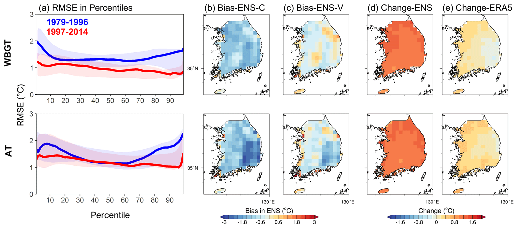
Figure 3(a) Root mean square error (RMSE; Eq. S1 in the Supplement) over the land area of South Korea in percentiles 1–99 during 1979–1996 (blue) and 1997–2014 (red). The lines and shading indicate the median and the range, respectively, of the five RCMs. (b, c) Spatial map of the bias in the 90p from ENS during the calibration (C; 1979–1996) and validation (V; 1997–2014) period, respectively. (d, e) The difference between the validation and the calibration period in 90p from ENS and ERA5, respectively. The upper row is for WBGT, and the lower row is for AT.
Figure 4 shows the median absolute error (MAE; Eq. S2 in the Supplement) over South Korea (land only) in all RCMs after BC using different methods. Two indicators – the 90p and the mean of monthly maximum (MMX) – are selected to represent extreme heat events. The diamonds standing for ENS are marked for ease of comparison. During the calibration period, LS, as the simplest BC approach used in this study, shows the largest bias among the four methods. For direct correction of WBGT, the other four methods have a reasonable MAE of less than 0.25 ∘C in the 90p and less than 0.5 ∘C in the MMX for ENS, with QDM slightly outperforming the VA and MBCn approaches. For the indirect correction, however, there is more variability among the methods and a larger bias than the direct correction. In this case, while LS still shows the worst performance, QDM presents a degraded performance, with the MAE for WBGT′ reaching 0.6 and 1.2 ∘C in the 90p and MMX, respectively. Surprisingly, VA outperforms the more advanced QM methods (i.e., QDM) in ENS, indicating the complexity of using univariate approaches to apply an indirect correction for multivariate hazards. In this case, the multivariate approach, i.e., MBCn, clearly demonstrates its strengths in such indirect correction, regardless of the indicators or periods considered. MBCn performs comparably to the direct correction of QDM during the calibration period; however, for the validation period, MBCn surpasses direct correction with an MAE of roughly 0.5 ∘C for both the 90p and MMX. In addition, MBCn shows less variability among the RCMs in WBGT′. For example, the range of MAE for WBGT′ during the calibration period as corrected by QDM is 0.38–1.23 ∘C, while that corrected by MBCn is 0.12–0.14 ∘C.
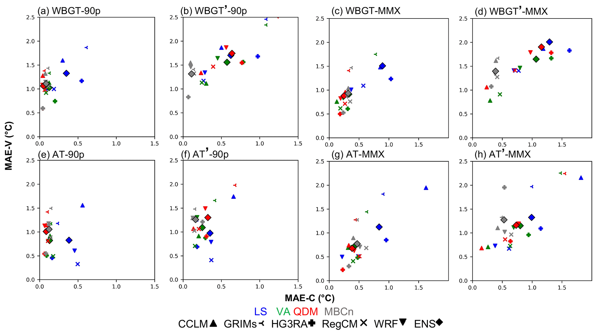
Figure 4The MAE over South Korea (land only) for the calibration period (1979–1996, x axis) and validation period (1997–2014, y axis) in terms of the (a, b, e, f) 90p and (c, d, g, h) MMX from (a, c) WBGT, (c, d) WBGT′, (e, f) TW, and (g, h) TW′. The different colors stand for different BC methods, and the different markers stand for different RCMs.
Similar results are found in AT and AT′ according to Fig. 4e–h. However, for the indirect correction of AT′, the weakness of QDM is less significant, and the advantage of MBCn is also weakened compared to WBGT′. The ability to additionally correct the multivariate dependency despite their individual distributions leads to a better result in the indirect correction of the heat-stress indices, which are functions of T and RH. In this case, since AT is more reliant than WBGT on T, the effect of correcting T–RH interdependence is less critical to its correction outcome. On the other hand, because T and RH both play important roles in WBGT, multivariate BC is more likely to demonstrate its importance in this case. Not surprisingly, the performances of different BC methods are retained in the reverse test, although with different magnitudes of MAE (Fig. S1 in the Supplement). MBCn shows an even better performance in this case, outperforming all other methods despite the heat indices and matrices considered.
To assess the quantitative differences in the marginal distributions corrected by different BC methods, Fig. 5a, b, e, and f present the maximum differences calculated from the Kolmogorov–Smirnov (K–S) test (Eq. S3) between the observed (i.e., ERA5) and bias-corrected empirical cumulative distribution functions (CDFs). A smaller value stands for a better correction output. For the direct correction, QDM and MBCn show better performances than LS and VA across all the indices and matrices considered. However, for indirect correction, MBCn shows its unique advantage in the multivariate index, depending unequally on the components (i.e., WBGT′ in this study), in that it can provide a similarly good result in either the direct or indirect correction. In this aspect, QDM shows the largest difference between the direct and indirect applications. Figure 5c, d, g, and f show the D value calculated between outputs from direct and indirect applications of the same BC method, and a smaller value stands for more similar outputs. This clearly indicates a higher similarity seen in the multivariate method than the univariate methods in WBGT, as MBCn successfully retains the inter-variable dependence during the correction procedure.
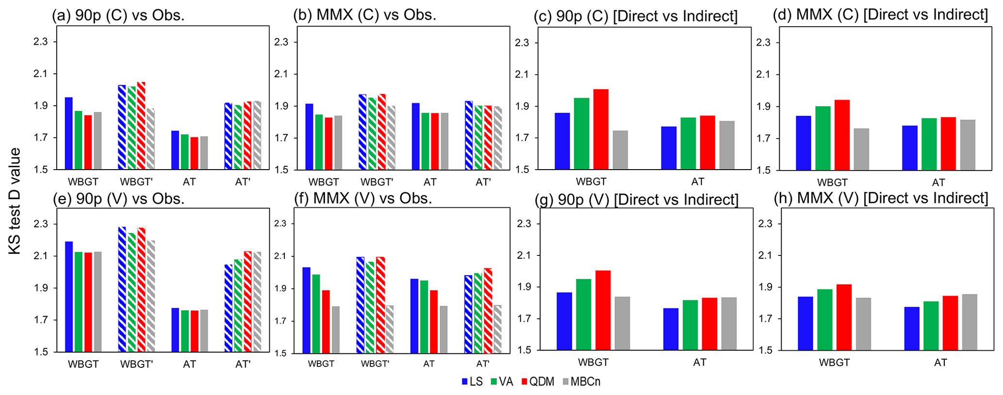
Figure 5K–S test D value between bias-corrected output and observation for (a, e) 90p and (b, f) MMX and between direct and indirect corrected output for (c, g) 90p and (d, h) MMX. The D value is the ensemble mean of five RCMs averaged over South Korea (land only). The different colors stand for different BC methods. Panels (a)–(d) are for the calibration period (C), and (e)–(h) are for the validation period (V). In (a), (b), (e), and (f), the solid and patterned fill is for the direct and indirect BC, respectively.
Figure 6 investigates the spatial distribution of bias in the QDM and MBCn corrections, using the 90p as an example for WBGT and AT. A similar pattern can also be seen in the case of MMX (Fig. S3). For the calibration period, the biases are well reduced to less than 0.5 ∘C, with only indirect correction by QDM showing a warm bias in the southeastern part. Specifically, the resultant bias magnitude from indirect QDM correction is even larger than in ORI (Fig. 3b) over southeastern Korea. The spatial pattern of the warm bias persists in the validation period, although with greater magnitude, which can be explained by the different bias magnitudes for the two periods in ORI simulations. This behavior is seen in both WBGT and AT, but more strongly in WBGT, which is more affected by the T–RH dependency. The overall cold bias in the model simulations during the calibration period must result in a positive correction coefficient (i.e., towards a warmer condition). However, as discussed above, a reduced cold bias in the RCMs is seen in the validation period because of overestimated warming in the models. Such a “trimmed” bias in the validation period may be over-corrected by the correction coefficient derived from the calibration period, even causing a larger bias than in ORI over the eastern part of the country, with a warm bias in the validation period. The results from the reverse test (Figs. 7 and S4) can further prove the impact of non-stationary bias on the result. In this case, the validation period of 1979–1996 retains a cold bias after BC for the reason that the correction coefficient derived in 1997–2014 is not large enough to compensate for its negative bias. Again, this highlights the importance of the careful interpretation of bias-corrected climate data, especially in the context of future warming projections.
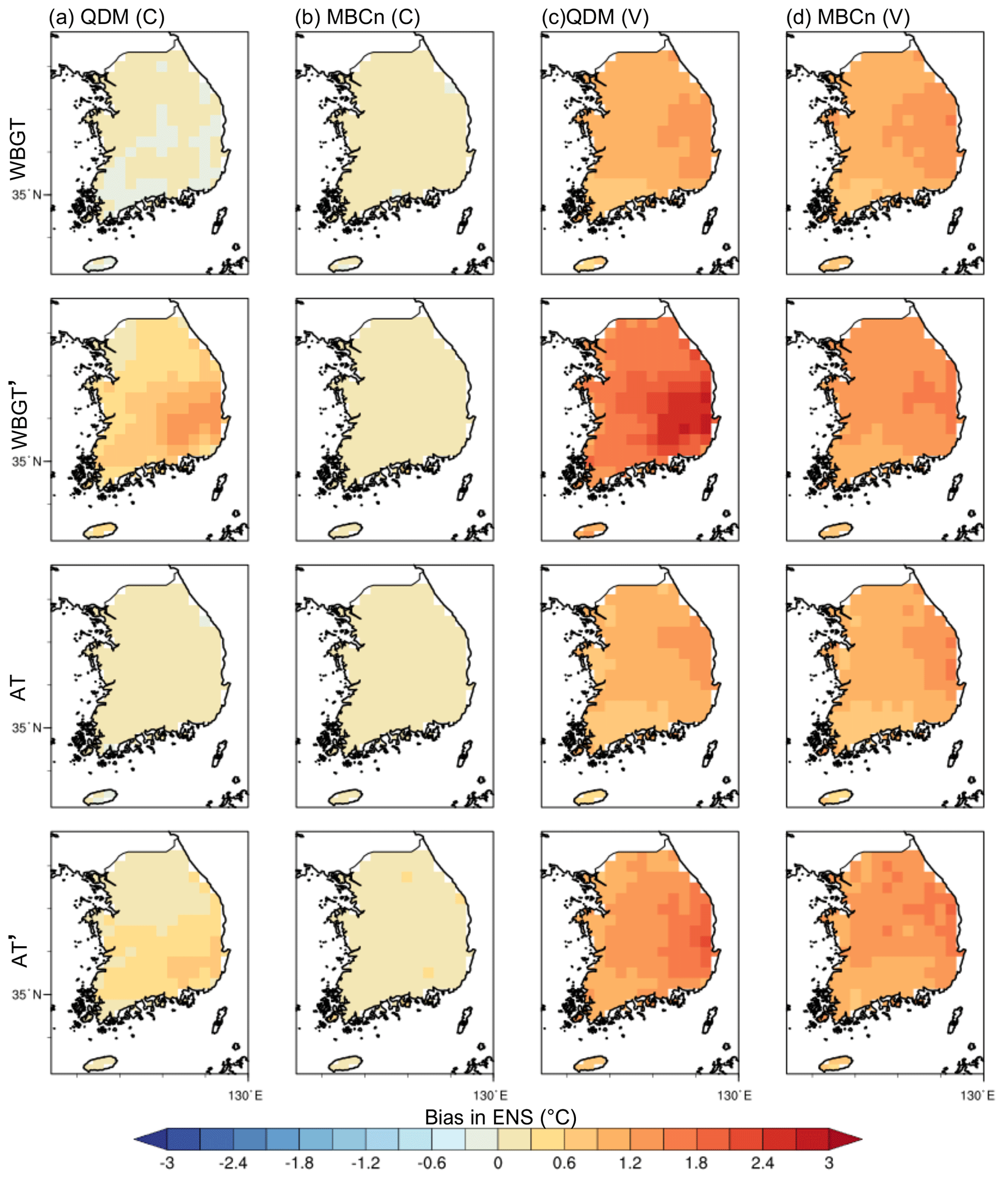
Figure 6Spatial maps of the bias in the 90p during the calibration period (C) and validation (V) period corrected by QDM and MBCn in ENS. The first and third rows are the directly corrected WBGT and AT. The second and fourth rows are the WBGT′ and AT′ calculated by the corrected T and RH.
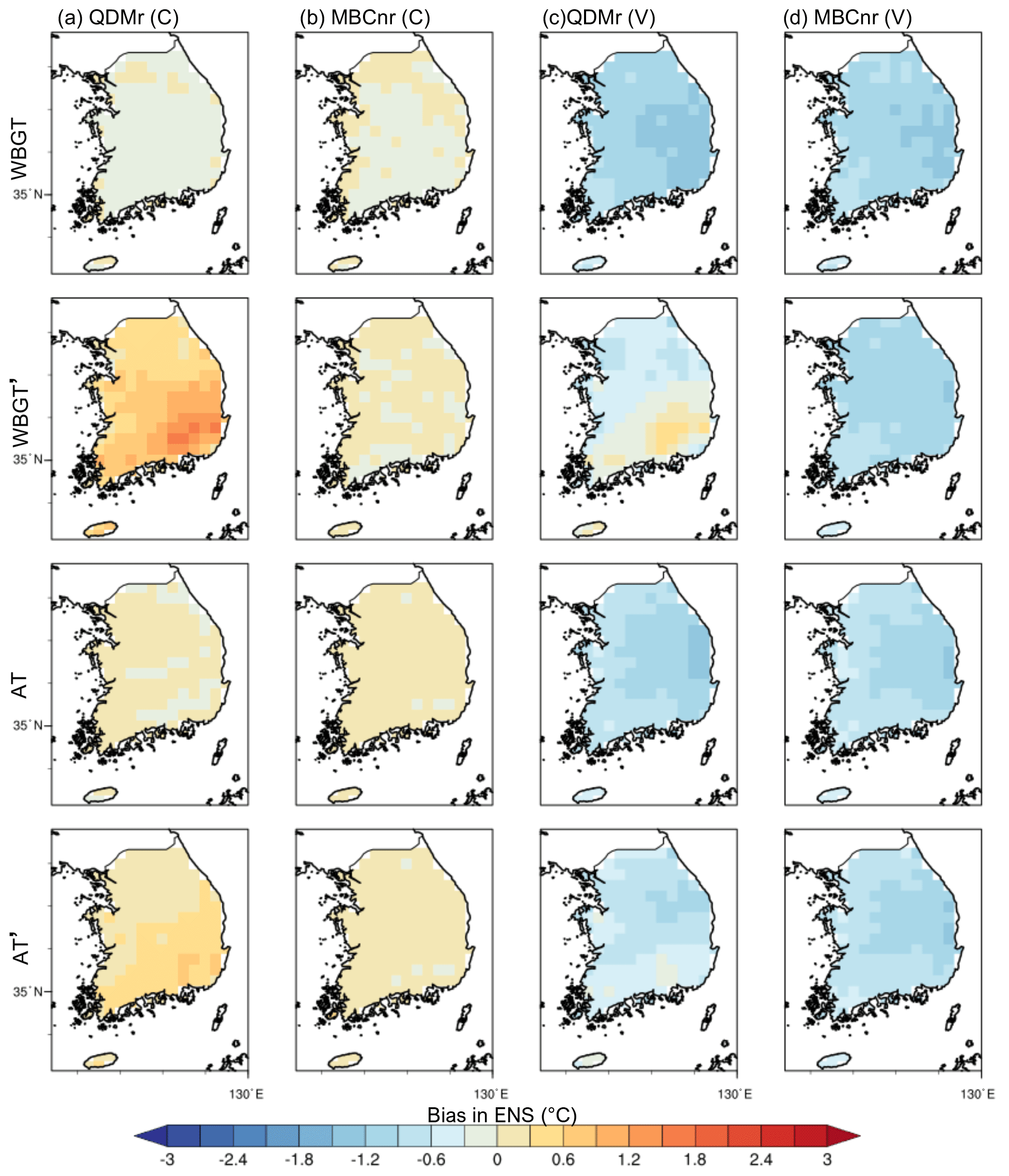
Figure 7Same as Fig. 6 but for the reverse test.
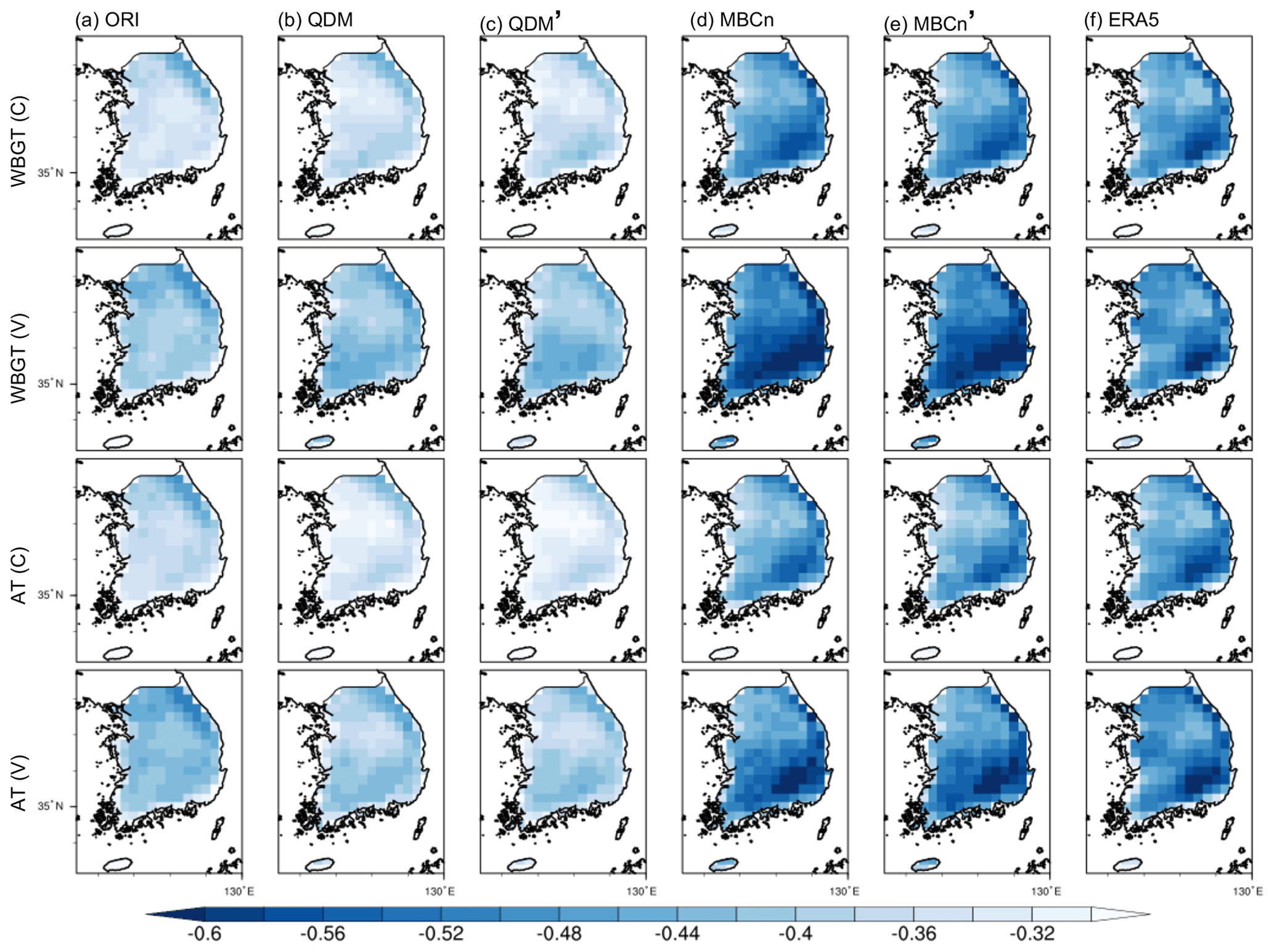
Figure 8Spatial patterns of T vs. RH Spearman's rank correlation (α=001) computed in each grid cell during the calibration (rows 1 and 3) and validation (rows 2 and 4) period. Column (a) shows the results from ORI simulations. Columns (b) and (d) are the heat-stress indices directly corrected by QDM and MBCn. Columns (c) and (e) are the heat-stress indices indirectly corrected by QDM and MBCn. Column (f) is from ERA5.
On the other hand, the spatial maps of bias also clearly demonstrate the superiority of MBCn for the indirect correction of the heat-stress indices over the entire domain in both the calibration and validation periods. Since the heat-stress indices are functions of T and RH, we investigate the T vs. RH Spearman's rank correlation at a confidence interval of 99 % using daily T and RH at the time when the heat-stress indices reach their daily maxima (Fig. 8). ERA5 shows a negative correlation ranging from −0.4 to −0.6 that gradually increases from northeast to southwest. Comparatively, ORI has a significantly weaker negative correlation and does not adequately reflect the spatial gradient. The correction with QDM, even with the good outcome in the direct correction of the heat-stress indices, cannot properly present the T–RH relation. In fact, it even further weakens their correlation during the calibration period. In contrast, MBCn calibrates the multivariate dependency according to the observed correlation pattern, which explains why it significantly improves the correction of WBGT′ and AT′. The correlation derived from the calibration period is also passed to the validation period by MBCn, which in this case shows no significant change between the two historical periods according to ERA5.
Previous studies have challenged the applicability of univariate BC for adjusting individual components of multivariate hazard indicators and proved the benefit of multivariate BC in compound event evaluations (François et al., 2020; Zscheischler et al., 2019). Our study also demonstrates MBCn's advantage in correcting the interdependence of the relevant variables, which results in a substantial improvement in the indirect BC of heat-stress indices. Such an advantage is more prominent for the index relying more equally on the composing variables (e.g., WBGT), which was also pointed out by Zscheischler et al. (2019). However, to the best of our knowledge, no study has been conducted to compare the multivariate BC methods with the direct application of univariate BC on multivariate indices. Our results show that QDM applied directly to the multivariate indices can provide a similar result to MBCn in heat-stress assessments, while MBCn additionally provides a more reasonable underlying inter-variable dependence. In this regard, if only considering heat-stress indices, the more computationally efficient direct QDM correction may be sufficient for the impact assessment. However, if the relationship between T/RH and the heat-related impacts is of interest, the multivariate BC is suggested for maintaining the physical linkage of the variables.
On the other hand, regarding the study of heat stress under future warming that is not evaluated in this study, more aspects should be considered. This study uses historical climate simulations comprising non-stationarity combined with two “jack-knifing” split-sample tests. It is found that the non-stationarity of bias in the modeled heat-stress indices, as combined effects of internal climate variability and climate model sensitivity, can significantly affect the BC output. Teutschbein and Seibert (2012) once suggested that the more advanced correction methods (e.g., QM) are more robust to a non-stationary bias compared to the simpler ones (e.g., LS), but our result shows no significant difference. In fact, lying under the fundamental assumption of stationary bias, current BC approaches may not be able to provide a suitable solution to this issue. Therefore, a case-by-case evaluation of BC approaches for a certain climate model and study area, as well as a clear understanding of the relevant processes including the uncertainties underlying original model data, is required for reliable data post-processing using BC methods. Meanwhile, for the continuous development in future projections of multivariate heat-stress indices, there are also potential problems worth investigating. For example, we may need to consider whether there is any substantial change in the modeled multivariate dependence structure, which is also highly likely under global warming (Singh et al., 2021; Hao et al., 2019). Although both QDM and MBCn are supposed to preserve the simulated trend in the corrected variables, MBCn, as well as other multivariate BC methods, does not consider the change in the multivariate relationships. In this regard, the direct correction of QDM may outperform MBCn. However, as direct correction of QDM may discard the physical consistency in the input variables, in terms of both the variable representation and the projected change, it can hide the compensating bias (Schwingshackl et al., 2021) and thus introduce additional uncertainty in climate change signal (Casanueva et al., 2018) in the multivariate heat-stress indices. To solve these problems, a deeper understanding and continuous enhancement in climate models, particularly for the uncertainty and credibility of projections, may be prerequisites for better evaluation and application of the statistical procedures (i.e., BC approaches).
Near-surface temperature and relative humidity data from the CORDEX-East domain downscaling product used in this study are archived in the institutional repository at https://doi.org/10.14711/dataset/GTXJVQ (Qiu et al., 2023). ERA5 hourly data on single levels are downloaded from the Climate Data Store via https://doi.org/10.24381/cds.adbb2d47 (Hersbach et al., 2023; ERA5 hourly data on single levels from 1979 to present). The R package “qmap” (https://CRAN.R-project.org/package=qmap; Gudmundsson, 2016) is used for applying EQM and QDM, and the R package “MBC” (https://CRAN.R-project.org/package=MBC; Cannon, 2020) is used for applying MBCn. The Climate Data Operators (CDO) open-source package is used for (1) computations in LS and VA, (2) temporal and spatial correlation, and (3) statistical analysis.
The supplement related to this article is available online at: https://doi.org/10.5194/esd-14-507-2023-supplement.
ESI and SKM conceptualized the study. LQ was responsible for investigation, formal analysis, methodology, software, and visualization. ESI supervised all LQ's work and provided investigations. LQ and ESI wrote the original draft, and ESI and SKM reviewed and edited it. LQ, SKM, YHK, DHC, SWS, JBA, ECC, and YHB created the data used in the study.
The contact author has declared that none of the authors has any competing interests.
Publisher’s note: Copernicus Publications remains neutral with regard to jurisdictional claims in published maps and institutional affiliations.
We thank the reviewers, who have provided valuable comments for the study.
This study was supported by the Korea Meteorological Administration Research and Development Program under grant no. KMI2021-00912.
This paper was edited by Sagnik Dey and reviewed by Nicholas Osborne and one anonymous referee.
ACSM: Prevention of thermal injuries during distance running: Postition stand, Med. J. Aust., 141, 876–879, https://doi.org/10.5694/j.1326-5377.1984.tb132981.x, 1984.
Bárdossy, A. and Pegram, G.: Multiscale spatial recorrelation of RCM precipitation to produce unbiased climate change scenarios over large areas and small, Water Resour. Res., 48, W09502, https://doi.org/10.1029/2011WR011524, 2012.
Cannon, A. J.: Multivariate quantile mapping bias correction: an N-dimensional probability density function transform for climate model simulations of multiple variables, Clim. Dynam., 50, 31–49, https://doi.org/10.1007/s00382-017-3580-6, 2018.
Cannon, A. J.: R package “MBC”: Multivariate Bias Correction of Climate Model Outputs, CRAN-R [code], https://CRAN.R-project.org/package=MBC (last access: 21 April 2023), 2020.
Cannon, A. J., Sobie, S. R., and Murdock, T. Q.: Bias correction of GCM precipitation by quantile mapping: How well do methods preserve changes in quantiles and extremes?, J. Climate, 28, 6938–6959, https://doi.org/10.1175/JCLI-D-14-00754.1, 2015.
Casanueva, A., Bedia, J., Herrera, S., Fernández, J., and Gutiérrez, J. M.: Direct and component-wise bias correction of multi-variate climate indices: the percentile adjustment function diagnostic tool, Climatic Change, 147, 411–425, https://doi.org/10.1007/s10584-018-2167-5, 2018.
Casanueva, A., Kotlarski, S., Herrera, S., Fischer, A. M., Kjellstrom, T., and Schwierz, C.: Climate projections of a multivariate heat stress index: the role of downscaling and bias correction, Geosci. Model Dev., 12, 3419–3438, https://doi.org/10.5194/gmd-12-3419-2019, 2019.
Chen, F. and Dudhia, J.: Coupling an advanced land surface – hydrology model with the Penn State – NCAR MM5 Modeling System. Part I: Model implementation and sensitivity, Mon. Weather Rev., 129, 569–585, https://doi.org/10.1175/1520-0493(2001)129<0569:caalsh>2.0.co;2, 2001.
Chen, J., Arsenault, R., Briquette, F., and Zhang, S.: Climate Change Impact Studies: Should We Bias Correct Climate Model Outputs or Post-Process Impact Model Outputs?, Water Resour. Res., 57, e2020WR028638, https://doi.org/10.1029/2020WR028638, 2021.
Coffel, E. D., Horton, R. M., and de Sherbinin, A.: Temperature and humidity based projections of a rapid rise in global heat stress exposure during the 21st century, Environ. Res. Lett., 13, 14001, https://doi.org/10.1088/1748-9326/aaa00e, 2017.
Dieng, D., Cannon, A. J., Laux, P., Hald, C., Adeyeri, O., Rahimi, J., Srivastava, A. K., Mbaye, M. L., and Kunstmann, H.: Multivariate bias-correction of high-resolution regional climate change simulations for West Africa: Performance and climate change implications, J. Geophys. Res.-Atmos., 127, e2021JD034836, https://doi.org/10.1029/2021JD034836, 2022.
Ehret, U., Zehe, E., Wulfmeyer, V., Warrach-Sagi, K., and Liebert, J.: HESS Opinions “Should we apply bias correction to global and regional climate model data?”, Hydrol. Earth Syst. Sci., 16, 3391–3404, https://doi.org/10.5194/hess-16-3391-2012, 2012.
François, B., Vrac, M., Cannon, A. J., Robin, Y., and Allard, D.: Multivariate bias corrections of climate simulations: which benefits for which losses?, Earth Syst. Dynam., 11, 537–562, https://doi.org/10.5194/esd-11-537-2020, 2020.
Gudmundsson, L.: R package “qmap”: Statistical Transformations for Post-Processing Climate Model Output, CRAN-R [code], https://CRAN.R-project.org/package=qmap (last access: 21 April 2023), 2016.
Gudmundsson, L., Bremnes, J. B., Haugen, J. E., and Engen-Skaugen, T.: Technical Note: Downscaling RCM precipitation to the station scale using statistical transformations – a comparison of methods, Hydrol. Earth Syst. Sci., 16, 3383–3390, https://doi.org/10.5194/hess-16-3383-2012, 2012.
Hao, Z., Phillips, T. J., Hao, F., and Wu, X.: Changes in the dependence between global precipitation and temperature from observations and model simulations, Int. J. Climatol., 39, 4895–4906, https://doi.org/10.1002/joc.6111, 2019.
Hersbach, H., Bell, B., Berrisford, P., Biavati, G., Horányi, A., Muñoz Sabater, J., Nicolas, J., Peubey, C., Radu, R., Rozum, I., Schepers, D., Simmons, A., Soci, C., Dee, D., and Thépaut, J.-N.: ERA5 hourly data on single levels from 1940 to present, Copernicus Climate Change Service (C3S) Climate Data Store (CDS) [data set], https://doi.org/10.24381/cds.adbb2d47, 2023.
Kang, S., Pal, J. S., and Eltahir, E. A. B.: Future heat stress during Muslim Pilgrimage (Hajj) projected to exceed “Extreme Danger” levels, Geophys. Res. Lett., 46, 10094–10100, https://doi.org/10.1029/2019GL083686, 2019.
Kim, G., Cha, D.-H., Lee, G., Park, C., Jin, C.-S., Lee, D.-K., Suh, M.-S., Ahn, J.-B., Min, S.-K., and Kim, J.: Projection of future precipitation change over South Korea by regional climate models and bias correction methods, Theor. Appl. Climatol., 141, 1415–1429, https://doi.org/10.1007/s00704-020-03282-5, 2020.
Kim, K. B., Kwon, H.-H., and Han, D.: Intercomparison of joint bias correction methods for precipitation and flow from a hydrological perspective, J. Hydrol., 604, 127261, https://doi.org/10.1016/j.jhydrol.2021.127261, 2022.
Kim, M.-K., Yu, D.-G., Oh, J.-S., Byun, Y.-H., Boo, K.-O., Chung, I.-U., Park, J.-S., Park, D.-S. R., Min, S.-K., and Sung, H. M.: Performance evaluation of CMIP5 and CMIP6 models on heatwaves in Korea and associated teleconnection patterns, J. Geophys. Res.-Atmos., 125, e2020JD032583, https://doi.org/10.1029/2020JD032583, 2020.
Kim, Y.-T., Kwon, H.-H., Lima, C., and Sharma, A.: A novel spatial downscaling approach for climate change assessment in regions with sparse ground data networks, Geophys. Res. Lett., 48, e2021GL095729, https://doi.org/10.1029/2021GL095729, 2021.
Lee, M., Im, E., and Bae, D.: Impact of the spatial variability of daily precipitation on hydrological projections: A comparison of GCM- and RCM-driven cases in the Han River basin, Korea, Hydrol. Process., 33, 2240–2257, https://doi.org/10.1002/hyp.13469, 2019.
Lee, M., Cha, D.-H., Suh, M.-S., Chang, E.-C., Ahn, J.-B., Min, S.-K., and Byun, Y.-H.: Comparison of tropical cyclone activities over the western North Pacific in CORDEX-East Asia phase I and II experiments, J. Climate, 1–36, https://doi.org/10.1175/JCLI-D-19-1014.1, 2020.
Maraun, D., Shepherd, T. G., Widmann, M., Zappa, G., Walton, D., Gutiérrez, J. M., Hagemann, S., Richter, I., Soares, P. M. M., Hall, A., and Mearns, L. O.: Towards process-informed bias correction of climate change simulations, Nat. Clim. Change, 7, 764–773, https://doi.org/10.1038/nclimate3418, 2017.
Masaki, Y., Hanasaki, N., Takahashi, K., and Hijioka, Y.: Propagation of biases in humidity in the estimation of global irrigation water, Earth Syst. Dynam., 6, 461–484, https://doi.org/10.5194/esd-6-461-2015, 2015.
Mehrotra, R. and Sharma, A.: Correcting for systematic biases in multiple raw GCM variables across a range of timescales, J. Hydrol., 520, 214–223, https://doi.org/10.1016/j.jhydrol.2014.11.037, 2015.
Mehrotra, R. and Sharma, A.: A multivariate quantile-matching bias correction approach with auto- and cross-dependence across multiple time scales: Implications for downscaling, J. Climate, 29, 3519–3539, https://doi.org/10.1175/JCLI-D-15-0356.1, 2016.
Meyer, J., Kohn, I., Stahl, K., Hakala, K., Seibert, J., and Cannon, A. J.: Effects of univariate and multivariate bias correction on hydrological impact projections in alpine catchments, Hydrol. Earth Syst. Sci., 23, 1339–1354, https://doi.org/10.5194/hess-23-1339-2019, 2019.
Qiu, L., Im, E.-S., Hur, J., and Shim, K.-M.: Added value of very high resolution climate simulations over South Korea using WRF modeling system, Clim. Dynam., 54, 173–189, https://doi.org/10.1007/s00382-019-04992-x, 2020.
Qiu, L., Kim, J.-B., Kim, S.-H., Choi, Y.-W., Im, E.-S., and Bae, D.-H.: Reduction of the uncertainties in the hydrological projections in Korean river basins using dynamically downscaled climate projections, Clim. Dynam., 59, 2151–2167, https://doi.org/10.1007/s00382-022-06201-8, 2022.
Qiu, L., Im, E.-S., Min, S.-K., Kim, Y.-H., Cha, D.-H., Shin, S.-W., Ahn, J.-B., Chang, E.-C., and Byun, Y.-H.: Near-surface temperature and relative humidity data from the CORDEX-East domain downscaling product over South Korea, HKUST Dataverse [data set], https://doi.org/10.14711/dataset/GTXJVQ, 2023.
Refsgaard, J. C., Madsen, H., Andréassian, V., Arnbjerg-Nielsen, K., Davidson, T. A., Drews, M., Hamilton, D. P., Jeppesen, E., Kjellström, E., Olesen, J. E., Sonnenborg, T. O., Trolle, D., Willems, P., and Christensen, J. H.: A framework for testing the ability of models to project climate change and its impacts, Climatic Change, 122, 271–282, https://doi.org/10.1007/s10584-013-0990-2, 2014.
Robin, Y., Vrac, M., Naveau, P., and Yiou, P.: Multivariate stochastic bias corrections with optimal transport, Hydrol. Earth Syst. Sci., 23, 773–786, https://doi.org/10.5194/hess-23-773-2019, 2019.
Rocheta, E., Evans, J. P., and Sharma, A.: Can bias correction of regional climate model lateral boundary conditions improve low-frequency rainfall variability?, J. Climate, 30, 9785–9806, https://doi.org/10.1175/JCLI-D-16-0654.1, 2017.
Schwingshackl, C., Sillmann, J., Vicedo-Cabrera, A. M., Sandstad, M., and Aunan, K.: Hear stress indicators in CMIP6: Estimating future trends and exceedances of impact-relevant thresholds, Earth's Future, 9, e2020EF001885, https://doi.org/10.1029/2020EF001885, 2021.
Sherwood, S. C.: How important is humidity in heat stress?, J. Geophys. Res.-Atmos., 123, 11808–11810, https://doi.org/10.1029/2018JD028969, 2018.
Singh, H., Najafi, M. R., and Cannon, A. J.: Characterizing non-stationary compound extreme events in a changing climate based on large-ensemble climate simulations, Clim. Dynam., 56, 1389–1405, https://doi.org/10.1007/s00382-020-05538-2, 2021.
Steadman, R. G.: A universal scale of apparent temperature, J. Appl. Meteorol. Clim., 23, 1674–1687, https://doi.org/10.1175/1520-0450(1984)023<1674:AUSOAT>2.0.CO;2, 1984.
Switanek, M. B., Troch, P. A., Castro, C. L., Leuprecht, A., Chang, H.-I., Mukherjee, R., and Demaria, E. M. C.: Scaled distribution mapping: a bias correction method that preserves raw climate model projected changes, Hydrol. Earth Syst. Sci., 21, 2649–2666, https://doi.org/10.5194/hess-21-2649-2017, 2017.
Teutschbein, C. and Seibert, J.: Bias correction of regional climate model simulations for hydrological climate-change impact studies: Review and evaluation of different methods, J. Hydrol., 456–457, 12–29, https://doi.org/10.1016/j.jhydrol.2012.05.052, 2012.
Vrac, M.: Multivariate bias adjustment of high-dimensional climate simulations: the Rank Resampling for Distributions and Dependences (R2D2) bias correction, Hydrol. Earth Syst. Sci., 22, 3175–3196, https://doi.org/10.5194/hess-22-3175-2018, 2018.
Zelinka, M. D., Myers, T. A., McCoy, D. T., Po-Chedley, S., Caldwell, P. M., Ceppi, P., Klein, S. A., and Taylor, K. E.: Causes of higher climate sensitivity in CMIP6 models, Geophys. Res. Lett., 47, e2019GL085782, https://doi.org/10.1029/2019GL085782, 2020.
Zscheischler, J., Fischer, E. M., and Lange, S.: The effect of univariate bias adjustment on multivariate hazard estimates, Earth Syst. Dynam., 10, 31–43, https://doi.org/10.5194/esd-10-31-2019, 2019.