the Creative Commons Attribution 4.0 License.
the Creative Commons Attribution 4.0 License.
 | 12 Apr 2023
How does the phytoplankton–light feedback affect the marine N2O inventory?
Julien Jouanno
Roland Séférian
Marion Gehlen
William Llovel
The phytoplankton–light feedback (PLF) describes the interaction between phytoplankton biomass and the downwelling shortwave radiation entering the ocean. The PLF allows the simulation of differential heating across the ocean water column as a function of phytoplankton concentration. Only one third of the Earth system models contributing to the 6th phase of the Coupled Model Intercomparison Project (CMIP6) include a complete representation of the PLF. In other models, the PLF is either approximated by a prescribed climatology of chlorophyll or not represented at all. Consequences of an incomplete representation of the PLF on the modelled biogeochemical state have not yet been fully assessed and remain a source of multi-model uncertainty in future projection. Here, we evaluate within a coherent modelling framework how representations of the PLF of varying complexity impact ocean physics and ultimately marine production of nitrous oxide (N2O), a major greenhouse gas. We exploit global sensitivity simulations at 1∘ horizontal resolution over the last 2 decades (1999–2018), coupling ocean, sea ice and marine biogeochemistry. The representation of the PLF impacts ocean heat uptake and temperature of the first 300 m of the tropical ocean. Temperature anomalies due to an incomplete PLF representation drive perturbations of ocean stratification, dynamics and oxygen concentration. These perturbations translate into different projection pathways for N2O production depending on the choice of the PLF representation. The oxygen concentration in the North Pacific oxygen-minimum zone is overestimated in model runs with an incomplete representation of the PLF, which results in an underestimation of local N2O production. This leads to important regional differences of sea-to-air N2O fluxes: fluxes are enhanced by up to 24 % in the South Pacific and South Atlantic subtropical gyres but reduced by up to 12 % in oxygen-minimum zones of the Northern Hemisphere. Our results, based on a global ocean–biogeochemical model at CMIP6 state-of-the-art level, shed light on current uncertainties in modelled marine nitrous oxide budgets in climate models.
- Article
(3609 KB) - Full-text XML
-
Supplement
(1437 KB) - BibTeX
- EndNote


-
Forced ocean–biogeochemical simulations reveal that marine production of nitrous oxide is sensitive to the representation of the phytoplankton–light feedback.
-
The phytoplankton–light feedback perturbs the accumulation of heat and the ocean dynamics, which drive changes in nitrous oxide production patterns.
-
An incomplete phytoplankton–light feedback overestimates sea-to-air N2O fluxes by up to 24 % in subtropical gyres and reduces them by up to 12 % in oxygen-minimum zones.
Feedbacks between the physical, biogeochemical or ecosystem components of the ocean can trigger abrupt system changes (Heinze et al., 2021). At present, the interactive phytoplankton–light feedback (PLF) is the only coupling in Earth system models between modelled marine biogeochemistry and ocean dynamics (Séférian et al., 2020). It implies that the chlorophyll (CHL) produced by the biogeochemical model is used to determine the fraction of shortwave radiation penetrating ocean surface waters. In this case, the CHL concentration profile used to approximate the influence of plankton biomass on the vertical redistribution of heat in the upper ocean is consistent with the one used to compute biogeochemical cycling.
1.1 Phytoplankton–light feedback (PLF)
Since the first observational evidence on how suspended matter in surface waters will impact light absorption by the ocean and change the radiative imbalance within the mixed layer (Kahru et al., 1993), this biophysical interaction has been gradually included to ocean models. Gildor and Naik (2005) highlighted the importance of considering monthly variations of CHL to capture the first-order effect of marine biota on light penetration in ocean models. Adding light–CHL interactions to numerical simulations affects oceanic processes over a wide range of spatial and temporal scales. Enabling a phytoplankton–light interaction modifies the hydrodynamics of the water column (Edwards et al., 2001, 2004), the intensity of the spring bloom in subpolar regions (Oschlies, 2004), the maintenance of the Pacific cold tongue (Anderson et al., 2007), the seasonality of the Arctic Ocean (Lengaigne et al., 2009), the strength of the tropical Pacific annual cycle, the ENSO variability (Timmermann and Jin, 2002; Marzeion et al., 2005), the northward extension of the meridional overturning circulation (Patara et al., 2012) and the cooling of the Atlantic and Peru–Chili upwelling systems (Hernandez et al., 2017; Echevin et al., 2021).
However, the mean effect of the PLF on sea surface temperature has been argued to depend on the numerical framework (forced ocean versus coupled ocean–atmosphere models). The conflicting results reported in the literature were mainly due to diverging bio-optical protocols among models rather than the inclusion of air–sea coupling. According to Park et al. (2014), atmosphere–ocean coupling amplifies the magnitude of PLF-induced changes without altering the sign of the response obtained in ocean-only simulations. Two main causes were put forward to explain the sign of the final heat perturbation: either an indirect dynamical response (Murtugudde et al., 2002; Löptien et al., 2009) or a direct thermal effect (Mignot et al., 2013; Hernandez et al., 2017). Hernandez et al. (2017) further distinguished a local from a remote thermal effect by highlighting the important role played by the advection of offshore CHL-induced cold anomalies in the Benguela upwelling waters. The interplay of these mechanisms is regionally variable (Park et al., 2014). Despite the diversity of modelled responses, a consensus emerges on the first-order effect of PLF on the ocean physics, which is to perturb the ocean thermal structure (Nakamoto et al., 2001; Murtugudde et al., 2002; Oschlies, 2004; Manizza et al., 2005, 2008; Anderson et al., 2007; Lengaigne et al., 2007; Gnanadesikan and Anderson, 2009; Löptien et al., 2009; Patara et al., 2012; Mignot et al., 2013; Hernandez et al., 2017). By trapping more heat at the ocean surface in eutrophic regions, such as coastal or equatorial upwelling areas, the presence of phytoplankton initially increases the surface warming. Confining heat at the surface leads to less heat penetrating the subsurface. In some cases, the advection and upwelling of subsurface cold anomalies can lead to remote cooling effects (Hernandez et al., 2017; Echevin et al., 2022). Dynamical readjustment in response to perturbations in thermal structure has also been shown to have a cooling effect by increasing upwelling of cold water to the ocean surface (Manizza et al., 2005; Marzeion et al., 2005; Nakamoto et al., 2001; Löptien et al., 2009; Lengaigne et al., 2007; Park et al., 2014). Because these effects depend on upper-ocean stratification, an important role is attributed to modelled seasonal deepening of the mixed layer, as it determines the intensity of the underlying temperature anomaly and its vertical movement to the surface. In other terms, whatever the temporality of the causal chain, changes in the PLF representation are expected to both perturb the ocean heat uptake and trigger perturbations of both the water column stratification and associated ocean dynamics.
1.2 This study: implications for N2O budget uncertainties
Nitrous oxide (N2O) is a major ozone-depleting substance (Ravishankara et al., 2009; Freing et al., 2012) and a potent greenhouse gas, whose global warming potential is 265–298 times that of CO2 for a 100-year timescale (Myhre et al., 2013). The spatial coherence between marine productive areas and observed hot-spots of N2O production leads one to question the impact of an incomplete representation of the PLF on the simulated N2O inventory. Recent observational studies highlight that N2O production is high in low-oxygen tropical regions and cold upwelling waters (Arévalo-Martínez et al., 2017, 2019; Yang et al., 2020; Wilson et al., 2020). N2O becomes increasingly saturated in surface waters of equatorial upwelling regions due to the upward advection of N2O-rich waters (Arévalo-Martínez et al., 2017). Regions known to account for the most productive areas of the ocean spatially coincide with highest N2O production: 64 % of the annual N2O flux occurs in the tropics, and 20 % occurs in coastal upwelling systems that occupy less than 3 % of the ocean area (Yang et al., 2020).
Despite recent advances, a large range of uncertainties still surrounds oceanic N2O emissions, as large areas of both the open and coastal ocean remain undersampled by observations (Wilson et al., 2020). In particular, the paucity of observational data over key source regions contributes to increased uncertainties. The recent global budget of Tian et al. (2020) estimates natural sources from soils and oceans to have contributed up to 57 % to the total N2O emissions between 2007 and 2016, with the ocean flux reaching 3.4 (2.5–4.3) Tg N yr−1. A large uncertainty range is associated with the ocean flux estimate, as it is based on outputs from only a small number of global ocean–biogeochemical models. Very few climate models, even in the current CMIP6 (Coupled Model Intercomparison Project phase 6) generation, include emissions (and, beforehand, a complete representation of N cycling) of N2O fluxes: only 4 out of the 26 Earth system models considered in Séférian et al. (2020) simulate marine N2O emissions.
The last generation of Earth system models projects an enhanced ocean warming in response to climate change, which is in turn expected to increase upper-ocean stratification (Sallée et al., 2021) and to contribute to greater reductions in upper-ocean nitrate and subsurface oxygen ventilation (Kwiatkowski et al., 2020). Ocean warming and deoxygenation constitute two triggers of high-probability high-impact climate tipping points (Heinze et al., 2021) and are identified as two of the main environmental factors influencing marine N2O distributions (IPCC, 2019; Hutchins and Capone, 2022). Through its expected impacts on the upper-ocean stratification, the PLF representation could further change the oceanic N2O source by modulating the mixing between N2O-rich water and intermediate depths, perturbing the way N2O-rich water reaches the air–sea interface (Freing et al., 2012).
Here, we investigate how an incomplete representation of the PLF leads to uncertainties in N2O projection in an up-to-date global ocean–biogeochemical model that makes up the current generation of Earth system models. Section 2 describes the numerical model and the set of simulations, as well as the existing options to consider CHL modulations of the incoming shortwave radiation. Section 3 presents the effect of an interactive PLF on the ocean heat content and associated ocean stratification and dynamics, as well as its feedback on marine N2O inventory. Finally, Sect. 4 summarizes the main results, addresses their broader implications and discusses the future work motivated by this study.
2.1 Configuration of the global ocean–biogeochemical model
Recent projections of future N2O emissions that contribute to intercomparison projects like CMIP6 are still based on Earth system models with a low spatial resolution (Séférian et al., 2020). For the sake of coherence with CMIP biogeochemical modelling efforts, in the following, we use a global ocean–biogeochemical configuration of the NEMO-PISCESv2 model (Madec and the NEMO System Team, 2008; Aumont et al., 2015) at 1∘ horizontal resolution. This model corresponds to the oceanic component of CNRM-ESM2-1 (Séférian et al., 2019) and is one of the few CMIP6-class models that contributed to the global N2O budget (Tian et al., 2020). Our modelled ocean has 75 vertical levels, and the first level is at 0.5 m depth. Vertical levels are unevenly spaced, with 35 levels being in the first 300 m of depth. Atmospheric forcings of momentum, incoming radiation, temperature, humidity and freshwater are provided to the ocean surface by bulk formulae following Large and Yeager (2009). Details on physical configuration are given in Berthet et al. (2019). Using an ocean-only configuration allows the local response induced by the PLF to be isolated by not confounding it with potential inter-basin feedbacks acting through the atmosphere.
JRA55-do atmospheric reanalysis (Tsujino et al., 2018, 2020) provided the atmospheric forcings of the ocean. The global domain was first spun-up under preindustrial conditions over several hundred years, ensuring that all fields approached a quasi-steady state. The historical evolution of atmospheric CO2 and N2O concentrations was prescribed from 1850. To avoid the warming jump between the end of the spin-up and the onset of the reanalyses in 1958, the first 5 years of JRA55-do forcings were cycled, followed by the complete period of JRA55-do atmospheric forcing from 1958 to 2018.
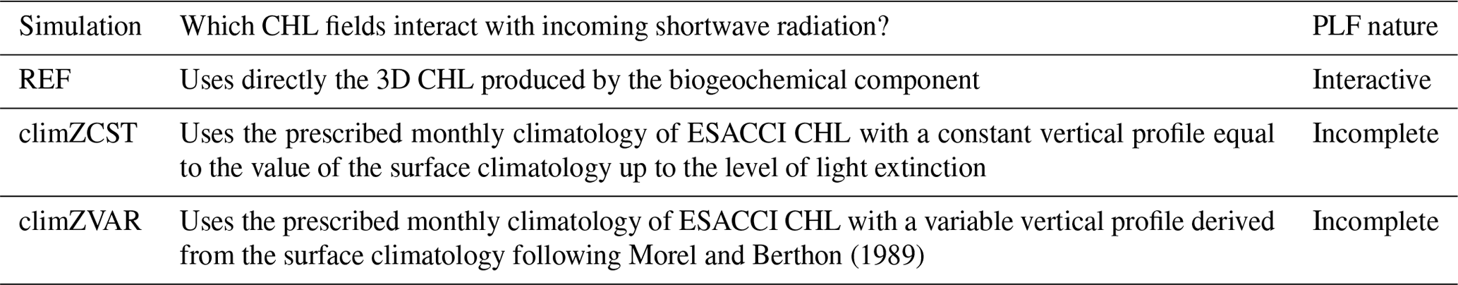
2.2 Experimental design: three representations of the PLF
The control simulation (hereafter REF) and the spin-up both account for a fully interactive PLF: the penetration of shortwave radiation into the ocean surface is constrained by the CHL concentration ([CHL]) produced by the PISCESv2 biogeochemical component (Fig. S1 in the Supplement, REF).
PISCESv2 (Pelagic Interactions Scheme for Carbon and Ecosystem Studies v2) is a 3D biogeochemical model which simulates the lower trophic levels of marine ecosystems (nanophytoplankton, diatoms, microzooplankton and mesozooplankton), as well as the biogeochemical cycles of carbon and of the main nutrients (phosphate, nitrogen, iron and silicate) along the 75 levels of our numerical ocean. A comprehensive presentation of the model is found in Aumont et al. (2015). PISCESv2 simulates prognostic 3D distributions of nanophytoplankton and diatom concentrations. The evolution of phytoplankton biomasses is the net outcome of growth, mortality, aggregation and grazing by zooplankton. The growth rate of phytoplankton mainly depends on the length of the day, depths of the mixed layer and of the euphotic zone, and the mean residence time of the cells within the unlit part of the mixed layer, and it includes a generic temperature dependency (Eppley, 1972). Nanophytoplankton growth depends on the external nutrient concentrations in nitrogen and phosphate (Monod-like parameterizations of N and P limitations) and on Fe limitation, which is modelled according to a classical quota approach. The production terms for diatoms are defined as for nanophytoplankton, except that the limitation terms also include silicate.
Light absorption by phytoplankton depends on the waveband and on the species (Bricaud et al., 1995). A simplified formulation of light absorption by the ocean is used in our experiments to calculate both the phytoplankton light limitation in PISCESv2 and the oceanic heating rate (Lengaigne et al., 2007). In this formulation, visible light is split into three wavebands: blue (400–500 nm), green (500–600 nm) and red (600–700 nm); for each waveband, the CHL-dependent attenuation coefficients, kR, kG and kB, are derived from the formulation proposed in Morel and Maritorena (2001):
where WLB means the wavelength band associated with red (R), green (G) or blue (B) and bounded by the wavelengths λ1 and λ2, as detailed above. k(λ) is the attenuation coefficient for optically pure sea water. χ(λ) and e(λ) are fitted coefficients which allow the attenuation coefficients due to chlorophyll pigments in sea water to be determined (Morel and Maritorena, 2001).

Figure 1Modelled tropical [35∘ S–35∘ N] heat content of upper 300 m (OHC300; in 1021 J (hereafter ZJ) for each simulation described in Table 1: REF (black; empty stars), climZCST (green; full downward triangles) and climZVAR (blue; empty rightward triangles). In (a), the final part of the spin-up has been added in grey to illustrate the branching protocol in year 1999, and OHC300 anomalies have been computed with respect to year 1999. Subplot (b) zooms over the Argo period to compare modelled tropical OHC300 anomalies with three in-situ-based products (see Sect. 2.3).
At year 1999, two sensitivity experiments were branched off (Fig. 1). Both simulations climZCST and climZVAR account for an incomplete and external PLF, as they consider an observed climatology of surface [CHL] from ESACCI (Valente et al., 2016) in order to compute the light penetration into sea water (Eq. 1 and Fig. S1). These two simulations differ from each other in terms of the “realism” of the vertical profile derived in each grid point from the surface value of the ESACCI CHL climatology to the level of light extinction (Table 1). climZCST uses constant profiles of CHL spreading uniformly in the vertical direction (Fig. 2b and d–f). climZVAR uses variable vertical profiles computed following Morel and Berthon (1989; Fig. 2c and d–f). This set of simulations is representative of the several configurations used in the case of CMIP intercomparison project.
In climZCST and climZVAR, PISCESv2 prognostically simulates [CHL], a key component of biogeochemical cycles, but feedback of CHL on physics (stratification, ocean heat content) is determined by the externally prescribed [CHL] climatology. The CHL concentrations used for radiation or for biogeochemical cycles are not consistent, and phytoplankton biomass computed by the biogeochemical model does not affect the physical properties of the ocean waters.
Consequences for the marine biogeochemical mean state of incomplete representations of the PLF are assessed in the following by means of difference to the control run REF. This methodology allows one to evaluate how different levels of realism and complexity in resolving bio-physical interactions impact the physical and biogeochemical content of the modelled ocean. A complete description of the marine N2O parameterization used in this model is presented in the supplementary material.

Figure 2CHL concentration (mg CHL m−3) interacting with the incoming shortwave radiation for each numerical experiment (Table 1). Maps (a–c) show annual means of the vertical sum over 0–6000 m, (a) as modelled over the 2009–2018 period for REF, and its differences in relation to the external CHL prescribed for (b) climZCST and (c) climZVAR experiments. Labels P1 to P3 on subplot (a) locate vertical profiles shown on subplots (d–f).
2.3 Observations and analyses
Model results are compared with available observation-based gridded temperature and salinity datasets. Ocean heat content (OHC) of the upper 0–300 m layer was inferred from three different products: (i) the global objective analysis of subsurface temperature EN4 (Good et al., 2013), (ii) the SIO product of the Scripps Institution of Oceanography (Roemmich and Gilson, 2009), and (iii) the ISAS20 optimal interpolation product released by Ifremer (Kolodziejczyk et al., 2019, 2021). While the SIO and ISAS20 products consider only Argo temperature and salinity profiles, the EN4 dataset considers all types of in situ profiles providing temperature and salinity (when available). These three in-situ-based datasets are considered from 2005, the year the Argo coverage became sufficient to characterize the global ocean. Details on OHC computation are given in Llovel and Terray (2016) and Llovel et al. (2022). The authors also refer to cross-validations of OHC of deeper layers (0–700 and 0–2000 m) against OHC anomalies from the World Ocean Atlas 2009 (Levitus et al., 2012). A monthly climatology (1955–2012) of oceanic temperature from the World Ocean Atlas 2013 version 2 (Locarnini et al., 2013) was used to evaluate modelled temperatures. Modelled O2 was compared to the annual climatology of O2 from the World Ocean Atlas 2013 (Garcia et al., 2014), and modelled CHL was compared to the 3D monthly climatological global product estimated from the merged satellite and hydrological data of Uitz et al. (2006). Modelled N2O partial pressure difference across the air–sea interface (Dpn2o) was compared to the recent dataset of Dpn2o observations compiled by Yang et al. (2020).
In the following, temporal means cover the last 10 years of simulations, from 2009 to 2018. In other analyses, the whole simulated period is shown (1999–2018).
3.1 Impact of PLF on the upper-ocean heat content and dynamics
Meridional sections reveal that heat perturbations in response to changing CHL fields that interact with light are limited to the top 0–300 m layer of the ocean and predominantly affect the tropical area (Figs. 3 and S2c and d in the Supplement).
The largest temperature anomalies are observed near the thermocline depth and reflect upper-ocean warming and deepening of the thermocline in climZCST (Fig. 3c) and cooling and shallowing of the thermocline in climZVAR (Fig. 3d). In climZCST, the ocean warming reflects large-scale patterns of a tropical CHL deficit compared to REF (Fig. 2b). Temperature differences are lower in the near-surface layer (0–50 m) than in the 50–300 m layer. This is expected as a result of weak stratification but also of simulations run with a forced atmosphere, in which the temperature of the ocean surface layer is constrained by the atmospheric prescribed state.
When using an incomplete representation of the PLF, two contrasting trends of the upper-ocean heat content (OHC) emerge compared to our control run REF (Fig. 1a). Over the Argo period (2005–present), EN4 estimates of tropical OHC300 are in very good agreement with our warmest simulation, climZCST (Fig. 1b), while the two other data products, SIO and ISAS20, are in better agreement with our control run REF and with climZVAR. The good accordance between modelled OHC300 and observations is not a systematic feature of model–data comparisons (Cheng et al., 2016; Liao et al., 2022). Moreover, non-negligible differences exist among OHC data products; these differences are generally particularly strong in the upper 0–300 m layer (Lyman et al., 2010; Liang et al., 2021). The spread between these products at the end of the 2005–2018 period (12.1×10²¹ J) is comparable to that of our numerical set (13.6×10²¹ J). The modelled OHC in REF is in very good agreement with current global mean in situ observations (Meyssignac et al., 2019; see their Fig. 11) and with OHC anomalies derived from the World Ocean Atlas 2009 (Levitus et al., 2012). In accordance with these observations, our ocean–biogeochemical model simulates a global mean increase of OHC over the 2006–2016 period of the order 40×1021 J for the upper 700 m and of about 70×1021 J for the 0–2000 m layer.
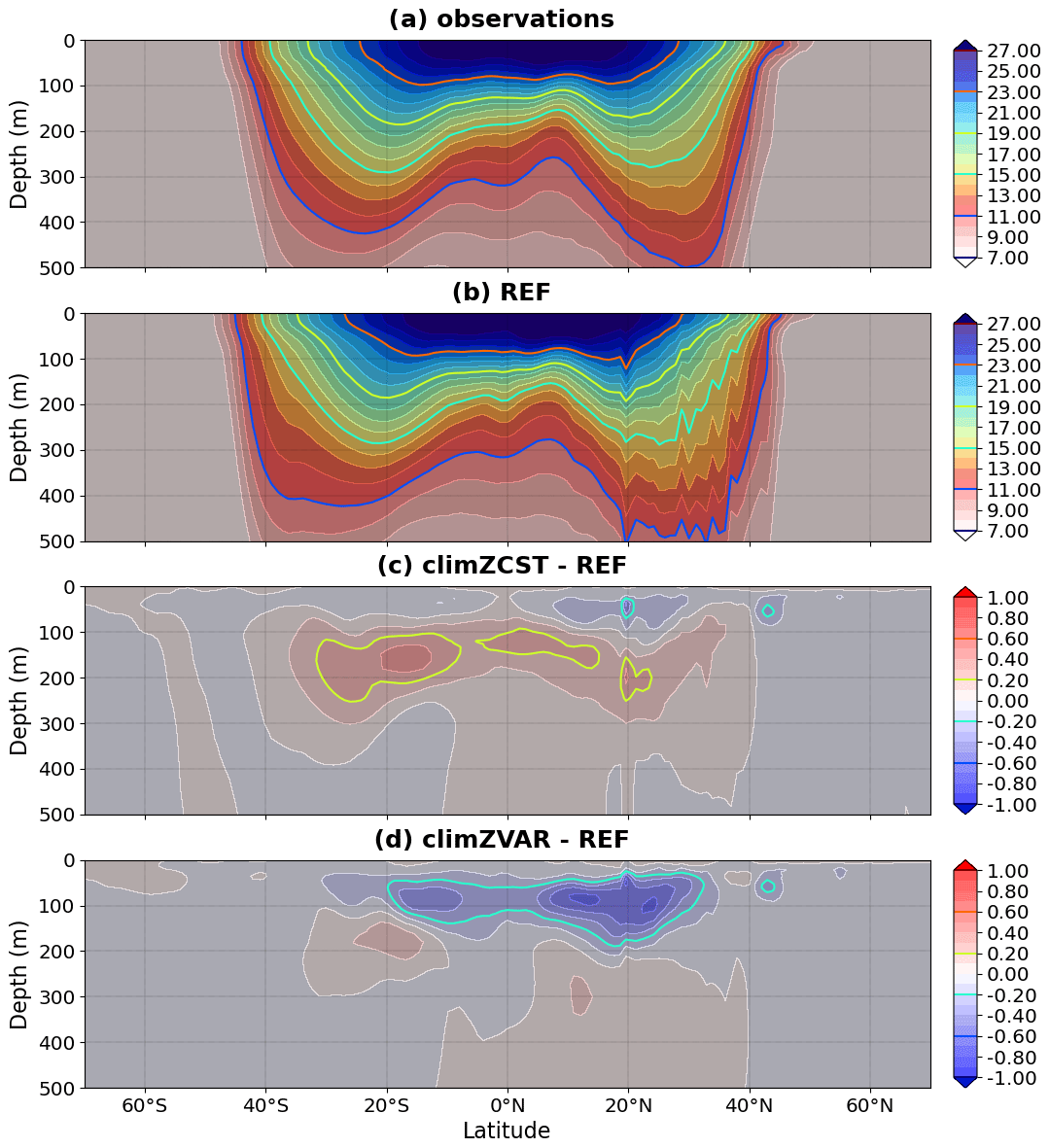
Figure 3Mean 2009–2018 meridional section of temperature (∘C) averaged over 0–360∘ E for (a) observations and (b) REF and its differences in relation to (c) climZCST and (d) climZVAR.
Subsurface thermal anomalies develop rapidly (Fig. S3 in the Supplement) after branching of climZVAR and climZCST in 1999. The dipole structure of the anomaly seen in climZCST reflects the surface heat trapping in REF and the associated subsurface cooling (Fig. S3b). Indeed, in climZCST, the vertically constant and weaker concentrations of CHL trap less incoming shortwave than the CHL maximum seen in REF between 0 and 100 m depth (Fig. 2d–f). The negative anomaly in climZVAR suggests that the parameterization of Morel and Berthon (1989) contributes to an underestimation of the ocean heat uptake (Figs. S3c and S2d) compared to REF. This heat deficit results from the overestimation of the vertical integral of CHL over large areas of the tropical domain in climZVAR compared to REF (Fig. 2c). As a result, the energy associated with the incoming radiation is caught in surface waters without being distributed over the water column.
In both climZCST and climZVAR, the subsurface temperature anomaly deepens progressively over the first 6 years of simulation as a result of vertical mixing (Fig. S3). This evolution indicates that part of the OHC300 differences between simulations comes from the adjustment of climZCST and climZVAR to the spin-up mean state yielded by an interactive PLF. It can be expected that experiments that have spin-ups run with different representations of the PLF would give even stronger sensitivities than those highlighted in this study. The sensitivities of OHC300 to the PLF formulation evaluated here should be considered at the lower end of the estimate of OHC discrepancies that may emerge from changing the PLF representation.
Prescribing a constant vertical profile of CHL (climZCST) to compute the penetration of the radiation into the ocean increases the OHC300 by more than 20×1021 J during the last 2 decades (1999–2018) compared to REF (Fig. 1). This rise of OHC300 decreases the vertically integrated tropical potential density of the upper 300 m at the end of the simulated period by 5 kg m−2 compared to REF (Fig. S4 in the Supplement). The opposite trend (a reduced OHC300 compared to REF) is simulated with the same state-of-the-art CMIP6 ocean–biogeochemical model when considering a variable vertical profile of CHL (climZVAR). However, Fig. 1 highlights that the simulation using a consistent CHL for interacting with both incoming shortwave radiation and biogeochemical cycling (REF) does not amplify one of these two trends, as climZCST and climZVAR surround REF. Average ranges of uncertainties associated with the PLF representation over the extended tropical domain (35∘ S–35∘ N) exceed 40×1021 J in terms of OHC300 (Fig. 1), 4 m for the thermocline depth and more than 9 kg m−2 for the vertically integrated potential density perturbation (Fig. S4).
Similar to OHC300, ranges of uncertainty for the OHC estimates of deeper layers (0–700 and 0–2000 m) also slightly exceed 40×1021 J. Such uncertainty ranges are quite important, as they are obtained by only changing the PLF representation in a single ocean–biogeochemical model. By comparison and in the context of OMIP protocols, Tsujino et al. (2020) give spreads between CMIP model estimates of the order of 50×1021 J for the OHC of the upper 700 m after 20 years (please refer to their Fig. 24a and b). Regarding the OHC integrated over the 0–2000 m layer, they report an inter-model spread between 50 and 100×1021 J, depending on the OMIP protocol considered (see their Fig. 24d and e). The OHC300 uncertainty of 40×1021 J triggered by the representation of the PLF in our set of simulations has a comparable order of magnitude in relation to the current spread of multi-model estimations of OHC. The present study suggests that part of the OHC multi-model uncertainty in current climate models may be due to different representations of the phytoplankton–light interaction.
The heat and associated density perturbations also cause dynamical modifications of upper-ocean currents (Fig. 4). Absolute differences in upper-ocean velocities (average between 0 and 300 m depth) are between and cm s−1, with the strongest differences along the Equator revealing perturbations of the equatorial undercurrent (Fig. 4b and c). Circulation around the subtropical gyres is also impacted, particularly for the South Pacific subtropical gyre. These modifications of zonal and meridional dynamics spread over the entire tropical latitudes, from 30∘ S to 30∘ N, strongly supporting the idea that heat perturbations induced by different interactions between CHL and incoming shortwave cause non-negligible modifications of the equatorial and tropical ocean dynamics.
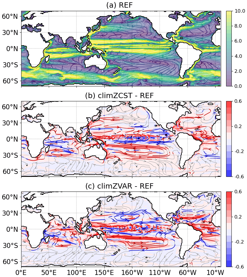
Figure 4Annual mean speed (colour; cm s−1) and streamlines of oceanic currents between 0–300 m over the 2009–2018 period for (a) REF and its differences in relation to (b) climZCST and (c) climZVAR. In (b) and (c), streamlines are coloured when absolute speed are larger than 0.05 cm s−1.
3.2 PLF impact on N2O production
Perturbations of the annual pycnocline depth (Fig. 5a–c) highlight a vertical adjustment to the heat (Fig. S2) and subsequent large-scale dynamical anomalies (Fig. 4). Variations of the pycnocline integrate perturbations of both thermal and salinity stratifications. However, in our simulations, heat anomalies appear to drive perturbations, and pycnocline depth anomalies mainly reflect those of the thermocline. The cold anomaly dominating the tropical domain in climZVAR (Fig. S2d) appears to be vertically redistributed, as it triggers an upward displacement of the isopycnals (Fig. 5c). In contrast to the anomalies seen over most of the tropical Pacific, a deepening of the isopycnals reaching up to 20 m is modelled in both the South Pacific and Atlantic subtropical gyres in climZCST and climZVAR (Fig. 5b and c). Over these subtropical gyres, heat is redistributed vertically as the subsurface warm anomaly dives. The subduction of these heat anomalies causes, in turn, a deepening of the pycnocline (Fig. 5b and c). As stressed by Sweeney et al. (2005), small changes in CHL concentration (Fig. S5 in the Supplement) may have important effects on the mixed-layer depth in these subtropical gyres due to low local wind speeds and low mixing conditions. This is thought to explain the large sensitivity we observe in terms of pycnocline depth (Fig. 5) and ocean heat content in these regions. In line with their results, our set of simulations highlights that small CHL changes in low-productivity regions trigger a vertical redistribution of density anomalies, affecting the stratification.
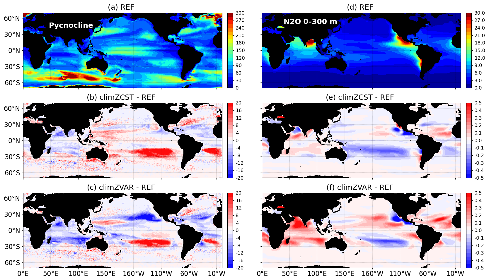
Figure 5(a–c) Depth of annual pycnocline (m) for 2009–2018 computed as the annual mean depth of the maximum of the Brunt–Väisälä frequency N2(T, S) over the water column (Maes and O'Kane, 2014). (d–f) Mean [N2O] (µmol N m−3) over the first 300 m depth. For REF (a, d) and its mean-state differences in relation to climZCST (b, e) and climZVAR (c, f).
Anomalies of N2O concentration integrated over the first 300 m of the water column (Fig. 5e and f) are in good agreement with patterns of pycnocline anomalies over the tropics (Fig. 5b and c). These comparable spatial structures attest that N2O anomalies are driven by perturbations of stratification in large parts of the tropical domain.
In the South Pacific subtropical gyre, the concomitance of (i) an increased temperature (Fig. S2c and d), (ii) a reinforced transport (Fig. 4b and c) and (iii) a weakened stratification illustrated by a local deepening of the pycnocline (Fig. 5b and c) contributes to decreasing the N2O concentration in both climZCST and climZVAR (Fig. 5e and f). In contrast, in the South Indian Ocean and North tropical Atlantic, the increase of N2O concentration seems to be mainly driven by the mean shoaling of the local pycnocline, as both regions exhibit contrasted perturbations in terms of transport and temperature. Finally, in the North Pacific oxygen-minimum zone, the strong N2O deficits in both climZCST and climZVAR compared to REF do not respond to stratification and transport anomalies but are rather driven by a local rise of O2 concentration (Fig. S6 in the Supplement). Indeed, considering an incomplete PLF in climZCST and climZVAR contributes to an overestimation of the oxygen concentration in this oxygen-minimum zone and leads to a lack of local N2O production.
The relationship between N2O concentration and OHC300 in the Tropical Ocean is derived from a linear regression for each of the three 20-year simulations (Fig. 6). The resulting slopes allow one to identify three distinct tropical N2O production pathways along time as a function of the oceanic heat uptake: from 0.3 µmol N m−2 per ZJ for the most simplified PLF scenario climZCST to 1 µmol N m−2 per ZJ for climZVAR. The slope of the simulation with the higher level of realism in terms of interactivity (REF) appears to be a solution between the two previous extremes, as it increases its N2O production by 0.8 µmol N m−2 per ZJ. Each of these N2O production pathways will translate into a different temporal evolution of the N2O budget and, hence, future climate. This result stresses the importance of having an interactive PLF in order to neither overestimate nor underestimate the N2O production projections due to a simplified representation of the PLF.
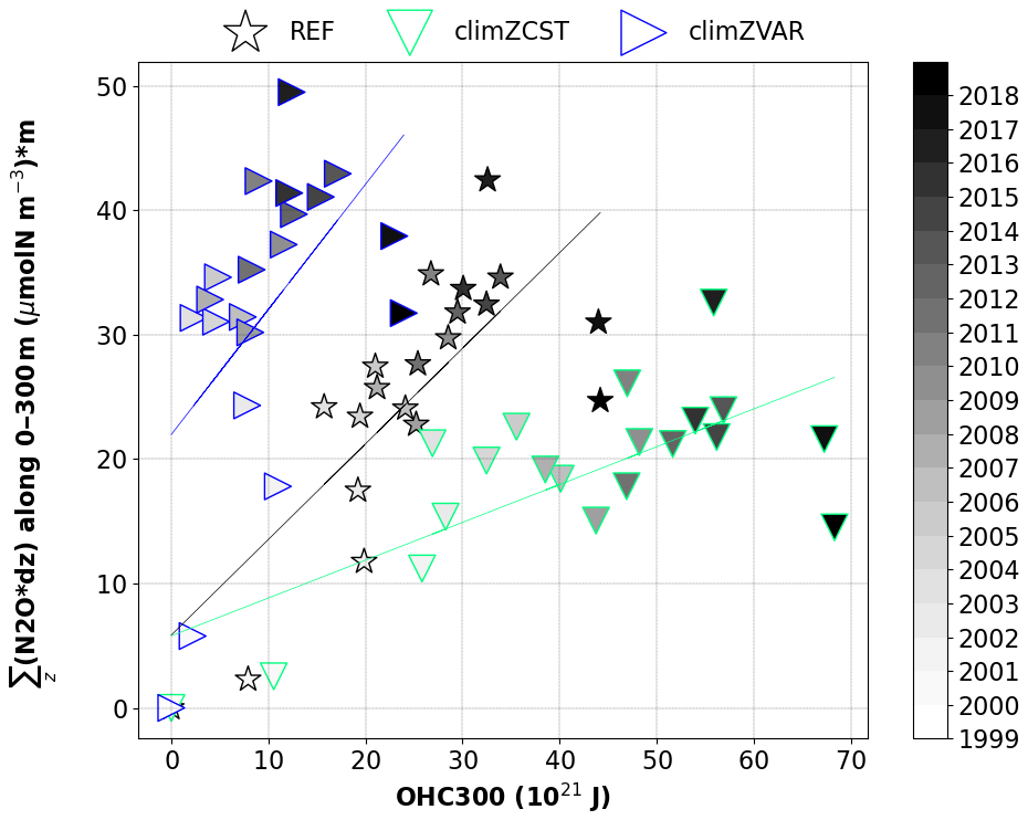
Figure 6Annual N2O inventory vertically integrated over the first 300 m depth (µmol N m−2) as a function of the annual OHC300 (ZJ) and averaged over an extended tropical domain (35∘ S–35∘ N). All points reflect anomalies compared to year 1999.
3.3 Impacts on oceanic N2O emissions
By perturbing the OHC, the ocean dynamics and the N2O production, the way PLF is modelled has non-negligible consequences on Dpn2o and thus on N2O emissions at the air–sea interface (Fig. 7). Because the atmospheric partial pressure of N2O is identical among simulations, differences in Dpn2o are driven by changes in surface oceanic N2O concentration and normalized by those in N2O solubility. Since solubility is mainly driven by temperature and because surface temperature anomalies are very weak (Fig. S3c and d), we do not expect solubility perturbations close to the surface. It results that spatial patterns of Dpn2o anomalies (Fig. 7) reflect differences in surface oceanic N2O concentration.
Compared to a scenario considering a fully interactive PLF (REF), an incomplete representation of the PLF underestimates Dpn2o in all oxygen-minimum zones of the Northern Hemisphere, which are strong emission zones (Fig. 7c and d). Large Dpn2o anomalies of −2.5 natm encompass northern parts of the oxygen-minimum zones of the Indian, Pacific and Atlantic oceans, and anomalies reach up to −5 natm locally. Consequently, climZCST and climZVAR underestimate N2O fluxes by more than 12 % in these oxygen-minimum regions compared to REF. This result highlights that the representation of the PLF can be an important source of uncertainty in modelling N2O fluxes. As a matter of fact, the oceanic contribution to the recent global N2O budget by Tian et al. (2020) is based on only five global ocean–biogeochemical models (as, still, only a few models simulate marine N2O emissions). These models have different configurations of the PLF, which adds considerable uncertainty to simulated marine N2O emissions.
In subtropical gyres, the strong and direct effect of temperature (Fig. S2c and d) on in-depth N2O concentration (Fig. 5e and f) is in line with Yang et al. (2020), who demonstrate that the seasonality of Dpn2o in those regions is driven by a solubility regime. Both climZCST and climZVAR overestimate Dpn2o in subtropical gyres of the South Pacific and South Atlantic (Fig. 7c and d). This leads to an overestimation of the regional N2O fluxes by 24 % compared to a simulation that has a complete and interactive PLF representation (REF).

Figure 7Mean sea-to-air Dpn2o (natm) computed from (a) observations and (b) REF over the 2009–2018 period and its differences in relation to (c) climZCST and (d) climZVAR.
In this study, we use the ocean component (including ocean physics, sea ice and marine biogeochemistry) of the global Earth system model CNRM-ESM2-1, which contributed to the last phase of the Coupled Model Intercomparison Project (CMIP6). Our ocean–biogeochemical model is one of the few currently able to represent an interactive phytoplankton–light feedback (PLF) by constraining the penetration of shortwave radiation into the ocean as a function of the CHL concentration produced by the biogeochemical model. Three simulations have been run at the horizontal resolution currently used for intercomparisons of Earth system models (1∘). Analyses are based on differences between a control run with an interactive PLF (REF) and two experiments with an incomplete PLF (climZCST and climZVAR) using a prescribed CHL climatology to interact with the incoming solar radiation. Changing the approach to compute how CHL filters the light penetrating into the ocean highlights the consequences of using an interactive PLF.
Our results demonstrate that the approach commonly used to account for the impact of the phytoplankton on light penetration significantly interferes with upper-ocean heat uptake (Fig. 1), as well as with the associated dynamics (Fig. 4) and stratification in the tropics (Fig. 5a–c). Our set of forced ocean–biogeochemical simulations reveals that marine production of nitrous oxide (N2O) is sensitive to the representation of the PLF (Fig. 5d–f). The heat perturbations add to the uncertainty of modelled oceanic N2O production and result in three N2O production trajectories along time (Fig. 6) that, in turn, trigger regional differences of Dpn2o and sea–air N2O fluxes (Fig. 7). Compared to an ocean model using a fully interactive PLF (REF), an incomplete PLF results in an overestimation of N2O fluxes of up to 24 % in the South Pacific and South Atlantic subtropical gyres and in a reduction of up to 12 % in oxygen-minimum zones of the Northern Hemisphere. Our results based on a state-of-the-art CMIP6 model emphasize an overlooked, important source of uncertainty in climate projections of marine N2O production and in current estimations of the marine nitrous oxide budget.
In subtropical gyres of the Southern Hemisphere, which are regions of low productivity, small CHL changes have a strong and direct effect on temperature (Fig. S2c and d), transport (Fig. 4b and c) and local stratification (Fig. 5b and c). These concomitant effects result in a local decrease of N2O concentrations in both experiments with a simplified PLF representation (climZCST and climZVAR).
In forced ocean simulations, atmospheric forcings constrain surface temperature, salinity and, thus, solubility. However, the N2O concentration integrated over the upper 300 m depth of the water column (Fig. 5e and f) showed differences in relation to the control run that follow those of the in-depth temperature (Fig. S2c and d): in climZCST (climZVAR), a warmer (colder) tropical ocean leads to a decreased (an increased) N2O concentration. Because higher marine greenhouse gas emissions will increase the temperature of the coupled atmosphere–ocean system, adding an interactive atmospheric component is expected to amplify the PLF-induced mean changes in marine N2O concentration highlighted in this ocean-only numerical set (Park et al., 2014; Asselot et al., 2022).
Our results also question the reliability of current modelled estimates of the area and volume of oxygen-minimum zones, as well as of their trends in a future climate. The expansion rate of O2-depleted waters still remains unclear, and its controlling mechanisms are not yet fully understood and represented in today's models. Observation-based assessments suggested that the ocean has already lost around 2 % of the global marine oxygen since 1960 (Schmidtko et al., 2017). The expansion of oxygen-minimum zones is expected to result in an increase of the volume of suboxic water and to have an impact on the production and decomposition of N2O (Freing et al., 2012). Our set of simulations highlights that an incomplete representation of the PLF underestimates the expansion of oxygen-depleted waters over the 20 years of simulation in comparison to REF. In climZCST and climZVAR, the global volume (0–1000 m) of hypoxic water with [O2] under 50 mmol m−3 is up to 2.3×10¹⁴ m3 lower in 2018 compared to that of the control run REF. Thus, an incomplete representation of the PLF might lead to an underestimation of 1.2 % of the modelled tropical volume of low-oxygenated waters after 20 years.
Recent regional studies demonstrated that the interactive PLF strongly affects upwelling systems of the South Pacific and Atlantic oceans (Hernandez et al., 2017; Echevin et al., 2021). Coastal upwellings are known to be sites of high N2O production, with an annual N2O flux amounting to approximately 20 % of the global fluxes, while these systems occupy less than 3 % of the ocean area (Yang et al., 2020). However, in the present study, the main modelled perturbations are rather localized over oxygen-minimum zones or subtropical gyres (Figs. 5 and 7). While the latter regional studies were performed at horizontal resolutions compatible with the complex dynamics of coastal upwellings (from 10 to about 28 km), the resolution of climate models (∼1∘ horizontal resolution) does not allow these dynamics to be resolved. A step further would be to evaluate how the sensitivity of N2O emissions to the representation of the PLF depends on the horizontal resolution by running simulations at a higher resolution with the same climate model. This would help to better determine how coastal upwelling systems may impact the modelled N2O inventory through different PLF representations, as well as the associated modelled range of uncertainty.
Sources for NEMO 3.6 and PISCESv2 code are available online at https://forge.nemo-ocean.eu/nemo (Madec and the NEMO System Team, 2008; Aumont et al., 2015).
EN4 global objective analysis of subsurface temperature is released by Met Office Hadley Centre with the following DOI: https://doi.org/10.1002/2013JC009067, and it is available online at https://hadleyserver.metoffice.gov.uk/en4/download-en4-2-2.html (Good et al., 2013). The SIO product is released by the Scripps Institution of Oceanography with the following DOI: https://doi.org/10.1016/j.pocean.2009.03.004, and it is available online at https://sio-argo.ucsd.edu/RG_Climatology.html (Roemmich and Gilson, 2009). The ISAS20 optimal interpolation product is released by Ifremer with the following DOI: https://doi.org/10.17882/52367, and it is available online at https://www.seanoe.org/data/00412/52367/ (Kolodziejczyk et al., 2019, 2021). The last access date of these datasets was in February 2022.
The supplement related to this article is available online at: https://doi.org/10.5194/esd-14-399-2023-supplement.
SB, JJ and RS conceptualized this study and its methodology. SB designed the numerical experiments, carried them out and prepared the paper with contributions from all co-authors. WL processed OHC data.
At least one of the (co-)authors is a member of the editorial board of Earth System Dynamics. The peer-review process was guided by an independent editor, and the authors also have no other competing interests to declare.
Publisher's note: Copernicus Publications remains neutral with regard to jurisdictional claims in published maps and institutional affiliations.
The OHC data were collected and made freely available by the International Argo Program and the national programmes that contribute to it. The Argo Program is part of the Global Ocean Observing System. The authors thank the two reviewers for their constructive comments and suggestions.
This project has received funding from the European Union's Horizon 2020 research and innovation programme under grant agreement no. 101003536 (ESM2025 – Earth System Models for the Future).
This paper was edited by Jadranka Sepic and reviewed by Rémy Asselot and Zarko Kovac.
Anderson, W. G., Gnanadesikan, A., Hallberg, R., Dunne, J., and Samuels, B. L.: Impact of ocean color on the maintenance of the Pacific Cold Tongue, Geophys. Res. Lett., 34, L11609, https://doi.org/10.1029/2007GL030100, 2007.
Arévalo-Martínez, D. L., Kock, A., Steinhoff, T., Brandt, P., Dengler, M., Fischer, T., Körtzinger, A., and Bange, H. W.: Nitrous oxide during the onset of the Atlantic cold tongue, J. Geophys. Res.-Oceans, 122, 171–184, https://doi.org/10.1002/2016JC012238, 2017.
Arévalo-Martínez, D. L., Steinhoff, T., Brandt, P., Körtzinger, A., Lamont, T., Rehder, G., and Bange, H. W.: N2O emissions from the northern Benguela upwelling system, Geophys. Res. Lett., 46, 3317–3326, https://doi.org/10.1029/2018GL081648, 2019.
Asselot, R., Lunkeit, F., Holden, P. B., and Hense, I.: Climate pathways behind phytoplankton-induced atmospheric warming, Biogeosciences, 19, 223–239, https://doi.org/10.5194/bg-19-223-2022, 2022.
Aumont, O., Ethé, C., Tagliabue, A., Bopp, L., and Gehlen, M.: PISCES-v2: an ocean biogeochemical model for carbon and ecosystem studies, Geosci. Model Dev., 8, 2465–2513, https://doi.org/10.5194/gmd-8-2465-2015, 2015.
Berthet, S., Séférian, R., Bricaud, C., Chevallier, M., Voldoire, A., and Ethé, C.: Evaluation of an online grid-coarsening algorithm in a global eddy-admitting ocean biogeochemical model, J. Adv. Model. Earth Sy., 11, 1759–1783, https://doi.org/10.1029/2019MS001644, 2019.
Bricaud, A., Babin, M., Morel, A., and Claustre, H.: Variability in the chlorophyll-specific absorption coefficients of natural phytoplankton: analysis and parameterization, J. Geophys. Res., 100, 13321–13332, 1995.
Cheng, L., Trenberth, K. E., Palmer, M. D., Zhu, J., and Abraham, J. P.: Observed and simulated full-depth ocean heat-content changes for 1970–2005, Ocean Sci., 12, 925–935, https://doi.org/10.5194/os-12-925-2016, 2016.
Echevin, V., Hauschildt, J., Colas, F., Thomsen, S., and Aumont, O.: Impact of chlorophyll shading on the Peruvian upwelling system, Geophys. Res. Lett., 48, e2021GL094429, https://doi.org/10.1029/2021GL094429, 2021.
Edwards, A. M., Platt, T., and Wright, D. G.: Biologically induced circulation at fronts, J. Geophys. Res., 106, 7081–7095, https://doi.org/10.1029/2000JC000332, 2001.
Edwards, A. M., Wright, D. G., and Platt, T.: Biological heating effect of a band of phytoplankton, J. Marine Syst., 49, 89–103, https://doi.org/10.1016/j.jmarsys.2003.05.011, 2004.
Eppley, R. W.: Temperature and phytoplankton growth in the sea, Fish. Bull., 70, 1063–1085, 1972.
Freing, A., Wallace, D. W. R., and Bange, H. W.: Global oceanic production of nitrous oxide, Philos. T. Roy. Soc. B, 367, 1245–1255, 2012.
Garcia, H. E., Locarnini, R. A., Boyer, T. P., Antonov, J. I., Baranova, O. K., Zweng, M. M., Reagan, J. R., and Johnson, D. R.: World Ocean Atlas 2013, Volume 3: Dissolved Oxygen, Apparent Oxygen Utilization, and Oxygen Saturation, edited by: Levitus, S. (Ed.), and Mishonov, A. (Technical Ed.), NOAA Atlas NESDIS 75, 27 pp., https://doi.org/10.7289/V5XG9P2W, 2014.
Gildor, H. and Naik, N. H.: Evaluating the effect of interannual variations of surface chlorophyll on upper ocean temperature, J. Geophys. Res., 110, C07012, https://doi.org/10.1029/2004JC002779, 2005.
Gnanadesikan, A. and Anderson, W. G.: Ocean water clarity and the ocean general circulation in a coupled climate model, J. Phys. Oceanogr., 39, 314–332, 2009.
Good, S. A., Martin, M. J., and Rayner, N. A.: EN4: Quality controlled ocean temperature and salinity profiles and monthly objective analyses with uncertainty estimates, J. Geophys. Res.-Oceans, 118, 6704–6716, https://doi.org/10.1002/2013JC009067, 2013 (data available at: https://hadleyserver.metoffice.gov.uk/en4/download-en4-2-2.html, last access: February 2022).
Heinze, C., Blenckner, T., Martins, H., Rusiecka, D., Döscher, R., Gehlen, M., Gruber, N., Holland, E., Hov, Ø., Joos, F., Matthews, J. B. R., Rødven, R., and Wilson, S.: The quiet crossing of ocean tipping points, P. Natl. Acad. Sci. USA, 118, e2008478118, https://doi.org/10.1073/pnas.2008478118, 2021.
Hernandez, O., Jouanno, J., Echevin, V., and Aumont, O.: Modification of sea surface temperature by chlorophyll concentration in the Atlantic upwelling systems, J. Geophys. Res.-Oceans, 122, 5367–5389, https://doi.org/10.1002/2016JC012330, 2017.
Hutchins, D. A. and Capone, D. G.: The marine nitrogen cycle: new developments and global change, Nat. Rev. Microbiol., 20, 401–414, https://doi.org/10.1038/s41579-022-00687-z, 2022.
IPCC: Summary for Policymakers, in: IPCC Special Report on the Ocean and Cryosphere in a Changing Climate, edited by: Pörtner, H.-O., Roberts, D. C., Masson-Delmotte, V., Zhai, P., Tignor, M., Poloczanska, E., Mintenbeck, K., Nicolai, M., Okem, A., Petzold, J., Rama, B., and Weyer, N., Cambridge University Press, Cambridge, UK and New York, NY, USA, 3–35, https://doi.org/10.1017/9781009157964.001, 2019.
Kahru, M., Leppaenen, J.-M., and Rud, O.: Cyanobacterial blooms cause heating of the sea surface, Mar. Ecol. Prog. Ser., 101, 1–7, 1993.
Kolodziejczyk, N., Llovel, W., and Portela, E.: Interannual variability of upper ocean water masses as inferred from Argo Array, J. Geophys. Res.-Oceans, 124, 6067–6085, https://doi.org/10.1029/2018JC014866, 2019.
Kolodziejczyk, N., Prigent-Mazella, A., and Gaillard, F.: ISAS temperature and salinity gridded fields, SEANOE, https://doi.org/10.17882/52367, 2021 (data available at: https://www.seanoe.org/data/00412/52367/, last access: February 2022).
Kwiatkowski, L., Torres, O., Bopp, L., Aumont, O., Chamberlain, M., Christian, J. R., Dunne, J. P., Gehlen, M., Ilyina, T., John, J. G., Lenton, A., Li, H., Lovenduski, N. S., Orr, J. C., Palmieri, J., Santana-Falcón, Y., Schwinger, J., Séférian, R., Stock, C. A., Tagliabue, A., Takano, Y., Tjiputra, J., Toyama, K., Tsujino, H., Watanabe, M., Yamamoto, A., Yool, A., and Ziehn, T.: Twenty-first century ocean warming, acidification, deoxygenation, and upper-ocean nutrient and primary production decline from CMIP6 model projections, Biogeosciences, 17, 3439–3470, https://doi.org/10.5194/bg-17-3439-2020, 2020.
Large, W. G. and Yeager, S.: The global climatology of an interannually varying air-sea flux data set, Clim. Dynam., 33, 341–364, https://doi.org/10.1007/s00382-008-0441-3, 2009.
Lengaigne, M., Menkes, C., Aumont, O., Gorgues, T., Bopp, L., André, J.-M., and Madec, G.: Influence of the oceanic biology on the tropical Pacific climate in a coupled general circulation model, Clim. Dynam., 28, 503–516, https://doi.org/10.1007/s00382-006-0200-2, 2007.
Lengaigne, M., Madec, G., Bopp, L., Menkes, C., Aumont, O., and Cadule, P.: Bio-physical feedbacks in the Arctic Ocean using an Earth system model, Geophys. Res. Lett., 36, L21602, https://doi.org/10.1029/2009GL040145, 2009.
Levitus, S., Antonov, J. I., Boyer, T. P., Baranova, O. K., Garcia, H. E., Locarnini, R. A., Mishonov, A. V., Reagan, J. R., Seidov, D., Yarosh, E. S., and Zweng, M. M.: World Ocean heat content and thermosteric sea level change (0–2000 m) 1955–2010, Geophys. Res. Lett., 39, L10603, https://doi.org/10.1029/2012GL051106, 2012.
Liang, X., Liu, C. R., Ponte, M., and Chambers, D. P.: A Comparison of the Variability and Changes in Global Ocean Heat Content from Multiple Objective Analysis Products During the Argo Period, J. Climate, 34, 7875–7895, https://doi.org/10.1175/JCLI-D-20-0794.1, 2021.
Liao, F., Wang, X. H., and Liu, Z.: Comparison of ocean heat content estimated using two eddy-resolving hindcast simulations based on OFES1 and OFES2, Geosci. Model Dev., 15, 1129–1153, https://doi.org/10.5194/gmd-15-1129-2022, 2022.
Llovel, W. and Terray, L.: Observed southern upper-ocean warming over 2005–2014 and associated mechanisms, Environ. Res. Lett., 11, 124023, https://doi.org/10.1088/1748-9326/11/12/124023, 2016.
Llovel, W., Kolodziejczyk, N., Close, S., Penduff, T., Molines, J.-M., and Terray, L.: Imprint of intrinsic ocean variability on decadal trends of regional sea level and ocean heat content using synthetic profiles, Environ. Res. Lett., 17, 044063, https://doi.org/10.1088/1748-9326/ac5f93, 2022.
Locarnini, R. A., Mishonov, A. V., Antonov, J. I., Boyer, T. P., Garcia, H. E., Baranova, O. K., Zweng, M. M., Paver, C. R., Reagan, J. R., Johnson, D. R., Hamilton, M., and Seidov, D.: World Ocean Atlas 2013, vol. 1: Temperature, edited by: Levitus, S. and Mishonov, A. (Technical Ed.), NOAA Atlas NESDIS 73, 40 pp., https://doi.org/10.7289/V55X26VD, 2013.
Löptien, U., Eden, C., Timmermann, A., and Dietze, H.: Effects of biologically induced differential heating in an eddy-permitting coupled ocean-ecosystem model, J. Geophys. Res., 114, C06011, https://doi.org/10.1029/2008JC004936, 2009.
Lyman, J. M., Good, S. A., Gouretski, V. V., Ishii, M., Johnson, G. C., Palmer, M. D., Smith, D. M., and Willis, J. K.: Robust warming of the global upper ocean, Nature, 465, 334–337, https://doi.org/10.1038/nature09043, 2010.
Madec, G. and NEMO System Team: NEMO ocean engine, Scientific Notes of Climate Modelling Center, 27, Institut Pierre-Simon Laplace (IPSL), ISSN 1288-1619, https://doi.org/10.5281/zenodo.6334656, 2008 (code available at: https://forge.nemo-ocean.eu/nemo, last access: February 2022).
Maes, C. and O'Kane, T. J.: Seasonal variations of the upper ocean salinity stratification in the Tropics, J. Geophys. Res.-Oceans, 119, 1706–1722, https://doi.org/10.1002/2013JC009366, 2014.
Manizza, M., Le Quéré, C., Watson, A. J., and Buitenhuis, E. T.: Bio-optical feedbacks among phytoplankton, upper ocean physics and sea-ice in a global model, Geophys. Res. Lett., 32, L05603, https://doi.org/10.1029/2004GL020778, 2005.
Manizza, M., Le Quéré, C., Watson, A. J., and Buitenhuis, E. T.: Ocean biogeochemical response to phytoplankton-light feedback in a global model, J. Geophys. Res., 113, C10010, https://doi.org/10.1029/2007JC004478, 2008.
Marzeion, B., Timmermann, A., Murtugudde, R., and Jin, F.: Biophysical Feedbacks in the Tropical Pacific, J. Climate, 18, 58–70, 2005.
Meyssignac, B., Boyer, T., Zhao, Z., Hakuba, M. Z., Landerer, F. W., Stammer, D., Köhl, A., Kato, S., L'Ecuyer, T., Ablain, M., Abraham, J. P., Blazquez, A., Cazenave, A., Church, J. A., Cowley, R., Cheng, L., Domingues, C. M., Giglio, D., Gouretski, V., Ishii, M., Johnson, G. C., Killick, R. E., Legler, D., Llovel, W., Lyman, J., Palmer, M. D., Piotrowicz, S., Purkey, S. G., Roemmich, D., Roca, R., Savita, A., von Schuckmann, K., Speich, S., Stephens, G., Wang, G., Wijffels, S. E., and Zilberman, N.: Measuring Global Ocean Heat Content to Estimate the Earth Energy Imbalance, Front. Mar. Sci., 6, 432, https://doi.org/10.3389/fmars.2019.00432, 2019.
Mignot, J., Swingedouw, D., Deshayes, J., Marti, O., Talandier, C., Séférian, R., Lengaigne, M., and Madec, G.: On the evolution of the oceanic component of the IPSL climate models from CMIP3 to CMIP5: A mean state comparison, Ocean Model., 72, 167–184, https://doi.org/10.1016/j.ocemod.2013.09.001, 2013.
Morel, A. and Berthon, J.-F.: Surface pigments, algal biomass profiles, and potential production of the euphotic layer: Relationships reinvestigated in view of remote-sensing applications, Limnol. Oceanogr., 34, 1545–1562, 1989.
Morel, A. and Maritorena, S.: Bio-optical properties of oceanic waters: a reappraisal, J. Geophys. Res., 106, 7163–7180, 2001.
Murtugudde, R., Beauchamp, J., McClain, C. R., Lewis, M., and Busalacchi, A. J.: Effects of Penetrative Radiation on the Upper Tropical Ocean Circulation, J. Climate, 15, 470–486, 2002.
Myhre, G., Shindell, D., Bréon, F.-M., Collins, W., Fuglestvedt, J., Huang, J., Koch, D., Lamarque, J.-F., Lee, D., Mendoza, B., Nakajima, T., Robock, A., Stephens, G., Takemura, T., and Zhang, H.: Anthropogenic and Natural Radiative Forcing, in: Climate Change 2013: The Physical Science Basis. Contribution of Working Group I to the Fifth Assessment Report of the Intergovernmental Panel on Climate Change, edited by: Stocker, T. F., Qin, D., Plattner, G.-K., Tignor, M., Allen, S. K., Boschung, J., Nauels, A., Xia, Y., Bex, V., and Midgley, P. M., Cambridge University Press, Cambridge, United Kingdom and New York, NY, USA, https://doi.org/10.1017/CBO9781107415324, 2013.
Nakamoto, S., Kumar, S. P., Oberhuber, J. M., Ishizaka, J., Muneyama, K., and Frouin, R.: Response of the equatorial Pacific to chlorophyll pigment in a mixed layer isopycnical ocean general circulation model, Geophys. Res. Lett., 28, 2021–2024, 2001.
Oschlies, A.: Feedbacks of biotically induced radiative heating on upper-ocean heat budget, circulation, and biological production in a coupled ecosystem-circulation model, J. Geophys. Res., 109, C12031, https://doi.org/10.1029/2004JC002430, 2004.
Park, J.-Y., Kug, J.-S., Seo, H., and Bader, J.: Impact of bio-physical feedbacks on the tropical climate in coupled and uncoupled GCMs, Clim. Dynam., 43, 1811–1827, https://doi.org/10.1007/s00382-013-2009-0, 2014.
Patara, L., Vichi, M., Masina, S., Fogli, P. G., and Manzini, E.: Global response to solar radiation absorbed by phytoplankton in a coupled climate model, Clim. Dynam., 39, 1951–1968, https://doi.org/10.1007/s00382-012-1300-9, 2012.
Ravishankara, A. R., Daniel, J. S., and Portmann, R. W.: Nitrous oxide (N2O): The dominant ozone-depleting substance emitted in the 21st century, Science, 326, 123–125, 2009.
Roemmich, D. and Gilson, J.: The 2004–2008 mean and annual cycle of temperature, salinity, and steric height in the global ocean from the Argo Program, Prog. Oceanogr., 82, 81–100, https://doi.org/10.1016/j.pocean.2009.03.004, 2009 (data available at: https://sio-argo.ucsd.edu/RG_Climatology.html, last access: February 2022).
Sallée, J.-B., Pellichero, V., Akhoudas, C., Pauthenet, E., Vignes, L., Schmidtko, S., Garabato, A. N., Sutherland, P., and Kuusela, M.: Summertime increases in upper-ocean stratification and mixed-layer depth, Nature, 591, 592–598, https://doi.org/10.1038/s41586-021-03303-x, 2021.
Schmidtko, S., Stramma, L., and Visbeck, M.: Decline in global oceanic oxygen content during the past five decades, Nature, 542, 335–339, 2017.
Séférian, R., Nabat, P., Michou, M., Saint-Martin, D., Voldoire, A., Colin, J., Decharme, B., Delire, C., Berthet, S., Chevallier, M., Sénési, S., Franchisteguy, L., Vial, J., Mallet, M., Joetzer, E., Geoffroy, O., Guérémy, J.-F., Moine, M.-P., Msadek, R., Ribes, A., Rocher, M., Roehrig, R., Salas-y-Mélia, D., Sanchez, E., Terray, L., Valcke, S., Waldman, R., Aumont, O., Bopp, L., Dehayes, J., Ethé, C., and Madec, G.: Evaluation of CNRM Earth-System model, CNRM-ESM2-1: role of Earth system processes in present-day and future climate, J. Adv. Model. Earth Sy., 11, 4182–4227, https://doi.org/10.1029/2019MS001791, 2019.
Séférian, R., Berthet, S., Yool, A., Palmiéri, J., Bopp, L., Tagliabue, A., Kwiatkwski, L., Aumont, O., Christian, J., Dunne, J., Gehlen, M., Ilyina, T., John, J. G., Li, H., Long, M. C., Luo, J. Y., Nakano, H., Romanou, A., Schwinger, J., Stock, C., Santana-Falcon, Y., Takano, Y., Tjiputra, J., Tsujino, H., Watanabe, M., Wu, F., and Yamamoto, A.: Tracking Improvement in Simulated Marine Biogeochemistry Between CMIP5 and CMIP6, Curr. Clim. Change Rep., 6, 95–119, https://doi.org/10.1007/s40641-020-00160-0, 2020.
Sweeney, C., Gnanadesikan, A., Griffies, S. M., Harrison, M. J., Rosati, A. J., and Samuels, B. L.: Impacts of Shortwave Penetration Depth on Large-Scale Ocean Circulation and Heat Transport, J. Phys. Oceanogr., 35, 1103–1119, 2005.
Tian, H., Xu, R., Canadell, J. G., Thompson, R. L., Winiwarter, W., Suntharalingam, P., Davidson, E. A., Ciais, P., Jackson, R. B., Janssens-Maenhout, G., Prather, M. J., Regnier, P., Pan, N., Pan, S., Peters, G., Shi, H., Tubiello, F. N., Zaehle, S., Zhou, F., Arneth, A., Battaglia, G., Berthet, S., Bopp, L., Bouwman, A. F., Buitenhuis, E. T., Chang, J., Chipperfield, M. P., Dangal, S. R. S., Dlugokencky, E., Elkins, J., Eyre, B. D., Fu, B., Hall, B., Ito, A., Joos, F., Krummel, P. B., Landolfi, A., Laruelle, G. G., Lauerwald, R., Li, W., Lienert, S., Maavara, T., MacLeod, M., Millet, D. B., Olin, S., Patra, P. K., Prinn, R. G., Raymond, P. A., Ruiz, D. J., van der Werf, G. R., Vuichard, N., Wang, J., Weiss, R., Wells, K. C., Wilson, C., Yang, J., and Yao, Y.: A comprehensive quantification of global nitrous oxide sources and sinks, Nature, 586, 248–256, https://doi.org/10.1038/s41586-020-2780-0, 2020.
Timmermann, A. and Jin, F.-F.: Phytoplankton influences on tropical climate, Geophys. Res. Lett., 29, 2104, https://doi.org/10.1029/2002GL015434, 2002.
Tsujino, H., Urakawa, S., Nakano, H., Small, R. J., Kim, W. M., Yeager, S. G., Danabasoglu, G., Suzuki, T., Bamber J. L., Bentsen, M., Böning, C. W., Bozec, A., Chassignet, E. P., Curchitser, E., Boeira Dias, F., Durack, P. J., Griffies, S. M., Harada, Y., Ilicak, M., Josey, S. A., Kobayashi, C., Kobayashi, S., Komuro, Y., Large, W. G., Le Sommer, J., Marsland, S. J., Masina, S., Scheinert, M., Tomita, H., Valdivieso, M., and Yamazaki, D.: JRA-55 based surface dataset for driving ocean–sea-ice models (JRA55-do), Ocean Model., 130, 79–139, https://doi.org/10.1016/j.ocemod.2018.07.002, 2018.
Tsujino, H., Urakawa, L. S., Griffies, S. M., Danabasoglu, G., Adcroft, A. J., Amaral, A. E., Arsouze, T., Bentsen, M., Bernardello, R., Böning, C. W., Bozec, A., Chassignet, E. P., Danilov, S., Dussin, R., Exarchou, E., Fogli, P. G., Fox-Kemper, B., Guo, C., Ilicak, M., Iovino, D., Kim, W. M., Koldunov, N., Lapin, V., Li, Y., Lin, P., Lindsay, K., Liu, H., Long, M. C., Komuro, Y., Marsland, S. J., Masina, S., Nummelin, A., Rieck, J. K., Ruprich-Robert, Y., Scheinert, M., Sicardi, V., Sidorenko, D., Suzuki, T., Tatebe, H., Wang, Q., Yeager, S. G., and Yu, Z.: Evaluation of global ocean–sea-ice model simulations based on the experimental protocols of the Ocean Model Intercomparison Project phase 2 (OMIP-2), Geosci. Model Dev., 13, 3643–3708, https://doi.org/10.5194/gmd-13-3643-2020, 2020.
Uitz, J., Claustre, H., Morel, A., and Hooker, S. B.: Vertical distribution of phytoplankton communities in open ocean: An assessment based on surface chlorophyll, J. Geophys. Res., 111, C08005, https://doi.org/10.1029/2005JC003207, 2006.
Valente, A., Sathyendranath, S., Brotas, V., Groom, S., Grant, M., Taberner, M., Antoine, D., Arnone, R., Balch, W. M., Barker, K., Barlow, R., Bélanger, S., Berthon, J.-F., Beşiktepe, Ş., Brando, V., Canuti, E., Chavez, F., Claustre, H., Crout, R., Frouin, R., García-Soto, C., Gibb, S. W., Gould, R., Hooker, S., Kahru, M., Klein, H., Kratzer, S., Loisel, H., McKee, D., Mitchell, B. G., Moisan, T., Muller-Karger, F., O'Dowd, L., Ondrusek, M., Poulton, A. J., Repecaud, M., Smyth, T., Sosik, H. M., Twardowski, M., Voss, K., Werdell, J., Wernand, M., and Zibordi, G.: A compilation of global bio-optical in situ data for ocean-colour satellite applications, Earth Syst. Sci. Data, 8, 235–252, https://doi.org/10.5194/essd-8-235-2016, 2016.
Wilson, S. T., Al-Haj, A. N., Bourbonnais, A., Frey, C., Fulweiler, R. W., Kessler, J. D., Marchant, H. K., Milucka, J., Ray, N. E., Suntharalingam, P., Thornton, B. F., Upstill-Goddard, R. C., Weber, T. S., Arévalo-Martínez, D. L., Bange, H. W., Benway, H. M., Bianchi, D., Borges, A. V., Chang, B. X., Crill, P. M., del Valle, D. A., Farías, L., Joye, S. B., Kock, A., Labidi, J., Manning, C. C., Pohlman, J. W., Rehder, G., Sparrow, K. J., Tortell, P. D., Treude, T., Valentine, D. L., Ward, B. B., Yang, S., and Yurganov, L. N.: Ideas and perspectives: A strategic assessment of methane and nitrous oxide measurements in the marine environment, Biogeosciences, 17, 5809–5828, https://doi.org/10.5194/bg-17-5809-2020, 2020.
Yang, S., Chang, B. X., Warner, M. J., Weber, T. S., Bourbonnais, A. M., Santoro, A. E., Kock, A., Sonnerup, R. E., Bullister, J. L., Wilson, S. T., and Bianchi, D.: Global reconstruction reduces the uncertainty of oceanic nitrous oxide emissions and reveals a vigorous seasonal cycle, P. Natl. Acad. Sci. USA, 117, 11954–11960, https://doi.org/10.1073/pnas.1921914117, 2020.