Time-varying changes and uncertainties in the CMIP6 ocean carbon sink from global to local scale

As a major sink for anthropogenic carbon, the oceans slow the increase in carbon dioxide in the atmosphere and regulate climate change. Future changes in the ocean carbon sink, and its uncertainty at a global and regional scale, are key to understanding the future evolution of the climate. Here we report on the changes and uncertainties in the historical and future ocean carbon sink using output from the Coupled Model Intercomparison Project Phase 6 (CMIP6) multi-model ensemble and compare to an observation-based product. We show that future changes in the ocean carbon sink are concentrated in highly active regions – 70 % of the total sink occurs in less than 40 % of the global ocean. High pattern correlations between the historical uptake and projected future changes in the carbon sink indicate that future uptake will largely continue to occur in historically important regions. We conduct a detailed breakdown of the sources of uncertainty in the future carbon sink by region. Consistent with CMIP5 models, scenario uncertainty dominates at the global scale, followed by model uncertainty and then internal variability. We demonstrate how the importance of internal variability increases moving to smaller spatial scales and go on to show how the breakdown between scenario, model, and internal variability changes between different ocean regions, governed by different processes. Using the CanESM5 large ensemble we show that internal variability changes with time based on the scenario, breaking the widely employed assumption of stationarity. As with the mean sink, we show that uncertainty in the future ocean carbon sink is also concentrated in the known regions of historical uptake. Patterns in the signal-to-noise ratio have implications for observational detectability and time of emergence, which we show to vary both in space and with scenario. We show that the largest variations in emergence time across scenarios occur in regions where the ocean sink is less sensitive to forcing – outside of the highly active regions. In agreement with CMIP5 studies, our results suggest that for a better chance of early detection of changes in the ocean carbon sink and to efficiently reduce uncertainty in future carbon uptake, highly active regions, including the northwestern Atlantic and the Southern Ocean, should receive additional focus for modeling and observational efforts.

1 Introduction

Recent increases in greenhouse gases have trapped additional heat relative to the pre-industrial era and raised Earth's average temperature. Carbon dioxide (CO₂) is the primary driver of global warming in the industrial period (IPCC, 2021). The concentration of atmospheric CO₂ increased from approximately 277 ppm (parts per million) in 1750 (Joos et al., 2008), the beginning of the Industrial Era, to 409 ppm in 2019. However, less than half of the CO₂ emitted by anthropogenic activity has remained in the atmosphere. The remaining CO₂ was taken up by the natural carbon sinks of the ocean and the terrestrial biosphere. Specifically, the global ocean absorbed ∼26 % of the total CO₂ emissions during 2011–2020 (Friedlingstein et al., 2021).

The ocean's capacity to absorb anthropogenic CO₂ is not uniformly distributed (McKinley et al., 2016; Sarmiento et al., 1998). Despite increasing atmospheric CO₂ concentrations, projected air–sea CO₂ fluxes did not change much in the middle of the subtropical gyres over the decade starting in 1990. The regions where ocean carbon uptake notably increases are those with strong exchange between the surface and the deep ocean (Ridge and McKinley, 2021; Frölicher et al., 2015; McKinley et al., 2016). The response of the ocean carbon sink to increasing atmospheric CO₂ levels consists of a direct absorption response and climate-change-induced perturbations to the natural background carbon fluxes (Crisp et al., 2022; McKinley et al., 2020; Hauk et al., 2020; Gruber et al., 2019; Frölicher et al., 2015). Even within regions there are large variations in the dominant mechanisms and possibly the direction of the carbon sink (or source). In the Southern Ocean, for instance, the spatial superposition of natural and anthropogenic CO₂ fluxes leads to a relatively strong uptake band between approximately 55 and 35^∘ S (Gruber et al., 2019). However, south of the Polar Front (55^∘ S), the different estimates agree less well (Gruber et al., 2019, Landschützer et al., 2016; Gruber et al., 2009; Takahashi et al., 2009). Supported by measurements on biogeochemical floats (Bushinsky et al., 2019; Gray et al., 2018; Williams et al., 2018), Gruber et al. (2019) argue that the region was most likely a small source at the time.

Earth system models (ESMs) are the primary tool for projecting the future evolution of carbon in the climate system. However, quantitative projections from ESMs are subject to considerable uncertainty, particularly at regional and local scales (Friedrich et al., 2012; Frölicher et al., 2014; Hauck et al., 2015; Roy et al., 2011; Tjiputra et al., 2014; Terhaar et al., 2021) on which less averaging is done and different individual mechanisms dominate different regions. Projection uncertainty varies with lead time, spatial averaging scale, and from region to region (Lovenduski et al., 2016; Schlunegger et al., 2020). For example, Lovenduski et al. (2016) showed a spatially heterogeneous pattern of projection uncertainty in CO₂ flux projections over 17 ocean regions for CMIP5 models. Furthermore, by comparing uncertainty at the global scale to the scale of the California Current System, they show that uncertainty is higher at smaller scales. Schlunegger et al. (2020) further show partitioning of uncertainty for 10 ocean basins at the year 2050. All said, if ESMs are to be used to quantify future changes in ocean carbon uptake, especially across shorter timescales and at regional spatial scales, and to inform observational campaign planning, their uncertainties must be well known and well understood (Lovenduski et al., 2016).

A systematic characterization of projection uncertainty has become possible with the advent of the Coupled Model Intercomparison Project (CMIP), as a number of climate models of similar complexity provided simulations over a consistent time period and with the same set of emissions scenarios (Lehner et al., 2020). There are three main types of uncertainty in climate model projections, as described by Hawkins and Sutton (2009) (hereafter HS09).

Uncertainty due to internal variability. Internal variability is the unforced natural climate variability resulting from the internal processes in the climate system. Modes such as the El Niño–Southern Oscillation, North Atlantic Oscillation, Atlantic Multidecadal Oscillation, Pacific Decadal Oscillation, and Southern Annular Mode (SAM) contribute to this internal variability. Internal variability also includes variability that acts on shorter timescales and spatial scales, such as submesoscale and mesoscale ocean features (Frölicher et al., 2016). The real world follows only one of an infinite possible number of realizations of internal variability, and due to its chaotic nature, the future evolution of internal variability is not predictable beyond short timescales (Lorenz, 1969; Somerville, 1987). Climate model simulations do not attempt to reproduce the exact observed evolution of internal variability but produce their own, unique realizations that aim to capture the statistics of variability. Hence, our analysis must account for internal variability, both when comparing historical model simulations to observations and when considering uncertainties in the future ocean carbon sink. In HS09, a fourth-order polynomial fit to simulated global and regional temperature time series represented the forced response, while the residual from this fit represented the internal variability. There is thus an assumption of stationarity (constant in time) in their method. Moreover, this approach could possibly conflate internal variability with the forced response in cases in which low-frequency (decadal to multi-decadal) internal variability exists or when the forced signal is weak, which makes the statistical fit a poor estimate of the forced response (Kumar and Ganguly, 2018). In this study, we instead use a single-model initial-condition large ensemble (SMILE) to robustly quantify the internal variability across time and scenarios using ensemble statistics (Lehner et al., 2020). A SMILE is an ensemble of model realizations that each start from different initial conditions, but use the same model and forcing, and provide representations of the climate system that are equivalent except for internal variability.

Uncertainty due to model structure. Models differ in their resolution, structure, numerics, and parameterization of processes. These differences cause models to respond differently to the same forcing. For example, the CMIP5 model simulations run under Representative Concentration Pathway 8.5 (RCP8.5) project a wide range of cumulative anthropogenic carbon storage by 2100 (320–635 Pg C) (Ciais et al., 2014) due to both internal variability and model uncertainty (Lovenduski et al., 2016).

Uncertainty due to emission scenario. The future of the climate system depends on human activity and our emission of climate-active gases that change radiative forcing. Future emissions are highly uncertain, given our inability to project the complex changes in society and technology upon which they depend. As a result, future simulations are run with a range of possible “scenarios” for how future emissions (or atmospheric concentrations) will evolve under different socioeconomic storylines. These scenarios are prescribed via the internationally coordinated experiments organized by the Coupled Model Intercomparison Project (O'Neill et al., 2016). Since the future emission trajectory is unknown, these future simulations are referred to as projections rather than predictions. Projections of future ocean carbon uptake from ESMs are greatly influenced by the choice of emission scenario (Lovenduski et al., 2016). For example, cumulative ocean carbon uptake from 1850 is projected to saturate at approximately 290 ± 30 GtC under ssp126 (ssp: Shared Socioeconomic Pathways) and to reach 520 ± 40 GtC by 2100 under ssp585 for CMIP6 models (Canadell et al., 2021).

Together with the patterns of changes in the sink, the patterns of internal variability allow for an assessment of the required timescales for detection of changes in the ocean carbon sink. Detection means that we can robustly separate the forced signal from internal variability (McKinley et al., 2016). Detectability can be assessed using time of emergence (TOE; Hawkins and Sutton, 2012; Lovenduski et al., 2016; McKinley et al., 2016; Rodgers et al., 2015; Schlunegger et al., 2020, 2019). For example, McKinley et al. (2016) and Schlunegger et al. (2019) showed that the forced signal of increasing ocean carbon uptake is not detectable in regions of convergent Ekman transport (center of the subtropical gyres). Schlunegger et al. (2020) build on that using four large ensembles of CMIP5 ESM simulations with two forcing scenarios to show that air–sea CO₂ flux TOEs show strong agreement between the large ensembles not just for global and regional scales but also locally and spatially. Their use of only four models and two scenarios, however, potentially underestimates the contribution of model and scenario uncertainty.

Here, we build on previous work using CMIP6 models. We make use of an ensemble of 13 models to better capture model uncertainty in the response to different forcing (scenarios) and three scenarios to represent a wider range of future possibilities including a strong mitigation scenario. We start by analyzing the regional patterns of historical ocean carbon uptake and how they are projected to change in the future (Sect. 3.1). We estimate internal variability from a comprehensive SMILE, avoiding the stationarity assumption common in previous work, which we show is violated. Then, we examine the partitioning among different sources of uncertainty (Sect. 3.2) and provide a novel analysis of how the three sources of variability change across the full continuum of scales (Sect. 3.3). Having shown how the uncertainty and distribution among sources differ based on scale of integration and region of interest, we analyze local patterns of uncertainty by source (Sect. 3.4). The final section explores the detectability of the model-projected signal given the uncertainty imposed by internal variability. We report on the scenario-dependent time of emergence using a scenario-specific measure of internal variability in order to make useful suggestions for future observations.

2 Data and methods

2.1 Model data selection

Here we use results from models selected from the 6th Coupled Model Intercomparison Project (CMIP6; Eyring et al., 2016). Models are chosen based on availability, meaning all models that provided at least one realization for air–sea CO₂ flux (fgco2) for the CO₂-concentration-driven experiments of interest. One realization of each model over the historical period and three scenarios that represent the low (ssp126), middle (ssp245), and high (ssp585) ranges of future atmospheric CO₂ concentrations are analyzed. A total of 16 models met these criteria, 3 of which were excluded as outliers (see Sect. S1 in the Supplement). To maintain equal sampling, only one realization of each model was selected, except when specifically using the large ensembles to assess internal variability. Finally, since the ocean component of the models may be on different grids, all model data were remapped to a regular 1×1^∘ grid and a 10-year running mean filter was applied to the time series. We did not account for potential drift in the models. However, the drift is known to be small in the models compared to the historical trends for CMIP5 models (Hauck et al., 2020). For 11 of our CMIP6 models for which piControl runs are available, on average, the drift is more than 1 order of magnitude smaller than the change in the model scenario with the smallest trend over the 21st century on the global scale.

2.2 Sources of uncertainty

Total uncertainty is composed of internal, model, and scenario uncertainty in Eq. (1), which assumes that each of these sources is independent. Here, each source of uncertainty is considered as a function of time (t) and location (l) (Lovenduski et al., 2016):

$$\begin{array}{}\text{(1)}& U_{\text{T}}^{\mathrm{2}}(t,l)=U_{\mathrm{I}}^{\mathrm{2}}(t,l)+U_{\mathrm{M}}^{\mathrm{2}}(t,l)+U_{\mathrm{S}}^{\mathrm{2}}(t,l),\end{array}$$

where U_T(t,l) is total uncertainty, U_I(t,l) is internal variability, U_M(t,l) is model uncertainty, and U_S(t,l) is scenario uncertainty. The fractional uncertainties for each source are calculated as $\frac{U_{\text{I}}^{\mathrm{2}}}{U_{\text{T}}^{\mathrm{2}}}$, $\frac{U_{\mathrm{M}}^{\mathrm{2}}}{U_{\text{T}}^{\mathrm{2}}}$, and $\frac{U_{\mathrm{S}}^{\mathrm{2}}}{U_{\text{T}}^{\mathrm{2}}}$ (Lovenduski et al., 2016).

HS09 assume U_I(t,l) to be constant in time (stationary) and use a 4th degree polynomial fit to measure internal variability as the spread over time and scenario of the residuals for each model's signal relative to the fitted signal. We show in the Supplement (see Sect. S2) that internal variability depends on time and scenario, violating the commonly used assumption of stationarity. Using a SMILE allows us to account for these variations without having to make assumptions about distribution or stationarity of variability (Frölicher et al., 2015; Schlunegger et al., 2020). Here we estimate internal variability as 2 times the standard deviation of the annual carbon sink across 50 realizations from a SMILE based on CanESM5 (Eq. 2):

$$\begin{array}{}\text{(2)}& U_{\text{I}}\left(t,l\right)=\mathrm{2}\sqrt{{\displaystyle \frac{\mathrm{1}}{N_s}}{\sum }_{s=\mathrm{1}}^{N_s}\text{Var (CanESM5 large ensemble)}},\end{array}$$

where s indicates each scenario (N_s is the number of scenarios) and Var indicates the variance over the large ensemble of CanESM5. In the CanESM5 SMILE, each realization starts from different initial conditions which are drawn from points separated by 50 years in the piControl simulation. Thus, the spread across the realizations gives a robust estimate of the internal variability, including sampling over longer-term ocean variability.

Previous studies have also used SMILEs to estimate variability (Frölicher et al., 2015; Schlunegger et al., 2020), although they used either a limited ensemble size or single scenario. We show in the Supplement (Fig. S2) that a sufficiently large ensemble size is needed to capture internal variability and that internal variability depends on the scenario. In the ideal case, if every CMIP model provided sufficiently large SMILEs for each scenario, an ensemble mean estimate of the variability could be obtained and would represent a best estimate (but still possibly biased compared to the real world). However, only a handful of CMIP6 models produced multiple ensemble members. We selected the CanESM5 SMILE as it is the only model that has a large enough ensemble over the entire timeline and set of experiments to estimate internal variability robustly across scenarios.

The use of a single model to estimate the scale of internal variability leads to some uncertainty in our estimates, as models do not agree perfectly with each other on the variability. Nonetheless, over the historical period, variability among large ensembles from three models that have enough ensemble members is within 10 % on the global scale (Fig. S3). Differences will be larger at smaller scales; however, the general patterns of the magnitude of internal variability (see Fig. S4) are in good agreement across models and are consistent with known regions of high variability in the observed ocean, validating our use of the CanESM5 SMILE

Model uncertainty is calculated by taking the variance across the forced signal of all available models for each scenario, averaging over the three scenarios, and then reporting twice the square root of the result (Eq. 3):

$$\begin{array}{}\text{(3)}& U_{\mathrm{M}}\left(t,l\right)=\mathrm{2}\sqrt{{\displaystyle \frac{\mathrm{1}}{N_s}}{\sum }_{s=\mathrm{1}}^{N_s}{\text{Var}}_m\left(F\left(m,s,t,l\right)\right)},\end{array}$$

where Var_m means the variance taken across different models (m) for individual times and scenarios (s). $F\left(m,s,t,l\right)$ is the forced signal and can be related to each realization as follows:

$$\begin{array}{}\text{(4)}& T\left(m,s,t,l\right)=F\left(m,s,t,l\right)+R(m,s,t,l),\end{array}$$

where $T\left(m,s,t,l\right)$ represents the reported output, i.e., each realization, but must be corrected for internal variability. $R(m,s,t,l)$ is the residual from the forced signal caused by internal variability. Here, the variance in the forced signal across all models is calculated by correcting the total variance across all models' one realization for the variance caused by internal variability. The corrections are done by subtracting the variance across the same number of CanESM5 ensemble members as the multi-model ensemble (13 members) from the variance across the one realization of each of the 13 models. For this correction only, the sample sizes (13) are kept the same so that the internal variability removed from the variance across the models' first realizations is not overestimated by a well-sampled 50-member ensemble (see Sect. S3).

U_S(t,l) is the scenario uncertainty. Scenario uncertainty is measured as twice the standard deviation (square root of variance) across scenarios of the multi-model mean signal (Eq. 5):

$$\begin{array}{}\text{(5)}& U_{\mathrm{S}}\left(t,l\right)=\mathrm{2}\sqrt{{\mathrm{Var}}_m\left({\displaystyle \frac{\mathrm{1}}{N_m}}{\sum }_{m=\mathrm{1}}^{N_m}T(m,s,t,l)\right)},\end{array}$$

where N_m is the number of models. The multi-model mean across the first realizations of the 13 models is an estimate of the multi-model forced response and does not require correction for internal variability as done for model uncertainty.

We conduct analysis on three different scales: single grid point (1^∘ resolution), regional, and global. When regional and global analysis is done, the dependence on location is taken away by averaging over that region or the whole global ocean.

2.3 Time of emergence (TOE)

In order to know when the forced response is distinguishable from internal variability, TOE is calculated. The time of emergence is the first year when the multi-model mean anomaly is larger than internal variability – approximated by 2 times the standard deviation across the 50-member CanESM5 ensemble – for 5 consecutive years (the first year of this 5-year period is reported as the time of emergence). The result is reported at each grid point for the 10-year running mean smoothed anomaly relative to the 1995–2015 mean (detection of a change relative to the current state of the ocean).

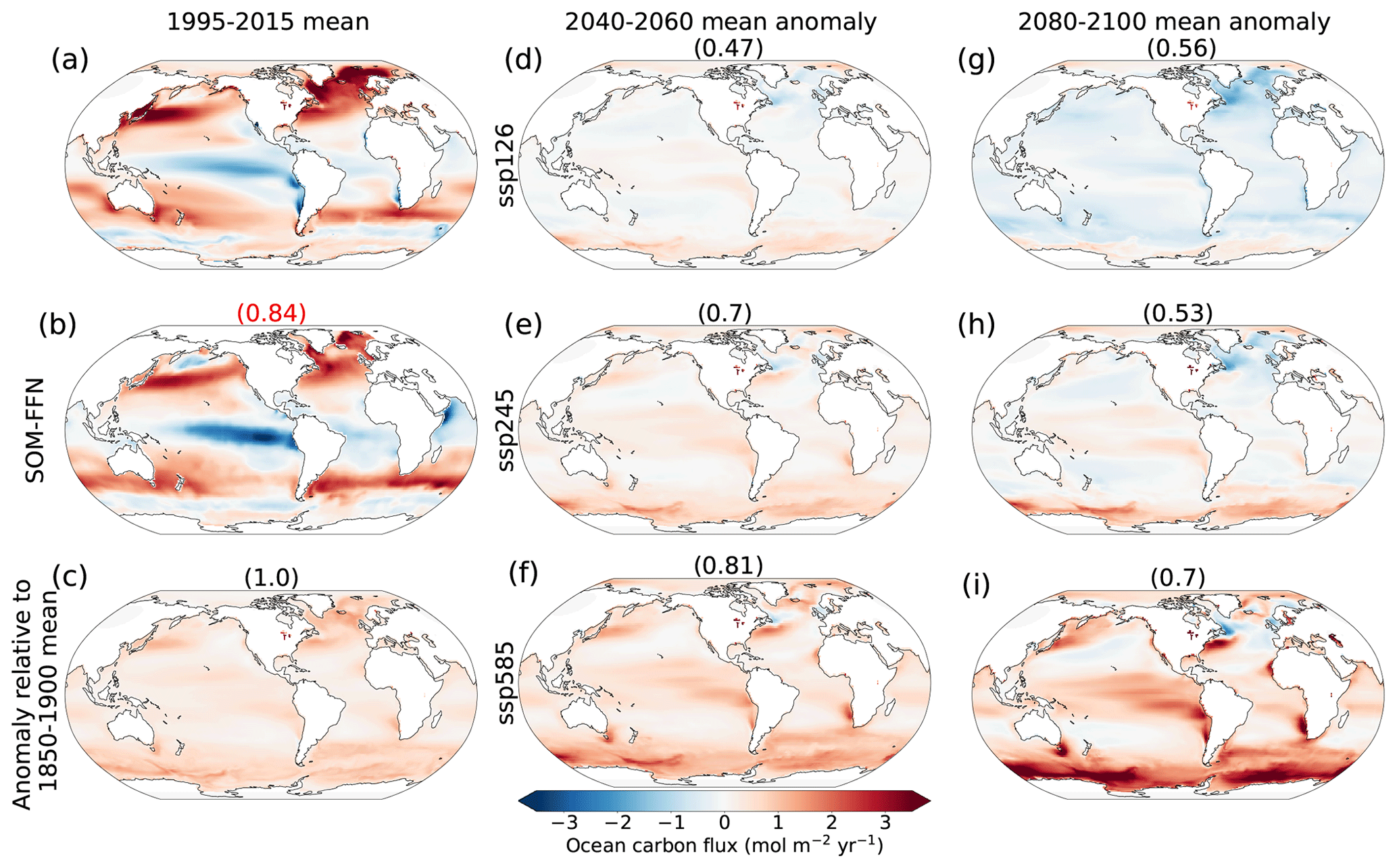
Figure 1 CMIP6 multi-model mean maps of carbon sink and sink anomalies using one realization of each model. Columns represent different time periods: the recent time (1995–2015 mean), mid-century (2040–2060 mean), and late century (2080–2100 mean). Note: the sink is positive into the ocean. The first column shows (a) the CMIP6 ensemble mean air–sea CO₂ flux over 1995–2015, (b) the Landschützer et al. (2016) SOM-FFN product, and (c) the CMIP6 ensemble mean flux anomaly over 1995–2015 relative to the 1850–1900 mean. Other panels are anomalies relative to the 1995–2015 multi-model mean (a). Panels (d) through (i) show different scenarios. Numbers above each map are correlation coefficients between the absolute value of the change relative to 1995–2015 with the 1995–2015 anomaly map relative to the pre-industrial era in (c), except the red number at the top of (b), which is the correlation coefficient with this panel and (a).

2.4 Scale dependence

Finally, the scale dependence of the sources of uncertainty is measured at year 2050 using ssp245 for internal variability and model uncertainty and using all scenarios for scenario uncertainty. The analysis is done by moving a sliding sample window of a given area across the Earth and then repeating with a larger and larger window until all scales from <100 km² to the whole Earth are considered. For each source of uncertainty and averaging scale, the average for all rectangles across the globe is reported, with each rectangle containing the same ocean area.

3 Results and discussion

3.1 Global analysis

The pattern of the carbon sink in the CMIP6 multi-model ensemble mean from the historical experiment over 1995–2015 matches that of the Landschützer (2016) self-organizing map–feed-forward neural network (SOM-FFN) observation-based data product estimate (correlation coefficient of 0.84; compare Fig. 1a, b). We use the multi-model mean response to external forcing as a more robust estimate of the forced climate signal than the response of any single model (Tebaldi and Knutti, 2007). Unlike in ESMs, the observation-based product only represents the one realization of the real world, which includes internal variability and is therefore not directly equivalent to the forced signal. However, the comparison to the 20-year mean multi-model mean still informs us about the degree of agreement between the two products. When compared to the observation-based data product, the CMIP6 multi-model mean shows a larger sink (positive flux) in the North Atlantic, North Pacific, and northwestern Pacific but a smaller sink in the Southern Ocean (Fig. 1a, b). Additionally, the observation-based data product shows a larger source in the equatorial Pacific and Indian Ocean than the CMIP6 multi-model ensemble.

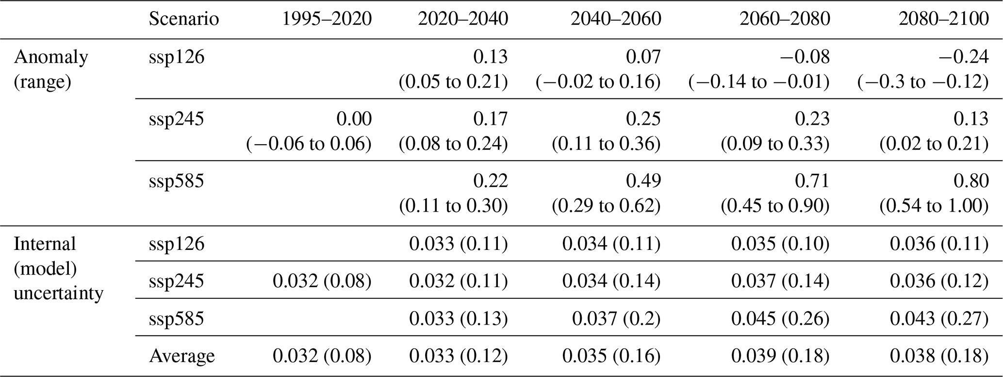
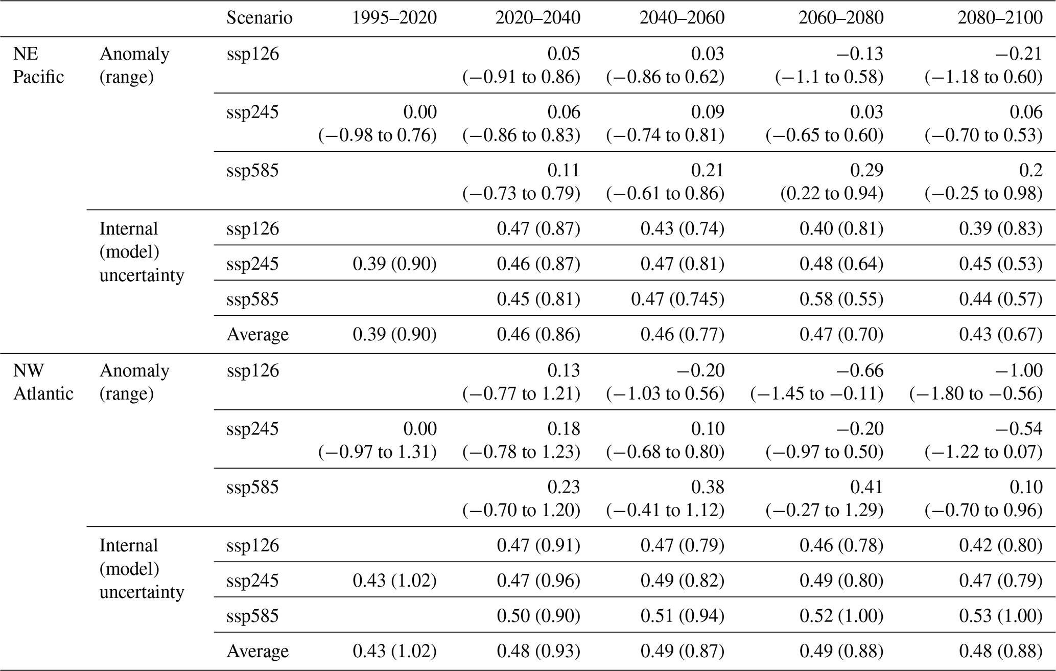
Table 1 CMIP6 multi-model mean globally averaged carbon sink anomalies (with ranges within the 20-year period in parentheses) relative to the 1995–2015 mean (in mol C m⁻² yr⁻¹) and internal variability from CanESM5 (with model uncertainty in parentheses) for the globally averaged ocean carbon sink anomalies for the three scenarios and the average values across scenarios.

While most of the global ocean shows a net sink relative to the pre-industrial era, the largest acceleration of that sink takes place in some highly active regions such as the subpolar North Atlantic, Southern Ocean, eastern equatorial Pacific, and western boundary currents of the midlatitude gyre systems in the Pacific and Atlantic Ocean (Fig. 1c). These regions of largest change in the carbon sink (direct response to higher atmospheric CO₂ plus changes in the natural carbon sink) are the regions where there is a surface–depth connectivity through ocean circulation as the air–sea flux of anthropogenic carbon is fundamentally limited by the rate of surface-to-depth transport (Graven et al., 2012; Ridge and McKinley, 2021). These results for CMIP6 models are consistent with those from McKinley et al. (2016) based on CESM-LE under CMIP5 protocols and earlier studies such as Sarmiento et al. (1998). Here, we provide a new criterion for identifying these highly active regions based on comparing the integrated global sink anomaly within grid cells above a certain threshold to the percentage of ocean area they occupy (see Sect. S5). We find that for all three scenarios and both the mid-21st century (2040–2060 mean) and late 21st century (2080–2100 mean) time periods (with the exception of ssp126 late century for which strong mitigation of anthropogenic CO₂ emissions results in broad patterns of negative anomalies), approximately 70 % of the changes in the sink relative to the pre-industrial era take place in less than 40 % of the global ocean (see Figs. S6 and S7). The diagnosed highly active regions based on this analysis (Fig. S7) are consistent with the regions of large uptake change (trends) from previous studies (Rodgers et al., 2020; McKinley et al., 2016; Frölicher et al., 2015)

The regions of the largest future carbon uptake, relative to the 1995–2015 mean, are within the same highly active regions responsible for most of the uptake over the historical period. The correlation coefficients at the top of each panel in Fig. 1 (except panel b) represent the pattern correlation between future absolute anomalies relative to 1995–2015 and anomalies in 1995–2015 relative to the pre-industrial era. The high correlations indicate that regions that have been most active in increasing their carbon sequestration are the same regions that will continue to increase further into the future, particularly with larger increases in atmospheric CO₂ (ssp585). Our results support the findings of Wang et al. (2016), who showed that projected future air–sea CO₂ fluxes are strongly associated with simulated historical air–sea CO₂ fluxes. This confirms that the historical state is a good predictor for the future state (Wang et al., 2016) not only in terms of magnitudes of the sink, but also in the spatial pattern.

The multi-model mean sink anomalies for two future periods, 2040–2060 and 2080–2100, show how the sink is projected to evolve, relative to 1995–2015, according to time and choice of emission scenario (Fig. 1d–i). The regional patterns show mostly positive anomalies at mid-century with the largest changes in the higher emission scenarios (ssp585). Towards the end of the century, however, greater areas of negative anomalies are expected in ssp126, as emissions turn negative in the late 21st century in this scenario. The largest absolute values of anomalies are still within the same highly active regions discussed before with surface–depth connectivity regardless of it being positive or negative. The late century anomalies are predominantly positive in ssp585, which corresponds to the highest emission scenario (continuing to grow larger compared to the mid-century), while ssp245 is somewhere in between, with regions of positive and negative anomalies. Under ssp245, as CO₂ emissions decrease and atmospheric CO₂ starts to level off, the intensity of uptake decreases in the midlatitude western boundary currents and subpolar North Atlantic in the late century, and anomalies in the eastern equatorial Pacific also decrease, compared to the mid-century. The globally integrated ocean carbon uptake anomaly rates are summarized in Table 1.

The trends in the global mean ocean carbon sink anomalies over 1995–2015 are statistically consistent between the CMIP6 multi-model ensemble mean and the Landschützer et al. (2016) observation-based data product (Fig. 2a) based on the test from Santer et al. (2008; see Sect. S5). However, the SOM-FFN-based time series shows a larger multi-decadal variability (variations in the 10-year running mean time series on top of the trend) than seen in individual model realizations and is larger than the range of internal variability estimated from the CanESM5 SMILE. The difference could be due to either overestimation of internal variability by the SOM-FFN method or underestimation of the internal variability by the ESMs. Given that on regional scales the SOM-FFN data are within the range of internal variability projected by the CMIP6 large ensemble of CanESM5 (see Sect. 3.3) and that there are significant gaps in the spatial and temporal sampling that underlie the Landschützer et al. (2016) estimate, it seems plausible that the discrepancy is largely due to overestimation of internal variability on the global scale by the SOM-FFN technique. This is consistent with the findings of Gloege et al. (2021), which showed that, globally, the magnitude of decadal variability is overestimated by 21 % by the SOM-FFN technique, attributed to the amount of data filling.

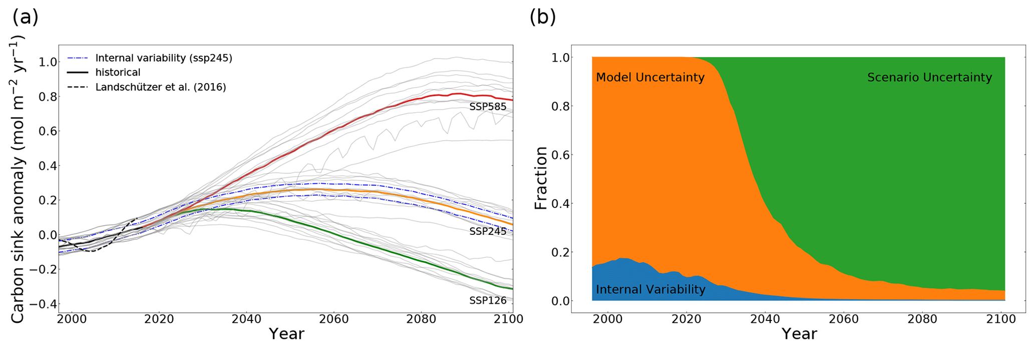
Figure 2 (a) Thick lines are multi-model means of the global mean ocean carbon sink anomaly time series relative to 1995–2015. Individual models are plotted as thin grey lines in the background. The black dashed line shows the Landschützer et al. (2016) SOM-FFN product. Both models and SOM-FFN time series are smoothed with a 10-year running mean. The blue dashed lines show internal variability for ssp245. (b) Time series showing the breakdown of uncertainty to different sources with time for the global ocean carbon sink anomaly. The internal uncertainty and model uncertainty are averaged for different scenarios.

On the global scale, model uncertainty is the dominant source of uncertainty in the historical period, but scenario uncertainty comes to dominate later (Fig. 2b). Over the 1995–2020 period, model uncertainty explains around 85 % of the total uncertainty. Scenario uncertainty becomes the dominant source after 2040, explaining almost 40 % of the total uncertainty at that time and more than 90 % by the end of the century. Internal variability explains 15 % at the start of the century but only around 1 % by the end. It is worth mentioning that the decreased share of uncertainty associated with model and internal variability does not mean that model variability or internal variability decreases in an absolute sense; rather, their importance relative to scenario uncertainty declines. These results regarding the importance of model and scenario uncertainties for multi-decadal projections and dominance of scenario uncertainty with time agree with previous studies using CMIP5 models (Lovenduski et al., 2016; Schlunegger et al., 2020).

Absolute internal and model uncertainty of the global carbon sink changes with time based on the scenario (Table 2, Fig. S3). High emission scenarios such as ssp585 show a larger change for both internal and model uncertainty where the forcing is stronger (Fig. S3). When averaged for the three scenarios, a constant increase in the magnitudes of both model variability and internal variability is seen through the century until 2080–2100 when the values either do not change or decrease slightly (Table 1). Model uncertainty more than doubles towards the end of the century compared to 1995–2015 on average for different scenarios. This is consistent with Lovenduski et al. (2016), who argue that the increase is due to differences in climate sensitivity among models that manifest more strongly with time (and hence cumulative emissions). Additionally, the dependence of internal variability on the scenario is an interesting result. Future SMILEs from multiple models will allow evaluation of the degree of dependence and the driving mechanisms of such changes with time based on the forcing (scenario). Our result of internal variability dependence on scenario implies that the time of emergence of a signal out of internal variability will be affected by changes in the internal variability under different future forcing scenarios – which we return to in Sect. 3.4.

3.2 Dependence of the sources of uncertainty on spatial scale

It is generally accepted that uncertainty and, most importantly, internal variability grow larger as the averaging (integration) scale gets finer because on larger scales the variability is averaged out. Here, we provide a novel and continuous view of change in variability across scales from the global to grid scale by measuring how variability changes relative to scale on average (Fig. 3). At the global scale, the dominant source of uncertainty is scenario uncertainty, followed by model and internal variability, respectively, consistent with Fig. 2b. However, as the averaging (integration) scale gets finer, model variability and internal variability grow rapidly, while scenario uncertainty only grows slightly on average (over all regions of this size). At an averaging (integration) scale with an area finer than 75×10⁶ km² (on average), model uncertainty becomes the dominant source of uncertainty, and at a scale finer than 3×10⁶ km², internal variability becomes larger than scenario uncertainty. The idea of scale dependence of these uncertainties was tested in Lovenduski et al. (2016) by comparing an area covering the California Current System with the global ocean. Here, we provide a novel analysis on a continuum of scales covering global to regional to local scales. While the results here hold true on average over the global ocean, scale dependence is partially controlled by the particular region being sampled. Finally, while our estimates of the magnitudes of sources of uncertainty and the crossover points (at which the dominance of internal variability over model uncertainty and model uncertainty over scenario uncertainty takes place) depend on the choice of ESMs and the method for calculation of internal variability, the general patterns are unlikely to be model-dependent.

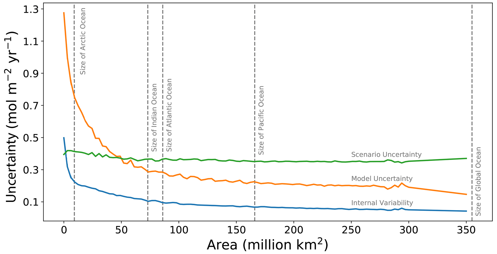
Figure 3 Sources of uncertainty versus area of averaging. Internal variability is based on ssp245 year 2050 of all CanESM5 members. Scenario uncertainty is based on all scenarios of the 13 models at year 2050, and model uncertainty is the corrected standard deviation of our 13 models at year 2050 of ssp245. The values of uncertainties are averaged over all different rectangular areas of each size that can scan the globe. Dashed lines indicate the size of the averaging window and not a specific location.

3.3 Regional analysis

We further expand on the findings of our analysis of the scale dependence of uncertainty averaged over the globe by repeating the uncertainty breakdown for two specific regions: one in the northeastern Pacific (NE Pacific) between 130–160^∘ W and 40–60^∘ N and one in the northwestern Atlantic (NW Atlantic) between 40–70^∘ W at the same latitude. We chose these regions, first, to be of similar size and second to represent very different carbon processes. The NW Atlantic region represents a highly active region, while the NE Pacific region is more typical of quiescent ocean regions, where the flux anomalies are relatively small.

The variation across scenarios is at all times smaller than internal variability in the NE Pacific (Fig. 4a). This suggests that it will be difficult to robustly detect any human-induced changes in observations of the NE Pacific carbon sink and that potential future differences relating to choice of mitigation scenarios will not be readily apparent in the NE Pacific carbon flux. This is true even for the high emission scenarios because the anomalies are small regardless of scenario (Table 2). We speculate that in the absence of mechanisms providing a pathway to the depth where significant CO₂ accumulation occurs, the surface pCO₂ trend will follow that of the atmosphere closely, causing ΔpCO₂ and therefore air–sea carbon flux to remain fairly constant for all scenarios. In the NW Atlantic, however, the variation across scenarios becomes larger than the internal variability in the early 2060s (Fig. 4c). The response of the region to climate change is dependent on the scenario (Table 2) or, in other words, the amount of carbon dioxide in the atmosphere. This is because the NW Atlantic is a highly active region where the air–sea flux actively responds to the atmospheric CO₂ concentration. The connection to depth allows surface water to be replaced with water masses whose pCO₂ trend lags behind that of the atmosphere. The trend of the CMIP6 multi-model time series over the historical period is statistically consistent (See Sect. S5) with that of the observation-based SOM-FFN product, and the multi-decadal variability is within the range of internal variability measured by the CanESM5 large ensemble in both regions. We note that both of these regions are relatively well sampled, which may lead to more robust estimates of multi-decadal variability in the Landschützer et al. (2016) dataset and better agreement with the models than seen at the global scale.

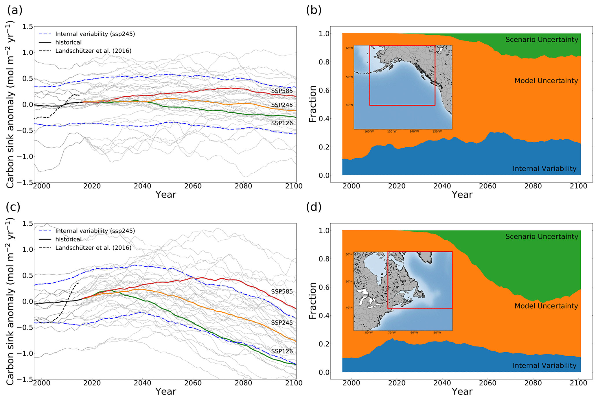
Figure 4 (a, c) Thick lines are multi-model mean time series of anomalies relative to the 1995–2015 mean. All model time series averaged for the means are plotted in grey lines in the background. The black dashed line shows the Landschützer et al. (2016) SOM-FFN product. The blue dashed line shows the internal variability measured as 2 times the standard deviation across all 50 members of the CanESM5 SMILE only for ssp245 here. (b, d) Time series showing the breakdown of uncertainty to different sources with time. The internal uncertainty and model uncertainty are averaged for different scenarios. (a, b) NE Pacific (40–60^∘ N, 130–160^∘ W). (c, d) NW Atlantic (40–60^∘ N, 40–70^∘ W).

Fractional estimates of each source of uncertainty vary with time and have different patterns for these two regions. Internal variability and model uncertainty in the NE Pacific and NW Atlantic are larger by an order of magnitude than at the global scale (Table 2). Lesser importance for scenario uncertainty and greater importance for internal and model uncertainty are apparent in both regions compared to the global scale, in agreement with Schlunegger et al. (2020). Over the period 1995–2020, model uncertainty is the dominant source of uncertainty in both the NE Pacific and NW Atlantic (80 %–90 %), while the remainder is internal variability (Fig. 4b, d). Internal variability explains around 25 %–30 % of the total uncertainty in the NE Pacific throughout the century. In the NW Atlantic, however, its share drops to 15 % by the end of the century. The share attributable to internal variability is much larger during the 21st century in both regions compared to the global scale. Internal variability is larger in the NW Atlantic in an absolute sense (Table 2), but its share of the total uncertainty is larger in the NE Pacific (Fig. 4b). The large share of internal variability in the NE Pacific indicates the need for sustained observations in the region. Overall, internal variability averaged over the scenarios shows a small increase but no clear trend in time in both regions until the 2080–2100 period when it decreases, consistent with the global estimates (Table 2). We showed earlier that in the NE Pacific scenarios do not differ because the region is not a highly active region (Fig. S7) – scenario uncertainty explains less than 20 % of the total uncertainty at the end of the century in the NE Pacific. In the NW Atlantic, scenario uncertainty grows larger with time, becoming 45 %–50 % of total uncertainty by the end of the century. In both regions, model uncertainty is the dominant source of uncertainty in all years.

Our regional analysis confirms that while uncertainty and its distribution among sources depend on the spatial scale of integration, the specific location also matters (Lovenduski et al., 2016; Schlunegger et al., 2020). Schlunegger et al. (2020) tested this idea for 10 ocean basins of variable size (see their Fig. 9). We focused on keeping the sizes similar and analyze a highly active region versus a more quiescent ocean region. The key message here that there is an association with the importance as well as the magnitude of sources of uncertainty with how active the region is in regards to the carbon sink is not sensitive to the use of CanESM5 for estimation of internal variability. Local patterns of uncertainty broken down by source are thus needed to clarify changes based on location.

Table 2 CMIP6 multi-model mean sink anomalies (with ranges in parentheses) relative to 1995–2015 mean (in mol C m⁻² yr⁻¹) and internal variability (with model uncertainty in parentheses) for the three scenarios and their average values in NE Pacific and NW Atlantic.

Consistent with the sink anomaly maps (Fig. 1), the regions that show the highest uncertainty for any of the sources in the future are the same regions that show the largest uncertainties in the historical period (Fig. 5). More importantly, the regions of the largest future uptake uncertainty are highly correlated with the historical regions of largest uptake (relative to the pre-industrial ocean), as shown by the pattern correlation coefficients above each panel. This is an important finding, because it suggests that knowledge of the regions of modern-day surface carbon flux anomaly provides us with information about regions of future uptake uncertainty.

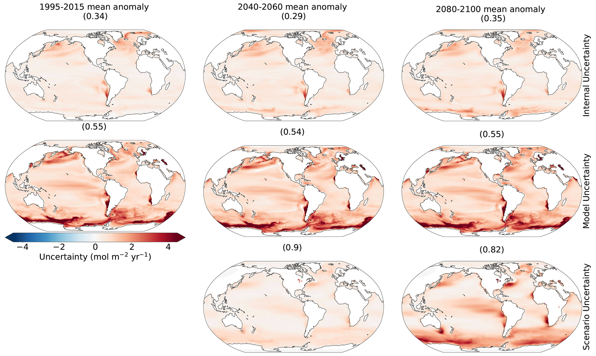
Figure 5 Sources of uncertainty averaged over the 20-year mean periods. The rows represent different sources as explained in the “Data and methods” section at each grid cell. Columns represent different times: the recent (1995–2015), mid-century (2040–2060), and late century (2080–2100) anomalies relative to the 1995–2015 mean. The numbers are correlation coefficients of each map with the 1995–2015 mean anomaly relative to the 1850–1900 mean (Fig. 1c).

Internal variability from CanESM5 is most dominant in midlatitude eastern boundary upwelling regions and their extensions, in the North Atlantic, in the western boundary currents of the Gulf Stream and Kuroshio and their extensions, and in the Southern Ocean (Fig. 5). There is wide agreement between different models and estimation methods on regions of the largest internal variability (Fig. S4). The regions of large internal variability are correlated with the same highly active regions for the sink anomalies discussed earlier (Fig. 1c). This is consistent with McKinley et al. (2017), who argue that modeling and observational studies show that the primary drivers of variability in the ocean carbon uptake are ocean circulation and ventilation of the deep ocean. However, correlation coefficients between internal variability and historical uptake are lower than those seen for scenario and model uncertainty. An increase in internal variability with time is seen mostly in the Southern Ocean, the Arctic Ocean, and boundaries of the gyre systems, while the rest of the ocean does not show a clear change. The maps in Fig. 5 are averaged over the three scenarios, which masks the changes to some extent. However, we show in the Supplement (see Sect. S2) that changes in the globally averaged internal variability with time are different for different scenarios.

Model uncertainty is consistently highest in the highly active regions (Fig. S7), leading to strong correlation with the anomaly maps of Fig. 1c. In these regions, ocean circulation impacts surface pCO₂ through advection and water mass transformation regionally (Bopp et al., 2015; Toyama et al., 2017), and models have substantial differences in ocean circulation. Ridge and McKinley (2021) suggest that while global surface carbon fluxes and carbon storage are largely similar across ESMs over the historical period, consistent with the external forcing from atmospheric pCO₂ growth being the main driver of the historical sink (McKinley et al., 2020), uncertainties in ocean circulation may become important in the future under a changing trajectory of atmospheric boundary conditions. The model uncertainty is largest in the Southern Ocean, consistent with CMIP5 models (Frölicher et al., 2015). Here, mode and intermediate waters are formed, and the complex nature of processes governing the sinks varies on all timescales (Gruber et al. 2019). Frölicher et al. (2015) note the largest disagreement in ocean carbon uptake between models is in the Southern Ocean because the exact processes governing heat and carbon uptake remain poorly understood. The importance of model uncertainty in the Southern Ocean provides a clear focal point for modeling centers to concentrate their efforts in reducing projection uncertainty.

Scenario uncertainty exhibits the largest change with time. This is by construction as the scenarios deviate from each other with time to represent a range of pathways for future socioeconomic possibilities in order to assess the long-term impacts of short-term decisions (Riahi et al., 2017). Importantly, the correlation coefficients are highest between scenario uncertainty and the current regions of large sink anomaly, indicating that the same highly active regions are the regions that show the largest divergence among scenarios and that the sink in most other regions does not respond as strongly to scenario differences. We showed an example of this earlier (Fig. 4), where the time series of the multi-model signals for the three scenarios did not emerge out of internal variability in the NE Pacific by 2100, whereas they did for the highly active region of the NW Atlantic. This shows that with pCO₂ differences across the air–sea interface being the main driver of the sink (Fay and McKinley, 2013; Landschützer et al., 2015; Lovenduski et al., 2007; McKinley et al., 2017, 2020), the sink in these active regions evolves as the atmospheric CO₂ concentration changes because ocean processes associated with surface–depth connectivity constantly dampen the surface ocean pCO₂ trend compared with that of the atmosphere. In other words, the surface water in these regions is constantly renewed, mostly through advection and water mass formation, with water masses whose pCO₂ has not increased at the same rate as the atmosphere. Elsewhere, these conditions do not hold true and surface water trends match that of the atmosphere, decreasing the sensitivity of the sink anomaly to the projection scenario. These uncertainties are central to the ability to detect human-induced trends in observations of the surface ocean carbon flux as well as to assess mitigations or make societal decisions, to which we now turn.

3.4 Detectability

Detectability refers to the ability to robustly identify a forced signal, above and beyond the noise induced by internal climate variability. Previous studies have largely presented a single time of emergence (Lovenduski et al., 2016; Schlunegger et al., 2019; McKinley et al., 2016). However, understanding the regional differences, timescales, and scenario dependence in the detectability of human-induced trends in the ocean surface carbon flux is important for informing observational strategies that aim to measure these changes.

We measure the detectability of the CMIP6 multi-model ensemble mean ocean surface carbon flux anomaly using the time of emergence at each grid point. We use this finest scale as it is the most applicable to observational communities for sampling. The time of emergence is defined as the point at which the forced signal, given by the multi-model ensemble mean flux anomaly, relative to 1995–2015, emerges from internal variability, given by the CanESM5 SMILE.

The signal in human-induced surface ocean carbon flux emerges beyond the internal variability earlier in the highly active regions than anywhere else. This is evident in the equatorial Pacific, Southern Ocean, the western boundary currents of the gyre systems, and their extensions (Fig. 6). Ocean regions such as the centers of the midlatitude gyre systems and the NE Pacific show late emergence times and, in some cases, no detectability of the signal in any of the scenarios by 2100. Convergent large-scale circulation and strong stratification in these regions isolate the surface from the deep ocean, limiting their capacity to accelerate their uptake of anthropogenic carbon (McKinley et al., 2016). An absence of mechanisms constantly drawing surface ocean CO₂ trends out of equilibrium with atmospheric CO₂ lets the surface water adjust to the atmospheric trend on short timescales. Significant changes thus do not take place in the sink as the atmospheric CO₂ levels change and scenario uncertainty is lowest in the same regions (see Fig. 4). This is consistent with the results from Sect. 3.3, in which we showed that internal variability is a significant source of uncertainty throughout the century in the NE Pacific, with scenarios never emerging out of the range of internal variability (Fig. 4a, b). Our results for the broad patterns in the multi-model mean TOE are largely consistent with previous studies, suggesting they are robust and insensitive to the method of estimating internal variability. These include studies with single-model large ensembles such as McKinley et al. (2016) that assumed time- and scenario-independent internal variability and CMIP5 models such as Schlunegger et al. (2020) that used only high-emission-scenario internal variability from four large ensembles to show there is strong agreement between the TOEs of the large ensembles (LEs) both locally and spatially. Our results argue that observational records inside highly active regions are likely sufficient to detect human influence on the ocean carbon sink in the coming years and decades (2030–2050) if not earlier. Meanwhile, they imply that observational time series in quiescent regions, such as Ocean Station Papa in the NE Pacific, need to interpret any observed trends with care, since internal variability tends to dominate over human-induced trends.

Figure 6 Time of emergence of the multi-model mean anomaly under different scenarios. White regions indicate where the anthropogenic signal cannot be detected even towards the end of the century.

Time of emergence strongly depends on the future scenario. Schlunegger et al. (2020) show for two scenarios that modest (∼10-year) TOE differences between different ESMs under strong anthropogenic forcing can evolve into pronounced (60 +-year) TOE differences with moderate mitigation. Here, we make use of three scenarios including a strong mitigation scenario and account for scenario dependence of internal variability in our approximation using CanESM5. On average, scenarios with smaller forced trends emerge later as the size of the forced trend is critical to the time of emergence (Fig. 2a). The TOE is earliest on average over the global ocean in ssp585, while it is later in ssp245 and later still in ssp126, consistent with the imposed changes in atmospheric CO₂ concentration. The exceptions are quiescent regions that show earlier detectability for ssp126 compared to other scenarios; these exceptions are associated with larger (but negative) anomalies in the latter half of the century under ssp126, which has negative emissions (compare panels d–f and g–i in Fig. 1). Internal variability does evolve somewhat differently for each scenario, but this is secondary (Fig. S2). Schlunegger et al. (2020) argue that variables such as air–sea CO₂ flux, which are sufficiently sensitive to emissions, emerge early, prior to significant divergence among future scenarios. Consistent with this result, our results indicate that there is broad agreement between scenarios in the TOE patterns when considering the highly active regions. Interestingly, our scenario-specific TOE shows that differences between scenario TOEs are associated with how sensitive different regions are to emission scenarios. More specifically, comparison to the maps of scenario uncertainty (Fig. 5) shows that TOE differs more across scenarios in regions where scenario uncertainty is small, such as the aforementioned subtropical Ekman convergence regions. Elsewhere, the emergence happens before scenarios diverge significantly. Our results suggest that under the rapidly rising atmospheric CO₂ concentrations seen in ssp585, the human signal in the ocean carbon sink will likely be detectable across much of the global ocean over the coming few decades. However, under strong mitigation scenarios, such as ssp126, early emergence (e.g., earlier than 2030) is not expected to occur except in isolated regions, while counterintuitively, a lower percentage of the global ocean area remains non-emergent by 2100.

4 Conclusions

Ocean uptake of the increasing atmospheric CO₂ in the 21st century is concentrated in a few active regions with 70 % of the total changes in the sink occurring in less than 40 % of the global ocean. We analyze the results from the CMIP6 multi-model mean for the current state of the ocean (1995–2015) and the middle (2040–2060) and late (2080–2100) 21st century relative to the current state for three scenarios. We show that future changes in the sink are projected to mostly take place within the same historically highly active regions, including the North Atlantic and Southern Ocean. Our results extend the argument of Wang et al. (2016) that the historical state is a good predictor of the future state to spatial patterns of change.

We show that the CMIP6 multi-model mean provides a consistent estimate of the spatial patterns of the sink and the trend in the sink (globally) compared to the observation-based data product of Landschützer et al. (2016). These results suggest the CMIP6 models are valid tools for understanding the past and future evolution of the ocean carbon sink, particularly at broad spatial scales. A notable area of disagreement is that the Landschützer et al. (2016) data show larger decadal variability at the global scale than seen in any CMIP6 model or the range of internal variability from the CanESM5 large ensemble. Gloege et al. (2021) show that the SOM-FFN method overestimates the magnitude of decadal variability on the global scale due to the amount of gap filling.

We have shown that the magnitude of uncertainty and its partitioning among different sources differ with scale and location. On the global scale, scenario uncertainty is the largest source of uncertainty, followed by model uncertainty and internal variability for CMIP6 models. These results are in agreement with previous studies from the CMIP5 models (Lovenduski et al., 2016; Schlunegger et al., 2020). As the scales of integration (averaging) get finer, model variability and internal variability become the dominant sources, respectively. Testing the results on two ocean regions of about the same size, one in the NE Pacific and one in the NW Atlantic, shows that – while consistent with the results of the scale dependence analysis – the relative importance of the sources of uncertainty also differs with location. Our test here extends the analysis Schlunegger et al. (2020) with a focus on the association of the location dependence with whether the regions have highly active carbon sinks. Notably, in highly active regions, such as the NW Atlantic, scenario uncertainty is large, whereas in more quiescent regions, such as the NE Pacific, internal variability is more important. The time and scenario dependence of internal is another interesting finding that could be the subject of future studies to achieve a better understanding of the driving mechanism and the degree of dependence on future emissions and/or concentrations.

The patterns of high future CO₂ uptake uncertainty are highly correlated with the patterns of historical uptake. The correlation coefficients are highest for scenario uncertainty, indicating that the highly active regions have the potential for the sink to evolve according to the atmospheric CO₂ concentration, while the rest of the ocean basins do not respond strongly to changes in atmospheric CO₂ represented by the different scenarios. This finding has implications for assessment of mitigation and effects of socioeconomic decisions. Our results here are significant in that they show that regions of future uncertainty are strongly associated with known regions of large historical uptake.

Patterns seen in the time of emergence have implications for observational campaigns for detection of a signal (Schlunegger et al., 2019, 2020). There is a reverse association between how sensitive a region is to scenario differences (apparent in the scenario uncertainty patterns) and how sensitive the TOE is to scenarios. Our results show that caution should be taken in interpreting the observed changes in regions such as the NE Pacific associated with late emergence of the signal from the decadal (internal) variability. On the other hand, consistent observations in regions such as the equatorial Pacific, the Gulf Stream and Kuroshio and their extensions, and the Southern Ocean are likely to detect the emergence of the forced signal out of internal variability earlier in time. Additionally, the patterns in sources of uncertainty show that model uncertainty is largest in the Southern Ocean, consistent with Frölicher et al. (2015). The sink in the Southern Ocean is driven by complex mechanisms involving coupled ocean–atmosphere–ice interactions that require better representation in ocean biogeochemical models. Significant progress in reducing uncertainties can be expected from new methods of bringing together models and observations (Frölicher et al., 2016). Our results provide a motivation to focus modeling as well as observational efforts on the known highly active regions of historical uptake.

Finally, we have shown that internal variability shows clear changes in time and depends on the scenario. The emergence of large ensembles (LEs) allows for quantification of these variations if enough ensemble members are available to fully capture internal variability using realizations that start from different initial conditions. Our use of the CanESM5 LE allows us to account for the nonstationary of internal variability in time, like in Schlunegger et al. (2020), but with the advantage of also accounting for scenario dependence. Model intercomparison indicates that ESMs show differences in natural variability (Schlunegger et al., 2020). Nonetheless, our analyses of the global scale, of scale dependence, and of the patterns seen in time of emergence are consistent with previous studies, despite the potential sensitivity to the use of CanESM5 LE. Our methodology to correct for internal variability from model spread, without filtering or having a large ensemble for each ESM (which would limit the number of ESMs that can be included and, consequently, underestimate model uncertainty), lays the foundation for future studies when LEs are available from more ESMs and suggests a need for more modeling groups to provide such LEs in order to achieve a more robust estimate of internal variability across different ESMs.