Seasonal forecasting skill for the High Mountain Asia region in the Goddard Earth Observing System

Seasonal variability of the global hydrologic cycle directly impacts human activities, including hazard assessment and mitigation, agricultural decisions, and water resources management. This is particularly true across the High Mountain Asia (HMA) region, where availability of water resources can change depending on local seasonality of the hydrologic cycle. Forecasting the atmospheric states and surface conditions, including hydrometeorologically relevant variables, at subseasonal-to-seasonal (S2S) lead times of weeks to months is an area of active research and development. NASA's Goddard Earth Observing System (GEOS) S2S prediction system has been developed with this research goal in mind. Here, we benchmark the forecast skill of GEOS-S2S (version 2) hydrometeorological forecasts at 1–3-month lead times in the HMA region, including a portion of the Indian subcontinent, during the retrospective forecast period, 1981–2016. To assess forecast skill, we evaluate 2 m air temperature, total precipitation, fractional snow cover, snow water equivalent, surface soil moisture, and terrestrial water storage forecasts against the Modern-Era Retrospective analysis for Research and Applications, Version 2 (MERRA-2) and independent reanalysis data, satellite observations, and data fusion products. Anomaly correlation is highest when the forecasts are evaluated against MERRA-2 and particularly in variables with long memory in the climate system, likely due to the similar initial conditions and model architecture used in GEOS-S2S and MERRA-2. When compared to MERRA-2, results for the 1-month forecast skill range from an anomaly correlation of R_anom=0.18 for precipitation to R_anom=0.62 for soil moisture. Anomaly correlations are consistently lower when forecasts are evaluated against independent observations; results for the 1-month forecast skill range from R_anom=0.13 for snow water equivalent to R_anom=0.24 for fractional snow cover. We find that, generally, hydrometeorological forecast skill is dependent on the forecast lead time, the memory of the variable within the physical system, and the validation dataset used. Overall, these results benchmark the GEOS-S2S system's ability to forecast HMA hydrometeorology.

1 Introduction

Skillful prediction of hydrometeorological conditions at subseasonal-to-seasonal (S2S) timescales depends on a range of factors, including the representation of land and ocean initial conditions (Dirmeyer et al., 2018; Mariotti et al., 2018), a model's ability to capture large-scale atmospheric processes (Gibson et al., 2020), a model's representation of climate mode variability (e.g., Waliser et al., 2006, 2009; Shukla et al., 2018), the chosen perturbation and ensemble scheme (Scaife et al., 2014), and the level of predictability itself. S2S forecasting differs from numerical weather prediction, where skill largely depends on accurate representation of atmospheric initial conditions (Pielke Sr. et al., 1999). There is a need to understand the processes that drive S2S prediction skill, and there has been extensive research (e.g., Merryfield et al., 2020; White et al., 2021) aimed towards understanding the complexity of these systems. However, further improvements in S2S forecasting skill, particularly of societally relevant variables, are sought because accurate S2S forecasts are useful for advance planning in various sectors, such as energy, water resources, agriculture, and disaster mitigation (National Academies Press, 2016).

S2S hydrometeorological forecasts can be valuable in heavily populated regions, such as the Indian subcontinent, as well as in more sparsely populated areas, such as High Mountain Asia (HMA). These regions experience substantial inter- and intra-annual variability in water resources. HMA has been dubbed one of the main “water towers” of the Earth (Viviroli et al., 2007; Immerzeel et al., 2010, 2020) and has been hypothesized to influence global weather patterns through its impact on teleconnections (Nash et al., 2021). S2S forecasting systems, such as the Goddard Earth Observing System S2S prediction system (GEOS-S2S), could skillfully capture large-scale atmospheric patterns and teleconnections (Gibson et al., 2020; Lim et al., 2021), including those impacting the HMA region. Ding and Wang (2007) and Lim (2015) demonstrated the importance of the Eurasian teleconnection in driving the planetary-scale Rossby-wave propagation that causes the intraseasonal variability over central Asia and the northern part of India. Other studies investigated climate variations over HMA by the impact of the North Atlantic Oscillation (Li et al., 2005, 2008), the Indian Ocean Dipole and El Niño–Southern Oscillation (Stuecker et al., 2017; Sang et al., 2019; Power et al., 2021; Meena et al., 2022), the Central Indian Ocean mode (Zhou et al., 2017), and the boreal summer intraseasonal oscillation (Jiang et al., 2004; Hatsuzuka and Fujinami, 2017).

The proper representation of large-scale teleconnections in S2S forecasting systems and how that impacts hydrometeorological conditions is complicated by local characteristics, which degrade the accuracy of high-resolution S2S forecasts at local scales. For example, the northward propagation of the boreal summer intraseasonal oscillation originates in the northern Indian Ocean and tends to dissipate near the foothills of the Himalayas, and high humidity along the southern slope of the Himalayas and Tibetan Plateau leads to enhanced precipitation events (Jiang et al., 2004; Hatsuzuka and Fujinami, 2017). It is, however, extremely difficult to pinpoint specific locations where this process ultimately occurs. Therefore, to gain a better understanding and to make better predictions of how the Earth system behaves at regional scales, such as for the HMA region, further research is warranted.

Numerous investigations have examined the impacts of climate and weather in the HMA region, including air temperature (Su et al., 2013; Dars et al., 2020), precipitation (Su et al., 2013; Ghatak et al., 2018; Liu and Margulis 2019; Christensen et al., 2019; Dars et al., 2020; Stanley et al., 2020), terrestrial water storage and the overall water budget (Loomis et al., 2019a; Yoon et al., 2019), groundwater storage (Xiang et al., 2016; Wang et al., 2021), snow (Liu et al., 2021a; Liu and Margulis, 2019; Margulis et al., 2019), glaciers (Shugar et al., 2020; Maurer et al., 2020; Batbaatar et al., 2021), atmospheric river storms (Nash et al., 2021), hydropower (Mishra et al., 2020), and landslides (Bekaert et al., 2020; Stanley et al., 2020). There are many communities of scientists in the US, Europe, and Asia investigating how climate is changing in HMA and what drives these changes (e.g., Arendt et al., 2017).

More broadly, studies such as those by Vitart and Robertson (2018), de Andrade et al. (2019), and Robertson et al. (2020) have investigated the usefulness of S2S forecasting for global climate and weather extremes. These types of studies can be used to deduce the skill of S2S forecasts for the HMA region. For instance, these studies show how forecasting a variable like precipitation in the HMA region can be difficult, with forecasts being acceptable out to week 1 but starting to degrade for forecasts in weeks 2–4. Furthermore, there have been studies that investigate the skill of S2S forecasts specifically for regions including or close to HMA. For example, Deorias et al. (2021) compared the prediction of the Indian monsoon in different S2S models; Hsu et al. (2021) investigated simulations of the East Asian winter monsoon on S2S time scales; Gerlitz et al. (2020) applied climate-informed seasonal forecasts of water availability in Central Asia; and Zhou et al. (2021) developed a hydrological monitoring system and S2S forecasting system for South and Southeast Asian river basins. Many of these studies utilized S2S prediction systems, but there is still a need for further evaluation of S2S forecast skill for hydrometeorological variables in the HMA region. Our study examines the skill of S2S forecasting for the HMA region using the GEOS-S2S forecasting system.

The NASA Global Modeling and Assimilation Office utilizes the GEOS-S2S forecasting system, which initializes S2S forecasts each month using a weakly coupled atmosphere–ocean data assimilation system (Borovikov et al., 2018; Molod et al., 2020). Forecasts are provided to national and international multi-model prediction efforts, including the North American Multi-Model Ensemble (Kirtman et al., 2014). The skill of GEOS-S2S has been reported in various works, such as by Gibson et al. (2020), who assessed the hindcast skill of representing ridging events over the western United States in different S2S models and found the forecast horizon of GEOS-S2S to be comparable with other S2S models in the community. Recent GEOS-S2S system developments improved the representation of ocean temperatures and heat transport (Molod et al., 2020) and the retrospective forecast of climate indices, including the El Niño–Southern Oscillation, North Atlantic Oscillation, and the Madden–Julian Oscillation, particularly at 1–3-month lead times (Molod et al., 2020; Lim et al., 2021). These improvements should contribute to enhancements in global hydrometeorological forecast skill in GEOS-S2S.

In this study, we examine the ability of GEOS-S2S forecasts to accurately predict near-surface air temperature, total precipitation, fractional snow cover area, snow water equivalent, surface soil moisture, and terrestrial water storage across the HMA region and a large portion of the Indian subcontinent at 1-, 2-, and 3-month lead times. These variables are directly relevant to the accurate prediction of water resources and processes critical to local populations. Evaluation and improvement of hydrometeorological forecast lead time can improve warning systems for natural hazards such as flooding or landslides and can provide critical information for agricultural purposes (Bekaert et al., 2020; Stanley et al., 2020). However, the complex relationships among variables and the regional topography within HMA make S2S forecasting for this area challenging. Some of these variables, such as temperature or precipitation, are more difficult to accurately forecast at the S2S time scales compared to other variables because of their fast nature and low memory in the physical system. It is hypothesized that there is higher forecast skill for the variables with longer temporal memory in the physical system, such as snow, soil moisture, or terrestrial water storage. Therefore, proper initialization of these variables can allow for longer-lasting skill in the S2S forecasting system.

The first objective of this work is to provide a benchmark of GEOS-S2S hydrometeorological forecast skill for the HMA region and across a large portion of the Indian Subcontinent. A second objective of the analysis is to determine potential areas of improvement in model initialization or more realistic representation in the model architecture, which can help enhance the forecast accuracy in future GEOS-S2S versions and extend the skillful forecast window of variables in the HMA region. The paper is organized as follows: Sect. 2 introduces the datasets and methods used in this study, Sect. 3 reports the results of the evaluation, Sect. 4 offers a discussion on the main findings, and Sect. 5 concludes with a summary of the paper.

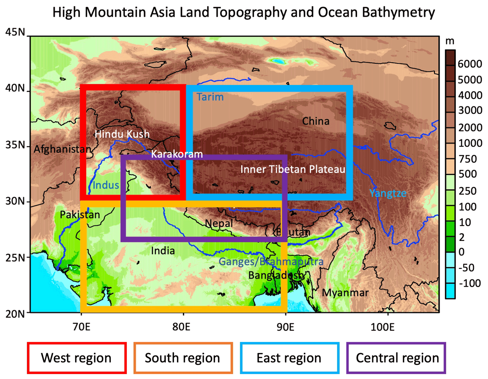
Figure 1 Topography and ocean bathymetry using the NOAA National Geophysical Data Center's ETOPO1 global relief model. The map shows the elevation (m) for the HMA domain. The topography shown in this map is not the same as the topography used by GEOS-S2S, which has a coarser representation of the actual topography in the HMA region. In this figure, countries are in black text, mountain ranges are in white text, and main rivers that are in major basins are in blue text. Four subregions are defined for additional analysis, where the west region shown in red includes the Hindu Kush and Karakoram mountains, the south region includes the Indian subcontinent, the east region includes the Inner Tibetan Plateau, and the central region includes the Himalayas.

2 Data and methods

2.1 Region of focus

Here, we refer to “HMA” as the domain shown in Fig. 1, covering parts of China, Afghanistan, Pakistan, Nepal, Bhutan, India, Bangladesh, Myanmar, Kazakhstan, Uzbekistan, Kyrgyzstan, and Tajikistan and stretching across several mountain ranges, including the Himalayas, Inner Tibetan Plateau, Karakoram, and Hindu Kush. These mountains funnel fresh water into major river basins, including the Tarim, Indus, Yangtze, and Ganges–Brahmaputra basins, that support about 1.5 billion people, providing drinking water, irrigation, and hydropower (Immerzeel et al., 2020). HMA has one of the highest concentrations of snow and glacier ice outside of the polar regions, making it an extremely important region to study and evaluate S2S forecasting of hydrometeorological variables. The HMA region we consider here includes areas of different topography, population density, and climate. For this reason, we split our domain into different subregions (shown in the boxes in Fig. 1) that account for the different areas within HMA.

2.2 GEOS-S2S prediction system

We evaluate GEOS-S2S, version 2 (Molod et al., 2020); the GEOS-S2S forecasting system is an atmosphere–ocean general circulation model (AOGCM) and ocean data assimilation system. The AOGCM includes the GEOS atmospheric general circulation model (AGCM; Molod et al., 2015; Rienecker et al., 2008), the catchment land surface model (Koster et al., 2000), version 5 of the Modular Ocean Model developed by the Geophysical Fluid Dynamics Laboratory (Griffies, 2012), and version 4.1 of the sea ice model developed by the Los Alamos National Laboratory (Hunke and Lipscomb, 2008). GEOS-S2S forecasts are initialized using a precomputed atmospheric analysis and ocean data assimilation (Penny et al., 2013). The system components are coupled using the Earth System Modeling Framework (Hill et al., 2004) and the Modeling Analysis and Prediction Layer interface layer (Suarez et al., 2007).

The GEOS-S2S analysis uses a weakly coupled atmosphere–ocean data assimilation system with a 5 d assimilation cycle. During the initial 5 d predictor segment, every 6 h, the departure of model trajectory from observed ocean fields is determined, and sea ice fraction is replaced with satellite-derived observations (Cavalieri et al., 1996). Following the predictor segment, the model is rewound, and ocean analysis increments are applied during the first 18 h of the 5 d corrector segment. During both segments, the atmosphere is nudged to a precomputed state, and SST is strongly relaxed to MERRA-2 values to ensure that the ocean and atmosphere are as consistent as possible. A detailed description is in Molod et al. (2020).

Forecasts are initialized from the GEOS-S2S analysis at the end of the corrector segment. During the retrospective forecast period (1981–2016), forecasts are initialized using an unperturbed lagged scheme, with unperturbed forecasts initialized every 5 d during the last half of each month for a total of four ensemble members. During the operational forecast period (2017–present), an additional six perturbed forecasts are initialized on the last forecast day of each month. All forecasts are 9 months in duration, but we focus here on the four ensemble members in the retrospective forecasts with 1-, 2-, and 3-month lead times. Retrospective forecasts, which are used in this study, are completed to provide a model climatology for use in probabilistic forecasting and to provide a long period for forecast verification (Molod et al., 2020). GEOS-S2S forecasts have been used and evaluated in studies related to the Madden–Julian Oscillation (Lim et al., 2021), sea surface salinity and its impact on the El Niño–Southern Oscillation (Hackert et al., 2020), the impact of volcano eruptions on surface temperatures and precipitation (Aquila et al., 2021), and others.

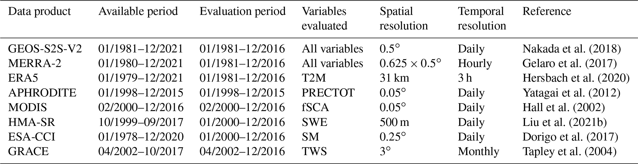
The hydrometeorological variables of interest were obtained from the GEOS-S2S archive and include the following: 2 m air temperature (T2M from the “surf” collection), total precipitation (PRECTOT from the “vis2d” collection), snow cover area fraction (ASNOW from the “vis2d” collection and called fSCA for the remainder of this paper), snow water equivalent (SNOMAS from the “vis2d” collection and called SWE for the remainder of this paper), soil moisture in the surface layer from 0–5 cm (WET1 from the “vis2d” collection and SM for the remainder of this paper), and terrestrial water storage (TWLAND from the “surf” collection and “TWS” for the remainder of this paper). The PRECTOT variable investigated here is total precipitation including rain and snowfall, i.e., PRECTOT = liquid + solid (total) precipitation. SM is calculated at each grid cell by scaling the WET1 variable with porosity. For grid cells that are frozen or are covered in snow, the soil moisture value is masked out as a no-data-value grid cell to focus on the warm season, following the work of De Lannoy and Reichle (2016). Simulated TWS includes soil moisture, snow, and the canopy interception reservoir, but not surface water (that is, lake and river water) or glaciers. Table 1 provides a list of these variables, as represented in GEOS-S2S (Nakada et al., 2018), and the corresponding evaluation datasets, detailed in the following subsections.

Table 1 The list of all data products used, including the GEOS-S2S V2 forecasting system, the MERRA-2 reanalysis product, and the various reference data products. The information in this table includes the period of data availability, the period used in the evaluation, the variables used in this study, the original spatial and temporal resolutions, and the main reference for each dataset. GEOS-S2S-V2, MERRA-2, and ERA5 data are provided up until the present day, and production of these datasets occurs in near-real-time, where quality-assured monthly updates are typically published within 3 months of data production. GRACE data are originally provided at 3^∘ spatial resolution, but the version used here is posted at 1^∘ spatial resolution.

2.3 Evaluation datasets

The first product used here to evaluate the GEOS-S2S forecasts is the Modern-Era Retrospective analysis for Research and Applications, version 2 (MERRA-2; Sect. 2.3.1; Gelaro et al., 2017). MERRA-2 and GEOS-S2S output includes many compatible variables because the version of the GEOS AGCM in GEOS-S2S-2 is similar to the version used for the production of the MERRA-2 reanalysis.

To further evaluate GEOS-S2S, we also use independent reanalysis and observational products (Table 1). To this end, for air temperature we use the fifth-generation atmospheric reanalysis from the European Centre for Medium-Range Weather Forecasts (ECMWF) reanalysis product (ERA5; Sect. 2.3.2; Hersbach et al., 2020). For precipitation, we use the Asian Precipitation – Highly Resolved Observed Data Integration Towards Evaluation product (APHRODITE; Sect. 2.3.3; Yatagai et al., 2012). For snow cover, we use the Moderate-Resolution Imaging Spectroradiometer (MODIS; Sect. 2.3.4; Hall et al., 2002) remotely sensed product. For SWE, we use the HMA Snow Reanalysis product (HMA-SR; Sect. 2.3.5; Margulis et al., 2019; Liu et al., 2021b). For soil moisture, we use the European Space Agency's Climate Change Initiative data (ESA-CCI; Sect. 2.3.6; Dorigo et al., 2017). Lastly, for TWS, we use data from the NASA Gravity Recovery and Climate Experiment satellite mission (GRACE; Sect. 2.3.7; Tapley et al., 2004). We utilize information from different sources to make sure that evaluation results are not solely dependent on biases or uncertainties in a single reference product. The datasets used for evaluation in our study have their own biases and issues, particularly over the mountainous regions of our study.

2.3.1 MERRA-2

MERRA-2 is the most recent NASA global atmospheric reanalysis product and is generated using the GEOS atmospheric model and analysis (Gelaro et al., 2017). MERRA-2 output contains similar variables to GEOS-S2S and offers a rich product to apply systematic evaluation of the model forecasts. We obtain information from MERRA-2 on all the variables of interest listed in the previous section (Table 1) and for the same period (1981–2016; Bosilovich et al., 2016). The variables of interest include the following: 2 m air temperature (T2M from the “single-level diagnostics” collection; GMAO, 2015a), total precipitation (PRECTOTCORR from the “surface flux diagnostics” collection; GMAO, 2015b), snow cover area fraction (FRSNO from the “land surface diagnostics” collection and called fSCA for the remainder of this paper; GMAO, 2015c), snow water equivalent (SNOMAS from the “land surface diagnostics” collection and SWE for the remainder of this paper), soil moisture in the surface layer from 0–5 cm (GWETTOP from the “land surface diagnostics” collection and SM for the remainder of this paper), and terrestrial water storage (TWLAND from the “land surface diagnostics” collection and TWS for the remainder of this paper). MERRA-2 uses observation-based precipitation data as forcing for the land surface parameterization (Reichle et al., 2017), which is available as part of the “surface flux diagnostics” collection (GMAO, 2015b). This PRECTOTCORR variable in MERRA-2 is compared to the PRECTOT variable in the GEOS-S2S forecasts, and similarly, it contains both liquid and solid precipitation (rainfall + snowfall). Like GEOS-S2S, SM is calculated at each grid cell by multiplying the GWETTOP variable with porosity.

2.3.2 ERA5 2 m air temperature

For our study, we obtain information on T2M from ERA5. ERA5 covers the period from January 1950 to present and is available from the Copernicus Climate Change Service at ECMWF. ERA5 embodies a detailed record of the global atmosphere, land surface, and ocean waves (Hersbach et al., 2020). The surface analysis in ERA5 ingests station observations of T2M where available and under suitable, warm-season conditions (de Rosnay et al., 2014). For times and locations where T2M observations are assimilated, the ERA5 T2M estimates are therefore closer to observations. In HMA, however, this is not necessarily the case, owing to the topographically complex terrain and generally colder conditions.

2.3.3 APHRODITE precipitation

APHRODITE's gridded precipitation is a set of long-term, continental-scale, daily products that is based on a dense network of rain gauge data for Asia. The data include information for many regions, including the Himalayas, South and Southeast Asia, and mountainous areas in the Middle East, from January 1951 until December 2015. We obtain information on the total precipitation from APHRODITE (version V1901; Yatagai et al., 2012) in our evaluation, which we utilize as the alternative observation for precipitation. The data are aggregated from daily to monthly time steps and regridded from 0.05^∘ to 0.5^∘ resolution to match the model grid. There was no further quality control done on the data, since this was already conducted by the data provider (Maeda et al., 2020).

2.3.4 MODIS snow cover area

MODIS MOD10C1 version 6 provides the daily (∼10:30 local time) percentage of snow-covered land and cloud-covered land on the MODIS climate-modeling grid (posted at 0.05^∘; Hall and Riggs, 2016a). The MOD10C1 CMG dataset is generated from the normalized-difference snow index snow cover of MOD10A1 (Hall and Riggs, 2016b) by mapping the 500 m MOD10A1 observation types (snow, snow-free land, cloud, etc.) to 0.05^∘ bins. Snow and cloud cover percentages are derived by calculating the ratio of 500 m snow and cloud cover observations to the total number of 500 m land observations within each CMG grid cell. MOD10C1 also has basic quality assurance flags to document any low-quality data points, and any grid cells that are flagged are not used in this analysis. Daily data between February 2000 and December 2016 are averaged to create monthly mean snow cover percentages.

2.3.5 HMA-SR snow water equivalent

The HMA-SR assimilates Landsat- and MODIS-derived fractional snow-covered area to derive seasonal snow water equivalent in HMA, where in situ data are limited (Margulis et al., 2019; Liu et al., 2021b). The method is a probabilistic data assimilation version of a snow reconstruction approach (Girotto et al., 2014), where SWE information is retrieved from the accumulation of melt events driven by energy forcings (i.e., downscaled global datasets for forcing a snow model) and observed snow cover area disappearance. The data product provides snow depth and SWE estimates from October 1999 to September 2017. The data are aggregated from daily to monthly time steps and regridded from 16 arcsec (∼0.0044^∘) to 0.5^∘ resolution to match the model grid. We used a non-seasonal snow mask to exclude grid cells with permanent snow and ice from the evaluation (Liu et al., 2021a).

2.3.6 ESA-CCI soil moisture

The ESA-CCI Program on Global Monitoring of Essential Climate Variables produces an updated soil moisture product every year (Dorigo et al., 2017; Gruber et al., 2019; Preimesberger et al., 2021). The ESA-CCI SM product comprises of active, passive, and combined microwave satellite soil moisture datasets from 1978 to 2020. In this study, information on soil moisture in the surface layer from ESA-CCI (version 6.1) is utilized. While the contributing data products represent soil moisture at varying sensing depths depending on their characteristics (active or passive sensor, measurement frequency, etc.), the merged ESA-CCI SM dataset is representative of the top ∼0–5 cm of the soil. There are gaps in the original ESA-CCI data due to the quality control applied during post-processing, such as areas that are masked out for ice and snow (different time steps will have different masks applied). Furthermore, the product quality changes over time with the number and type of sensors integrated into the product, with more recent retrievals being generally of higher quality.

2.3.7 GRACE terrestrial water storage

From 2002 to 2017, NASA's twin Gravity Recovery and Climate Experiment (GRACE) satellites monitored large-scale water storage changes all over the globe (Tapley et al., 2004; Rodell et al., 2009; Famiglietti et al., 2011; Massoud et al., 2018, 2021, 2022). GRACE provided estimates of global mass change at monthly resolution and at a relatively coarse spatial resolution (∼300 km). Information on TWS from GRACE captures the dynamic signature of all water sources on the ground, such as surface reservoirs, lakes, rivers, glaciers, canopy water, soil moisture, snow, and groundwater. For our study, we utilize the GRACE mascon product (Loomis et al., 2019b), available from April 2002–present.

2.4 Forecast evaluation

For the evaluation of all variables with MERRA-2, we use monthly averaged forecasts from 1981–2016. For the verification with the reference data products, we also utilize monthly averaged data, yet the time periods differ for each of the reference data products, depending on the availability and quality of the reference data. The length of record of each data product used is indicated in Table 1.

2.4.1 Calculating climatologies and anomalies

S2S forecasts can be assessed based on anomaly skill, i.e., the departure from expected normal conditions for a particular month (Kirtman et al., 2014). For this study, we remove the forecast climatology (i.e., the long-term mean value for each calendar month throughout the length of the available data record) for all analyzed variables. For an example of how this is estimated, consider the calculation of the 1-month lead anomaly that is initialized in January and has a forecast in February. For this, we take all the 1-month-lead forecasts for February between 1981–2016 and calculate their mean. This climatology will be subtracted from the forecast of February conditions that were initialized in January (i.e., 1-month lead) to determine the anomaly for that forecast. The same procedure is applied on the 2-month and 3-month forecasts to develop their respective anomalies. For the evaluation datasets, monthly climatologies were created using the time intervals defined in the previous sections and in Table 1 and subtracted from each respective dataset.

2.4.2 Regridding and masking

All the data products listed above are remapped to a half-degree resolution to match the grid size of the GEOS-S2S forecasts. For the case of higher-resolution data, such as MODIS (0.05^∘), the aggregation was done by computing the average across all the grid cells within each half-degree grid cell in GEOS-S2S. For products with lower resolution, such as GRACE (1^∘ posting), the data were re-gridded to half-degree grids using bilinear interpolation. Furthermore, all the data were aggregated to monthly averages to facilitate the temporal comparisons with the S2S forecasts. There are cases where grid cells were excluded from the analysis for reasons such as availability or quality of the data. These excluded data were removed in the calculation of the evaluation metrics, which are described in the next section.

2.4.3 Evaluation metrics

For evaluating the 1-, 2-, and 3-month forecasts from GEOS-S2S, we use the monthly anomalies from each dataset (Sect. 2.4.1) and estimate the unbiased root-mean-square error (ubRMSE), as well as the anomaly correlation (R_anom) between the model forecasts and the reference data. For the remainder of this paper, we use ubRMSE to refer to the error, and we use R_anom to refer to the correlation of the S2S forecasts.

The ubRMSE score is calculated as the RMSE of the anomaly forecasts from all grid cells and at all time steps as follows:

$$\begin{array}{}\text{(1)}& \begin{array}{rl}& \text{ubRMSE}=\\ & \mathrm{1}/\sqrt{n}\times \sqrt{{\sum }_{x,y,t}\left[{\text{GEOS.S2S}}_{\text{anom}}\right(x,y,t)-{\text{Ref.Data}}_{\text{anom}}(x,y,t){]}^{\mathrm{2}}}\end{array},\end{array}$$

where GEOS.S2S_anom is the forecast anomaly from the S2S system at location (x,y) and at time (t), Ref.Data_anom represents the respective anomaly of the reference data product used for the evaluation, and n represents the number of elements in the calculation, which is a product of the number of grid cells and the number of time steps. For evaluation estimates that include masked-out grid cells, n is reduced to represent the total number of elements that are accounted for in the calculation.

The R_anom score is calculated as the correlation of the anomaly of the S2S forecasts with the anomaly of the verification data. This score is estimated using the “corrcoef” function in MATLAB (Press et al., 1992), which also provides upper and lower limits that can be used for estimating the error bars around the correlation estimate. We report the error bars around the R_anom score by representing the interquartile range of the anomaly correlation from all the considered grid cells. The equation for the R_anom score used here is as follows:

$$\begin{array}{}\text{(2)}& \begin{array}{rl}& R_{\text{anom}}=\\ & \mathrm{1}/(n-\mathrm{1})\times \sum _{i=\mathrm{1}}^n\left({\displaystyle \frac{{\text{GEOS.S2S}}_{\text{anom}}\left(x,y,t\right)}{{\mathit{\sigma }}_{\text{GEOS}}}}\right)\left({\displaystyle \frac{{\text{Ref.Data}}_{\text{anom}}\left(x,y,t\right)}{{\mathit{\sigma }}_{\text{Data}}}}\right),\end{array}\end{array}$$

where σ_GEOS and σ_Data are the standard deviation of the S2S forecasts and the evaluation datasets, respectively.

In this study, we also report on the ensemble spread of the GEOS-S2S forecasts. For estimating the ensemble spread for the S2S forecasts, we calculate the standard deviation of the ensemble members from GEOS-S2S for each grid cell and at each monthly time step. The ensemble spread estimated here is lead time dependent. Since there are only four ensemble members at each time step and for each grid cell, the ensemble spread can be rather noisy. Therefore, we estimate the ensemble spread as the long-term mean of the standard deviation of the ensemble members at each grid cell. This helps reduce noise in the ensembles.

Table 2 The unbiased RMSE (ubRMSE) and the anomaly correlation (Ranom) for all variables when comparing the GEOS-S2S forecasts to the reanalysis (“MERRA-2”) and the reference data products (“reference data”). The reference data that are used here are as follows: ERA5 for T2M, APHRODITE for PRECTOT, MODIS for fSCA, HMA-SR for SWE, ESA-CCI for SM, and GRACE for TWS (Sect. 2.3).

3 Results

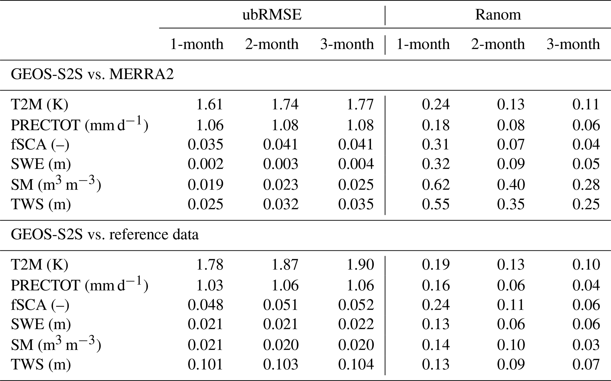
In this section, we report the results of the evaluation, showing the skill of the GEOS-S2S hydrometeorological forecasts for the HMA region. For reference, Table 2 lists the ubRMSE and the R_anom for all variables when comparing the S2S forecasts to the reanalysis (MERRA-2, Sect. 2.3) and the reference data products (Sect. 2.4). Further discussion of the results is provided in Sect. 4.

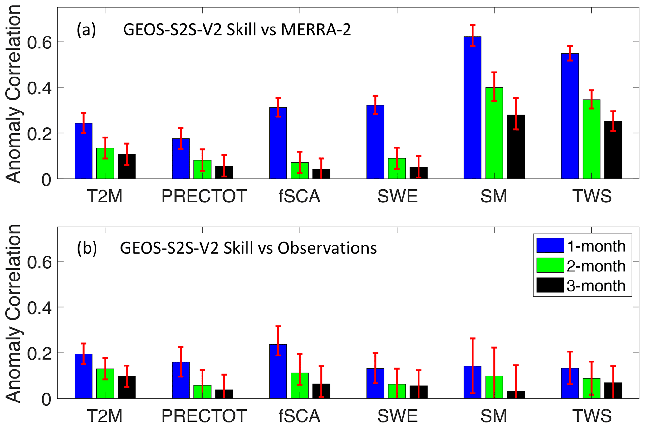
Figure 2 Anomaly correlation skill between variables for the GEOS-S2S forecasts when evaluated against MERRA-2 (a) and against reference data products (b). The evaluation of the 1-month-lead forecasts is shown in the first bar (blue), the evaluation of the 2-month-lead forecasts is shown in the second bar (green), and the evaluation of the 3-month-lead forecasts is shown in the third bar (black). The red error bars indicate the spatial standard deviation of the anomaly correlation for each variable. The reference data that are used in Figure 2B are listed in Table 1.

3.1 Difference in skill among variables and forecast lead times

Table 2 and Fig. 2 show the anomaly correlation for each variable and for each lead time considered, along with the error bars for each anomaly correlation assessment. The red error bars in Fig. 2 indicate the spatial standard deviation of the anomaly correlation for each variable. The results indicate that, across all variables, the forecast skill at 1-month lead is higher than at 2-month lead, which is higher than at 3-month lead. For example, for T2M, the 1-month forecast anomaly correlation when compared to MERRA-2 is R_anom=0.24, for the 2-month forecast it is 0.13, and for the 3-month forecast it is 0.11. And when compared to ERA5, the 1-month forecast anomaly correlation for T2M is R_anom=0.19, for the 2-month forecast it is 0.13, and for the 3-month forecast it is 0.10. Higher anomaly correlation for forecasts with a shorter lead time is seen regardless of which data product was used for the evaluation, which is aligned with other studies that evaluate S2S forecasts (e.g., Deflorio et al., 2019; Molod et al., 2020).

When comparing the S2S forecasts to MERRA-2, the variables with longer memory in the physical climate system, such as SM or TWS, have higher accuracy in the S2S forecasting system compared to variables that represent more quickly changing processes, such as T2M or PRECTOT (Fig. 2a). When the reference data products are used in the evaluation (Fig. 2b), results show that there is little evidence that variables with longer memory have higher forecast accuracy, since there is similar skill for forecasting most variables; for example, when evaluated against reference data, the range of R_anom for all variables in the verification results is 0.13 to 0.24 for the 1-month-lead forecasts.

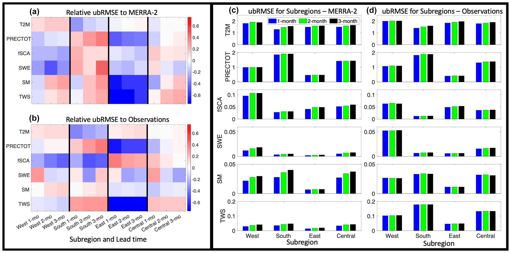
Figure 3 (a) Portrait diagram visually depicting the S2S forecast skill when evaluated against MERRA-2, comparing the skill between the different subregions (e.g., west region's 1-month forecast for T2M). Values in each box are the ubRMSE normalized by the absolute value of the climatological mean of that variable in that region (i.e., divided by the absolute value of mean T2M for the west region), normalized again by all the skill values for that climate variable (i.e., compare each metric with the normalized ubRMSE values of T2M for all subregions and all lead times). This means that if a box is blue (red), that climate variable in that subregion for that lead time has a lower (higher) normalized error when compared to that same climate variable in other subregions and lead times. (b) Same as (a) but when evaluating against other observations. (c) Errors shown here are the original ubRMSE values for each subregion when evaluating against MERRA-2, shown for all lead times and separated by climate variable. (d) Same as (c) but when evaluating against other observations.

Figure 3 shows the S2S forecast evaluation based on different subregions within the HMA domain. In Fig. 3a–b, the ubRMSE of each box is normalized by the absolute value of the climatological mean of that climate variable in that region, then it is normalized again by all the skill values for that climate variable. For example, the ubRMSE of the west region's 1-month forecast for T2M is divided by the absolute value of mean T2M in the west region (this is done to eliminate the impact of the magnitude of each climate variable in each region), then this is compared with each of the other normalized ubRMSE values of T2M for all subregions and all lead times (this is done to get a sense of which regions have more or less skill in their forecasts compared to the other regions). So, in these figures, if a box is blue (red), that climate variable in that subregion for that lead time has a lower (higher) normalized error when compared to that same climate variable in other subregions and lead times. These figures show that, for example, most variables in the east region (Inner Tibetan Plateau) have a lower normalized error when compared to the other regions. Conversely, nearly all the variables in the south region (India) have a higher normalized error than other regions. Then, in Fig. 3c–d, we show the original ubRMSE values for each subregion at all lead times, separated by climate variable. In these figures, errors can be compared for each region. For instance, fSCA and SWE have the highest error in the west region (Karakoram and Hindu Kush). Also, PRECTOT, SM, and TWS have the lowest error in the east (Inner Tibetan Plateau) region.

3.2 Annual cycles

Figure 4 shows the annual cycle, averaged over HMA, of all data products considered in this study. For T2M (Fig. 4a), the GEOS-S2S forecasts, MERRA-2, and ERA5 all have very similar annual cycles; this is persistent across lead times. The peak of the T2M annual cycle occurs during the summer months (June, July, August), reaching 290–295 K, and the low occurs during the winter months (December, January, February), dropping to 273–275 K. GEOS-S2S PRECTOT forecasts (Fig. 4b) have a wet bias compared to the MERRA-2 and APHRODITE products across nearly the entire annual cycle. The peak of all products occurs in the summer months (JJA), reaching ∼4–4.5 mm d⁻¹ for the S2S forecasts and 3.5–4 mm d⁻¹ for the evaluation products, and a low in the winter months (NDJF), dropping to 0.5–0.75 mm d⁻¹ for the S2S forecasts and 0.25–0.5 mm d⁻¹ for the evaluation products.

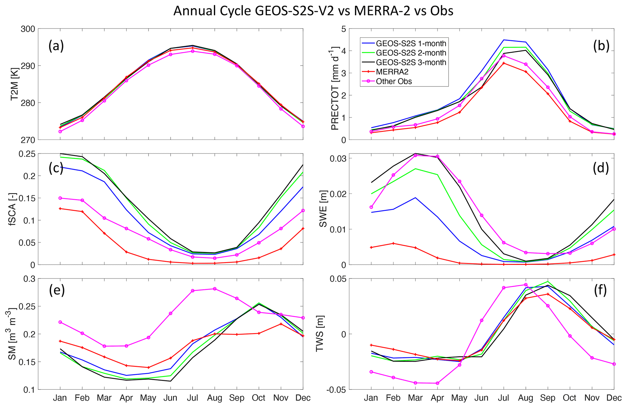
Figure 4 Annual cycle for each variable, averaged over the HMA domain. The annual cycles from the GEOS-S2S forecasts are shown for all lead times (blue, green, and black curves), and those estimated from the MERRA-2 reanalysis (red) and the reference data products (pink) are shown for comparison.

GEOS-S2S fSCA forecasts have more snow cover compared to the MERRA-2 and MODIS products, with a consistently higher mean and amplitude in the S2S forecasts (Fig. 4c). As expected, the peak of all fSCA products occurs in the winter months (DJF) and the low in the summer months (JAS); however, the magnitude and amplitude are different between the products. The peak fSCA in the S2S forecasts reaches ∼0.23–0.25, and the low is about 0.05 for the S2S forecasts; for the evaluation products, the peak is only about 0.1–0.15, with lows that are less than 0.03. Furthermore, the annual cycle of fSCA in MERRA-2 is consistently the lowest out of all the products. For SWE (Fig. 4d), the GEOS-S2S forecasts have a different annual mean and amplitude for the various lead times and in comparison to the evaluation products. The peak SWE in the S2S forecasts occurs in the spring months (March and April), reaching a high of about 0.02 m for the 1-month-lead forecasts, 0.025 m for the 2-month-lead forecasts, and 0.03 m for the 3-month-lead forecasts. For the HMA-SR product, the seasonality has a higher amplitude and magnitude, reaching a peak of ∼0.03 m in the spring months. For MERRA-2, the annual cycle of SWE is consistently lower compared to the other products, reaching a peak of ∼0.005 m in February. All products show a minimum SWE of less than 0.005 m in the summer months.

For SM, the annual cycle of the GEOS-S2S forecasts is like that of the MERRA-2 product but is substantially different from the annual cycle of the ESA-CCI data (Fig. 4e). The peak SM in the S2S forecasts occurs in the fall (∼ October) and reaches ∼0.25 m³ m⁻³, and the low occurs in the spring (around May) and drops to about 0.12 m³ m⁻³. This is similar in MERRA-2, with a peak of just over 0.2 m³ m⁻³ that occurs in November and a low of just under 0.15 m³ m⁻³ that occurs in May. For the ESA-CCI, the peak SM reaches ∼0.27 m³ m⁻³ and is observed in the summer months (JJAS) and the low drops to 0.17 m³ m⁻³ and is observed in the early spring (March). Similarly, for TWS (Fig. 4d), the annual cycle of the GEOS-S2S forecasts is like that of the MERRA-2 product but is substantially different from the annual cycles of the GRACE data. The peak of the TWS anomaly in the S2S forecasts and in MERRA-2 occurs in the late summer (ASO) and reaches ∼0.05 m, and the low occurs in the spring (April and May) and drops to about −0.02 m. For GRACE, the peak TWS reaches a high of 0.05 m in the summer (JJA) and drops to a low of −0.05 m in the spring (March–April). Therefore, there is a 1–2-month temporal lag, as well as a difference in the mean and amplitude of the annual cycles of the different products of SM and TWS between the various products considered.

3.3 Error by forecast month

The S2S forecast skill depends on various factors, such as the lead time or the variable of interest. Our results in Figs. 5 and 6 show that skill also depends on the month that is forecasted. We observe this behavior in GEOS-S2S when compared to both MERRA-2 (Fig. 5) and reference data products (Fig. 6). Note, the y axes in Figs. 5 and 6 are different so that the seasonality in each figure is properly portrayed. Figures 5 and 6 show the area-averaged error based on the forecast month of interest for each variable. As an example, the three bars for the month of April include the 1-month, 2-month, and 3-month forecasts, which are the forecasts initialized in March, February, and January respectively. These results can be suitable for those interested in understanding the errors of a forecast for a specific month, say April, using forecasts that were made 1 to 3 months prior.

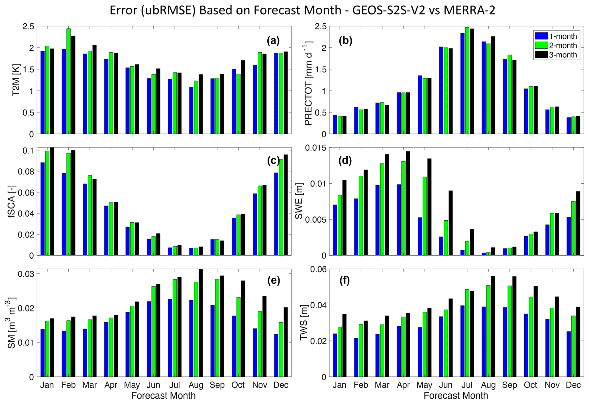
Figure 5 The expected error (ubRMSE) based on which month is forecasted. Shown here are results for 1-month (blue, first bar), 2-month (green, second bar), and 3-month (black, third bar) lead times for each variable. For example, the three bars for the month of April include the 1-month, 2-month, and 3-month forecasts, which are the forecasts initialized in March, February, and January respectively. The results displayed in this figure use MERRA-2 as the evaluation target.

We find that GEOS-S2S forecasts of T2M have less skill in the winter season, with ubRMSE greater than 2 K around February, and more skill in the summer season, with ubRMSE of less than 1.5 K around August (Figs. 5a and 6a). Errors in the precipitation forecasts are higher in the summer (July–August) compared to the winter months (December–January), with ubRMSE that is greater than 2 mm d⁻¹ in the summer and less than 0.5 mm d⁻¹ in the winter (Figs. 5b and 6b).

For the snow variables, forecasts of fSCA have higher errors in the winter season (December–February), with ubRMSE close to 0.1, and less error in the summer season (July–August), with ubRMSE of less than 0.01 (Figs. 5c and 6c). For SWE, results are different when comparing the S2S forecasts with MERRA-2 and with the HMA-SR product. Figure 5d shows that when comparing the S2S forecasts of SWE to MERRA-2, there are higher errors in the spring (March–April), with ubRMSE of 1–1.5 cm, and lower errors in the summer (August–September), with ubRMSE of less than 0.1 cm, with the forecast lead time impacting the amount of error. Yet, Fig. 6d shows that when comparing the S2S forecasts of SWE to the HMA-SR product, there are higher errors in the summer months (July–August), with ubRMSE of 4 cm, and lower errors in the fall (October–November), with ubRMSE close to 1 cm.

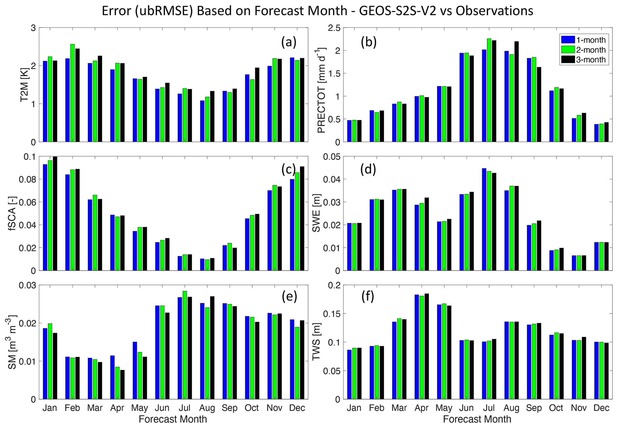
Figure 6 Same as Fig. 5, but the results displayed in this figure use the reference data products as the evaluation target. The data that are used in this figure are as follows: ERA5 for T2M, APHRODITE for PRECTOT, MODIS for fSCA, HMA-SR for SWE, ESA-CCI for SM, and GRACE for TWS.

Errors in the SM forecasts are higher in the summer (July–August) compared to the winter months (February–April), with ubRMSE values up to 0.03 m³ m⁻³ in the summer and as low as 0.01 m³ m⁻³ in the winter and spring (Figs. 5e and 6e) and with the forecast lead time impacting the magnitude of error. For TWS forecasts, results are different when comparing the S2S forecasts with MERRA-2 and with the GRACE data. Figure 5f shows that when comparing the S2S forecasts of TWS to MERRA-2, there are higher errors in the summer (around August), with ubRMSE that is over 4 cm, and lower errors in the winter (around February), with ubRMSE as low as 2 cm, with the forecast lead time impacting the magnitude of error. Yet, Fig. 6f shows that when comparing the S2S forecasts of TWS to the GRACE data, there are higher errors in the spring months (around April), with ubRMSE greater than 15 cm, and lower errors in the winter (around February), with ubRMSE below 10 cm.

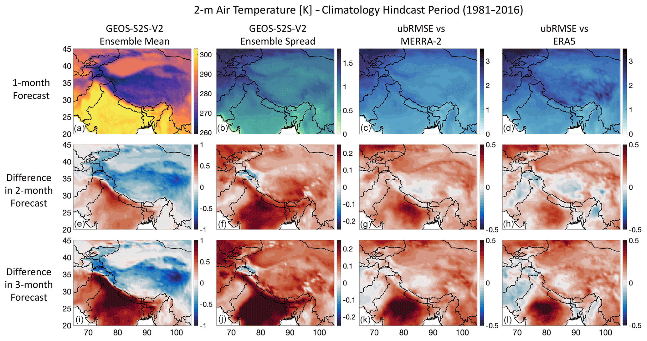
Figure 7 Screen-level (2 m) air temperature (T2M) metrics in HMA; (a) shows the climatology (long-term mean) from the GEOS-S2S 1-month forecast for the hindcast period (1981–2016); (b) shows the ensemble spread from the GEOS-S2S 1-month forecast, calculated as the standard deviation of the model ensemble at each grid cell; (c, d) show the ubRMSE when comparing the GEOS-S2S 1-month forecast to MERRA-2 and ERA5 respectively. The bottom two rows of the figures show the differences in the climatology, ensemble spread, and ubRMSE between the 2-month (e–h) and 3-month (i–l) forecasts compared to the 1-month forecast shown in the top row. Note, to calculate the difference shown in the bottom two rows, the 1-month maps in the top row are subtracted from the corresponding 2- and 3-month maps (i.e., 2-month maps minus 1-month maps and 3-month maps minus 1-month maps respectively). Therefore, red in the subfigures indicates higher values (i.e., hotter temperature, larger spread, or larger error) in the 2- and 3-month forecasts, and blue indicates lower values compared to the 1-month forecasts. The units for these plots are in K.

3.4 Spatial patterns: climatology, ensemble spread, and forecast error

This section focuses on the spatial aspect of the evaluation. Figures 7–12 show, for each variable, the GEOS-S2S ensemble mean climatology (1981–2016), the ensemble spread, the ubRMSE versus MERRA-2, and the ubRMSE versus the reference data products. The top rows of these figures show the results for the 1-month forecasts, and the middle and bottom rows show the differences in the 2-month and 3-month forecasts with respect to the 1-month forecasts.

3.4.1 Evaluation of temperature and precipitation

As expected, T2M is generally higher at lower elevations (for example, in India and Pakistan), and it is much cooler in the mountains and at higher elevations (for example, in the Himalayas and the Inner Tibetan Plateau; Fig. 7a). The ensemble spread of T2M (Fig. 7) is low compared to the ubRMSE (Fig. 7c, d), indicating that most ensemble members forecast similar T2M values. The ubRMSE is larger in regions where the spread is higher, indicating that the spatial patterns of the ensemble spread and ubRMSE are similar. The ubRMSE values relative to MERRA-2 and ERA5 show a similar magnitude throughout most of the domain, with ubRMSE values of up to ∼3 K (Fig. 7c, d). However, for the Inner Tibetan Plateau, there is more agreement with MERRA-2 (ubRMSE of ∼2 K) than with the ERA5 product (ubRMSE of ∼3 K). The 2-month (Fig. 7e) and 3-month (Fig. 7i) forecasts show a progressively warmer Indian subcontinent but are cooler in the remainder of the domain compared to the 1-month forecast. Furthermore, the ensemble spread (Fig. 7f and j) and ubRMSE (Fig. 7g, h, k, l) generally increase with increasing lead times, except for the Pakistan region. Notably, the increase in ensemble spread and error with increasing lead time is greatest in India and less pronounced for the Tibetan Plateau. These results reinforce the findings from Fig. 3 that show the evaluation based on subregions.

The mean climatology of precipitation is much wetter in parts of the domain with higher gradients of elevation, with greater than 15 mm d⁻¹ in the mountain ranges (e.g., Himalayas) and less than 5 mm d⁻¹ for other parts of the domain (Fig. 8a). Furthermore, for these same regions, the ensemble spread of PRECTOT is also much higher compared to other parts of the domain (Fig. 8b), with a mean ensemble spread up to 6 mm d⁻¹. The comparisons with MERRA-2 (Fig. 8c) and APHRODITE (Fig. 8d) both show a similar magnitude of error throughout most of the domain. The largest errors in PRECTOT forecasts are in the Indian subcontinent and in the Himalayas (ubRMSE up to 5 mm d⁻¹). This result matches the spatial interpretation of the subregion analysis shown in Fig. 3c–d. The 2-month (Fig. 8e) and 3-month (Fig. 8i) forecasts show a drier Indian subcontinent and are somewhat wetter in regions with high elevation when compared to the 1-month forecast. This difference tends to propagate to other variables shown in later figures, i.e., higher fSCA and SWE values in the mountains and lower SM and TWS values in the Indian subcontinent for 2- and 3-month forecasts compared to 1-month forecasts. Furthermore, the ensemble spread is generally higher in the mountain regions and lower over the Indian subcontinent with increasing lead time (Fig. 8f and j). For the error in precipitation, there are regions with higher error in forecasts with longer lead times, such as in India, and other regions where the error is lower with longer lead times, such as in Southeast Asia (Fig. 8g, h, k, l).

3.4.2 Evaluation of snow cover area and snow water equivalent

Snow cover is generally only found in the regions of the domain with high elevation (Fig. 9a), and there is much more snow-covered area in the northwestern parts of the domain (e.g., Hindu Kush and Karakoram). The ensemble spread of fSCA (Fig. 9b) is high for much of the domain where there is snow cover, including the Himalayas and the Inner Tibetan Plateau. The 2-month (Fig. 9e) and 3-month (Fig. 9i) forecasts show higher amounts of fSCA for much of the domain compared to the 1-month forecasts (Fig. 9a), which could be attributed to the fact that at longer lead times the forecasts are colder and wetter at higher elevations (Figs. 7 and 8a, e, i). The comparison with MERRA-2 (Fig. 9c) and MODIS (Fig. 9d) both show that errors are present where there is snow cover, where the grid cells that have no snow cover are masked out. This result matches the spatial interpretation of the subregion analysis shown in Fig. 3c–d. The error compared to MERRA-2 (ubRMSE close to 0.2) is noticeably higher than the error compared to MODIS (ubRMSE close to 0.1), especially for regions with high fSCA. This shows that GEOS-S2S fSCA is closer to what is shown in MODIS than to what is shown in the MERRA-2 product, which supports the results from Fig. 4c. Additionally, the ensemble spread (Fig. 9f, j) and the forecast errors (Fig. 9g, h, k, l) generally increase in the mountain regions with increasing lead time.

Similarly, the mean climatology of SWE (Fig. 10a) indicates that snow is present in the regions of the domain with high elevation, specifically in the major mountain ranges. Consequently, the ensemble spread of SWE (Fig. 10b) is also high in these locations (mean spread up to 0.05 m) and very low elsewhere in the domain (mean spread less than 0.01 m). The 2-month (Fig. 10e) and 3-month (Fig. 10i) forecasts show higher amounts of SWE in the major mountain ranges, which again could be attributed to the fact that at longer lead times the forecasts are colder (Fig. 7e and i) and wetter (Fig. 8e and i) in regions with high elevation gradients. The ubRMSE maps vs. MERRA-2 (Fig. 10c) and HMA-SR (Fig. 10d) show that errors are higher where there is more snow, which is expected. Again, this result matches the spatial interpretation of the subregion analysis shown in Fig. 3c–d. Here, the error compared to HMA-SR is considerably higher (ubRMSE up to 0.1 m) than the error compared to MERRA-2 (ubRMSE up to 0.04 m), especially for regions with high SWE. And like fSCA, the ensemble spread (Fig. 10f and j) and the forecast errors (Fig. 10g, h, k, l) are generally higher with increasing lead times, particularly in the major mountain ranges.

Figure 8 As in Fig. 7, but for precipitation (PRECTOT) in mm d⁻¹ and vs. APHRODITE in the right column. Here, red in the subfigures indicates lower values (i.e., less precipitation, smaller spread, or smaller error) in the 2- and 3-month forecasts, and blue indicates higher values compared to the 1-month forecasts.

3.4.3 Evaluation of soil moisture and terrestrial water storage

The mean climatology of SM (Fig. 11a) shows that soil moisture is high in India and Southeast Asia (∼0.4 m³ m⁻³) and is low in the western and northern parts of the domain (∼0.1 m³ m⁻³). There are lower SM values for forecasts with increasing lead times for the Indian subcontinent (Fig. 11e and i). This could be attributed to the fact that at longer lead times the forecasts are hotter (Fig. 7e and i) and have less precipitation (Fig. 8e and i) across the Indian subcontinent. However, for Myanmar and Southeast Asia, longer lead times produce higher SM values. The ensemble spread of SM (Fig. 11b) is lower for the 1-month forecasts and increases in magnitude for longer lead times (Fig. 11f and j). The ubRMSE maps vs. MERRA-2 (Fig. 11c) and ESA-CCI (Fig. 11d) report higher errors over regions with higher soil moisture values (ubRMSE of up to 0.06 m³ m⁻³). This result matches the spatial interpretation of the subregion analysis shown in Fig. 3c–d. Furthermore, the error increases with lead time (Fig. 11g, h, k, l), especially in India, when compared to MERRA-2 (Fig. 11g and k). However, when compared to ESA-CCI, the forecast error decreases with lead time for the western and northern parts of the domain (Fig. 11h and l). Additional data gaps are shown in these figures due to snow-covered and frozen grid cells being masked out in the S2S forecasts and due to quality control applied during post-processing of the ESA-CCI product.

The mean climatology of TWS (Fig. 12a) shows that water storage is higher in Myanmar and Southeast Asia and is lower in the other parts of the domain. The ensemble spread of TWS (Fig. 12b) is higher in the regions with a high elevation gradient (e.g., the Himalayan mountain range). Additionally, the spread of TWS is lower for the 1-month forecasts and increases in magnitude with lead time (Fig. 12f and j). The evaluation of GEOS-S2S forecasts of TWS show that the forecasts are much closer to MERRA-2 (Fig. 12c, ubRMSE less than 0.1 m) than to GRACE (Fig. 12d, ubRMSE up to 0.3 m). The errors compared to GRACE are 3–4 times higher in many regions, especially for the Indian subcontinent, Myanmar, and Southeast Asia (Fig. 12d). Again, this result matches the spatial interpretation of the subregion analysis shown in Fig. 3c–d. When compared to MERRA-2, forecasts with longer lead time (Fig. 12g and k) have higher errors, yet when compared to GRACE, there is no consistent change in the error with longer lead times (Fig. 12h and l), with some regions, such as in India, having less error with longer lead times.

4 Discussion

4.1 Role of model initialization and hydrologic persistence

S2S forecasting for HMA is in its infancy. Skill has historically been somewhat low, and as shown in our results, certain variables have high forecast skill, while others are more difficult to forecast. When comparing the S2S forecasts with MERRA-2, Figs. 2a and 3a show that the snow variables, SM, and TWS have relatively higher skill at early lead time (1 month), and for SM and TWS, this skill can persist for forecasts at longer lead times (2–3 months). This could be because GEOS-S2S and MERRA-2 have similar land conditions during initialization, both modeling systems are quite similar, and because these variables have longer persistence and memory in the physical system. When evaluating the S2S forecasts against MERRA-2, forecast skill is highest in long-memory variables (snow and soil moisture related) and lower in near-surface atmospheric variables (T2M and precipitation). In all instances, forecast skill decreases rapidly with increasing forecast lead time. When comparing the S2S forecasts with reference data products (Figs. 2b and 3b), the decline in forecast skill across lead times is slower, and the anomaly correlations are not consistently statistically different across lead times.

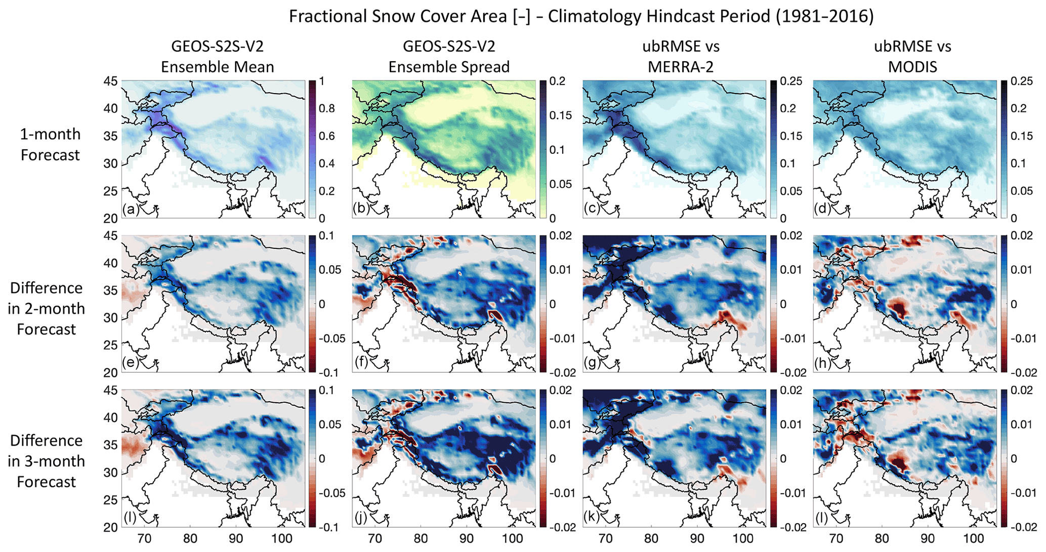
Figure 9 As in Fig. 7, but for fractional snow cover area (fSCA) (unitless) and vs. MODIS in the right column. Grid cells that are masked out (in white) show areas with no-data values. Here, red in the subfigures indicates lower values (i.e., less snow cover, smaller spread, or smaller error) in the 2- and 3-month forecasts, and blue indicates higher values compared to the 1-month forecasts.

Another reason that could explain the skill in certain variables is the role of better land surface initial conditions. For example, fSCA, SWE, SM, and TWS vary more slowly compared to T2M or PRECTOT, and their initial conditions play an important role in the skill of 1-month forecasts. This can be inferred in our results. For example, in Fig. 2a, the forecast skill relative to MERRA-2 is higher for these variables, perhaps due to similar initialization in the GEOS-S2S and MERRA-2 systems. However, in Fig. 2b, the forecast skill relative to the reference data products is not as high. Furthermore, in a more regional sense, it is possible that improvements in model initialization for SWE and SM may translate to improvements in forecast skill for the west and east subregions (Karakoram and Inner Tibet Plateau); the evidence for this is shown in Fig. 3a and b, where higher skill can be seen in the 1-month forecast for SWE and SM for these regions when evaluated against MERRA-2 compared to the evaluation against the other observations. Enhancements in forecast skill due to improved model initialization for these processes with slower temporal dynamics has been shown in other studies as well (Getirana et al., 2020; Zhou et al., 2021). Therefore, forecast skill in shorter-memory variables (T2M, PRECTOT) may increase with improvements in resolution and process representation, and gains in forecast skill for longer-memory variables (fSCA, SWE, SM, and TWS) may be achieved with improved land surface initial conditions, and if successful, increased forecast skill in 1-month lead time can propagate through to longer leads.

4.2 Reliability of S2S forecasts

Other than looking at the forecast error to determine whether a forecast was skillful or not, the spread of the forecast ensemble is another metric that gives an indication of reliability when preparing for impacts of weather events. For instance, a smaller spread in the S2S forecasts for a given region might be an indication of higher skill for that variable in that region. The results shown in this study, such as those in Figs. S1–S3 in the Supplement, provide a benchmark of information regarding the forecast skill, as well as the ensemble spread in the GEOS-S2S seasonal forecasts. Generally, one can compute the spread $/$ error ratio with the goal of that being close to 1; if it is larger than 1 (more spread than error), this is considered “under-confident”, and if it is less than 1, this is considered “overconfident” (Fortin et al., 2014). For the reliability plots in Figs. S1–S3, almost all the maps are blue, indicating that the forecasts are overconfident, meaning there is a smaller spread compared to what the error is. However, for SM (Fig. S3), this is the opposite, with red indicating that the forecasts are under-confident, meaning there is a larger spread compared to what the error is. Furthermore, for PRECTOT, fSCA, and SWE (Figs. S1–S2), there are regions in the Karakoram, Himalayas, and Inner Tibetan Plateau that also show red, indicating that the forecasts are under-confident. It is important to note, however, that there are limitations to using this reliability metric, including the fact that one can have a “perfect” ensemble prediction system with low correlation between skill and spread (see Hopson, 2014), in which case the reliability of the forecasts would be difficult to capture.

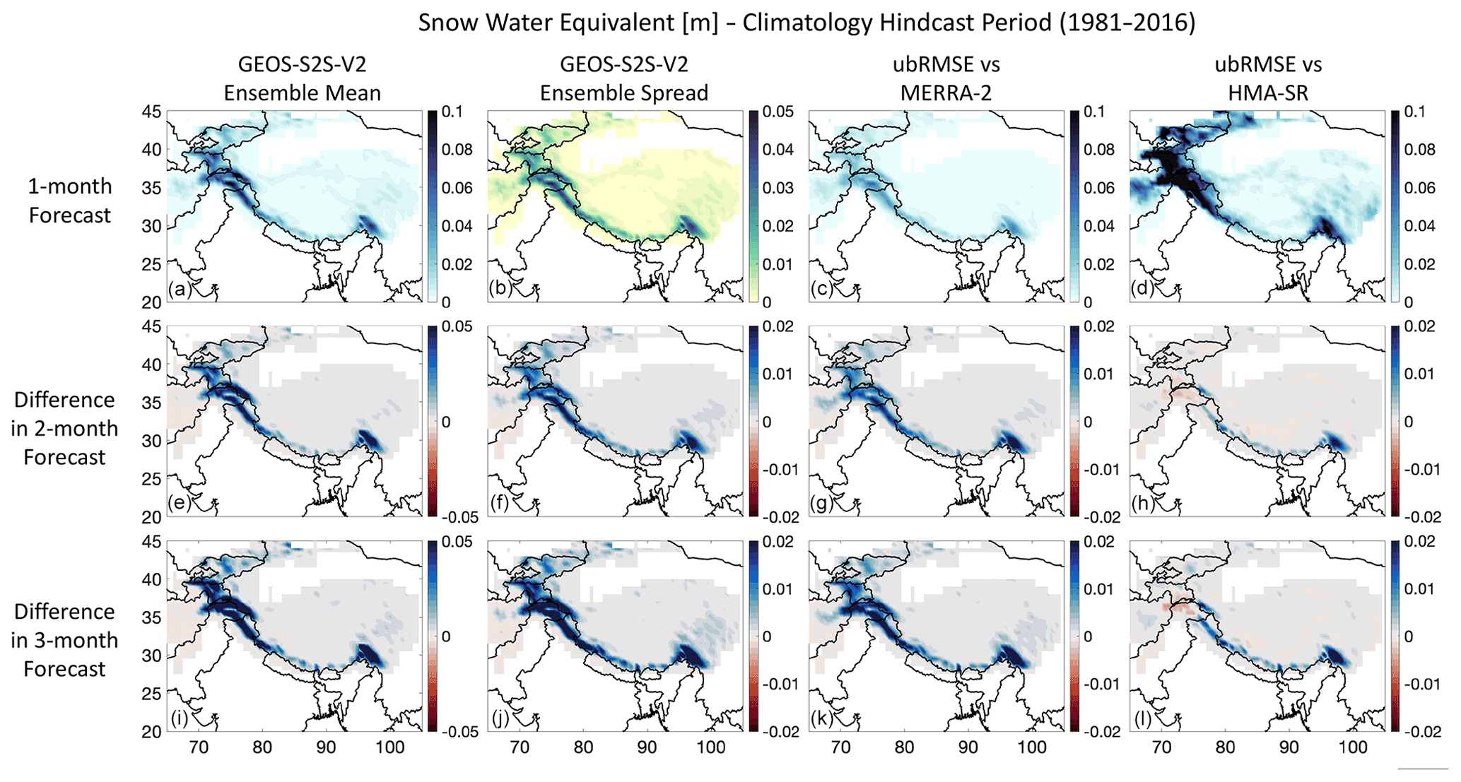
Figure 10 As in Fig. 7, but for snow water equivalent (SWE) in (m) and vs. HMA-SR in the right column. Grid cells that are masked out (in white) show areas with no-data values. Here, red in the subfigures indicates lower values (i.e., less snow water, smaller spread, or smaller error) in the 2- and 3-month forecasts, and blue indicates higher values compared to the 1-month forecasts.

4.3 The role of model characteristics

4.3.1 Resolution

For parts of the domain with high elevation and high topographic variability, many of the variables, including PRECTOT, fSCA, SWE, and TWS, had large errors (Figs. 8c–d, 9c, and 10d) and large ensemble spreads (Figs. 8b, 9b, 10b, and 12b). This is an indication of the difficulties of accurately forecasting climate for regions of high elevation and complex topography. This could be because of the coarse spatial resolution of the GEOS-S2S simulations with topography posted at a 0.5^∘ resolution (i.e., ∼50 km). The topographic smoothness in the model can impact the simulations in various ways, such as limited orographic effects or issues associated with the formation and propagation of weather events. To confirm this argument, Cannon et al. (2017) discussed the effects of topographic smoothing on the simulation of winter precipitation in HMA and found that precipitation distributions in topography that is represented in experiments with coarser resolution are biased relative to a simulation with more realistic topography. Furthermore, Zhou et al. (2021) used optimized land initial conditions from GEOS-S2S, and they were able to downscale outputs of soil moisture to 5 km resolution and to assess the forecast time horizon out to 9 months. Therefore, resolution can have a contribution to forecast skill, and it is possible that improved resolution in the S2S forecasts can help to enhance the forecast skill of certain variables.

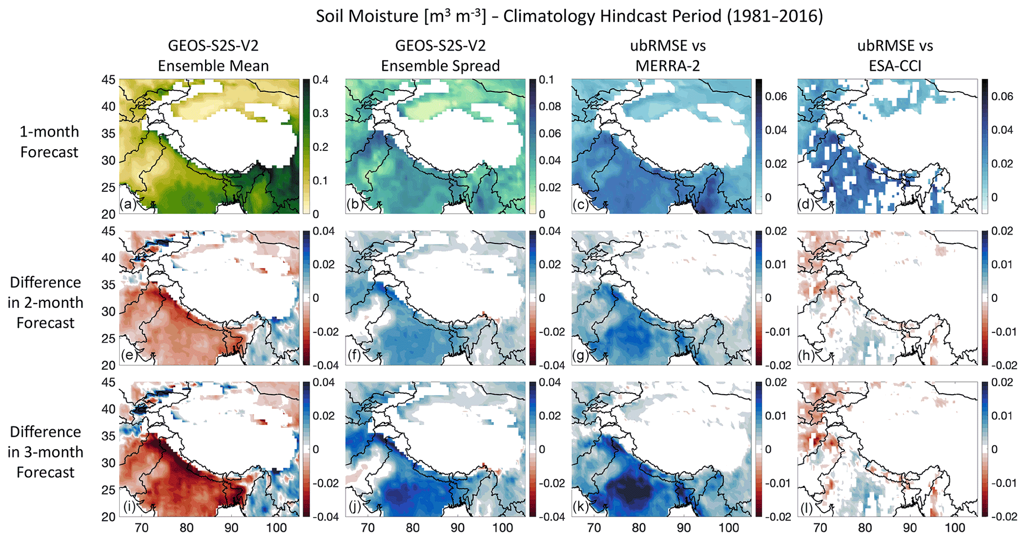
Figure 11 As in Fig. 7, but for soil moisture (SM) in (m³ m⁻³) and vs. ESA-CCI in the right column. Grid cells that are masked out (in white) show areas with no-data values. Here, red in the subfigures indicates lower values (i.e., less soil moisture, smaller spread, or smaller error) in the 2- and 3-month forecasts, and blue indicates higher values compared to the 1-month forecasts.

4.3.2 Seasonality: representing the monsoon and other atmospheric processes

S2S forecast skill largely depends on getting the seasonal signature in the forecasting system correct. In our results, there are seasonal patterns in the GEOS-S2S forecast skill (Figs. 4–6), and the simulated seasonality and the annual cycle of the hydrometeorological variables are generally well captured. For example, T2M and PRECTOT errors vary in relation to the Indian monsoon season (JJAS). Precipitation error tends to increase in these months (Figs. 5b and 6b) due to higher amounts of precipitation and because monsoon representation in the S2S system is not ideal. T2M error decreases in these months (Figs. 5a and 6a) because air temperature is most strongly related to ENSO during the monsoon season (Zhou et al., 2019), and GEOS-S2S tends to capture ENSO rather well (Molod et al., 2020; Hackert et al., 2020; Lim et al., 2021). In a regional sense, Fig. 3a and b show that errors in precipitation are generally higher for the south subregion, possibly due to the difficulties of accurately forecasting monsoon activity, which can impact precipitation in the Indian subcontinent more than in other surrounding regions. For snow variables, fSCA and SWE have low errors when snow is low during the warmest months (Figs. 5c, d and 6c). An exception is shown in Fig. 6d, where forecast errors for SWE are higher during the warm months and lower in the fall, which could be due to the forecasts accumulating SWE more rapidly in the S2S system than what is shown in the HMA-SR reanalysis product. Another explanation for this could be the role of westerly disturbances, which bring enhanced precipitation during the winter months for the west and northern parts of HMA (Cannon et al., 2016), where in our analysis the precipitation forecasts for these regions are under-confident (Fig. S1), and larger errors for fSCA (Figs. 3c, d and 9c, d) and SWE (Figs. 3c, d and 10c, d) can be expected in these regions. For SM and TWS, error patterns in Figs. 5e and f and 6e and f may be related to monsoon representation in the S2S system, but the errors can also be associated with the observational difference in the seasonal cycles shown in Fig. 4e and f. Overall, improving the representation of monsoon and westerly dynamics in GEOS-S2S may improve forecast skill, particularly during and following the monsoon season.

Our results confirm those from recent studies, such as by Deoras et al. (2021), who compared the predictions of the Indian monsoon low-pressure system in various S2S prediction models on a timescale of 15 d to ERA-Interim and MERRA-2 reanalysis data. Their study found that most models were able to predict basic features; however, all S2S models underestimated the frequency of the low-pressure systems, and precipitation biases increased with forecast lead time. Hsu et al. (2021) simulated the East Asian winter monsoon on S2S timescales for 45 d hindcasts using the Model for Prediction Across Scales (MPAS). Their evaluation results revealed that MPAS can simulate the climatological characteristics of the monsoon reasonably, with a surface cold bias for temperature and a positive rainfall bias over East Asia. However, they also found that a biased sea surface temperature may modify the circulation over the western Pacific and affect the simulated occurrence frequency of cold events near Taiwan during winter. Furthermore, climate models are notoriously known to simulate a double intertropical convergence Zone (ITCZ), in which excessive precipitation is produced on both sides of the Equator and especially in the Southern Hemisphere tropics (Hwang and Dargan, 2013; Zhang et al., 2019). This is a problem that has been persistent in climate model simulations and can impact the results of S2S forecasts in the HMA region.

4.3.3 Representation of land processes

Differences in the level of the S2S forecast skill relative to MERRA-2 and to the other reference products (Table 2 and Fig. 2) could be due to certain physical processes that are seen in the signatures of the reference data products but underrepresented in the frameworks of GEOS-S2S and MERRA-2. Characterizing hydrometeorological conditions in HMA, through both observations and modeling, is difficult owing to the scarcity of in situ observations and the complex orographic conditions that impede accurate retrievals of satellite estimates and due to properly representing these processes in the model simulations (Su et al., 2013; Ghatak et al., 2018; Loomis et al., 2019a; Yoon et al., 2019; Gerlitz et al., 2020). These challenges are reflected in the wide range of GEOS-S2S forecast skill when compared to MERRA-2 and reference datasets (i.e., as seen in Figs. 2, 4–12).

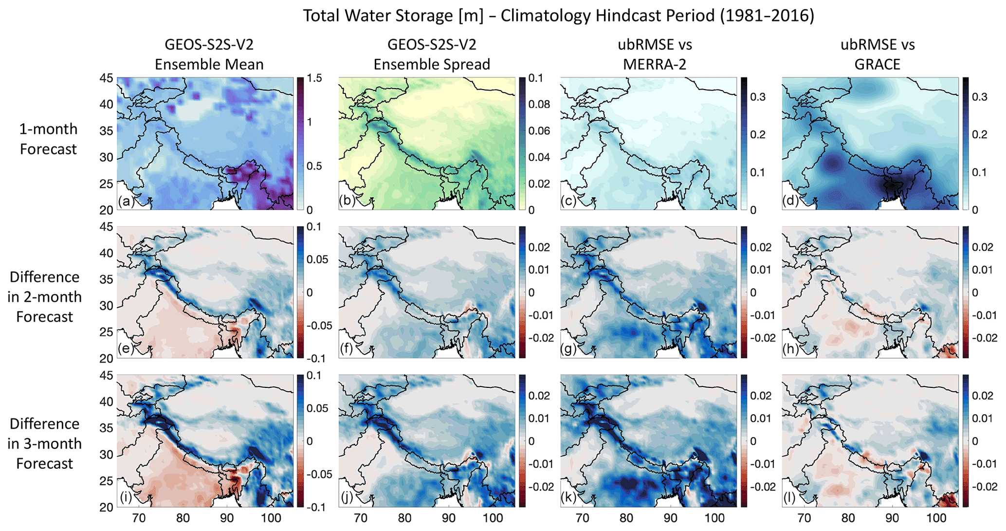
Figure 12 As in Fig. 7, but for terrestrial water storage (TWS) in (m) and vs. GRACE in the right column. Here, red in the subfigures indicates lower values (i.e., less TWS, smaller spread, or smaller error) in the 2- and 3-month forecasts, and blue indicates higher values compared to the 1-month forecasts.

For example, ESA-CCI data of SM are probably of limited quality in the topographically complex HMA region, and GRACE TWS data show the signature from rivers, lakes, glacier mass changes, and groundwater pumping that are included in GRACE data but not fully represented in the GEOS-S2S modeling framework. Some regions within HMA, particularly the Indian subcontinent, are known for intense over-pumping of groundwater, which has led to extreme levels of groundwater depletion and has played a prominent role in the loss of freshwater storage for these regions (Tiwari et al., 2009; Xiang et al., 2016; Girotto et al., 2017). This dynamic is captured in the GRACE data but not in the GEOS-S2S forecasts (i.e., compare Fig. 7c, d). More realistic representation of the various water budget components within GEOS-S2S, such as surface water or groundwater pumping, is likely to contribute to improved skill in the S2S forecasts.

Appropriate representation of seasonal snow along with temperatures and antecedent precipitation are critical to realistically forecast the HMA energy and water cycles. GEOS-S2S forecasts tend to underestimate temperature and overestimate precipitation relative to both MERRA-2 and the reference observations during all months and nearly all lead times (Fig. 4a–b); this cumulatively impacts snow cover and volume (Fig. 4c–d). MERRA-2-corrected precipitation has a known dry bias (Fig. 4b; Yoon et al., 2019), which limits fSCA and SWE accumulation in the MERRA-2 product (Fig. 4c–d). GEOS-S2S is initialized with similar land conditions to MERRA-2, resulting in low fSCA and SWE during winter 1-month-lead forecasts; however, GEOS-S2S atmospheric physics increases precipitation as forecasts continue for 2- and 3-month-lead forecasts, with more extensive snow cover and higher snow volume (Fig. 4c–d), resulting in a seasonal cycle that more closely approximates MODIS and the HMA-SR. This results in a relatively constant regional ubRMSE for all lead times when compared to MODIS and the HMA-SR (Fig. 6c–d) and localized improvements in ubRMSE with lead time across the Hindu Kush and Karakoram (Figs. 9h–l and 10h–l).

Despite the improvement in the absolute magnitude of snow volume due to increasing precipitation, limitations in the snow depletion curve used within GEOS-S2S and MERRA-2 result in more extensive snow coverage regionally and more limited reduction in fSCA relative to SWE in the Hindu Kush (Figs. 9h–l and 10h–l). Both GEOS-S2S and MERRA-2 systems use a globally consistent linear relationship between SWE and fSCA, with the minimum SWE needed to fully cover a pixel in snow; that is fSCA = 1 if SWE is greater than 26 mm (Stieglitz et al., 2001; Toure et al., 2018). This prescription was developed based on studies in the northeastern USA and oversimplifies the relationship between SWE and fSCA in mountainous regions (e.g., Schneider et al., 2021) and results in too much snow cover in the GEOS-S2S forecasts (Fig. 4c). Considering the regional pattern of the SWE–fSCA relationship, in addition to improvements in topography (Sect. 4.2.1) and inclusion of regionally important processes like surface albedo evolution, either through assimilation (Girotto et al., 2020) or directly modeling aerosol deposition on snow (Sarangi et al., 2019, 2020) will likely improve snow forecasting and associated runoff from snow melt within GEOS-S2S.

4.4 S2S forecasting for society's needs

There are various efforts in the broader community (e.g., Arendt et al., 2017) that are aimed at addressing climate change impacts on natural hazards (such as flooding or landslides) in the HMA region. S2S predictions for HMA from GEOS-S2S can potentially provide useful information for the local populations, such as by potentially providing forecasts with several-months lead time that can be beneficial in preparing for local natural hazards (Bekaert et al., 2020; Stanley et al., 2020). Different subregions within HMA can benefit in different ways from S2S forecasts based on the varying needs of local populations. Studies that utilize numerical methods and state-of-the-art model initialization to enhance S2S prediction skill are beginning to emerge. For example, Gerlitz et al. (2020) provided a review of seasonal forecasts of water availability in Central Asia. Their review showed that exceptionally skillful discharge forecasts for the agriculturally relevant vegetation season can be derived by means of statistical models taking remote-sensing-based estimations of snow coverage in the Central Asian mountain regions as independent covariates, and they found that the consideration of global climate indices, in particular El Niño, allows one to extend the forecast lead times. Therefore, there is reason to believe that improvements in S2S forecast skill can generally be achieved.

In our study, the modest levels of forecast error provide a sense of trust in the model forecasts in the context of S2S forecasting skill. For example, when compared to MERRA-2, the anomaly correlation for forecasts at 1-month lead was above 0.18 for all variables and as high as 0.62 (for SM). Relative to the reference data products, the anomaly correlation for forecasts at 1-month lead was above 0.13 for all variables and as high as 0.24 (for fSCA). Compared to other S2S evaluation studies, these results for HMA are promising. For instance, de Andrade et al. (2019) showed that anomaly correlation of global precipitation forecasts at lead times of 1 to 4 weeks was greatly reduced with lead time for a variety of S2S models, and by week 4, the anomaly correlation was consistently below 0.2 for all models. This skill level is comparable to the results presented here for the GEOS-S2S forecasts in the HMA region. Therefore, the GEOS-S2S forecasts for HMA shown in our study generally have acceptable skill at 1-month lead time compared to other S2S studies. For this study, we use multiple sources of observed and verification data to estimate the forecast skill, since relying solely on one source of information may be misleading. Here, we used two different products for each climate variable to get a sense of the uncertainty in the forecast skill for each variable. We are not aware of a merged data product for the HMA region, which would be extremely valuable for an evaluation study like this, but perhaps the combination of MERRA-2 data with other verification data products is a good alternative.

Results shown here, and from the GEOS-S2S system in general, can help the community benchmark the S2S forecasting skill for the HMA region and for specific subregions within HMA and can also help the community synthesize areas of model improvements that can potentially enhance the forecast skill or expand the time horizon of skillful forecasts. Other areas of enhancing the S2S forecasts could be achieved by the assimilation of land surface observations during the initialization period for variables such as surface soil moisture (Koster et al., 2011) or snow-covered area (Senan et al., 2016). More accurate representation of initial conditions could lead to improved forecast accuracy at the 1-month lead time, but it is possible that a gain in skill can persist for 2- and 3-month lead times and perhaps longer. Given the confluence of water resource needs from the local population and the complexity of the hydrologic cycle in HMA, further investment for improving S2S forecasts can be extremely useful for this region, and such improvements can potentially be felt globally.

5 Conclusions

We showed here an evaluation of the GEOS-S2S forecasting system in the HMA region, utilizing various products such as reanalysis data and datasets obtained from satellites or model data fusion products. The hydrometeorological variables in our evaluation results included 2 m air temperature (T2M), total precipitation (PRECTOT), fractional snow cover area (fSCA), snow water equivalent (SWE), surface soil moisture (SM), and terrestrial water storage (TWS). The main data product used for the evaluation was the MERRA-2 reanalysis product, which provided information to compare all the considered variables in GEOS-S2S. For further verification, we used separate data for the evaluation of each variable, including ERA5 for T2M, APHRODITE for PRECTOT, MODIS for fSCA, HMA-SR for SWE, ESA-CCI for SM, and GRACE for TWS. We showed various aspects of the model evaluation, such as the skill based on variables, lead time, or observation used for the evaluation. To gain a more regional point of view, we showed the evaluation based on specific subregions. We also displayed the climatology of the GEOS-S2S ensemble mean, the ensemble spread, and the mean error for each variable.

Choice of evaluation datasets heavily impacted our results. For example, when compared to MERRA-2, variables with longer memory in the physical climate system, such as soil moisture and TWS, had higher accuracy in the S2S forecasting system compared to variables representing quickly changing processes, such as temperature or precipitation. This was true when comparing the S2S forecasts to the MERRA-2 reanalysis because of similar initialization and model architecture as used in GEOS-S2S. However, this finding was not conclusive when reference data products were used in the evaluation. Finally, we provided potential avenues for model improvements that can help enhance the forecasts, such as higher-resolution topography representation and more realistic representation of surface water and groundwater pumping. These improvements can help, for example, with forecasts of TWS, since the model does not have groundwater pumping, whereas the GRACE signature includes this process. Other paths to improvement could be the assimilation of observations for the initialization of land surface state variables, such as soil moisture or snow cover.

Our results shown here benchmark the GEOS-S2S system's ability to forecast HMA on the 1–3 month timescale. We showed that, when compared to MERRA-2, the anomaly correlation for forecasts at 1-month lead was above 0.18 for all variables and as high as 0.62 (for SM). Relative to the reference data products, the anomaly correlation for forecasts at 1-month lead was above 0.13 for all variables and as high as 0.24 (for fSCA). Compared to other S2S evaluation studies, these results for HMA are promising. The reported results should motivate future improvements in the forecasts, such as model initialization, model physics, or more realistic orographic representation, that will be helpful for climate adaptation, natural hazard mitigation, and water resources planning for the population of HMA.