Interannual land cover and vegetation variability based on remote sensing data in the HTESSEL land surface model: implementation and effects on simulated water dynamics

Vegetation largely controls land surface–atmosphere interactions. Although vegetation is highly dynamic across spatial and temporal scales, most land surface models currently used for reanalyses and near-term climate predictions do not adequately represent these dynamics. This causes deficiencies in the variability of modeled water and energy states and fluxes from the land surface. In this study we evaluated the effects of integrating spatially and temporally varying land cover and vegetation characteristics derived from satellite observations on modeled evaporation and soil moisture in the Hydrology Tiled ECMWF Scheme for Surface Exchanges over Land (HTESSEL) land surface model. Specifically, we integrated interannually varying land cover from the European Space Agency Climate Change Initiative and interannually varying leaf area index (LAI) from the Copernicus Global Land Services (CGLS). Additionally, satellite data on the fraction of green vegetation cover (FCover) from CGLS were used to formulate and integrate a spatially and temporally varying effective vegetation cover parameterization. The effects of these three implementations on model evaporation fluxes and soil moisture were analyzed using historical offline (land-only) model experiments at the global scale, and model performances were quantified with global observational products of evaporation (E) and near-surface soil moisture (SM_s). The interannually varying land cover consistently altered the evaporation and soil moisture in regions with major land cover changes. The interannually varying LAI considerably improved the correlation of SM_s and E with respect to the reference data, with the largest improvements in semiarid regions with predominantly low vegetation during the dry season. These improvements are related to the activation of soil moisture–evaporation feedbacks during vegetation-water-stressed periods with interannually varying LAI in combination with interannually varying effective vegetation cover, defined as an exponential function of LAI. The further improved effective vegetation cover parameterization consistently reduced the errors of model effective vegetation cover, and it regionally improved SM_s and E. Overall, our study demonstrated that the enhanced vegetation variability consistently improved the near-surface soil moisture and evaporation variability, but the availability of reliable global observational data remains a limitation for complete understanding of the model response. To further explain the improvements found, we developed an interpretation framework for how the model development activates feedbacks between soil moisture, vegetation, and evaporation during vegetation water stress periods.

1 Introduction

Land surface–atmosphere interactions are largely controlled by vegetation, which is dynamic across spatial (local, regional, and global) and temporal (seasonal, interannual, and decadal) scales (Seneviratne et al., 2010). Land surface models (LSMs) aim to describe these interactions and are therefore a crucial aspect of models used for climate reanalysis and climate predictions. However, most state-of-the-art LSMs do not adequately represent the temporal and spatial variability of vegetation, resulting in weaknesses in the associated variability of modeled surface water and energy states and fluxes (e.g., Alessandri et al., 2007; Pitman et al., 2009; Ukkola et al., 2016; Fisher and Koven, 2020; Hersbach et al., 2020; van Oorschot et al., 2021).

To improve the representation of land surface–atmosphere dynamics, products based on satellite remote sensing data have been widely used in LSMs. Global satellite-derived maps of land cover and albedo have been directly used as boundary conditions (Faroux et al., 2013; Alessandri et al., 2017; Boussetta et al., 2021).). In addition, leaf area index (LAI) derived from satellite remote sensing has been assimilated in several LSMs for different spatial scales, generally leading to improved water, energy, and carbon fluxes (Kumar et al., 2019; Ling et al., 2019; Rahman et al., 2020, 2022). Albergel et al. (2017, 2018) also combined LAI assimilation with the assimilation of remote-sensing-based surface soil moisture in the LSM called ISBA (interactions between soil–biosphere–atmosphere). This resulted in reduced errors of modeled soil moisture, evaporation, river discharges, and gross primary production with respect to observations. Furthermore, satellite products have been used to improve model parameterizations of, for example, leaf phenology, surface roughness, soil characteristics, and subsurface water storage (Lo et al., 2010; Trigo et al., 2015; MacBean et al., 2015; Yang et al., 2016; Orth et al., 2017). Moreover, LSMs have been evaluated using global satellite products of, e.g., land surface temperatures, snow depth, and soil moisture (Balsamo et al., 2018; Johannsen et al., 2019; Dong et al., 2020; Nogueira et al., 2020, 2021; Boussetta et al., 2021).

Recent studies have exploited the latest satellite campaigns to update land cover (LC) and leaf area index (LAI) representation into the land surface model Carbon-Hydrology ECMWF Tiled Scheme for Surface Exchanges over Land (CHTESSEL) (Johannsen et al., 2019; Nogueira et al., 2020, 2021; Boussetta et al., 2021) as part of the Integrated Forecasting System (IFS) of the European Centre for Medium-Range Weather Forecasts (ECMWF). These studies replaced the original fixed map of land cover from the Global Land Cover Characteristics (GLCC) dataset representing the early 1990s (Loveland et al., 2000) with an updated map obtained from the latest-generation estimates of land cover from the European Space Agency Climate Change Initiative (ESA-CCI) (Poulter et al., 2015). Similarly, the LAI climatology from the Moderate Resolution Imaging Spectroradiometer (MODIS) (Boussetta et al., 2013) was replaced with updated climatology from the recent Copernicus Global Land Service (CGLS) LAI dataset (Verger et al., 2014). The integration of these satellite-derived variables considerably reduced the bias of model land surface temperatures (Johannsen et al., 2019; Nogueira et al., 2020, 2021). In addition, Boussetta et al. (2021) showed an overall reduction of model annual mean evaporation bias when using the updated LC and LAI in CHTESSEL.

LAI in LSMs can be coupled to the effective vegetation cover (C_eff), which characterizes the density of the vegetated surface from a top view that effectively contributes to the water and energy balances. The organization structure of leaves inside the canopy is reported as vegetation clumping. In previous modeling studies, the seasonal variations in C_eff have been described as an exponential function of LAI considering vegetation clumping in (C)HTESSEL (Alessandri et al., 2017; Nogueira et al., 2020; Boussetta et al., 2021) and in other land modeling efforts (Anderson et al., 2005; Krinner et al., 2005; Le Moigne, 2012). The shape of the exponential relation between C_eff and LAI in state-of-the-art land surface models has, to our knowledge, been assumed to be constant in time and space so far (Krinner et al., 2005; Alessandri et al., 2017; Nogueira et al., 2020; Boussetta et al., 2021). However, studies have shown that the degree of vegetation clumping, and therefore the shape of this relation, actually varies for different vegetation types (Chen et al., 2005; Ryu et al., 2010; Zhang et al., 2014).

The research gap that we identified is that most previous LSM studies using HTESSEL aimed at improving the temporally fixed boundary condition of land cover and the monthly seasonal cycle of LAI, while not exploring the effects of interannual variations of LC and LAI. Moreover, these studies have generally used one spatially fixed relationship between effective vegetation cover and LAI, while there is considerable evidence that this relationship is vegetation-type-dependent (Chen et al., 2005; Ryu et al., 2010; Zhang et al., 2014).

The objective of this research is to evaluate the effects of integrating temporal and spatial variations of land cover and vegetation characteristics derived from satellite observations on modeled evaporation and soil moisture in the land surface model HTESSEL. Specifically, we will integrate annually varying LC from ESA-CCI as well as seasonally and interannually varying LAI from CGLS. Additionally, the CGLS fraction of green vegetation cover (FCover; Verger et al., 2014) is used to formulate and implement a spatially (i.e., vegetation-dependent) and temporally (i.e., interannually) variable effective vegetation cover parameterization in HTESSEL.

2 Methods

This section describes how we integrated temporal and spatial variations of land cover and vegetation characteristics in HTESSEL. In Sect. 2.1 we describe the land cover and vegetation data used, in Sect. 2.2 we describe the model characteristics with relevance to water dynamics, and in Sect. 2.3 the model developments performed in this study are reported. Finally, the model experiments and model evaluation are described in Sect. 2.4 and Sect. 2.5, respectively.

2.1 Land cover and vegetation data

Here we used yearly land cover maps at a 300 m spatial resolution from ESA-CCI for the time period 1993–2019 (Defourny et al., 2017; Copernicus Climate Change Service, 2019). In this dataset the land cover is classified into 22 classes based on the United Nations Land Cover Classification System (LCCS) (Di Gregorio and Jansen, 2005).

LAI and FCover data were obtained from CGLS for 1999–2019 (Copernicus Global Land Service, 2022). We used the 1 km version 2 collection in which both products were derived at a 10-daily resolution from the top-of-canopy reflectance measurements by the SPOT/VEGETATION (1999–2013) and PROBA-V (2014–2019) sensors (Verger et al., 2019). These two time series were homogenized using a cumulative distribution function (CDF) approach following Boussetta and Balsamo (2021). For model spin-up purposes, the CGLS LAI (1999–2019) was further extended backwards with former-generation LAI data from the Advanced Very-High-Resolution Radiometer (AVHRR) for 1993–1999 at a 0.05^∘ resolution (Pacholczyk and Verger, 2020). The AVHRR LAI (1993–1999) was interpolated using conservative interpolation (Schulzweida, 2022) to the CGLS 1 km resolution and harmonized with CGLS (1999–2019) using CDF matching (Boussetta and Balsamo, 2021).

2.2 Relevant model components for water cycle representation

Here we used the HTESSEL land surface model (Balsamo et al., 2009) as it was developed and implemented for climate predictions with the EC-Earth3 Earth system model (Döscher et al., 2022). This version already implements a temporally, but not spatially, varying effective vegetation cover, which is further developed in this work (Alessandri et al., 2017). This section describes the relevant model representations of land cover (Sect. 2.2.1), leaf area index (Sect. 2.2.2), and effective vegetation cover (Sect. 2.2.3) in the current HTESSEL version as part of the EC-Earth3 Earth system model (ESM) and the role of these representations in the modeled water cycle. Section 2.3 describes the adaptations of these model components made in this study.

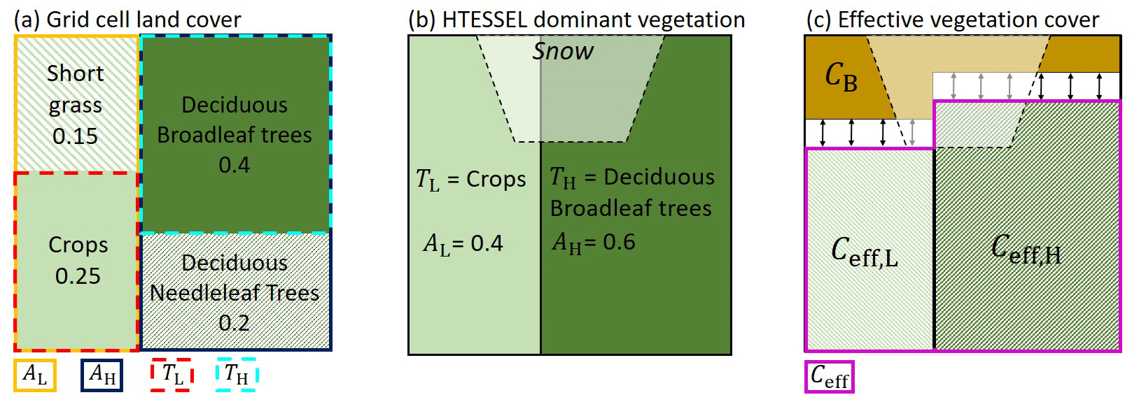
Figure 1 Vegetation representation in a grid cell with example vegetation types and cover fractions. (a) Grid cell vegetation type and cover fraction based on land cover dataset. (b) HTESSEL dominant low- and high-vegetation type (T_L and T_H) and cover fraction (A_L and A_H). (c) HTESSEL effective vegetation cover with C_eff,L and C_eff,H being the effective low- and high-vegetation cover fraction, C_B the bare soil fraction, and $C_{\mathrm{eff}}=C_{\mathrm{eff},\mathrm{L}}+C_{\mathrm{eff},\mathrm{H}}$, with the arrows indicating the temporal variability of C_eff as discussed in Sect. 2.2.3.

2.2.1 Land cover representation

In HTESSEL the vegetated area of a grid cell is divided into high- and low-vegetation tiles. In the case of snow there are separate model tiles for snow on bare ground with low vegetation and snow beneath high vegetation (Balsamo et al., 2009). Figure 1a represents an example of the vegetation types and cover fractions for a single grid cell that were originally based on the GLCC land cover dataset (Loveland et al., 2000). The low-vegetation (L) and high-vegetation (H) types with the largest cover fraction in each grid cell (see example in Fig. 1a) are used in HTESSEL as dominant vegetation types T_L and T_H (Fig. 1b). The corresponding HTESSEL vegetation cover fractions A_L and A_H are based on the total low- and high-vegetation grid cell cover fractions.

T_L and T_H directly control surface water and energy fluxes because model parameters such as vegetation root distribution, minimum canopy resistance, and roughness lengths for momentum and heat are obtained from lookup tables based on the vegetation type (ECMWF, 2015). Surface fluxes are calculated separately for low- and high-vegetation tiles and combined based on the fractions A_L and A_H. Here we only focus on the surface evaporation flux that we define as the sum of transpiration, soil evaporation, interception evaporation, and, in the case of lakes, also open-water evaporation (Savenije, 2004; Miralles et al., 2020). The subsurface in HTESSEL consists of four soil layers with thicknesses of 7, 21, 72, and 189 cm, totaling a depth of 289 cm. In this study we differentiate between near-surface soil moisture (SM_s) in the top layer (0–7 cm) and the subsurface soil moisture (SM_sb) in the three deeper layers (7–289 cm).

2.2.2 Leaf area index representation

LAI is defined separately for the high- and low-vegetation tiles (LAI_L and LAI_H). In the original HTESSEL model, LAI_L and LAI_H are prescribed as a seasonal cycle that is derived from a satellite-based climatology based on MODIS (Boussetta et al., 2013) and the vegetation cover fractions A_L and A_H. The LAI controls the canopy resistance r_c of the high- and low-vegetation tiles through the following linear relation:

$$\begin{array}{}\text{(1)}& r_{\mathrm{c}}={\displaystyle \frac{r_{\mathrm{s},\min }}{\mathrm{LAI}}}{f}_{\mathrm{1}}\left(R_{\mathrm{s}}\right)f_{\mathrm{2}}\left(D_{\mathrm{a}}\right)f_{\mathrm{3}}\left(\stackrel{\mathrm{‾}}{\mathrm{SM}}\right),\end{array}$$

with r_s,min being the prescribed vegetation-specific minimum canopy resistance that does not change in time and f₁(R_s), f₂(D_a), and $f_{\mathrm{3}}\left(\stackrel{\mathrm{‾}}{\mathrm{SM}}\right)$ being functions describing the dependencies on shortwave radiation (R_s), atmospheric water vapor deficit (D_a), and weighted average soil moisture based on the root distribution over the four soil layers ($\stackrel{\mathrm{‾}}{\mathrm{SM}}$), respectively. The effects of CO₂ changes on r_c are not explicitly taken into account in the present study. The root fractions are generally the largest in soil layers 2 and 3, and therefore transpiration mostly originates from the SM_sb. The transpiration is linearly related to r_c and atmospheric variables. Furthermore, the LAI controls the capacity of the model interception reservoir W_1 m by

$$\begin{array}{}\text{(2)}& W_{\mathrm{1}\mathrm{m}}=W_{\mathrm{1}\max }\cdot (C_{\mathrm{B}}+C_{\mathrm{L}}\cdot {\mathrm{LAI}}_{\text{L}}+C_{\mathrm{H}}\cdot {\mathrm{LAI}}_{\text{H}}),\end{array}$$

with W_1max=0.0002 m and C_B, C_L, and C_H being the fractions of bare soil, effective low vegetation, and effective high vegetation, respectively (Sect. 2.2.3). The interception evaporation per time step follows from the water content of the interception reservoir (calculated from precipitation), W_1 m, and the potential evaporation.

2.2.3 Effective vegetation cover representation

The model effective low vegetation cover and high vegetation cover (C_eff,L and C_eff,H) represent the part of the model vegetation cover fraction (A_L and A_H) that is actively contributing to the water balance through transpiration and interception evaporation (Fig. 1c). The fraction of the grid cell not covered by effective vegetation is treated as bare soil (C_B), where only soil evaporation takes place. Soil evaporation only occurs in the top soil layer (0–7 cm) and therefore originates only from SM_s. The model resistance to soil evaporation (r_soil) is described by

$$\begin{array}{}\text{(3)}& r_{\mathrm{soil}}=r_{\mathrm{soil},\min }{f}_{\mathrm{3}}\left({\mathrm{SM}}_{\mathrm{s}}\right),\end{array}$$

with $r_{\mathrm{soil},\min }=\mathrm{50}$ sm⁻¹ and f₃(SM_s) representing the dependency on the first layer soil moisture content. The effective vegetation cover fractions C_eff,L and C_eff,H as well as bare soil fraction C_B are described by

$$\begin{array}{}\text{(4)}& {\displaystyle }& {\displaystyle }{C}_{\mathrm{eff},\mathrm{L}}=c_{\mathrm{v},\mathrm{L}}\cdot A_{\mathrm{L}},\text{(5)}& {\displaystyle }& {\displaystyle }{C}_{\mathrm{eff},\mathrm{H}}=c_{\mathrm{v},\mathrm{H}}\cdot A_{\mathrm{H}},\text{(6)}& {\displaystyle }& {\displaystyle }{C}_{\mathrm{eff}}=C_{\mathrm{eff},\mathrm{L}}+C_{\mathrm{eff},\mathrm{H}},\text{(7)}& {\displaystyle }& {\displaystyle }{C}_{\mathrm{B}}=\mathrm{1}-C_{\mathrm{eff}},\end{array}$$

with c_v,L and c_v,H representing the low and high vegetation density. Originally, c_v,L and c_v,H were described by a lookup table with vegetation-specific values, allowing for spatial variation of the C_eff,L, C_eff,H, and C_B fractions. However, this approach does not represent temporal variations in vegetation density. To allow for temporal variability in C_eff (represented by the arrows in Fig. 1c), c_v,L and c_v,H were linked to the seasonal variability of LAI by the following exponential relation (Alessandri et al., 2017):

$$\begin{array}{}\text{(8)}& {\displaystyle }& {\displaystyle }{c}_{\mathrm{v},\mathrm{L}}=\mathrm{1}-e^{-k{\mathrm{LAI}}_{\text{L}}},\text{(9)}& {\displaystyle }& {\displaystyle }{c}_{\mathrm{v},\mathrm{H}}=\mathrm{1}-e^{-k{\mathrm{LAI}}_{\text{H}}},\end{array}$$

with k being the canopy light extinction coefficient that represents the degree of vegetation clumping (Anderson et al., 2005). Previously k was generally set to constant values of 0.5 (Krinner et al., 2005; Alessandri et al., 2017) or 0.6 (Boussetta et al., 2021) for all vegetation types. As a consequence, the vegetation-dependent spatial variability in k was not accounted for.

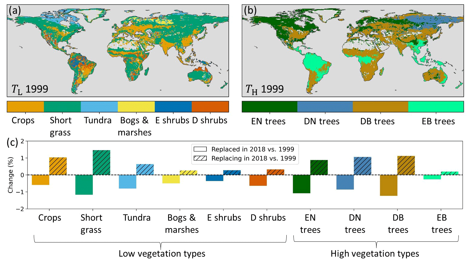
Figure 2 (a) Model low (T_L) and (b) high (T_H) dominant vegetation types in 1999 based on ESA-CCI land cover. (c) Changes in low- and high-vegetation type as a percent of the total land points, with plain colors indicating that the vegetation type was replaced in 2018 compared to 1999 and hatched colors that the vegetation replaced another type in 2018 compared to 1999. Note that low vegetation and high vegetation are treated separately and do not replace each other. E stands for evergreen, D for deciduous, N for needleleaf, and B for broadleaf.

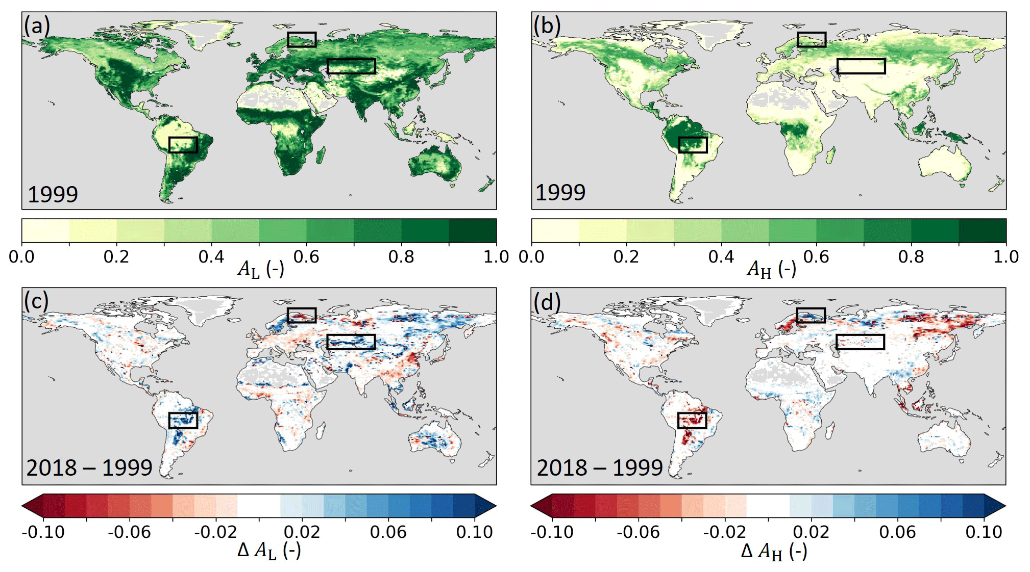
Figure 3 (a) Model low- (A_L) and (b) high-vegetation (A_H) cover fraction in 1999 as well as the absolute difference in (c) A_L and (d) A_H between 2018 and 1999 (2018–1999) based on ESA-CCI land cover. Blue (red) indicates an increased (reduced) cover in 2018. The black boxes highlight the three regions of the southern Amazon, Lapland, and central Asia that are further analyzed in Sect. 3.1.

2.3 Model developments

2.3.1 The implemented land cover variability

Here we implemented the annually varying ESA-CCI land cover (LC) data for the 1993–2019 period (Sect. 2.1), as developed by Boussetta and Balsamo (2021), for the HTESSEL vegetation types and spatial resolution. For consistency with the other model adaptations and evaluations (Sect. 2.3.2, 2.3.3 and 2.5), our LC analyses were based on 1999–2018. The interannually varying LC from ESA-CCI introduced a change in T_L in 5 % and T_H in 4 % of the land grid cells between the first (1999) and the last (2018) year of the considered study period (Fig. 2). Figure 2c shows the fraction of land grid cells in which each vegetation type (dominant in 1999) is replaced by another type in 2018 (plain colors) and conversely how often each vegetation type replaces the 1999 dominant one in 2018 (hatched colors). The figure shows that crops and short grass relatively often replaced other low-vegetation types (relatively large hatched bars), while evergreen needleleaf (EN) and deciduous broadleaf (DB) trees were relatively often replaced by other high-vegetation types (relatively large plain bars). The low- and high-vegetation cover fractions changed in many regions according to the ESA-CCI LC dataset (Fig. 3). During the 1999–2018 period, low vegetation replaced high vegetation in the southern Amazon and northeastern Siberia. Conversely, high vegetation replaced low vegetation in the boreal regions of Lapland and northwestern Siberia. Moreover, arid regions such as central Asia and Australia experienced an expansion of low vegetation over the 1999–2018 period. In Fig. 3 we highlight the southern Amazon, Lapland, and central Asia where the vegetation cover fraction changed considerably. These regions are further analyzed in Sect. 3.1.

2.3.2 The implemented leaf area index variability

We used the monthly CGLS LAI data described in Sect. 2.1 to prescribe model LAI, representing both the seasonal cycle and interannual variability of LAI. The 1 km LAI data were interpolated using conservative interpolation to the HTESSEL grid (Schulzweida, 2022). Next, LAI was disaggregated into low and high LAI (LAI_L and LAI_H) based on the low- and high-vegetation cover fractions (A_L and A_H) for use in the HTESSEL model setup with separate low- and high-vegetation tiles (Boussetta et al., 2021; Boussetta and Balsamo, 2021). Figure 4 shows the LAI interannual variability as integrated here in HTESSEL, quantified with the standard deviation. The effects of this added variability are presented in Sect. 3.2.

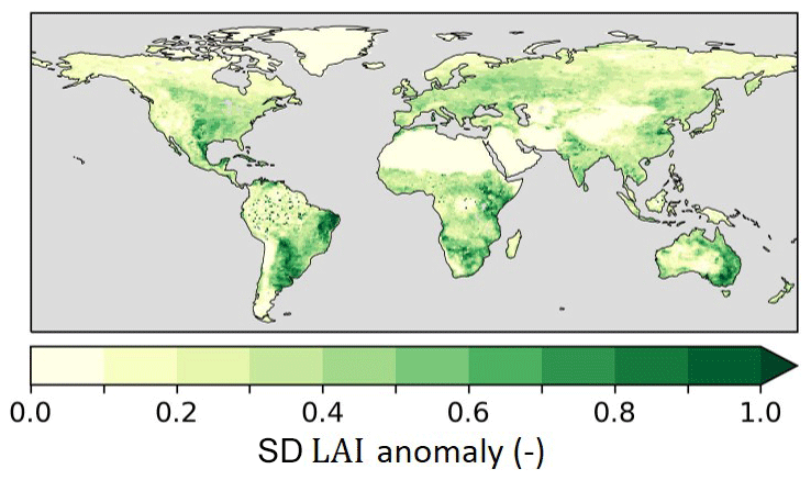
Figure 4 Standard deviation (SD) of monthly interannual anomaly CGLS LAI for 1999–2018 as implemented in experiment IAK5 (Table 1).

2.3.3 The implemented vegetation-specific effective vegetation cover parameterization

The CGLS FCover and LAI data were used (Sect. 2.1) to further develop the model effective vegetation cover parameterization as described by Eqs. (4)–(9). The constant k=0.5 parameter was replaced with a vegetation-specific k to improve spatial and temporal variability of the model C_eff. We assumed that the model C_eff is equivalent to the CGLS FCover data. Following the model C_eff parameterization, FCover is then described as follows:

$$\begin{array}{}\text{(10)}& \text{FCover}=\mathrm{1}-e^{-k\text{LAI}}.\end{array}$$

We estimated k for different HTESSEL vegetation types by solving the minimization problem in Eq. (11) using a nonlinear least-squares optimization at a 1 km spatial resolution.

$$\begin{array}{}\text{(11)}& \text{min}\Vert \mathrm{1}-e^{-k\text{LAI}}-\text{FCover}{\Vert }_{\mathrm{2}}\end{array}$$

To discriminate vegetation types, the grid cells where each vegetation type maximizes its cover fraction based on the ESA-CCI LC developed in Boussetta and Balsamo (2021) were selected for each year. For each set of grid cells corresponding to each vegetation type, the FCover and LAI 10-daily 1 km data for 1999–2019 were extracted. Here we used a 1×1 km resolution for LAI, FCover, and LC in order to obtain the most representative discrimination of vegetation types and to minimize vegetation mixing within each resolved grid cell. For the optimization of k, a randomly selected subsample of 2000 grid points of the LAI and FCover time steps (10-daily) for each vegetation type was used to keep the analysis computationally feasible, while ensuring a representative sample with robust significance of the fit. In this way, we obtained a sample of 2000 grid cells times 36 time steps per year times 20 years, which equals 1 440 000 data points to be used for the optimization for each vegetation type. This optimization resulted in vegetation-specific k values that were implemented in the HTESSEL code as in Eqs. (4)–(9). The robustness of the optimization was verified by repeating the random selection procedure several times, which resulted in negligible changes in the k estimates.

Table 1 Details of model experiments.

2.4 Model experiments

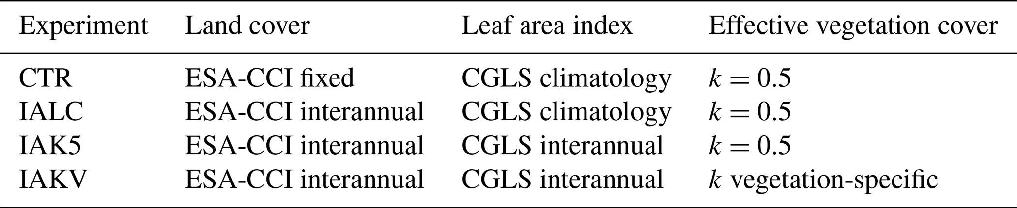
We performed experiments with an offline, uncoupled version of HTESSEL to evaluate the effect of the implemented vegetation variability as described in Sect. 2.3. HTESSEL was forced with atmospheric hourly forcing from ECMWF Reanalysis v5 (ERA5) and simulations were performed from 1993–2019, with 1993–1999 as the spin-up period (details in Table S1 in the Supplement). The model spatial resolution is the n₁₂₈ reduced Gaussian grid corresponding to grid cells of $\sim \mathrm{75}\times \mathrm{75}$ km. In total, four different model experiments were performed (Table 1). In the first experiment, as a benchmark and control experiment (CTR) the land cover of all years was set to the ESA-CCI land cover of 1993, the LAI of all years was set to the 1993–2019 climatology, and the C_eff parameterization with k=0.5 was used. This reflects standard settings of the EC-Earth3 version of HTESSEL. In the second experiment (IALC) the interannually varying ESA-CCI LC was included, while in the third experiment (IAK5) we further added interannually varying CGLS LAI. Finally, the model sensitivity to the vegetation-specific C_eff parameterization (see Sect. 2.2.3) was evaluated in the fourth experiment (IAKV). The model experiments were evaluated for 1999–2018, which is the longest period to consistently assess all three model implementations with the available evaluation data described in Sect. 2.5.

2.5 Model evaluation

2.5.1 Model variables

The effects of the vegetation-specific C_eff parameterization on the model C_eff were assessed in IAKV compared to IAK5. Furthermore, we analyzed the effects of the increasingly detailed model land cover and vegetation variability in the three experiments (IALC, IAK5, IAKV) on total evaporation (E) and the evaporation components, i.e., transpiration (E_t), soil evaporation (E_s), and interception evaporation (E_i). In addition, the effects on model near-surface soil moisture (SM_s) and subsurface soil moisture (SM_sb) were analyzed.

2.5.2 Reference data

The modeled C_eff was compared to the CGLS FCover data (Sect. 2.1) at the model spatial resolution. As a benchmark for total evaporation we used the Derived Optimal Linear Combination Evapotranspiration version 3 (DOLCEv3), which is a linear combination of estimates from ERA5-land, GLEAM v3.5a and v3.5b, and FLUXCOM-RSMETEO that was regionally weighted based on the performance in reproducing FLUXNET tower evaporation observations (Hobeichi et al., 2021). The associated uncertainty estimate is spatially and temporally varying based on the gridded evaporation and flux tower observations (Hobeichi et al., 2018). This dataset was selected because it is intended to better capture evaporation temporal variations compared to previous DOLCE versions (v1 and v2) and was therefore found to be suitable for evaluating the effects of the modified temporal and spatial variability of vegetation on evaporation (Hobeichi et al., 2021). Daily evaporation and associated uncertainty at a 0.25^∘ resolution were used for 1999–2018 and were interpolated here using conservative interpolation (Schulzweida, 2022) to the model spatial resolution.

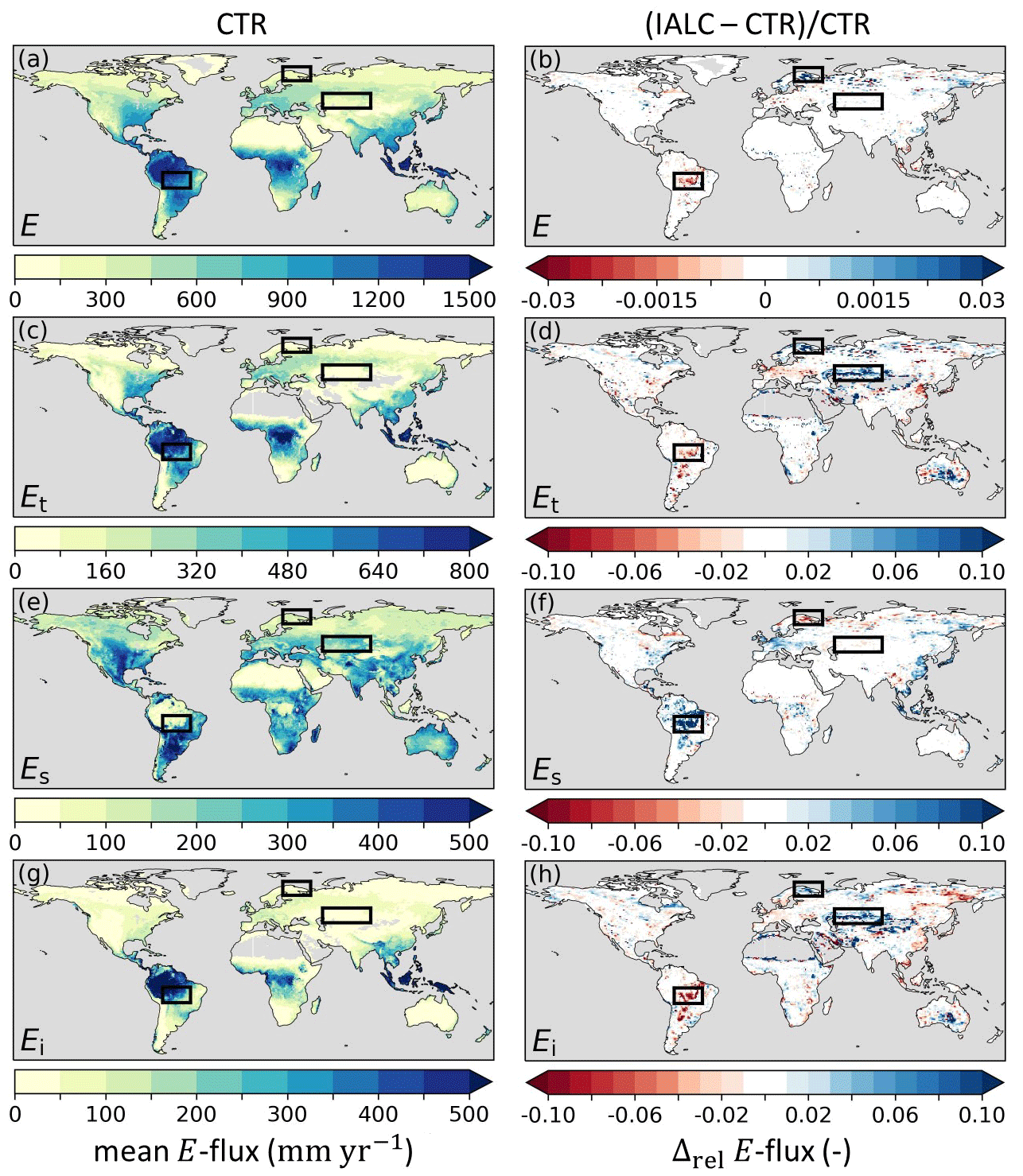
Figure 5 Annual mean evaporation fluxes (2014–2018) in experiment CTR with (a) total evaporation (E), (c) transpiration (E_t), (e) soil evaporation (E_s), and (g) interception evaporation (E_i), as well as the relative difference (Δ_rel) between annual mean evaporation fluxes in experiments IALC and CTR ((IALC−CTR)$/$CTR) for (b) E, (d) E_t, (f) E_s, and (h) E_i. Blue (red) indicates an increased (reduced) flux. Grey land areas indicate regions with annual mean E fluxes < 0.1 mm yr⁻¹. The boxes highlight the three regions of the southern Amazon, Lapland, and central Asia with major land cover changes (Fig. 3). Results with respect to DOLCEv3 E are presented in Fig. S1. See Table 1 for details of the experiments.

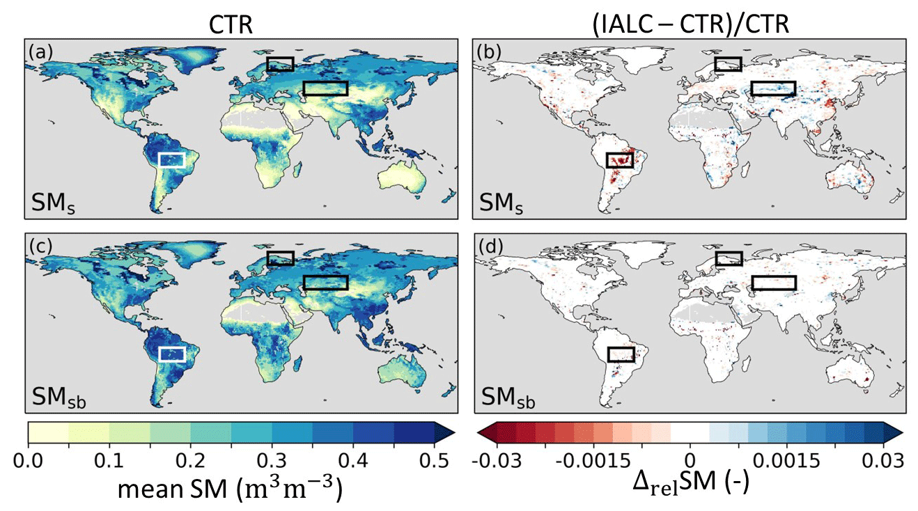
Figure 6 Annual mean soil moisture (2014–2018) (SM) in experiment CTR with (a) near-surface soil moisture (SM_s) and (c) subsurface soil moisture (SM_sb), as well as the relative difference (Δ_rel) between annual mean SM in experiments IALC and CTR ((IALC–CTR)$/$CTR) for (b) SM_s and (d) SM_sb. Blue (red) indicates increased (reduced) soil moisture. Grey land areas indicate regions with annual mean SM<0.01 m³ m⁻³. The boxes highlight the three regions of the southern Amazon, Lapland, and central Asia with major land cover changes (Fig. 3). See Table 1 for details of the experiments.

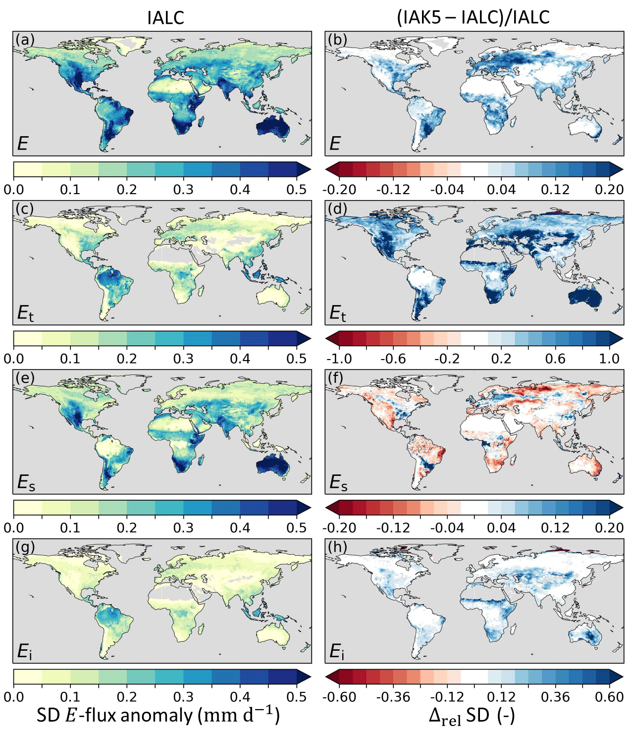
Figure 7 Standard deviation (SD) of anomaly evaporation fluxes in experiment IALC with (a) total evaporation (E), (c) transpiration (E_t), (e) soil evaporation (E_s), and (g) interception evaporation (E_i), as well as the relative difference (Δ_rel) between the anomaly E SD in experiments IAK5 and IALC ((IAK5−IALC)$/$IALC) for (b) E, (d) E_t, (f) E_s, and (h) E_i. Blue (red) indicates an increased (reduced) SD. See Table 1 for details of the experiments.

Model near-surface soil moisture (SM_s) (0–7 cm) was compared to the combined active–passive ESA-CCI soil moisture product (ESA-CCI SM v06.1), which is generated from satellite-based active and passive microwave products that are combined using the absolute values and dynamic range of the modeled soil moisture of the top 10 cm soil layer from the Global Land Data Assimilation System (GLDAS)-Noah LSM (Liu et al., 2012; Dorigo et al., 2017; Gruber et al., 2017). This dataset provides near-surface (∼0–5 cm) soil moisture at a daily resolution on a 0.25^∘ grid. Here we used the combined active–passive product interpolated using conservative interpolation (Schulzweida, 2022) to the model spatial resolution ($\sim \mathrm{75}\times \mathrm{75}$ km) for 1999–2018 (European Space Agency, 2022). The uncertainty estimates for ESA-CCI SM were also considered as they were provided with the data product and based on error variance of the data used to generate the product (Dorigo et al., 2017). ESA-CCI SM contains spatial and temporal gaps due to densely vegetated areas (tropical forests) and snow coverage. Here only grid cells with a temporal coverage larger than 60 % were used, and, as a consequence, model performance metrics for SM_s were only calculated for these grid cells.

2.5.3 Evaluation metrics

The hourly model output was first averaged to monthly values, based on which annual means, monthly climatology, and interannual anomalies were then calculated. To differentiate the seasons (June, July, and August: JJA; September, October and November: SON; December, January, and February: DJF; March, April, and May: MAM), the monthly values were averaged to seasonal means, and interannual seasonal anomalies were calculated. For the evaluation of E and SM_s with respect to reference data, we used the Pearson correlation coefficients r of the interannual monthly and seasonal anomalies. To calculate r of the interannual monthly and seasonal anomalies, the anomalies were detrended assuming a linear trend. Detrending was not applied for the effects of the modified LC, as the interannually varying LC mostly influenced the trend. In addition, we quantified the effects of the improved vegetation variability with the root mean squared error (RMSE). For C_eff and E RMSE we used monthly values, while for SM_s we used standardized interannual anomalies. Model SM_s and reference ESA-CCI SM cannot be compared directly in absolute terms due to the different representative soil layers and the imposed dynamic range from the GLDAS-Noah model (Liu et al., 2012), potentially resulting in different temporal variability (Sect. 2.5.2). To overcome this limitation, we standardized the interannual anomalies for model and reference SM_s by dividing the monthly SM_s by the climatological standard deviation.

To test the significance of the r and RMSE differences between the experiments we used a bootstrap, in which 1000 data samples were randomly created by resampling the data of model 1 and model 2 with replacement for each time step. We tested the null hypothesis that the r and RMSE of model 1 and model 2 with respect to the reference data are not significantly different from each other at the 10 % significance level.

3 Results

3.1 Land cover interannual variability effects

The interannually varying land cover from ESA-CCI in experiment IALC resulted in a shift in mean evaporation components (i.e., E_t, E_s, and E_i) compared to the CTR experiment (Fig. 5). The last 5 years of the simulations (2014–2019) are considered because the effects of the interannually varying land cover mostly emerge in this period. In the southern Amazon, where A_H was reduced on average from 0.64 to 0.57 in IALC compared to CTR (Fig. 3), the mean E_t was reduced by 3 % from 633 to 615 mm yr⁻¹ and E_i was reduced by 6 % from 384 to 363 mm yr⁻¹, while E_s increased by 17 % from 156 to 183 mm yr⁻¹. In this region, the total evaporation was reduced only by 1 % from 1174 to 1162 mm yr⁻¹ in IALC compared to CTR because the reductions in E_t and E_i were partially compensated for by increased E_s. The reduced E in IALC is closer to the DOLCEv3 E, which in this region is 1160 mm yr⁻¹. We also found an evaporation compensation effect in Lapland, where A_H increased from 0.24 to 0.30, and central Asia, where A_L increased from 0.66 to 0.71 (Fig. 3). In Lapland and in central Asia E increased by 2 % and 0.1 %, respectively, moving closer to the DOLCEv3 E (Fig. 5b; Table S2). In contrast to the small changes in E, the individual E fluxes changed considerably in these two cases (Fig. 5d, f, h).

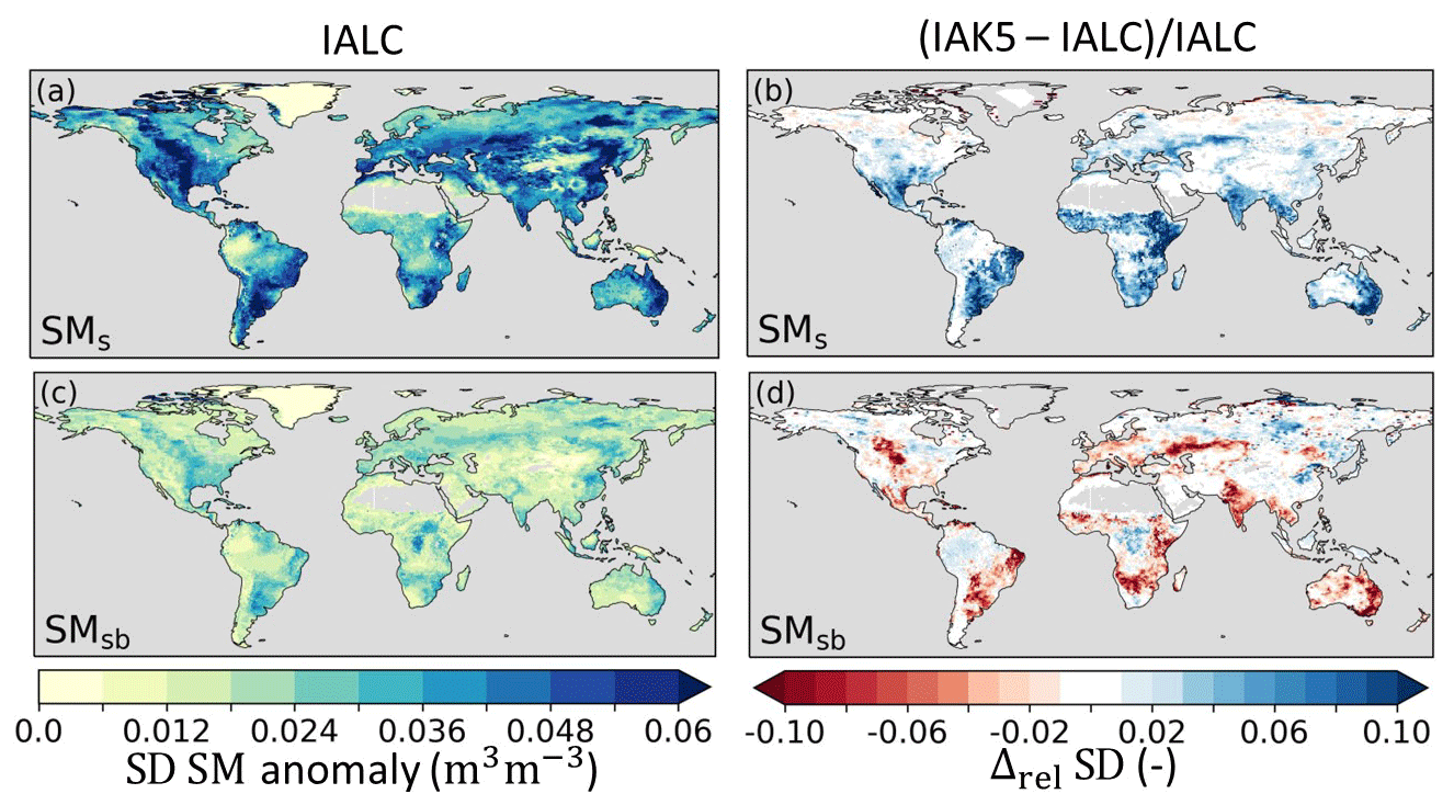
Figure 8 Standard deviation (SD) of anomaly soil moisture (SM) in experiment IALC with (a) near-surface soil moisture (SM_s) and (c) subsurface soil moisture (SM_sb), as well as the relative difference (Δ_rel) between the anomaly SM SD in experiments IAK5 and IALC ((IAK5–IALC)$/$IALC) for (b) SM_s and (d) SM_sb. Blue (red) indicates an increased (reduced) variability. See Table 1 for details of the experiments.

The changes in E_t and E_s also induced changes in soil moisture because E_s extracts water exclusively from the near-surface soil layer (SM_s), while E_t originates mostly from deeper soil layers (SM_sb). However, we observed only marginal differences between mean SM_s and SM_sb in IALC compared to CTR (Fig. 6), except for the southern Amazon SM_s. The increased E_s in the southern Amazon reduced the SM_s by 2 %, as more near-surface soil moisture was extracted (Fig. 6b). Individual evaporation fluxes influence the timing of total evaporation and soil moisture differently. However, the overall minor magnitude of changes in total E and SM_s in IALC compared to CTR led to marginal changes in RMSE and Pearson correlation coefficients with respect to the reference data in the three highlighted cases (Table S3, Figs. S1–S3).

3.2 Leaf area index interannual variability effects

The inclusion of interannual LAI variability in IAK5 (Fig. 4) generally led to an increased anomaly standard deviation (i.e., variability) of E (Fig. 7a, b). This effect is mostly dominated by E_t (Fig. 7d), which, in the model, is linearly related to LAI (Eq. 1). Figure 7d and h show that the variability in E_t and E_i was mostly increased in semiarid regions such as the Great Plains region of the US, central Asia, and southern Africa, with a stronger effect for E_t than for E_i. In contrast, the E_s variability was reduced with the enhanced LAI variability in these semiarid regions but was increased in more temperate regions such as in Europe, the eastern US, and the La Plata Basin in South America (Fig. 7e, f). While the E_t anomaly variability considerably increased in IAK5 compared to IALC in semiarid regions, the anomaly variability in subsurface soil moisture (SM_sb) that acts as the main source of E_t was reduced in these regions (Fig. 8c, d). On the other hand, the anomaly variability of SM_s increased (Fig. 8a, b), while the E_s variability was reduced.

Figure 9 shows that the Pearson correlation coefficient (r) of anomaly E with respect to DOLCEv3 increased in IAK5 compared to IALC in 85 % of the land area in which the r was significantly different in IAK5 compared to IALC. Consistently, the r of anomaly SM_s with respect to ESA-CCI SM also improved in 85 % of the significantly changing land area. For both E and SM_s r increased mostly in semiarid regions with predominantly low vegetation (Fig. 3).

3.3 Vegetation-specific effective vegetation cover parameterization effects

The observed relationship of LAI and FCover in Fig. 10 is broadly consistent with the shape of the exponential functions with the vegetation-specific k, with RMSEs between 0.018 and 0.053 for the individual vegetation types. All optimized LAI–FCover relations are characterized by k values that at 0.351–0.458 are consistently lower than the original k=0.5, which has been used as the constant default value in most HTESSEL applications so far (Alessandri et al., 2017; Boussetta et al., 2021). We found that the k values for low-vegetation types (0.438–0.458) are higher than for high-vegetation types (0.351–0.396), except for tundra regions (0.375) (Fig. 10 and Table S3). These findings are in line with our expectations, as leaf organization of low vegetation is more regular (larger k) than leaf organization of high vegetation, where leaves are found more on top of each other (smaller k) (Chen et al., 2005, 2021).

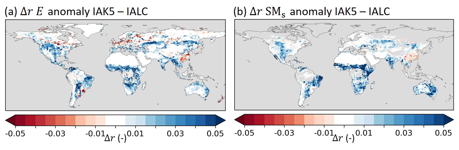
Figure 9 Pearson correlation difference (Δr) between experiments IALC and IAK5 (IAK5–IALC) for (a) monthly anomaly total evaporation (E) with respect to DOLCEv3 evaporation and (b) monthly anomaly near-surface soil moisture (SM_s) with respect to ESA-CCI SM. Blue (red) indicates an increased (reduced) correlation in IAK5 compared to IALC, white indicates small and/or insignificant Δr, and grey indicates no data points. See Table 1 for details of the experiments. Similar figures for seasonal anomalies are presented in Figs. S4–S5.

The vegetation-specific C_eff parameterization (IAKV) generally reduced the k values compared to the k=0.5 setup (IAK5), and as a consequence the associated vegetation densities c_v,L and c_v,H also decreased (Eqs. 8 and 9). On average, the global mean C_eff was reduced from 0.21 in IAK5 to 0.19 in IAKV (Fig. 11). The reduced C_eff considerably reduced the RMSE with respect to the FCover data in IAKV compared to IAK5 (Fig. 12), as expected from the parameterization optimization presented in Fig. 10. The RMSE was reduced the most over the boreal and tropical forests, with an average RMSE reduction from 0.12 to 0.06 for evergreen needleleaf trees and from 0.05 to 0.03 for evergreen broadleaf trees. On the other hand, the differences in regions with predominantly low vegetation were smaller because the fitted k value was closer to the original k=0.5, with an average RMSE reduction from 0.06 in IAK5 to 0.05 in IAKV for crops and from 0.04 to 0.03 for short grass. For low vegetation, the effects were not consistent throughout the seasons, with RMSE increasing at high latitudes in JJA (Fig. 12d). Here the C_eff in IAK5 was smaller than the CGLS FCover and is further reduced in IAKV, increasing the RMSE. This was likely caused by a poor fit for short grass at LAI > 2 (Fig. 10b) and tundra at LAI > 1 (Fig. 10g).

The reduced model C_eff in IAKV compared to IAK5 led to a shift in individual evaporation fluxes. On average, E_s increased and E_t and E_i were reduced, while the total E was not very affected (Fig. S6). These shifts led to changes in the temporal distribution of the evaporation. Figure 13 shows quite mixed results of the vegetation-specific C_eff parameterization for the model E RMSE with respect to DOLCEv3. The RMSE was consistently reduced during summer months in temperate regions such as in Europe, the eastern US, and eastern China (JJA), as well as in southeastern Brazil and southern Africa (DJF). On the other hand, the results for tropical and boreal regions were less consistent throughout the seasons (Fig. 13). The effects of the vegetation-specific C_eff on SM_s RMSE with respect to ESA-CCI SM show consistent RMSE reductions in the JJA period for Canada and southeastern Brazil and in the DJF period for the Sahel (Fig. 14). Consistent with the C_eff RMSE increase in boreal regions in JJA (Fig. 12), the Pearson correlation coefficient for monthly anomaly E with respect to DOLCEv3 E was significantly reduced in these regions in IAKV compared to IAK5, while other regions were not very affected (Fig. S14). On the other hand, the correlation of monthly anomaly SM_s with respect to ESA-CCI SM did not considerably change (Fig. S14).

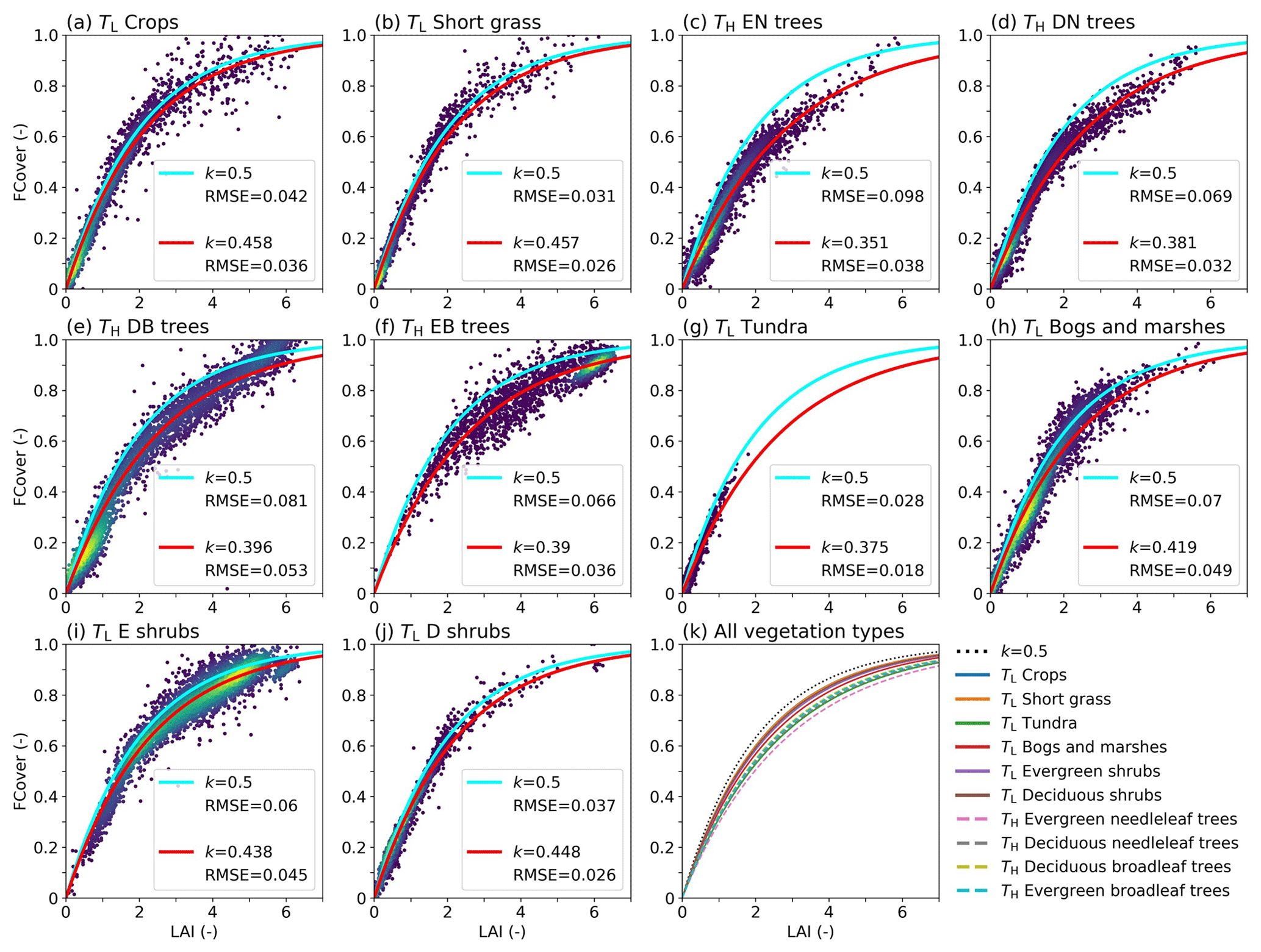
Figure 10 (a–j) LAI vs. FCover for a subsample (5000) of the selected points used for the least-squares optimization for all vegetation types with the optimized LAI–FCover relation in red (Eq. 10) and the k=0.5 relation in light blue, with RMSE values of the data points with respect to the curve. The colors indicate the point density, with purple indicating low density and yellow high density. (k) The optimized LAI–FCover relation for all vegetation types. E stands for evergreen, D for deciduous, N for needleleaf, and B for broadleaf. Values of k and RMSE are also presented in Table S3.

3.4 Combined effects of land cover, leaf area index, and effective vegetation cover

The results presented in Sect. 3.2 demonstrate that the interannually varying LAI in experiment IAK5 considerably improved the correlation of E and SM_s with respect to reference data. On the other hand, the annually varying LC and vegetation-specific C_eff affected correlations merely to a minor degree (Sect. 3.1 and 3.3). Here, we further elaborate on the effects of combining the enhanced variability in LC, LAI, and C_eff on correlation of E and SM_s.

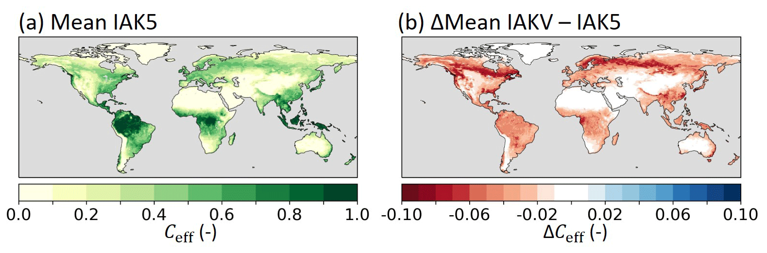
Figure 11 (a) Mean monthly model effective vegetation cover (C_eff) in experiment IAK5 and (b) the absolute difference between IAKV and IAK5 (IAKV−IAK5) mean monthly C_eff. Red (blue) indicates a reduced (increased) C_eff in IAKV compared to IAK5. Details of model experiments are in Table 1.

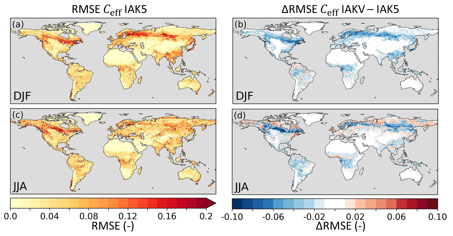
Figure 12 Root mean squared error (RMSE) of model seasonal C_eff in experiment IAK5 with respect to CGLS FCover for DJF (a) and JJA (c), with red indicating a larger RMSE. The difference between RMSE in IAK5 and IAKV (IAKV–IAK5) for DJF (b) and JJA (d) with blue (red) indicating a reduced (increased) RMSE. White indicates small and/or insignificant ΔRMSE. See Table 1 for details of the experiments. Similar figures for monthly values and all the seasons are presented in Figs. S8–S9.

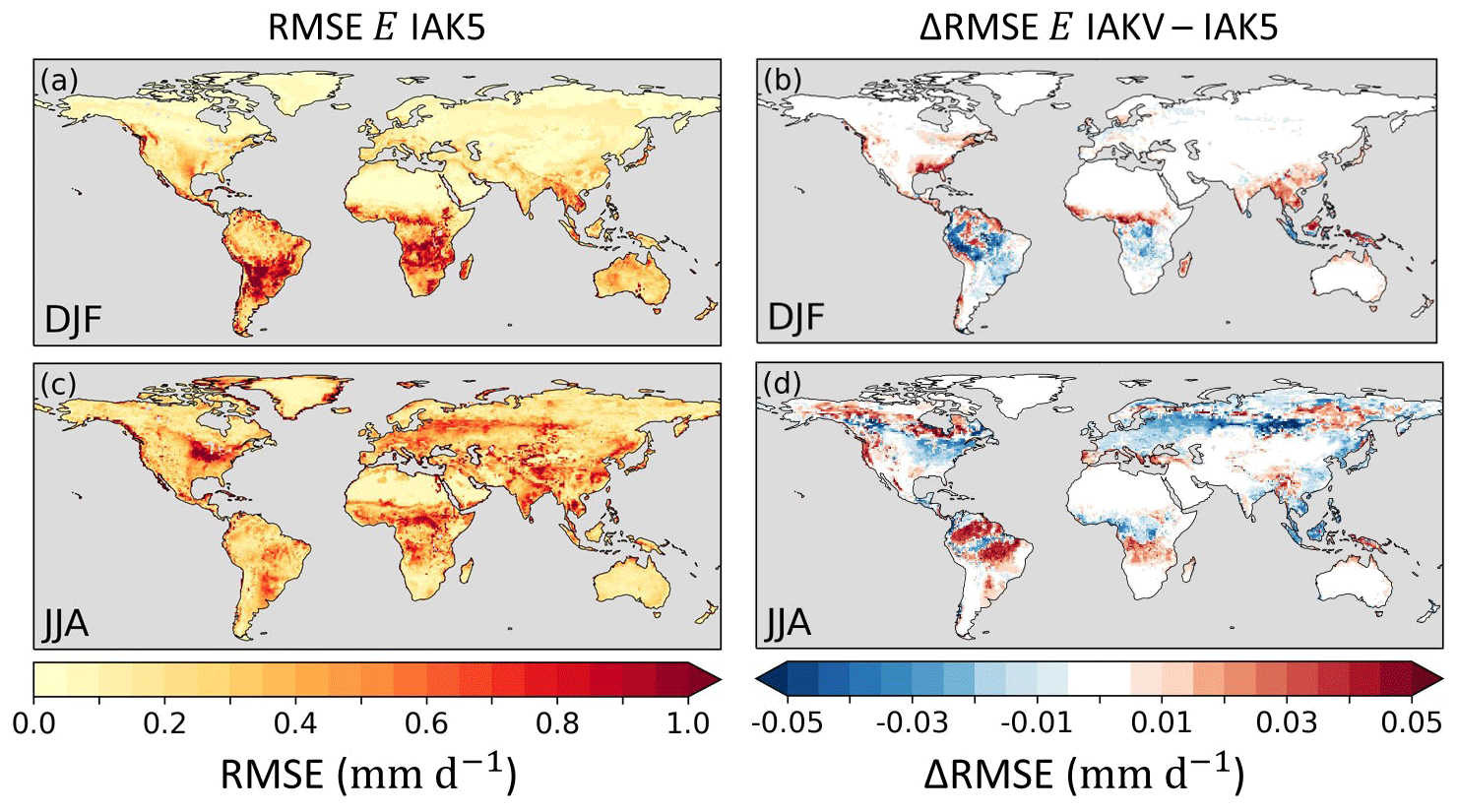
Figure 13 Root mean squared error (RMSE) of model seasonal E in experiment IAK5 with respect to DOLCEv3 E for DJF (a) and JJA (c), with red indicating a larger RMSE. The difference between RMSE in IAK5 and IAKV (IAKV–IAK5) for DJF (b) and JJA (d) with blue (red) indicating a reduced (increased) RMSE. White indicates small and/or insignificant ΔRMSE. See Table 1 for details of the experiments. Similar figures for monthly values and all the seasons are presented in Figs. S10–S11.

Figure 15 shows that the E correlation improved in 68 % (JJA) and 54 % (DJF) of the land area in which the r significantly changed in IAKV compared to CTR. Significant reduction of r is found over boreal regions, which is related to the effects of the effective vegetation cover parameterization, as discussed in Sect. 3.3 and shown in Fig. S14. Figures 15b and d show that the SM_s correlation consistently and significantly improved in 83 % (JJA) and 76 % (DJF) of the land area in which the r significantly changed in IAKV compared to CTR. The E and SM_s correlations got consistently stronger during dry periods in regions with a semiarid climate and predominantly low vegetation (Figs. 3 and 15). For example, in northeastern Brazil during the dry JJA season, the correlation coefficient for E increased from r=0.79 in CTR to 0.84 in IAKV with respect to DOLCEv3 and for SM_s from r=0.57 to 0.67 with respect to ESA-CCI SM. Similarly, in western India during the dry DJF season, the correlation coefficient for E increased from r=0.78 to 0.85 and for SM_s from r=0.45 to 0.73. To further explore the effects in these semiarid regions, we zoom in to northeastern Brazil for the 2010–2013 period (Fig. 16). This period is characterized by positive LAI and C_eff anomalies in JJA 2011 and negative LAI and C_eff anomalies in JJA 2012 (Fig. 16a, b). The negative LAI and C_eff anomalies in 2012 characterize a dry period in which the negative E anomaly was magnified in IAKV compared to CTR (Fig. 16c). During this dry period, E_t was reduced, while E_s increased. This is consistent with the soil moisture response presented in Fig. 16d, as the SM_s was reduced (due to more E_s) and the SM_sb increased (due to less E_t) during the 2012 dry period. Opposite effects were found for the 2011 period with positive LAI and C_eff anomalies. So in this specific case, the variability in E_t and SM_s anomalies was enhanced in IAKV compared to CTR, while the variability in E_s and SM_sb anomalies was dampened. This is consistent with the results presented in Figs. 7 and 8, in which the effects of the interannually varying LAI on the variability of E and SM are presented.

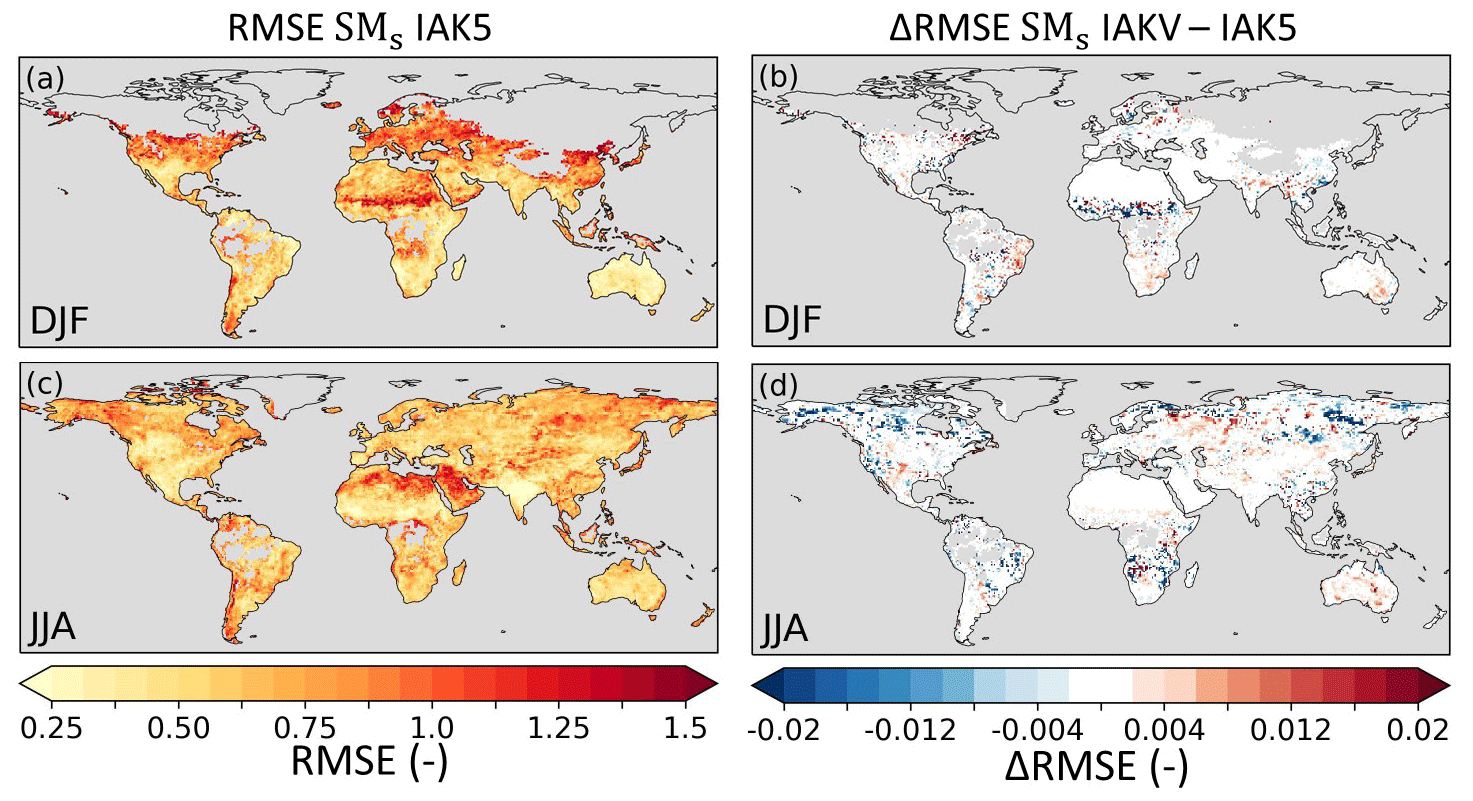
Figure 14 Root mean squared error (RMSE) of model standardized interannual seasonal anomaly SM_s in experiment IAK5 with respect to ESA-CCI SM for DJF (a) and JJA (c). The difference between RMSE in IAK5 and IAKV (IAKV–IAK5) for DJF (b) and JJA (d) with blue (red) indicating a reduced (increased) RMSE. White indicates small and/or insignificant ΔRMSE, and grey indicates no data points. See Table 1 for details of the experiments. Similar figures for monthly values and all the seasons are presented in Figs. S12–S13.

The opposing effects of the enhanced LAI variability on anomaly E_t and SM_sb can be explained by a negative feedback between vegetation and soil moisture schematized on the right side in Fig. 17a. During dry periods, the soil moisture is reduced; this lower soil water availability can result in vegetation water stress, consequently leading to lower vegetation activity in terms of transpiration and primary production, which is reflected, for example, in the typical dry season browning of grass species in low-vegetation regions and in the model represented by negative LAI and C_eff anomalies (Fig. 16a, b). As transpiration is reduced (Fig. 16c), the negative subsurface soil moisture anomaly is similarly reduced because less water is extracted (Fig. 16d). On the other hand, the enhanced vegetation variability activated a positive feedback between anomaly vegetation activity and anomaly SM_s, as illustrated on the left side of Fig. 17a. Reduced vegetation activity is reflected in the model by a reduced C_eff and an increased bare soil fraction (Sect. 7), which leads to an increased E_s (Fig. 16b) and, as a consequence, less SM_s during a dry period as long as soil moisture is available (Fig. 16d).

Figure 17b and c show that the positive feedback between E_s and SM_s, as introduced by the improved vegetation variability, is the strongest over semiarid regions with low vegetation, while the negative feedback between E_t and SM_sb is more pronounced for temperate regions with deciduous vegetation and crops, where the interannual LAI variability is larger (Fig. 4).

4 Discussion

4.1 Synthesis and implications

The results presented in Sect. 3.4 indicate overall improvements of correlation coefficients of E and SM_s with all three aspects of vegetation variability implemented. We attribute these effects primarily to the implementation of interannually varying LAI, as the effects of the LC variability and vegetation-specific C_eff on E and SM_s were smaller (Sect. 3.1 and 3.3). The pronounced improvements in SM_s and E correlation in semiarid regions (Fig. 15) are directly related to the feedback mechanisms typical of water-limited regions that were activated by the vegetation variability. Regions where the positive feedback is strong (Fig. 17b) coincide with the regions that exhibit a strengthening of the correlations. In the model setup with seasonally varying LAI only (experiments CTR and IALC), the feedbacks in Fig. 17 are not represented because the interaction between SM and LAI is activated by the interannually varying LAI. In particular, the interactions between LAI, C_eff, and bare soil cover are only captured if model C_eff is exponentially related to LAI (Sect. 2.2.3). This finding complements the arguments from previous studies for using the exponential LAI–C_eff relation instead of the lookup-table C_eff in HTESSEL (Alessandri et al., 2017; Johannsen et al., 2019; Nogueira et al., 2020, 2021).

Figure 15 Pearson correlation coefficient difference (Δr) between experiment IAK5 and IAKV (IAKV−IAK5) for (a, c) seasonal anomaly total evaporation (E) with respect to DOLCEv3 evaporation for DJF and JJA and (b, d) seasonal anomaly near-surface soil moisture (SM_s) with respect to ESA-CCI SM for DJF and JJA. Blue (red) indicates an increased (reduced) correlation in IAKV compared to IAK5, white indicates small and/or insignificant Δr, and grey indicates no data points. The red box is highlighted in Fig. 16. See Table 1 for details of the experiments. Similar figures for all the seasons and monthly anomalies are presented in Figs. S17–S19.

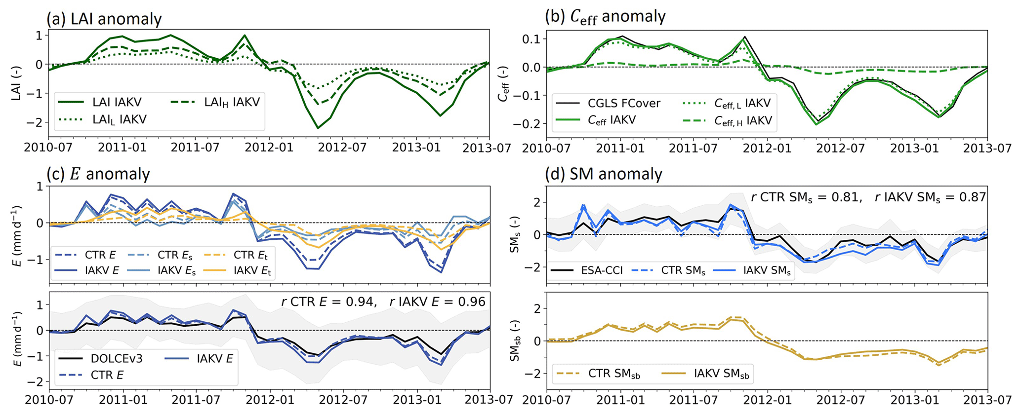
Figure 16 Time series of the northeastern Brazil case highlighted in Fig. 15 for (a) LAI anomalies. (b) Effective vegetation cover (C_eff) anomalies with the CGLS FCover data in black as a reference. (c) Evaporation anomalies with E total evaporation, E_t being transpiration, E_s soil evaporation, and E_i interception evaporation; DOLCEv3 E is in black as a reference. (d) Soil moisture standardized anomalies with SM_s near-surface soil moisture and SM_sb subsurface soil moisture; ESA-CCI SM is in black as a reference. Dashed lines in (c) and (d) represent experiment CTR and solid lines IAKV. The shading in (c) and (d) represents the uncertainty associated with the reference data. For this case T_L is short grass, T_H is deciduous broadleaf trees, A_L = 0.84, and A_H = 0.16.

Recent studies also applied data assimilation methods to integrate satellite-based LAI in LSMs. For example, Rahman et al. (2022) found improved anomaly correlations of transpiration in many areas when integrating satellite-based LAI in the LSM called Noah-MP (Noah Multi-Parameterization), with the largest effects in the regions where E and SM_s anomaly correlations consistently improved in our results (Fig. 9). However, this study also found limited sensitivity of model surface and root zone soil moisture when only LAI assimilation was applied (Rahman et al., 2022). Similarly, Albergel et al. (2017) concluded that LAI assimilation only affected deeper SM. In contrast, our results showed considerable changes in near-surface soil moisture when integrating CGLS LAI; this can be explained by the interplay between LAI, effective vegetation cover, soil evaporation, and near-surface soil moisture schematized in Fig. 17, which apparently differs from the interplay in Noah-MP (Rahman et al., 2022) and ISBA (Albergel et al., 2017).

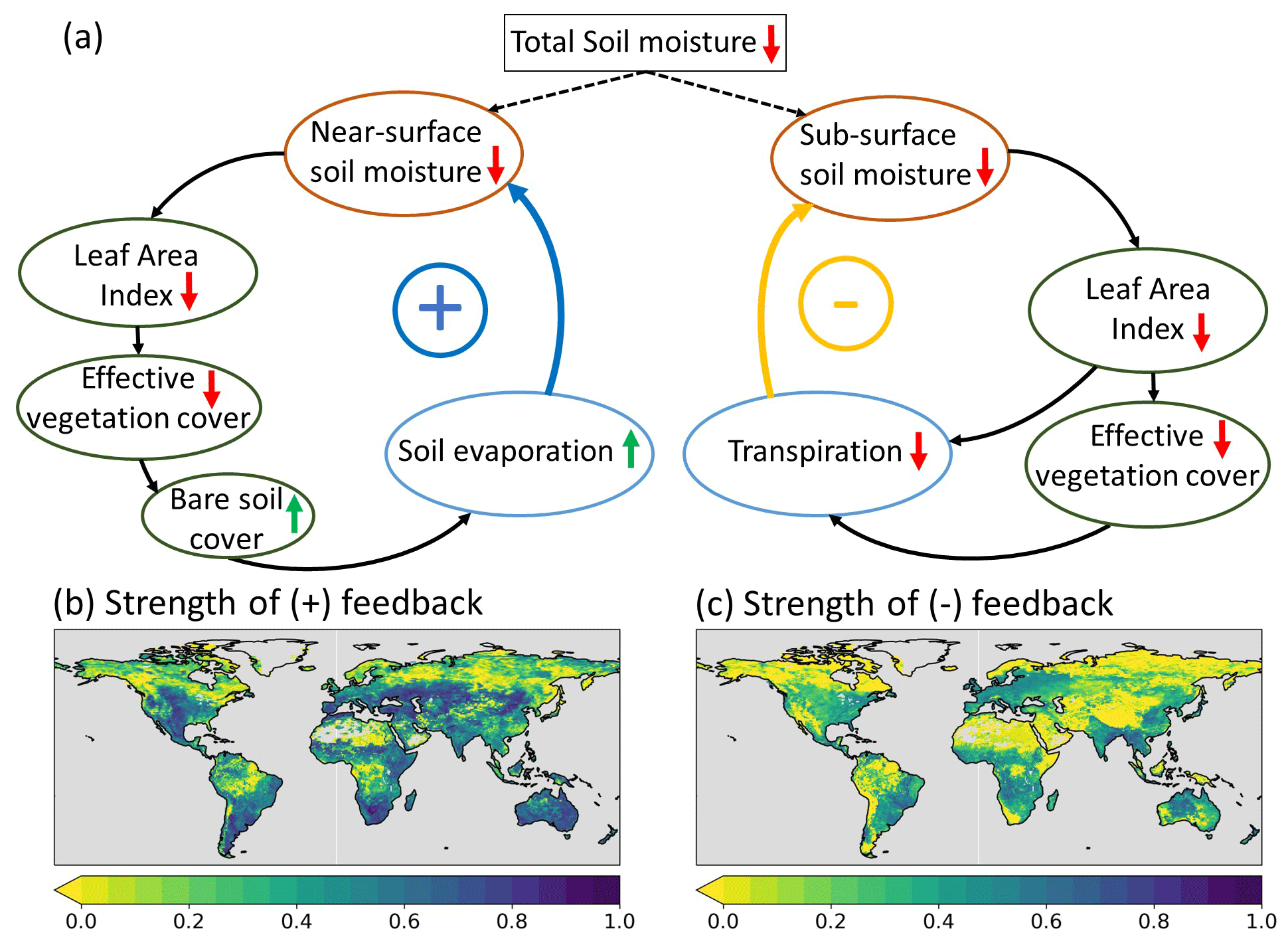
Figure 17 (a) Processes contributing to the anomaly vegetation–soil moisture feedback mechanisms as activated with the improved vegetation variability in IAKV compared to CTR. Upward (downward) arrows indicate positive (negative) change in the involved variables. Positive (blue) arrows indicate positive feedback and negative (yellow) arrows indicate negative feedback. The ± symbols refer to the resulting positive or negative feedback loop relative to the sign of the change in the involved variables. The strength of the feedbacks (b, c) is quantified as the absolute correlation between anomaly ΔE_s and ΔSM_s (b) and between ΔE_t and ΔSM_sb (c), with Δ representing the difference between anomaly CTR and IAKV (IAKV–CTR).

The vegetation-specific effective vegetation cover parameterization presented in Sect. 3.3 generally resulted in an improved match of model C_eff and CGLS FCover (Fig. 12), which was expected because the FCover data were used for the estimation of the exponential coefficient k based on least-squares minimization (Sect. 2.3.3). CGLS FCover explicitly represents the fraction of green vegetation cover and therefore matches the model actively transpiring vegetation fraction C_eff. However, the non-green vegetated area cover also affects the atmosphere by, e.g., modifying albedo and roughness lengths, which is not considered in the model, as non-green vegetation is represented as bare soil. This is a limitation for the present implementation of the vegetation-specific effective vegetation cover parameterization. The results presented in Fig. 13 showed both increased and reduced RMSE for E with respect to the reference data in IAKV compared to IAK5. Consistent reductions of E RMSE in Europe and the eastern US in the JJA period were found. These regions coincide with regions with a high density of FLUXNET tower observations used for generation of the DOLCEv3 E (Hobeichi et al., 2021). The lack of tower observations in the tropics, in the Sahel, in southeastern Asia, and at high latitudes may potentially explain the mixed RMSE results in these regions presented in Fig. 13. For high latitudes (e.g., northern Canada and eastern Siberia) the RMSE for both E as C_eff increased and the Pearson correlation was reduced (Fig. S14) in IAKV compared to IAK5 for the JJA period. This might be at least in part related to the poor fit of the parameterization for high LAI values for short grass and tundra, as explained in Sect. 3.3 (Fig. 10).

The interannually varying land cover locally affected the model E and SM as expected, with reduced (increased) E driven by corresponding reductions (increases) in high-vegetation cover fraction (Figs. 5 and 6). However, the effects on E and SM are likely underestimated due to the HTESSEL land cover structure in which the dominant vegetation type and cover fraction are used and vegetation mixing within high- or low-vegetation types is not represented (Fig. 1). With this, only major changes in the ESA-CCI vegetation types and fractions are captured by the model. In IALC we evaluated the effects of interannually varying LC individually, but for internal consistency LAI and LC interannual variations should ideally be used together as they are interdependent. The local effects of the interannually varying land cover on the total E were considerably smaller than on the individual E fluxes (Fig. 5). The reduced (increased) E_t and E_i were compensated for by increased (reduced) E_s. This compensation is related to the C_eff parameterization (Eq. 6) and also to the offline setup, which does not allow for couplings with the atmosphere. Reduced A_H in the Amazon (Fig. 3) led to a reduced C_eff and an increased bare soil fraction (Sects. 4–7) and therefore reduced E_t and E_i as well as increased E_s in order to fulfill the atmospheric evaporation demand defined by the prescribed atmospheric forcing. Similarly, the on average reduced C_eff with the vegetation-specific C_eff parameterization (Fig. 11) introduced in experiment IAKV led to a shift in annual mean individual E fluxes, with increased E_s and reduced E_t and E_i (Fig. S6).

It is important to note that the partitioning of evaporation into the three individual components E_t, E_s, and E_i in the model remains problematic to compare with observations. There is widespread consensus that, globally averaged, transpiration is the largest land evaporation flux component, followed by soil evaporation and interception evaporation (Miralles et al., 2011; Wei et al., 2017; Nelson et al., 2020). However, estimates of the average global E_t contribution to total terrestrial evaporation are subject to major uncertainties, with the global E_t contribution quantified in the range of 35 %–80 % (Schlesinger and Jasechko, 2014; Coenders-Gerrits et al., 2014). The global mean modeled partitioning of evaporation in our study is on the low end of these estimates with 39 % E_t, 38 % E_s, and 20 % E_i in CTR and 38 % E_t, 41 % E_s, and 20 % E_i in IAKV (the values do not add to 100 % due to open-water evaporation). Despite the consistent improvements in anomaly correlation coefficients of E and SM_s found in IAKV compared to CTR (Fig. 15), the apparently low contribution of E_t to total E needs further evaluation, which was out of scope in this study.

4.2 Methodological limitations

Our model experiments were performed in an offline mode with prescribed atmospheric forcing, which allowed us to analyze individual hydrological processes in detail. However, the fixed atmospheric model input considerably constrains changes in model surface fluxes. Moreover, the ERA5 forcing used here is based on an LSM that does not represent land cover and vegetation variability, which is partially corrected for by data assimilation of observations (Hersbach et al., 2020; Nogueira et al., 2021). The potential mismatch between our LSM and the ERA5 atmospheric forcing may have also influenced the observed model effects. Another possible limitation is the absence of recalibration of model parameters, such as roughness lengths and minimum stomatal resistances. Fixed model parameters were originally calibrated using the lookup-table C_eff parameterization, MODIS LAI, and GLCC LC, and they have not been adjusted for the three new model scenarios tested here (IALC, IAK5, and IAKV). This was also emphasized by Johannsen et al. (2019), Nogueira et al. (2020, 2021), and Boussetta et al. (2021), who concluded that model vegetation changes should be implemented in an integral context and recalibration of model parameters is needed.

This study emphasizes the importance of realistic representation of vegetation variability for modeling land surface–atmosphere interactions. However, for further applications exploring how the vegetation variability influences atmospheric variables in a coupled model setup is needed. The availability of reliable reference data is therefore fundamental to properly understand and model the processes of relevance for the land surface and interaction with the atmosphere. Here, the evaluation of model performance was limited to total evaporation and near-surface soil moisture. The evaluated performances of model E and SM_s need to be interpreted in a careful way, bearing in mind the uncertainties. For total evaporation we used the DOLCEv3 evaporation data that merge FLUXNET tower observations with evaporation from FLUXCOM-RSMETEO, GLEAM v3.5a and v3.5b, and ERA5-land, which all include very specific model assumptions on vegetation representations. Although these data are considered suitable for time series and trend analyses, the associated uncertainty estimates are large (Hobeichi et al., 2021) (Fig. 16). Figure 16c shows that the DOLCEv3 interannual variability is systematically smaller than the modeled variability. This limited interannual variability in DOLCEv3 could be at least in part related to the combination of several products because the averaging based on FLUXNET towers unavoidably dampens the anomalies, reducing the interannual variability. Evaluation of the modeled near-surface soil moisture was limited by missing data due to dense forests or snow cover and the lack of information on the representative soil depth. While the ESA-CCI combined active–passive SM product was generated using the absolute values and the dynamic range of GLDAS-Noah soil moisture, preserving the dynamics and trends of the original retrievals (Liu et al., 2012), it is important to note that during dry-downs the soil moisture dynamics can also be impacted to some extent, as highlighted by Raoult et al. (2022). However, we still find the ESA-CCI SM to be the best-suited globally available reference data for our study because they represent a direct product of remote sensing observations, without directly blending land surface model dynamics as done for DOLCEv3.

5 Conclusions

This study aimed to address the limitations of state-of-the-art land surface models in representing spatial and temporal vegetation dynamics. We evaluated the effects of improving the representation of land cover and vegetation variability based on satellite observational products in the HTESSEL land surface model. Specifically, we directly integrated satellite-based interannually varying land cover and seasonally and interannually varying LAI. In addition, we formulated and integrated an effective vegetation cover parameterization that can distinguish between different vegetation types. The effects of these three implementations were analyzed for soil moisture and evaporation in offline experiments forced with ERA5 atmospheric forcing.

The interannually varying land cover locally altered the model evaporation and soil moisture. In regions with major land cover changes, such as the Amazon, the model evaporation fluxes and soil moisture responded consistently, capturing the effects of increased or decreased high or low vegetation cover. The interannually varying LAI led to significant improvements of the correlation coefficients computed with the available reference data on near-surface soil moisture and evaporation. This was specifically true in semiarid regions with predominantly low vegetation during the dry season. The interannually varying LAI and effective vegetation cover allow for an adequate representation of soil moisture–evaporation feedback by activating the couplings with vegetation during vegetation-water-stressed periods (Fig. 17). From these results, we conclude that it is essential to realistically represent interannual variability of LAI and to include the exponential relation between LAI and effective vegetation cover to correctly capture land–atmospheric feedbacks during droughts in HTESSEL. The developments of the effective vegetation cover parameterization considerably improved the spatial and temporal variability of the model effective vegetation cover and regionally reduced the model errors of evaporation and near-surface soil moisture. Overall, our results emphasize the need to represent spatial and temporal vegetation variability in LSMs used for climate reanalyses and near-term climate predictions. In climate predictions, we obviously cannot rely on satellite retrievals, and therefore the development and validation of dynamical or statistical models able to reliably predict vegetation dynamics, from leaf to ecosystem scales, remain an important challenge for the future in the land surface modeling community.