the Creative Commons Attribution 4.0 License.
the Creative Commons Attribution 4.0 License.
 | 10 Nov 2023
Nonlinear time series analysis of coastal temperatures and El Niño–Southern Oscillation events in the eastern South Pacific
Berenice Rojo-Garibaldi
Manuel Contreras-López
Simone Giannerini
David Alberto Salas-de-León
Verónica Vázquez-Guerra
Julyan H. E. Cartwright
We carry out a nonlinear time series analysis motivated by dynamical systems theory to investigate the links between temperatures on the eastern South Pacific coast, influenced by the Humboldt Current System, and El Niño–Southern Oscillation (ENSO) events. To this aim, we use a set of 16 oceanic and atmospheric temperature time series from Chilean coastal stations distributed between 18 and 45∘ S. The spectral analysis indicates periodicities that can be related to both internal and external forcing, involving not only ENSO, but also the Pacific Decadal Oscillation, the Southern Annual Mode, the Quasi-Biennial Oscillation and the lunar nodal cycle. The asymptotic neural network test for chaos based on the largest global Lyapunov exponent indicates that the temperature dynamics along the Chilean coast is not chaotic. We use local Lyapunov exponents to characterize the short-term stability of the series. Using a cross-entropy test, we find that two stations in northern Chile, one oceanic (Iquique) and one atmospheric (Arica), present a significant positive cross-dependence between local Lyapunov exponents and ENSO. Iquique is the station that presents the greater number of regional characteristics and correlates with ENSO differently from the rest. The unique large-scale study area, combined with time series from hitherto unused sources (Chilean naval records), reveals the nonlinear dynamics of climate variability in Chile.
- Article
(24324 KB) - Full-text XML
- BibTeX
- EndNote


The Peru–Chile or Humboldt Current System (HCS) is a notable phenomenon of the eastern South Pacific coast. It is one of the most biologically productive eastern border oceanic currents in the world (Pauly and Christensen, 1995) as a consequence of wind-driven coastal upwellings occurring at different intensity and frequency in the southeastern Pacific (Daneri et al., 2000). Such oceanic upwelling processes also impact atmospheric temperatures (Sobarzo et al., 2007) through either local or remote effects (Hormazabal et al., 2001). Atmospheric temperatures are further affected in this region by the warm (El Niño) and cold (La Niña) phases of El Niño–Southern Oscillation (ENSO) events (Vargas et al., 2007; Enfield and Allen, 1980; Pizarro and Montecinos, 2004), and there is great interest in the possible influence of anthropogenic climate change (Sydeman et al., 2014).
A notable attempt to characterize the spatial and temporal patterns of atmospheric temperatures along the Pacific coast of South America was by Falvey and Garreaud (2009). They used in situ temperature records and satellite data for the period 1979–2006 and found that in northern and central Chile at latitudes 17–37∘ S atmospheric temperatures were cooling by about 0.20 ∘C per decade. They ascribed this cooling to a long-term La Niña phenomenon, which is consistent with the negative temperature trend observed in the Pacific Decadal Oscillation (PDO) for the same period. However, their analysis is limited to the period after satellite data became available in the mid-1970s: that is, just when two major El Niño events, in 1982–1983 and 1997–1998, took place. The effects of these large disturbances on temperature trends are not clear and have to be accounted for to provide reliable, unbiased conclusions. This is especially true for studies conducted in highly dynamic regions like the eastern South Pacific, where complex physical land–sea–atmosphere interactions suggest nonlinear relationships between coastal upwelling, interdecadal variability of El Niño-type events and global warming (Vargas et al., 2007).
In a context of global warming, it is important to understand the spatial and temporal patterns of atmospheric temperatures in complex systems like the eastern South Pacific region, since El Niño events have great impacts on human life (Glantz, 2022), and, in particular, on human health (Kovats et al., 2003) far beyond the eastern South Pacific (Fan et al., 2017). The nonlinear approach allows us to overcome many of the limitations of the linear framework. Its foundations were laid in the early 1980s, when deterministic chaos became a very active field of research (Bradley and Kantz, 2015), including in the geosciences (see e.g. Zeng et al., 2015; Nicolis and Nicolis, 1984; Grassberger, 1986; Pierrehumbert, 1990; Vassiliadis et al., 1991; Lorenz, 1991; Cuculeanu and Lupu, 2001; Petkov et al., 2015). Elsner and Tsonis (1992) and Tsonis et al. (1993) proposed that the atmosphere can be seen as a weakly coupled system and that the finite dimension of the attractor found by some of these aforementioned studies could correspond to the size of a subsystem. The dynamics of the atmosphere and the climate system is characterized by sensitivity to initial conditions (Kalnay, 2003): namely, a small error in observing the initial conditions is exponentially amplified and this implies the impossibility of mid- and long-term forecasting. This property was already recognized in the first developments of weather forecasting (Thompson, 1963) and was associated with the nonlinear nature of deterministic dynamical systems by Lorenz (1963).
In this work we study the dynamics that governs the climatic variability of the southeastern Pacific coast, its stabilities and instabilities. We discuss its consequences and its relationship with the HCS, the Pacific anticyclone, upwelling zones and the climatic phenomena that impact this region, thereby achieving a better understanding of the system's dynamics, which is impossible to achieve using linear methods. To accomplish this task, we perform a nonlinear analysis of a unique set of daily series of ambient coastal and sea surface temperatures, distributed between 18 and 45∘ S and spaced every 3 to 4∘ of latitude. We test in a mathematically rigorous fashion for the presence of chaotic dynamics through the largest Lyapunov exponent. In addition, we characterize the local stability of the systems using local Lyapunov exponents (LLEs), which quantify the state-dependent predictability over finite time horizons. Also, we study how the dynamics is affected by ENSO events by comparing LLEs and the Oceanic Niño Index in different latitudes of the Chilean coast. Finally we discuss the periodicities of the time series, the type of dynamics involved and the bioclimatic characteristics found by latitude in order to understand the role played by both internal and external forcing in the climatic variability of the eastern South Pacific.
Table 1Daily and weekly data for oceanic stations.
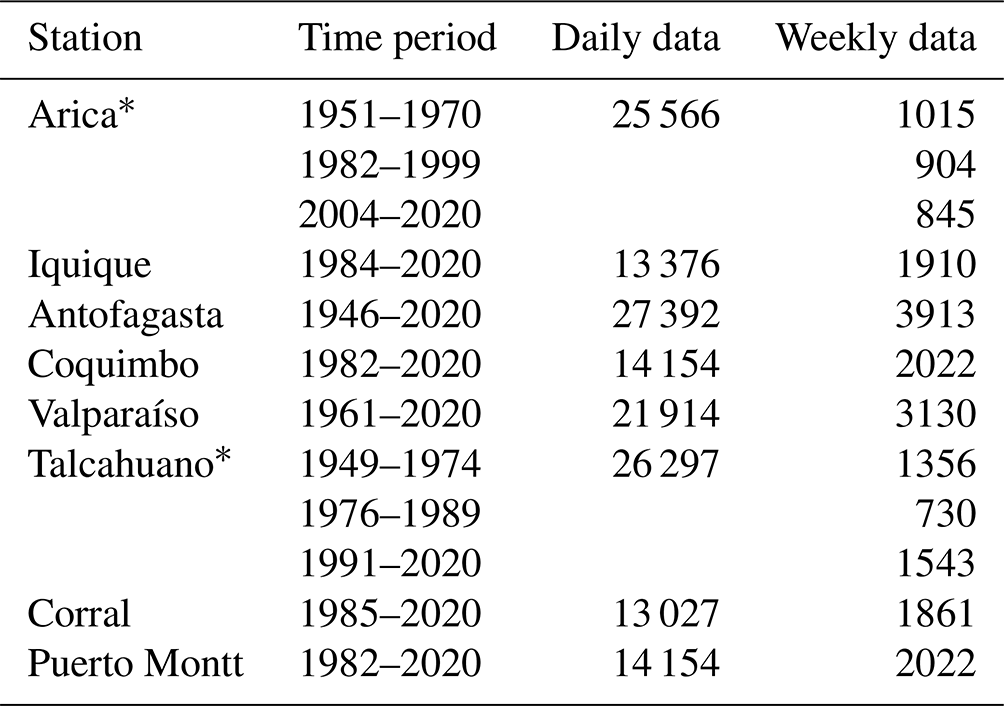
∗ The data are split into three series due to the presence of gaps.
Table 2Daily and weekly data for atmospheric stations.
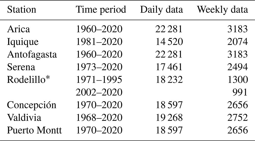
∗ The data are split into two series due to the presence of gaps.
2.1 Data pre-processing
Sea surface temperature (SST) data were obtained from the Hydrographic and Oceanographic Service of the Chilean Navy (SHOA), which has kept records for the main ports of the country since the mid-20th century. Data on atmospheric surface temperature (AST) begin from the first half of the 20th century and were provided by the Meteorological Directorate of Chile (DMC). Since the DMC weather stations are associated with the presence of airports in major cities, they usually coincide with the main ports. For all stations, the daily data were converted to weekly average temperature time series. In the case of missing data, we applied Kalman filtering for imputation using the R package imputeTS
(Moritz and Bartz-Beielstein, 2017). Tables 1 and 2 list the oceanic and atmospheric stations used in this study. The first column contains the location names that range from the northern to the southern regions of Chile and the second column indicates the time range; the third and fourth columns report the sample sizes.
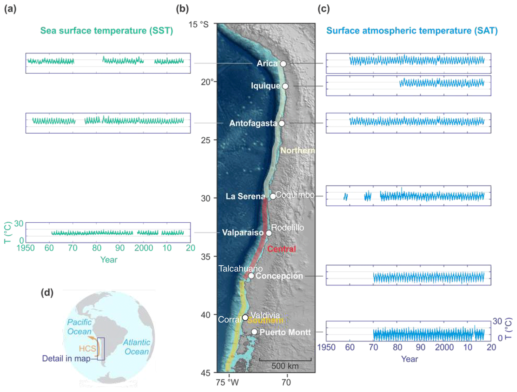
Figure 1Study area and examples of time series used in this work. (a) Sea surface temperature for stations from northern to southern Chile. (b) Study area. (c) Atmospheric surface temperature for the same region. (d) Study area relative to the Humboldt Current System (HCS). For comparative purposes, all the time series plots here use the same temperature scale and timescale.
2.1.1 Study area
Along the southeastern Pacific littoral between 18 and 45∘ S there is a marked climatic gradient from an arid zone to a rainy Mediterranean zone. Three major divisions are identifiable along the coast of Chile (Sarricolea et al., 2017): the north at 18–30∘ S, the centre at 30–37∘ S and the south at 37–45∘ S. Figure 1 shows the study area and the time series of both SST and AST used in this work.
Northern Chile is characterized by a narrow continental shelf, approximately 4–5 km wide, and an arid to semi-arid climate. Coastal upwelling is permanent in this region. Antofagasta stands out, as its orientation allows the presence of a pool of persistent hot water: a full-time El Niño (Piñones et al., 2007). La Serena, at 30∘ S, presents a medium-sized continental shelf, approximately 20–30 km wide, where the surroundings show characteristics of persistent upwelling. Central Chile has a wider continental shelf that extends about 40 km from the coast. It is characterized by a Mediterranean climate with four well-marked seasons. This system is under the influence of a coastal upwelling driven by the wind with a strong seasonal pattern and is one of the most productive regions of the ocean (Montero et al., 2007), with more than 50 % of the fish catch of Chile and 4 % of the world catch. Its hydrographical structure is strongly affected by the runoff of several rivers, whose discharges vary seasonally with a maximum during winter off Concepción at 36∘49′ S. Southern Chile includes the northern limit of Chilean Patagonia, one the most extensive fjord regions in the world. The climate is rainy. It covers almost 240 000 km2 with extremely complex geomorphology in one of the least densely populated areas of the country. Water circulation essentially follows a two-layered estuarine flow pattern. One superficial layer of brackish water is fed by rivers and glaciers, and another marine layer, mainly Subantarctic Surface Water (SAAW), enters predominantly through a subsurface layer (Sievers and Silva, 2008).
2.1.2 Trend estimation
One recurring issue with trend estimation is that, in most situations, the detrended series is both dependent and possibly heteroskedastic; moreover, missing data are very common and disregarding these aspects leads to invalid confidence bands. Here, we follow Friedrich et al. (2020), who solve the problem by proposing a novel autoregressive wild bootstrap scheme that does not need adjustments in the presence of missing data and is particularly suitable for climatological applications. We assume that the series Xt, admits the following decomposition:
where {εt} is a zero-mean i.i.d. (independent and identically distributed) sequence with constant variance and finite fourth moments, m(⋅) is a smooth deterministic trend function, zt=σtut is a stochastic process with σt accounting for (unconditional) heteroskedasticity, and ut is a stationary linear process. We estimate m(⋅) by means of a local polynomial smoother (loess). For the estimation of the long-run trend the degree of the smoother has been set to 1 to mitigate boundary effects; otherwise the order is 2. The confidence bands for the nonparametric estimator of the trend have been derived using the following autoregressive wild bootstrap scheme:
-
obtain the estimate of the trend using the bandwidth and derive the residuals ;
-
derive the bootstrap errors , where , and , with θ=0.1 and ;
-
build the bootstrap series for and estimate the trend upon it using the same bandwidth as in step 1.
The scheme provides valid confidence intervals under the assumptions as in Eq. (1) where the detrended series is dependent. For more details see Friedrich et al. (2020).
2.2 Chaos and the largest Lyapunov exponent
The largest global Lyapunov exponent quantifies the sensitivity to initial conditions and is one of the hallmarks of the presence of chaos. Assume that the series is generated by the following dynamical system in ℝd:
where Et is an error process in ℝd, which can be disregarded as far the following definition is concerned; we will comment on its role later on (see Chan and Tong, 2001, for more details). Let X0 and be two close initial conditions and Xn and their values after n time steps, respectively. Then
where is a suitable norm and is a small perturbation. In other words, as n grows, the growth factor is governed by λ1 as other terms become negligible. Hence,
is the global largest Lyapunov exponent. Note that
where F(n)(X0) is the n-fold iteration of the map F and Jt is the Jacobian of the map F evaluated at Xt. Hence
where and ν1(A) is the largest eigenvalue of the matrix A. λ1 measures the average rate of divergence of nearby starting trajectories, and chaotic dynamics implies λ1>0. The two equivalent definitions of the largest Lyapunov exponent given in Eqs. (3) and (4) are reflected in the two approaches to estimating it in finite samples. The first approach refers to Eq. (3) and is called direct since it finds close pairs of state vectors and measures the average divergence of trajectories over time (Rosenstein et al., 1993; Kantz, 1994; Giannerini and Rosa, 2001). The logarithm of such a divergence is plotted over time, and, if it is possible to identify a linear scaling region, its slope is the direct estimator of λ1. Typically, the exercise is repeated for a range of embedding dimensions and time delays to assess the reliability of the estimate. One problem with this approach is that it is sensitive to noise: it cannot distinguish between divergence due to noise and exponential divergence due to the chaotic dynamics (Giannerini and Rosa, 2004). Moreover, there are no results on the asymptotic distribution of the estimator so that it is not possible to build a proper statistical test for the hypothesis of chaos. In Giannerini and Rosa (2001) a bootstrap solution for continuous time processes was proposed, but the intrinsic sensitivity to noise of the direct estimator remains so that we only use it to cross-check the result from the second approach, the Jacobian-based estimator, which relies upon a neural network model of the map F and its Jacobian J. The estimated largest global Lyapunov exponent is obtained by plugging the estimated quantities into Eq. (4). We use a feed-forward neural network with a single layer of “hidden units” (analogue neurons). The number of units determines the model complexity (i.e. a complicated that comes close to interpolating the data versus a simpler that smooths the data) (Ellner et al., 1992). The crucial step is the selection of the neural network model, which also provides a rigorous solution to the state-space reconstruction problem (Chan and Tong, 2001). The idea is to select the embedding parameters that provide the best fit over a grid, according to the generalized Bayesian information criterion (BIC):
where RSS is the residual sum of squares, n is the sample size, d is the embedding dimension, and k is the number of units (or nodes) of the hidden layer. The generalized BIC is consistent in that it selects the true model (if it exists) with a probability of 1 as the sample size diverges. See Appendix C for more details on the neural network approach. The modelling step allows us to filter out the effect of noise, obtain a consistent estimator for λ1 and perform a proper statistical test for chaos (Shintani and Linton, 2004). The null hypothesis tests against the alternative hypothesis of a positive exponent . This asymptotic, one-sided test is based upon the asymptotically Gaussian standardized statistic
where M is the number of steps ahead and is a heteroskedasticity and autocorrelation consistent (HAC) estimator of the asymptotic variance of the M-step local Lyapunov exponent estimator (see next section). The null hypothesis is rejected at level α if the value of the statistic exceeds the corresponding critical value of the standard Gaussian random variable.
2.3 Local Lyapunov exponents
A positive largest global Lyapunov exponent indicates sensitive dependence on initial conditions and is an important theoretical, global indicator of the presence of chaos. However, it is defined in the double limit of infinitesimal perturbations and infinite time steps ahead; hence it poses no practical limit to the predictability of a dynamical system (Ziehmann et al., 2000), which may typically have state-space regions of enhanced predictability, coupled with zones of instability. Nonlinear dynamical systems, be they chaotic or not, are characterized by this nonuniform predictability and one way of quantifying it is through local (finite-time) Lyapunov exponents (LLEs). In this respect, local Lyapunov exponents can be used as a time series tool that provide different complementary information with respect to global Lyapunov exponents (Bailey et al., 1997; Abarbanel et al., 1992; Smith, 1992; Wolff, 1992). We assume that the data {Xt} are from a time series generated by a nonlinear autoregressive model:
where Xt∈ℝ and {εt} is a sequence of independent random variables or perturbations with E(εt)=0 and Var(εt)=σ2. It is important to note that the error in Eq. (7) is not measurement error, but dynamical noise, an inherent part of the dynamics of the system. The state-space representation of the system is
where and are in ℝd.
The local exponent (LLE) is defined by taking a small perturbation of Xt to and following forward the perturbed and unperturbed trajectories after M time steps:
If we choose to perturb only the first component of Xt and follow the growth of that perturbation along the actual sample path, this corresponds to a perturbation of Eq. (7) at time t, i.e. perturbing Xt and the following the growth of that single perturbation along the actual sample path. This definition of the LLE is related to noise amplification by the system and thus to predictability (Yao and Tong, 1994). This is best shown in a scalar system with small additive noise:
Now let . It results in
This can be rewritten as
where λj represents LLEs along the “skeleton” system with the noise deleted (Yao and Tong, 1994). However, up to the leading order of σ in the previous expansion, the skeleton LLEs agree with those along the sample path for any fixed finite M. For a system with dynamical noise, the values of μM set the limits to large-sample forecasting accuracy (Tong, 1995). Thus Eq. (10) shows a close link – for small noise – between LLEs and local unpredictability.
In the general d-dimensional scenario, as perturbations become small, λM(Xt) will depend on the derivatives of the map F. Then
where Jt is the Jacobian matrix of F evaluated at Xt, U0 is a unit vector and is some vector norm. Since λM(Xt) is a function of the state-space location, the LLE depends on the trajectory and can be thought of as an M-step-ahead local Lyapunov exponent process. If U0 is chosen at random with respect to the uniform measure on the unit sphere, then with a probability of 1 as M→∞, λM(Xt) converges to the global Lyapunov exponent λ1 because U0 has zero probability of falling into a subspace corresponding to subdominant exponents. In practice, we usually take and the estimators for local exponents are the same as for global ones, with the notable difference that the former depend upon the state-space location and measure the state-dependent instability of the system.
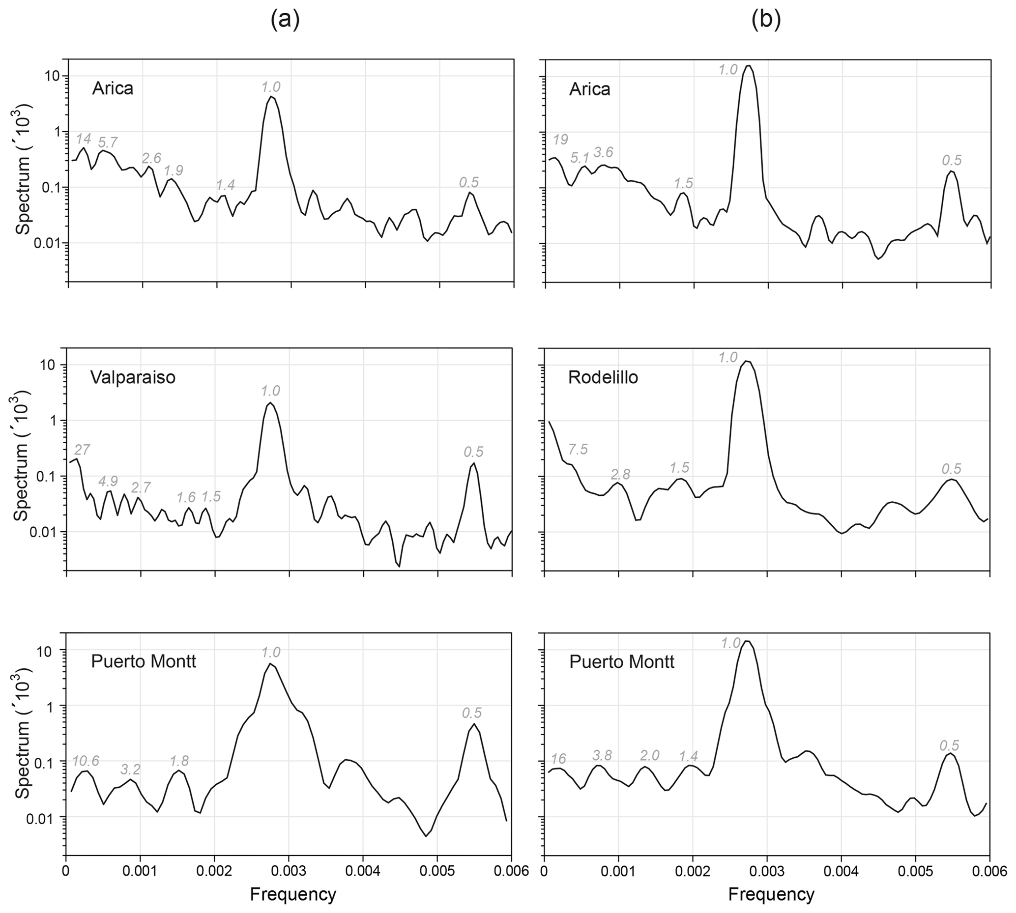
Figure 2Spectral analysis for three representative stations from the northern, central and southern regions of Chile. Column (a) corresponds to sea surface temperature time series (oceanic stations) and column (b) to atmospheric surface temperature time series (atmospheric stations). Dominant peaks are indicated together with their associated periods in years.
We carry out a univariate spectral analysis for the 16 stations. In Figure 2, we show the results for three atmospheric and three oceanic stations, which represent the northern, central and southern regions of Chile. The complete set of results is in Appendix B. The oceanic stations that show spectral peaks with the longest periodicities are Valparaíso with 27 years, Talcahuano with 20 years, Antofagasta with 18 years and Arica with 14 years. Four stations have periodicities with an intermediate value of 6 to 10.6 years. Three stations (Antofagasta, Valparaíso and Talcahuano) present a 4-year periodicity. Two stations have peaks around 3 years, and six stations present 2-year periods. In the eight stations, periodicities between 1.3 and 2 years were also found: most stations show periods of around 1.5 years.
The atmospheric stations that show spectral peaks with the longest periodicities are Antofagasta and Serena with 20 years, Arica with 19 years, Iquique with 18.8 years, Concepción with 16.4 years, and Puerto Montt with 16 years. Furthermore, Arica and Antofagasta share a periodicity of 5.1 years. There are three stations with periodicity around 4 years and five stations with periodicity around 3 years. Periodicities around 1.5 years were also found, as in the oceanic case. In general, longer periodicities can be observed for atmospheric surface temperature time series than for sea surface temperature. Possible causes of these periodicities can be found in the discussion in Sect. 4.1.
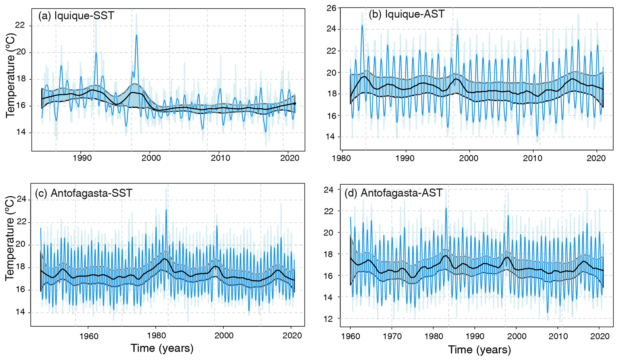
Figure 3Temperature time series of Antofagasta and Iquique. (a) Antofagasta sea surface temperature; (b) Antofagasta atmospheric surface temperature. (c) Iquique sea surface temperature; (d) Iquique atmospheric surface temperature. Interpolated original (light blue), trend cycle (blue) and long-term trend (black), together with confidence bands at 95 % (light blue).
We estimate the trend by means of the local polynomial smoother as detailed in Sect. 2.1.2. For the estimation of the long-term trend the degree of the polynomial was set to 1 to mitigate boundary effects; otherwise the order is 2. The confidence bands at the 95 % level for the nonparametric estimator of the trend were derived using an autoregressive wild bootstrap scheme, which is robust against the presence of missing data, serial dependence and heteroskedasticity. We show the results for Antofagasta (SST, AST) and Iquique (SST, AST) in Fig. 3. The estimated long-term trend for Antofagasta and Iquique might seem to indicate a tendency, but this is ruled out if we take into account the uncertainty (confidence bands in light blue). This suggests that the process that has generated the time series for both stations is mean-stationary, and this holds for all the stations. For more details, see Appendix B1.
Table 3Output from the best neural network fit from the grid search test for chaos of the time series of the oceanic stations. The table reports the embedding dimension d, the time delay τ, the number of hidden units k, the value of the minimized BIC, the global Lyapunov exponent (together with the value of the test statistic Z∗) and the p value of the test.
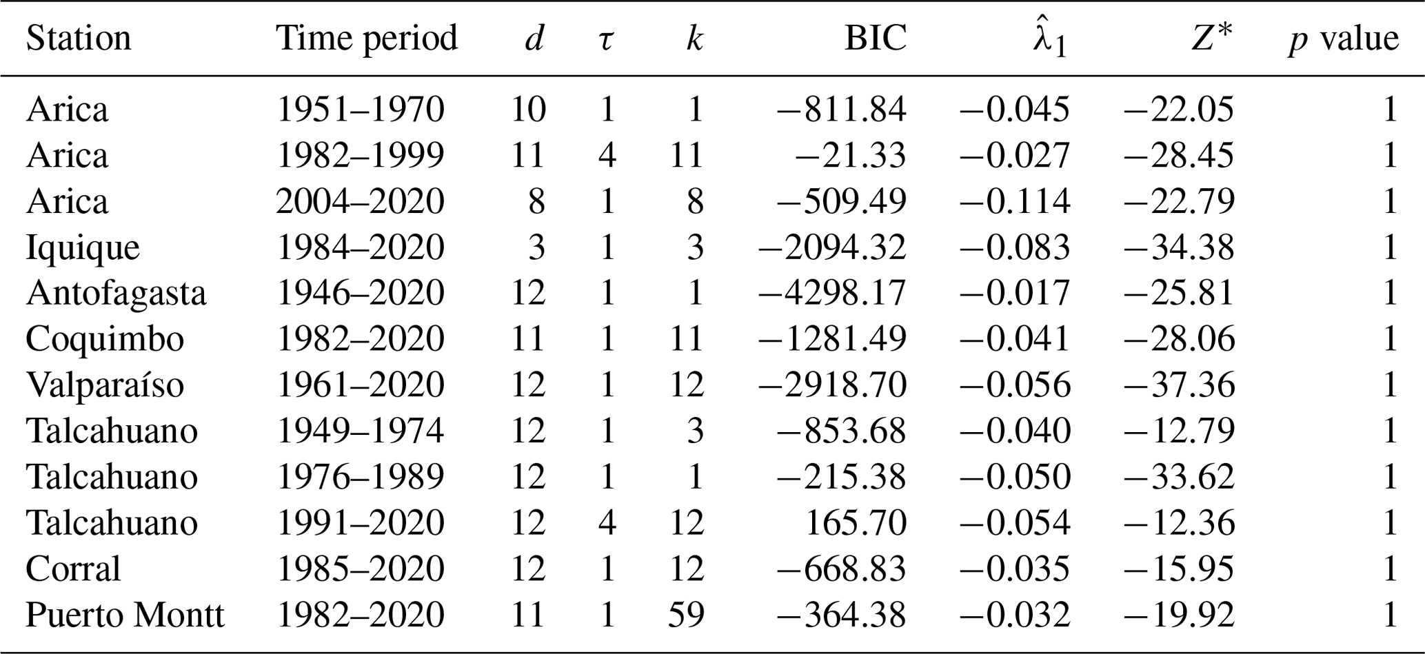
Table 4Output from the best neural network fit from the grid search test for chaos of the time series of the atmospheric stations. The table reports the embedding dimension d, the time delay τ, the number of hidden units k, the value of the minimized BIC, the global Lyapunov exponent (together with the value of the test statistic Z∗) and the p value of the test.
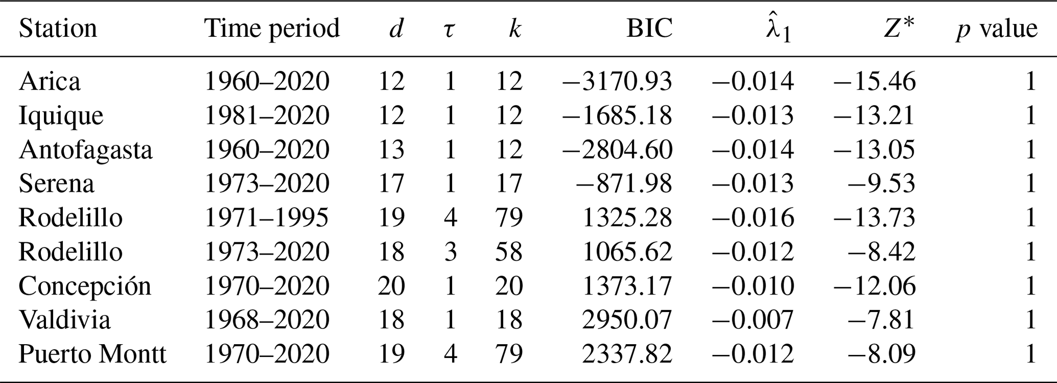
We estimate the largest Lyapunov exponent of the series and derive a rigorous (asymptotic) statistical test for chaos by following Shintani and Linton (2004). The approach is based upon a single-layer, feed-forward neural network model of the map and its Jacobian. More details on the procedure are reported in Sect. 2.2 and Appendix C. The null hypothesis of no chaos () is tested against the alternative hypothesis of a positive exponent (). One of the critical issues is the selection of the best neural network model, which we solve by means of the generalized Bayesian information criterion (BIC), where the global minimum is searched on a grid of embedding dimensions from d=3 to d=20 and time delays from τ=1 to τ=4. The results are presented in Tables 3 and 4 for the oceanic and atmospheric stations, respectively. Besides the station name and the time period, the tables report the values of the embedding dimension d, time delay τ and number of hidden units k of the network that produce the minimized BIC criterion over the parameter grid. The last two columns contain the value of the test statistic Z∗ and the p value of the test based on the asymptotic Gaussian null distribution, respectively. All the estimated exponents are negative and the test never rejects the null hypothesis of the absence of chaos for both the oceanic and the atmospheric stations.
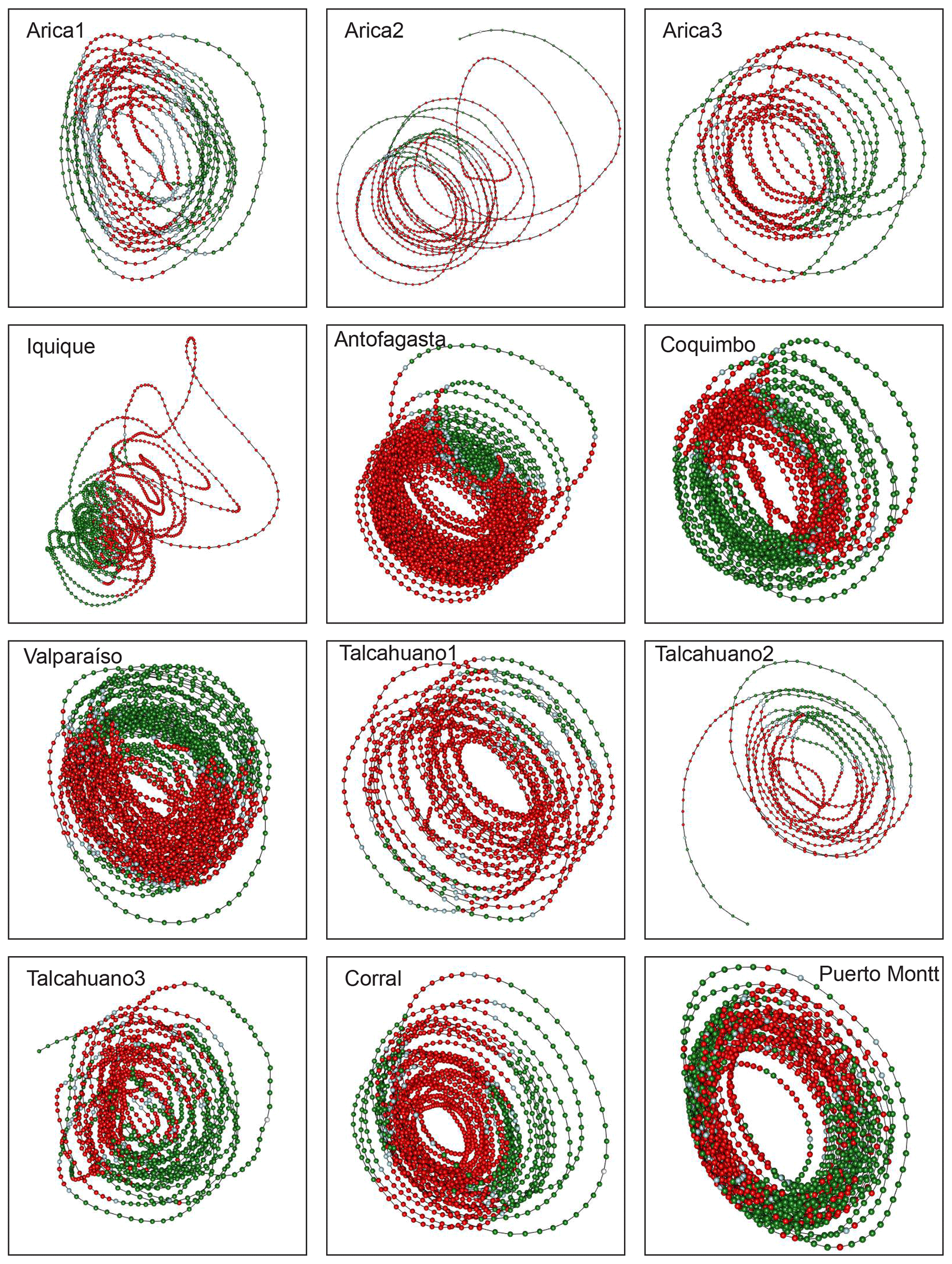
Figure 4Attractors for sea surface temperature with superimposed information on the local Lyapunov exponents. Red corresponds to a positive LLE, whereas green indicates a negative LLE. The subsections indicate the latitudinal order of the stations. In the case of Arica and Talcahuano there are three courts, which are numbered from 1 to 3. The temporal windows are 1 month for Iquique; 4 months for Arica; 5 months for Coquimbo, Valparaíso and Talcahuano; and 6 months for Antofagasta, Corral and Puerto Montt.
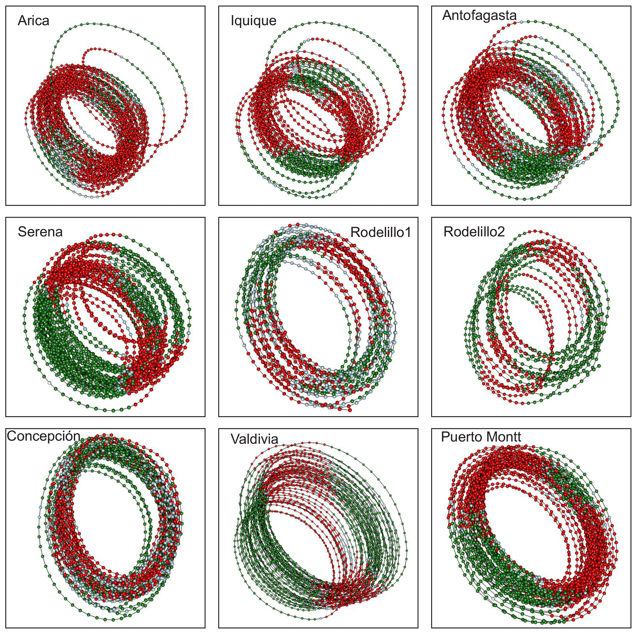
Figure 5Attractors for atmospheric surface temperature with superimposed information on the local Lyapunov exponents. Red corresponds to a positive LLE, whereas green indicates a negative LLE. The subsections indicate the latitudinal order of the stations. For the case of Rodelillo, there are two courts. The temporal windows are 5 months for Serena, Rodelillo, Concepción and Valdivia and 6 months for Arica, Iquique, Antofagasta and Puerto Montt.
This result is an important indication that the dynamics behind temperature in Chile is most probably nonlinear but not chaotic (Lorenz, 1963). We use local Lyapunov exponents (LLEs) to characterize local predictability throughout the stations. We varied the number of steps ahead, M, from 4 to 52 (i.e. from 1 month to 1 year) for oceanic stations and up to 260 steps ahead (5 years) for atmospheric stations. In order to uncover any association with El Niño, we chose three specific windows corresponding to the short (0 to 3 months), medium (6 to 9 months) and long term (12 to 22 months) and paid particular attention to the results obtained for the 1-, 6- and 12-month windows. In Figs. D1 to D3 of the Appendix we show the time series of the oceanic stations where the information on the 1-month, 6-month and 1-year LLEs, respectively, is superimposed: red corresponds to a positive LLE, whereas green indicates a negative LLE. The same information for the atmospheric stations is reported in Figs. D4 to D6. Likewise, in Figs. 4 and 5, we present the phase-space portraits of the attractors for the stations with superimposed information on the LLEs in red and green.
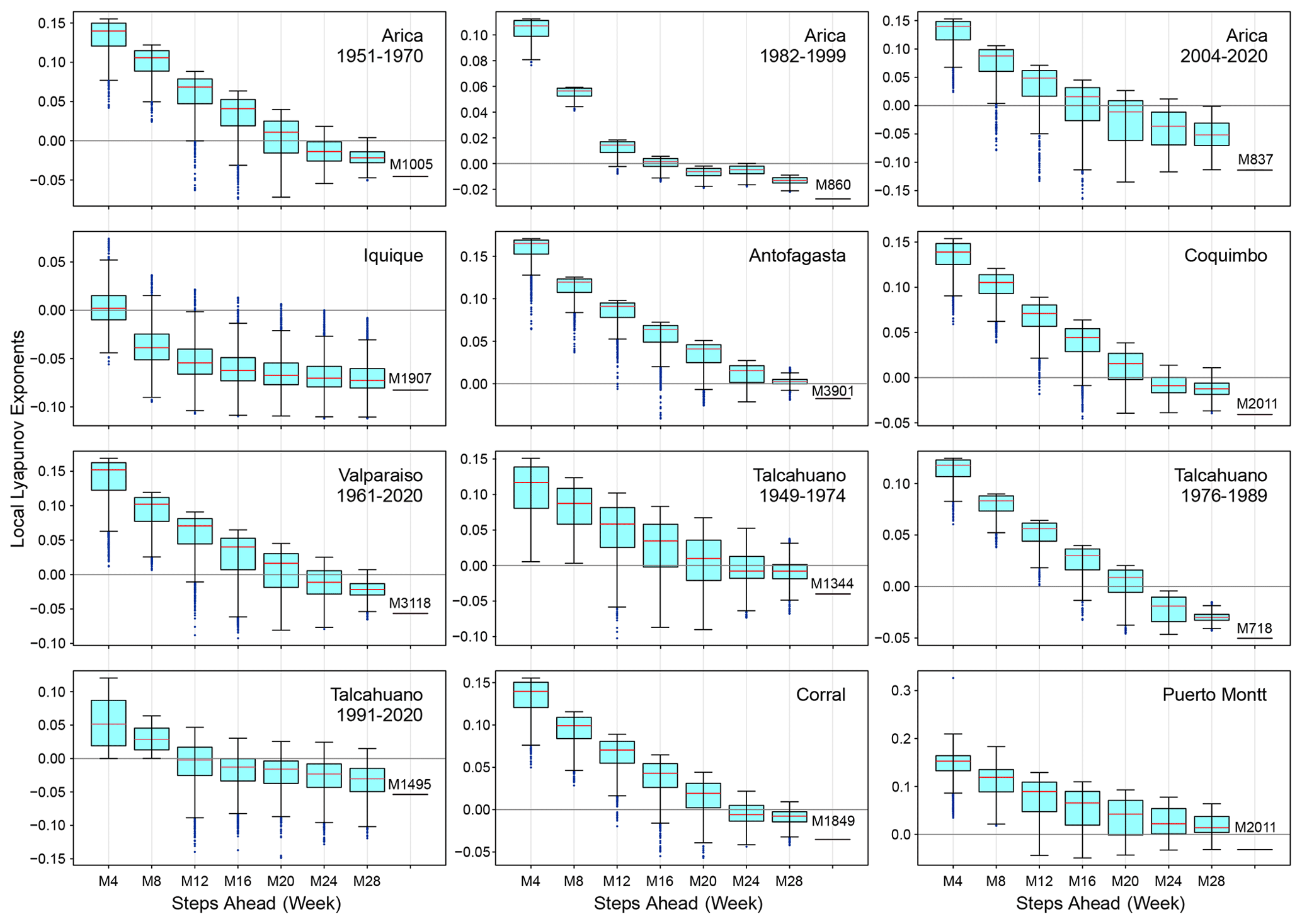
Figure 6Box plots of the local Lyapunov exponents versus steps ahead (M in weeks) for the sea surface temperature series. The series are arranged latitudinally.
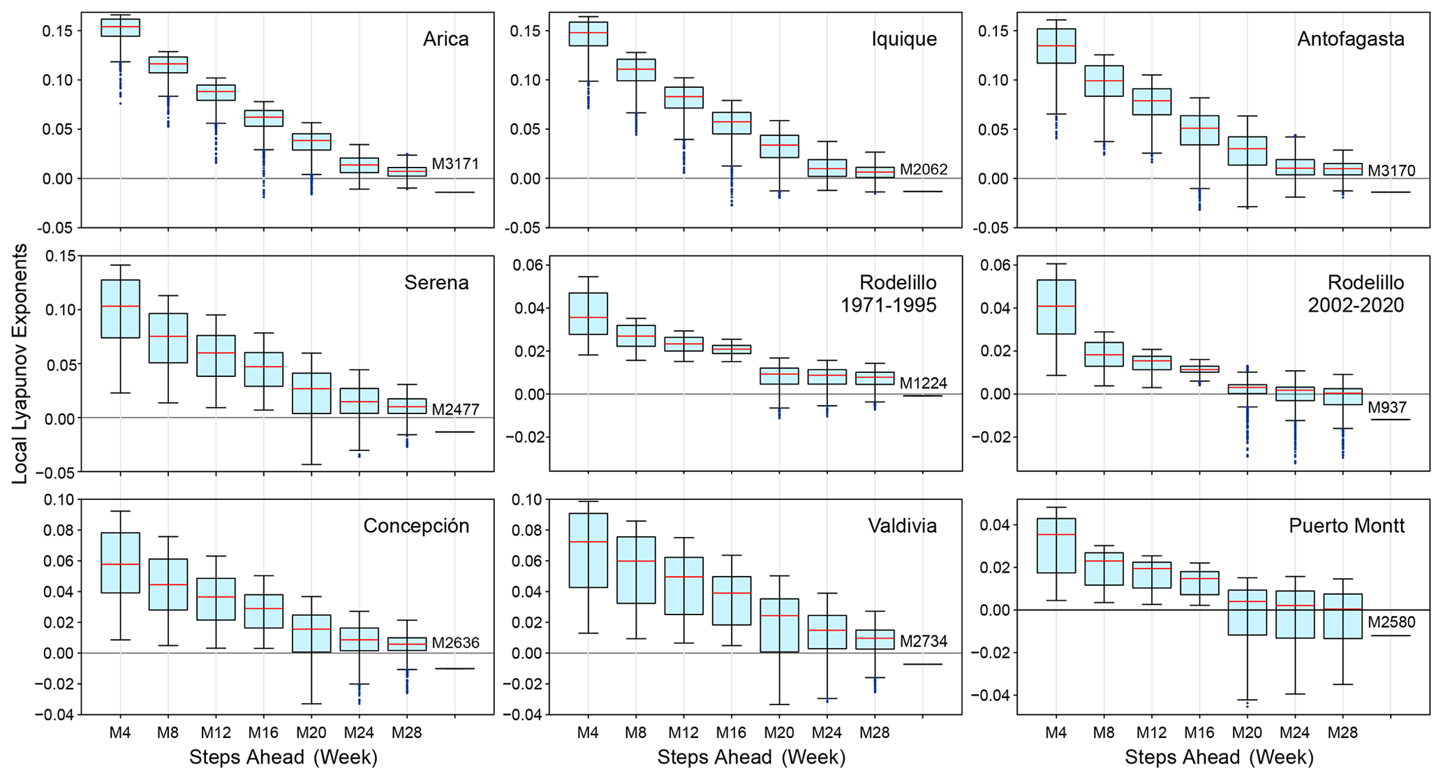
Figure 7Box plots of the local Lyapunov exponents versus steps ahead (M in weeks) for the atmospheric surface temperature series. The series are arranged latitudinally.
Comparing the LLEs of the oceanic stations with their atmospheric counterparts for the different windows, we found that for the 1-month window, both classes of stations showed unstable behaviour throughout the record, except for Iquique SST that shows patterns of both stability and instability. For the 6-month window in SST and AST, mixed stability and instability is observed, except for Iquique, where there is stability throughout the record. In the Antofagasta and Puerto Montt SSTs similar behaviour can be observed, showing instability at the extremes and stability in the middle part. Finally, for the 1-year window, all oceanic stations showed stability throughout the record, except for Talcahuano and Puerto Montt: that is, the southern region. Of the atmospheric stations, Arica, Iquique and Antofagasta showed instability in the extremes and stability in the middle part of the record; Rodelillo behaves totally stably, while Serena, Concepción and Valdivia present totally stable or unstable parts throughout the series. This is not the case for Puerto Montt, which presents very little instability. The box plots of the LLEs versus steps ahead (M) are shown in Figs. 6 and 7. Clearly, the sea surface temperature series approach the global exponent faster than the atmospheric series. For instance, for M=28 steps ahead, the box plots of the LLEs are already negative for all the SST series, with the exception of Puerto Montt (Fig. 6). On the contrary, for M=28 all AST time series still have positive LLEs (Fig. 7). Overall, the results indicate a qualitative difference in the temperature dynamics of the two types of series. This can be explained by considering that, on average, for the sea surface series but for the atmospheric series, so the latter are globally more stable. The presence of the ocean and its exchanges of heat and momentum with the atmosphere can easily reduce the instability properties of the atmospheric flow (Vannitsem et al., 2015).
In the following, we compare the information conveyed by local Lyapunov exponents with the Oceanic Niño Index (ONI). El Niño is characterized by a positive ONI greater than or equal to +0.5 ∘C. La Niña is characterized by a negative ONI less than or equal to −0.5 ∘C. To be classified as a fully fledged El Niño or La Niña episode, these thresholds must be exceeded for a period of at least five consecutive overlapping 3-month seasons. The Climate Prediction Center of the US National Oceanic and Atmospheric Administration (NOAA) considers El Niño or La Niña conditions to occur when the monthly Niño 3.4 SST departures meet or exceed ±0.5 ∘C along with consistent atmospheric features. These anomalies must also be forecast and should persist for 3 consecutive months. In the case of the oceanic stations, we note the following: in Antofagasta the expected behaviour is observed – that is, the whole series shows persistent instability for the 1- and 6-month windows throughout the record (Fig. D1c). This might be due to the warm water pool that is always found here simulating an El Niño. The same pattern is observed for the 1-year window, but, in this case, the behaviour is consistently stable (Fig. D3c). Arica shows instability throughout the record for the 1-month window, where instability decreases during El Niño events of 1953–1954, 1958–1959, 1963–1964, 1965–1966, 2009–2010 and 2014–2016 (Fig. D1a). During the 6-month and 1-year windows, it becomes more stable than unstable and shares the same behaviour with Talcahuano, where the third cut can be located lower than the other two and a very marked variability in the LLE can be seen (Figs. D2a, f and D3a, f). At these two stations the trajectory of the phase space for the second cut is interrupted (Fig. 4). In Talcahuano, interesting behaviour, with respect to the ONI, is only observed for the 1-month window, where the instability for the first cut for 1949–1974 decreases during El Niño events of 1953–1954, 1958–1959, 1963–1964, 1965–1966, 1968–1969 and 1972–1973, to show rising behaviour in the third cut of 1991–2020 during El Niño events of 1991–1992, 1994–1995, 1997–1998; 2002–2003, 2004–2005, 2009–2010 and 2015–2016 (Fig. D1f). In the case of Iquique, the 1-month and 1-year windows have stable and unstable behaviour; it is the only series in which the peaks of both the stable and unstable part coincide with several El Niño events of 1987–1988, 1991–1992, 1994–1995, 1997–1998, 2002–2003, 2004–2005, 2006–2007, 2009–2010, 2014–2016, 2018–2019 and 2019–2020 (Figs. D1b and D3b). For the 6-month window, the behaviour is stable throughout the record, but the stability peaks continue to coincide with the same El Niño events, with the exception of 2002–2003, 2004–2005, 2006–2007, 2018–2019 and 2019–2020 (Fig. D2b). Finally, Valparaíso, in the 1-month window, shows a decrease in the unstable part that corresponds to El Niño events of 1968–1969, 1972–1973, 1982–1983, 1997–1998 and 2014–2016 (Fig. D1e).
As concerns atmospheric stations, in Antofagasta the 1-month window shows unstable behaviour throughout the entire record and shows a temperature decrease during the 1972–1973, 1982–1983 and 1997–1998 El Niño events (see the highest temperature peaks in Fig. D4c). In the case of Arica, for the same window, a decrease in the unstable part is observed for the same El Niño events plus that of 2014–2016 (see the highest temperature peaks in Fig. D4a). Puerto Montt behaves in the same way as Antofagasta in its oceanic record: that is, it shows continuous unstable behaviour throughout the entire time span (Figs. D1h and D4h). The same occurs with Rodelillo for the 1-month window (Fig. D4e); its behaviour is similar to that of Antofagasta and Puerto Montt. Finally, for the 1-year window in Serena, instability increases from 1971 to 1982–1983, which is where it coincides with the El Niño event of that year. The behaviour decreases and increases again to coincide with El Niño of 1987–1988, and likewise, a peak of instability coincides with El Niño of 2014–2016 (Fig. D6d).
In summary, in the case of the oceanic stations, in Arica, Valparaíso and Talcahuano, the unstable part decreases significantly during various El Niño events, while for Antofagasta the behaviour is persistent throughout the record for both the stable and the unstable part; on the other hand, in Iquique the unstable behaviour increases during El Niño events and the stability decreases after them. For the atmospheric stations, it is in Arica, Iquique and Antofagasta where a decrease in instability during several El Niño events can be seen, contrary to what Serena shows with an increase in instability; only the latter shows this for the 1-year window, while the previous stations show an interesting behaviour of decrease for the 1-month window.
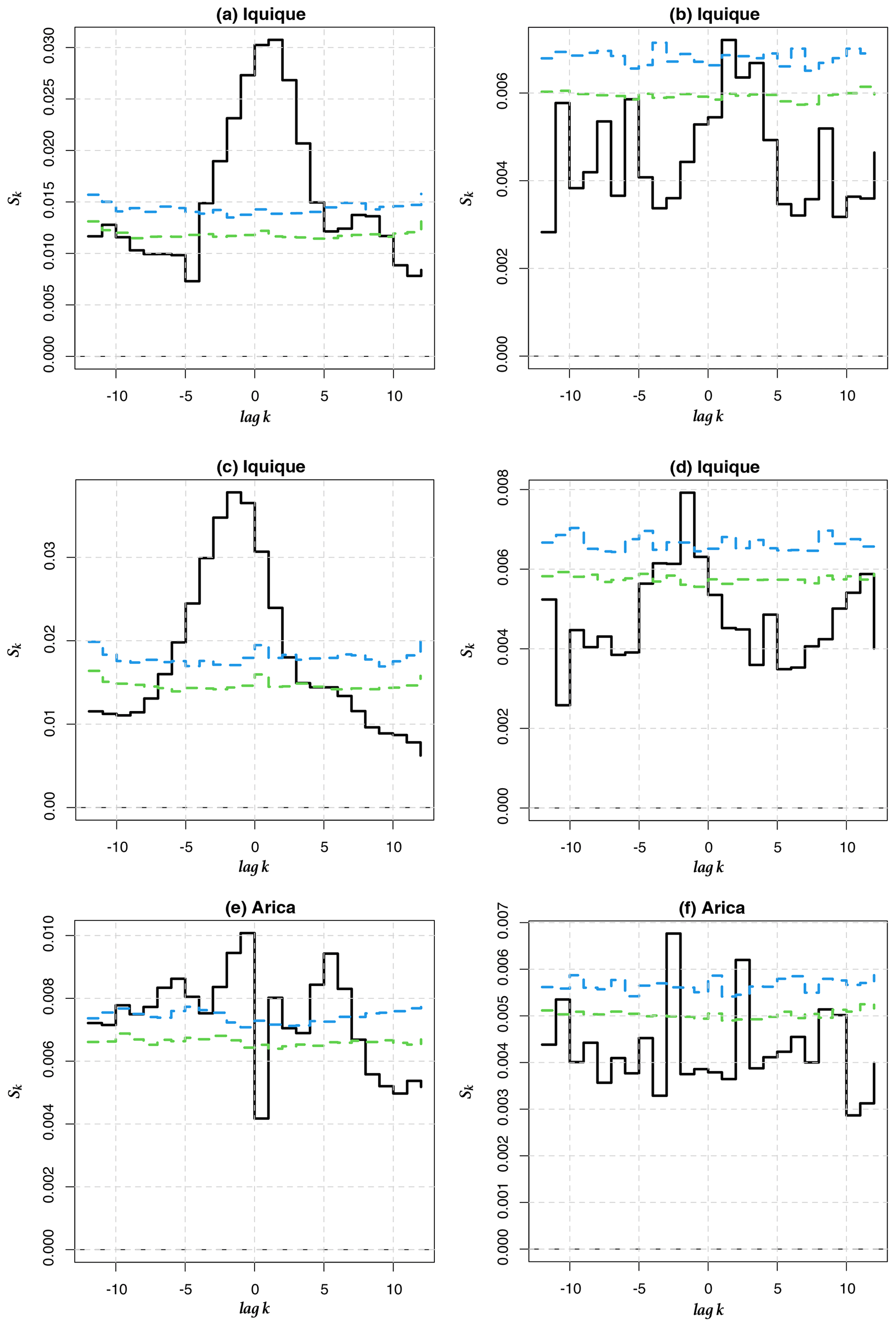
Figure 8Cross-entropy Sk for between the 1-month and 6-month LLEs (Iquique SST) and between the 1-month LLEs (Arica AST) and the ONI. (a, c, e) Original time series (b, d, f) pre-whitened time series. Iquique 1 month and 6 months correspond to the first two upper graphs and the two central ones, while Arica 1 month corresponds to the lower two graphs.
In order to go beyond this visual comparison and to corroborate whether there is a relationship between the ONI and the dynamics of climate variability in Chile seen through the LLEs, we compute the cross-entropy measure proposed in Giannerini et al. (2015) and Giannerini and Goracci (2023); see Appendix D. Rejection bands under the null hypothesis of cross-independence are derived through the moving block bootstrap, and the series have been pre-whitened using an autoregressive filter in order avoid spurious rejections due to serial dependence. The test was performed for all stations before and after pre-whitening. The most significant results are shown in Fig. 8, whereas the full set of results can be found in Appendix E. For Iquique SST, the cross-entropy test indicates a significant dependence at lag +1 and −2 with 1-month and 6-month LLEs, respectively. For the atmospheric stations, only Arica AST showed a significant dependence at lags +2 and −3. This implies that the ONI at time t is correlated with the LLE at times t+1, t−2, t+2 and t−3, respectively, for the aforementioned stations. For the 6-month time horizon, Corral also presents a significant dependence, which could be a false positive; see Fig. E4. We also applied the test to correlate the ONI and 1-year-ahead LLEs for Serena. The results in Fig. E7 do not show any significant cross-dependence. We offer a further discussion in Sect. 4.2.3 below.
4.1 Spectral analysis
The periods of 18, 18.8 and 19 years found for Antofagasta SST, Iquique AST and Arica AST could be linked to the PDO. They might also be associated with the lunar nodal cycle of 18.61 years, popularly known as “lunar wobble” – this low-frequency tidal cycle is due to the oscillation of the maximum lunar declination with respect to the Equator (Rossiter, 1962; Black et al., 2009) – since the variations of the lunar cycle influence the movement of ocean currents. The 4-year periods found in Antofagasta, Valparaíso and Talcahuano might be linked to the lunar perigee subharmonic of 4.4 years. The external forcing caused by the Moon is important, not only because of the changes caused in interannual timescales to the variability of the tidal range, but also because it influences the hydrodynamic energy of the ocean, altering sedimentation patterns (Oost et al., 1993; Gratiot et al., 2008) and coastal erosion (Smith et al., 2007), water level and coastal flood risk (Thompson et al., 2021), and ocean stratification (Devlin et al., 2017b, a, 2019).
Interannual periods can also be observed in the oceanic stations: 2.7 years for Iquique and Valparaíso, 2.6 for Arica, 2.5 for Coquimbo and Talcahuano, 2.4 for Antofagasta, 2.0 for Corral, and 1.8 for Puerto Montt. In the case of atmospheric stations, 2.7 years was found for Serena, 2.8 for Rodelillo, 2.3 for Valdivia and 2.0 for Puerto Montt. These periods could be related to the Quasi-Biennial Oscillation (QBO), a climatic alteration located in the Pacific Ocean that consists of zonally symmetrical easterly and westerly wind regimes that regularly alternate with a period that varies between 24 and 30 months and is manifested through hydroclimatological variables such as wind and temperature. Its eastern phases appear to be alternately related to the warm component of ENSO (Riveros et al., 2020). The QBO has already been seen in other records from the Chilean region between 39 and 43∘ S (Villalba et al., 1998). Fagel et al. (2008), when analysing layered sediments from Lake Peyuhue (40∘ S, 72∘ W), found that the frequency bands of the thickness of the layers were mainly related to QBO periodicities. In our case, we found this oscillation in oceanic and atmospheric surface temperature records. For the oceanic records it was found in all the stations, something that did not happen with the atmospheric records, where it is only seen for the stations in the central and southern parts of Chile. Similarly, periods related to ENSO and PDO were obtained, as well as some others that we believe may be related to local events; however, it should be noted that QBO has also been related to ENSO.
Regarding the periodicity of 1.5 years found in both classes of station, Jiang et al. (2020) have noted this periodicity in modes of tropical Pacific surface wind anomalies, also referred to as the so-called combination mode (C-mode). This C-mode emerges from nonlinear interactions between the warm pool annual cycle and ENSO variability (Stuecker et al., 2013). Sakova et al. (2006) likewise found an 18-month signal in altimeter sea surface height over the whole Indian Ocean, which they associate with Indian Ocean dipole events, similar to ENSO, and statistically linked to it (Stuecker et al., 2017), but taking place in the equatorial Indian Ocean.
4.2 Nonlinear analysis and ONI
The effects of changes in the SST and AST on biota range from the redistribution of species (Lubchenco et al., 1993; Ihlow et al., 2015), the increase in vulnerability that occurs in the HCS due to the expansion of oxygen minima associated with the increase in SST (Mayol et al., 2012; Stramma et al., 2008), and increases in extreme events (Harris et al., 2018; Garreaud, 2018) to subtle changes in biological–climatic feedbacks (Bradford et al., 2019; Bardgett et al., 2008), all of which invite discussions about the contribution of the oceans to these feedbacks (Joos, 2015). For these reasons, understanding the effects of climate variabilities such as El Niño on the behaviour of long time series of coastal temperature records can contribute to improving forecasts and understanding the effects of climate change and climate variability in systems such as the HCS (Harris et al., 2018). The results consistently indicate the presence of nonlinear, non-chaotic oscillators for both oceanic and atmospheric stations. LLE analysis highlights patterns of reduced and enhanced stability and predictability in the phase space, where the asymptotic behaviour of the LLEs towards the negative global Lyapunov exponent differs in oceanic versus atmospheric stations, since stability is reached faster in oceanic stations, where the oceanic environment is less perturbable than the atmosphere due to the great heat capacity of water.
4.2.1 Oceanic stations
For both oceanic and atmospheric stations, Antofagasta shows the slowest speed of convergence in the oceanic case, accompanied by Corral. Antofagasta is characterized by the constant presence of warm water inside its bay (Piñones et al., 2007), so its climate possesses a type of local permanent El Niño, keeping the bay in a state of external forcing. This makes the dynamics of the Antofagasta system look unstable in the LLEs, and when comparing with ONI it is not possible to distinguish different behaviour when a general El Niño event occurs. Regarding Corral, there is a cooling trend in the coastal upwelling regime along northern Chile and southern Peru, which contrasts with the warming trend in the last 350 years in an offshore area of the Humboldt Current System at 36∘ S (Vargas et al., 2007). Such El Niño-type conditions also found in Corral might explain its reduced speed of convergence. The case of Iquique SST is peculiar not only due to its attractor, which shows an abrupt change, but also because of the estimated embedding dimension (d=3) that is much lower than that of the other stations, with mixed dynamics for the window of 1 month and a positive cross-dependence between the ONI and the LLE. This indicates a strong relationship between the climate variability of this region and the El Niño phenomenon. Fuenzalida (1985), through an analysis of El Niño 1982–1983, showed that an increase in temperature in Iquique is associated with this phenomenon. In our case, the cross-dependence test showed a significant correlation at lag +1 for the 1-month LLEs and at lag −2 for the 6-month LLEs. The difference between the two is that the record observed at 1 month presents stabilities and instabilities, which, together with other factors discussed below, favour a leading effect and could be associated with the warm phase of ENSO. As for the 6-month LLEs, the behaviour of the area is completely stable; perhaps for this reason there is a lagging effect associated with the cold phase of ENSO. Notably, like La Serena and Valdivia, with similar dynamics occurring between them as discussed below, Iquique is also in a transition zone, the faunal transition zone, located south of the subtropical and north of the subantarctic zone (Bé and Tolderlund, 1971). In addition, the northern part of Chile, in which Iquique is located, is an area with wind-driven coastal upwelling throughout the year. Barbieri et al. (1995) analysed the northern region and found four sources of upwelling in Iquique. The upwelling south of Iquique is the most important due to its latitudinal extension. For this area the highest correlation between wind and SST is observed. Due to the peculiar oceanic and environmental characteristics of the Iquique area, we can hypothesize that the abrupt change observed in the trajectory of the SST transition could be due to the climate of 1976–1977, which, according to Namias (1978), Houghton et al. (2001) and Solomon et al. (2007), was a coupled global variation of the atmosphere–ocean system that links the variability of the sea surface temperature of the Pacific and climatic parameters in most of the world. Although this was a global variation, this abrupt trajectory change is present in Iquique, in contrast to the other stations, where the shape of the attractors indicates the presence of nonlinear oscillators, possibly forced. Likely, these peculiar features associate Iquique's dynamics with ENSO events. Also, we found similarity between the dynamics of Arica – upwelling throughout the year – and Talcahuano – seasonal upwelling. This could be the result of large-scale oceanic processes that occur simultaneously in both places. In Castro et al. (2020), similar variations of δ13C of particulate organic matter were noted in Iquique and Talcahuano, despite being two totally different areas; this was hypothesized to be influenced by coastal outcrop. In our case, since Arica is not very far from Iquique, we can think of this outcrop as part of the explanation for the similarity of the dynamics that we found. On the other hand, we have the northward currents that carry subantarctic water, as well as the intrusion of subtropical waters to the south, which during El Niño conditions can approach the coastal zone, causing the propagation of trapped waves to the coast and a poleward subsurface flow. From a dynamical point of view, this variability can affect currents, the mixing of the water column, the intensity of upwelling, and the temperature and sea level on the continental shelf and slope throughout the Humboldt Current System (Shaffer et al., 1997, 1999). In addition to this, the Chilean continental shelf is extremely narrow compared to the Atlantic coast, with a maximum width close to 45 km in the Talcahuano area and a general maximum depth of 150 m, except for the Valparaíso area, where it reaches up to 800 m (Camus, 2001). So, these may be other possible explanations for the similarity in dynamics found in these two regions. However, something else must be happening between the two stations to maintain this dynamics in the three study windows.
4.2.2 Atmospheric stations
Rodelillo, Puerto Montt and Antofagasta ASTs present similarities with Antofagasta SST. The former three stations present persistent behaviour throughout the time span for both northern and southern regions of Chile. Therefore, we can infer the presence of teleconnection processes throughout the zone. Gómez (2008) made hydrographic and meteorological observations during the period 1996–2005, finding an interannual and decadal modulation of the beginning of the upwelling season during the period 1968–2005 for the central–southern zone of Chile. This modulation would be linked to changes in atmospheric circulation patterns, associated with teleconnections triggered during El Niño. According to this study, the presence of teleconnections in oceanographic processes is needed. Finally, for the atmospheric stations of Arica, Iquique and Antofagasta, a decrease in unstable behaviour can be seen during El Niño events, possibly due to the effects of the Pacific anticyclone. Regarding Arica, the cross-entropy test showed a significant cross-dependence between ENSO and 1-month LLEs at lags +2 and −3. Puerto Montt is the southernmost station on the northern border of Patagonia (Garreaud et al., 2013). This station is located well inside the continent, on the coast of an inland sea, with greater thermal amplitudes due to the continental effect. As this station is located south of the southern limit recognized for the influence of El Niño, it is possible that El Niño is not responsible for the climate variability at this station, but rather the Southern Annual Mode (SAM) (González-Reyes, 2013), since we can also see unstable dynamics in the oceanic part (Puerto Montt SST). However, for this region there is already a high degree of disturbance, so what could be happening here are further intensifications induced by El Niño. This may be the reason why a behaviour similar to that of Antofagasta SST is also observed when we compare the ONI and the LLE AST of both stations.
In the case of Rodelillo, we can hypothesize that the local climate is greatly influencing the results obtained; this series was divided into two parts, which showed homogeneous results for the three different types of windows: that is, if the first segment of Rodelillo for the 1-year window was stable, the second was, too. This area is in the central zone of Chile and most of the wildfire activity in the country (Soto et al., 2015; Urrutia-Jalabert et al., 2018) is concentrated in both the central and central–southern zones of Chile (32–43∘ S), where ENSO and the Antarctic Oscillation (AAO) have a significant influence (Urrutia-Jalabert et al., 2018). This may be what maintains homogeneous results in Rodelillo's dynamics.
For their part, La Serena and Valdivia show similar dynamics for the 6-month windows. La Serena, in a transition zone between the hyperarid northern Atacama Desert and the more mesic Mediterranean region of southern central Chile, is strongly affected by ENSO, which is the primary driver underlying the high interannual variability in precipitation, and which promotes higher average rainfall during the warm phase (Rutllant and Fuenzalida, 1991). On the other hand, Valdivia is located within a transitional area between the influence of ENSO and SAM. The dynamics of both seasons is influenced by ENSO; however, the effect of the tropical South Pacific anticyclone also plays an important role in this similarity, as the effects of this semi-permanent high-pressure system change from 35∘ S, 90∘ W in January to 25∘ S, 90∘ W in July (Kalthoff et al., 2002; Montecinos et al., 2015): that is, in a period of 6 months, which is one of the windows that we use and in which important changes in the dynamics of the systems can be seen. The influence of the anticyclone is permanent to the north of 30∘ S, maintaining dry conditions, and weak south of 40∘ S (Camus, 2001), where there is rain throughout the year, which is why it has important effects in Valdivia. For La Serena, the cross-entropy test did not show significance; Fig. E7. This indicates that, although the instability of the dynamics in Serena is influenced by ENSO, it is not this phenomenon that contributes the most to the instabilities. We found similar results for Valdivia. This was expected because this area is also influenced by SAM and it is likely that the latter has a greater influence on the area.
4.2.3 ONI
Of all the oceanic stations tested, only Iquique SST (1- and 6-month LLEs) showed a significant cross-dependence with ENSO. In the case of atmospheric stations, only Arica AST (1-month LLEs) showed a significant cross-dependence with ENSO. This indicates that the association between LLEs and ENSO only occurs in the northern part of Chile. A possible explanation for this may be the disturbances coming from the Equator that only influence the northern part of Chile and that can affect the physical environment (Pizarro et al., 1994). On the other hand, the correlations obtained with a forward or backward lag could be related to the initial conditions that influence the westerly winds, since, according to Fedorov (2002) and Fedorov et al. (2003), during the beginning of a warm event, a westerly wind can accelerate the development of the event, while one after the peak of El Niño will simply prolong its duration. The majority of the published studies on ENSO in Chile report findings for the northern and central regions (Gutiérrez and Meserve, 2003; Holmgren et al., 2001; Guera and Portflitt, 1991; Vilina et al., 2002; Ulloa et al., 2001; Acosta-Jamett et al., 2016); although ENSO is a phenomenon that affects the climate globally, it has a greater influence on the northern part of our study region. Each El Niño event it is likely to affect the various areas of the Chilean region differently. This can be seen in Barbieri et al. (1995), who observed that during the 1987 El Niño the mean SST showed values above 1.5 ∘C throughout the year, while during the 1992 El Niño these anomalies occurred from March to May and from September to November. It is a fact that El Niño influences the regional climate, as do the PDO and the SAM.
We examined with an LLE analysis the patterns of local instability for the 16 stations, and these correlate on some occasions with ENSO events. However, it is only for the northern stations, specifically Iquique SST and Arica AST, that a significant correlation can be observed. ENSO, despite being a phenomenon that affects the climate globally, has greater influence in the northern part of Chile.
Teleconnections are noted throughout the entire region that may be associated with ENSO, PDO, SAM, the Pacific anticyclone, upwelling zones, QBO and the C-mode. A link can be seen between the climate variability of the region and different internal forcings (PDO, ENSO, SAM, C-mode and Pacific anticyclone) and external ones (QBO, lunar cycle) that contribute to the complexity of the system and favour a change in the variability as we move in latitude, which is due, in part, to the fact that it is necessary to take regional characteristics into account if one wants to understand the response of the different studied systems, oceanic and atmospheric, to the different forcings.
Previously unused Chilean naval temperature data from a large latitudinal spread of stations have helped us to uncover a great variety of factors involved in the temperature dynamics of the Chilean region. We find a non-chaotic climate variability, but with a nonlinear behaviour, reinforcing what has been mentioned in the literature. Our study invites more detailed work on the northern part of Chile, especially on Iquique and its sea surface temperature, where the behaviour of the system was very peculiar in both its low embedding dimension and the shape of the attractor as well as the significant correlation with ENSO for time horizons of 1 and 6 months.
The Humboldt Current System (HCS) that brings water from the tropical and sub-polar regions is characterized by evident interannual and seasonal variabilities (Mayol et al., 2012). The system is composed of (i) the Humboldt Current predominantly away from the equatorial coast that moves at an average surface velocity of 6 cm s−1, (ii) coastal currents formed by the Peru–Chile current and countercurrent, and (iii) the Peru–Chile equatorial coastal current. The currents towards the pole are responsible for transporting equatorial and subtropical subsurface waters to the Chilean coasts, while the flow towards the Equator brings cold Antarctic and Antarctic intermediate waters. The HCS is controlled to a large extent by the equatorial coastal winds linked to the Pacific subtropical anticyclone, which promotes the coastal upwelling associated with the primary productivity in the north and centre of Chile, extending its influence to the south of Chile in summer (Montecino et al., 2006). Around the western tropical zone of the Pacific there are ocean–atmosphere interactions that have effects at the planetary level (Enfield and Allen, 1980). In particular there is the El Niño–Southern Oscillation (ENSO) phenomenon, characterized by two opposite phases: one of warming and rainfall in the eastern Pacific, known as El Niño, and a second of cooling and dry years called La Niña (Pizarro and Montecinos, 2004). The redistribution of temperature in the water column can be associated with the passage of low-frequency coastal trapped waves (CTWs) (days at the intra-seasonal scale) and cool and warm interannual anomalies produced by equatorial waves due to the Southern Oscillation of El Niño (Shaffer et al., 1997; Montecinos and Gomez, 2010). In addition to ENSO, there is the Pacific Decadal Oscillation (PDO), which develops in the northern Pacific Ocean. It may be described as a long-period ENSO (Núñez et al., 2013), since it also has a positive or warm phase and a negative or cold phase but a different timescale. The PDO can intensify or diminish the impact of ENSO, depending on the relative phase in which these two oscillations are found. When ENOS and PDO are in phase, the impacts induced by El Niño or La Niña will be magnified with respect to normal patterns. Conversely, if ENSO and PDO are in opposite phases, the effects on global climate variability will be weaker (Wang et al., 2014). The Southern Annual Mode (SAM) or Antarctic Oscillation defines the changes in the westerly winds that are driven by atmospheric pressure contrasts, which in turn generate pressure differences between the tropics and the southern polar areas. The change in position of the western wind band, produced from west to east in latitudes between 30 and 60∘ of both hemispheres, influences the strength and position of cold fronts and midlatitude storm systems. In the positive phases of SAM, a belt of strong westerly winds contracts towards Antarctica. This results in weaker than normal westerly winds and high pressures in southern Australia, restricting the entry of colds fronts. SAM differentially affects the surface temperature of the four continental masses of the Southern Hemisphere, including part of the area influenced by the HCS at midlatitudes (Gillett et al., 2006). In conjunction with ENSO, SAM also partially explains the coastal temperature anomalies at high latitudes (Fogt and Bromwich, 2006) and also at midlatitudes (Yeo and Kim, 1992).
Figures B1 and B2 show spectral analyses performed for the oceanic and atmospheric stations. Numbers are given for the spectral peaks with the highest energies.
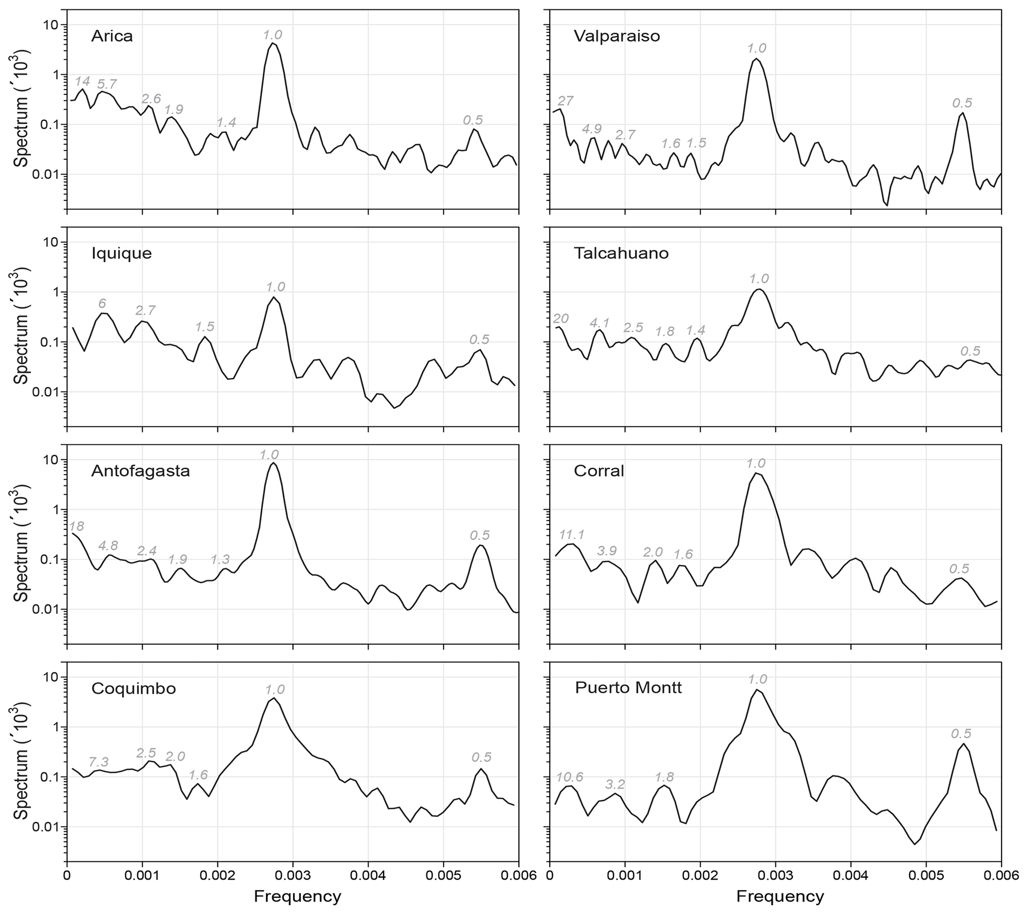
Figure B1Spectral analyses for oceanic stations. The numbers indicate the spectral peaks with the highest energy.
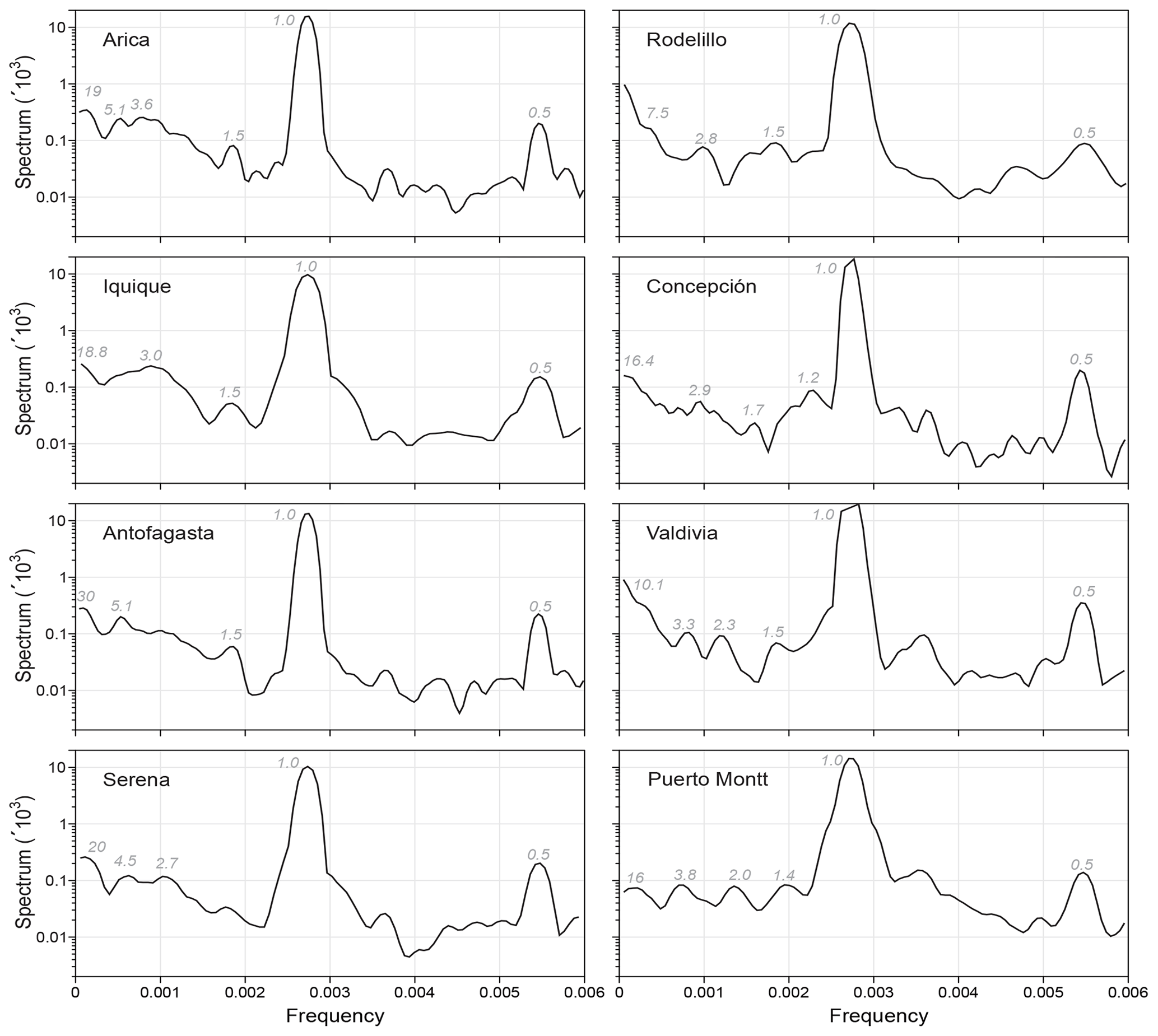
Figure B2Spectral analyses for atmospheric stations. The numbers indicate the spectral peaks with the highest energy.
B1 Trend estimation
In Figures B3 and B4 trend estimations are given for the 16 stations in a latitudinal manner from north to south.
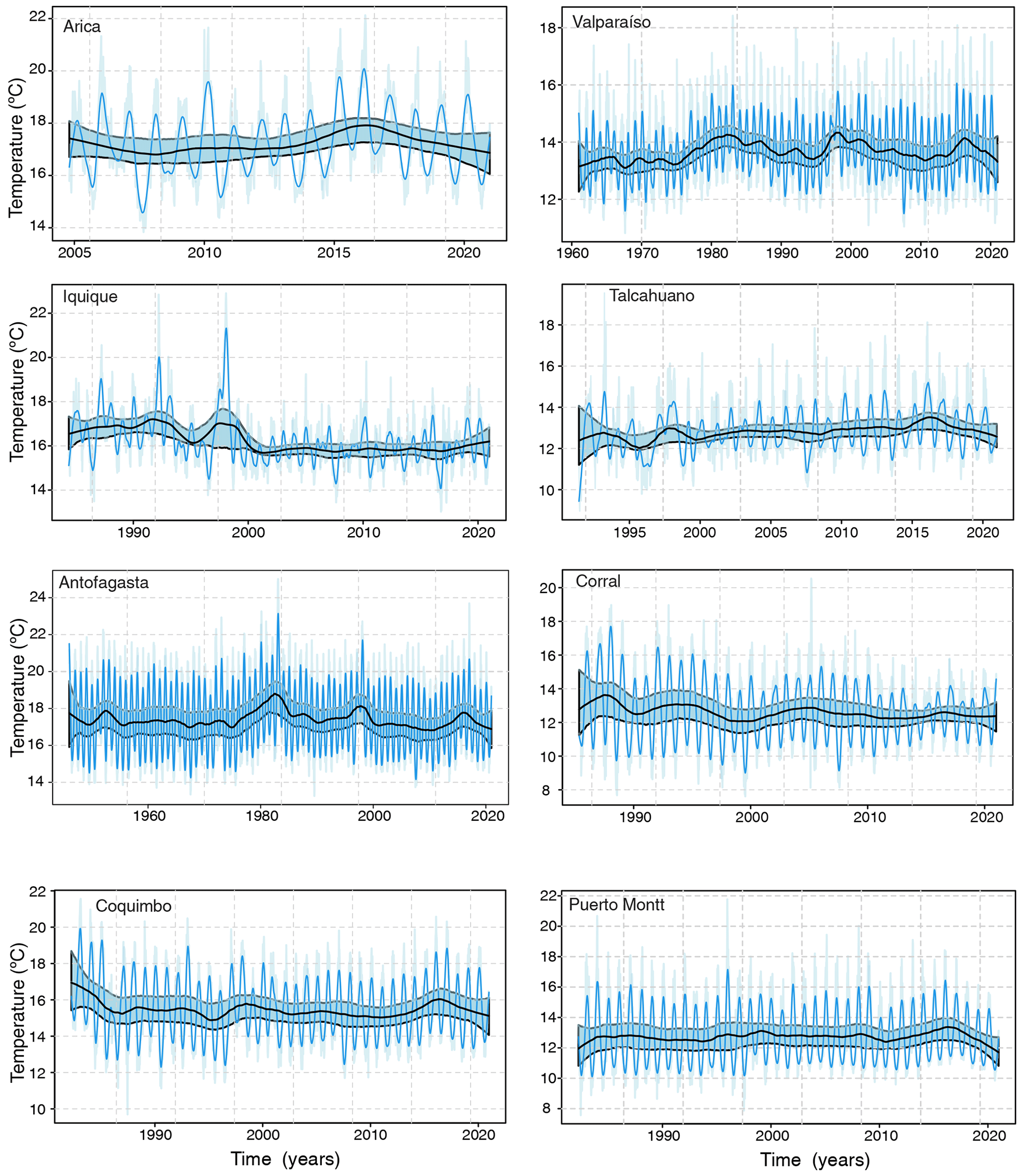
Figure B3Trend estimation for oceanic stations. Interpolated original (light blue), trend cycle (blue) and long-term trend (black), together with confidence bands at 95 % (light blue).
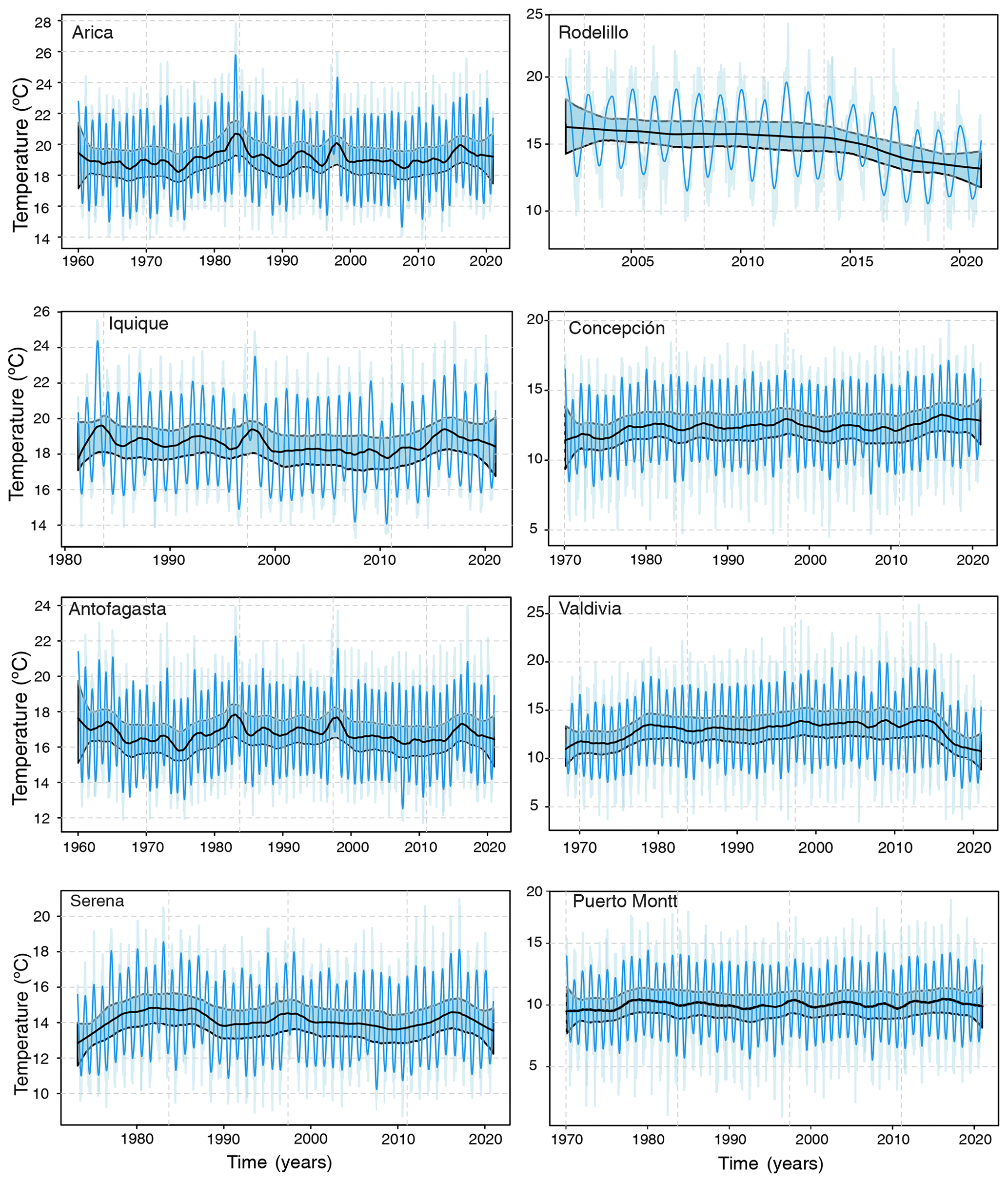
Figure B4Trend estimation for atmospheric stations. Interpolated original (light blue), trend cycle (blue) and long-term trend (black), together with confidence bands at 95 % (light blue).
As in Sect. 2.2, the dynamical system has the following representation:
where Et is an error process in ℝd. We assume that the data {Xt} are generated by the nonlinear autoregressive model
where Xt∈ℝ and {εt} is a sequence of independent random variables with E(εt)=0 and Var(εt)=σ2. Also, we denote with Jt the Jacobian of the map, evaluated at Xt. The model of Eq. (C1) can be seen as the state-space representation of the system of Eq. (C2), where and . We derive a consistent estimator for the map F and its Jacobian through a neural network estimator of fd. Neural networks are a class of nonlinear models inspired by the neural architecture of the brain (Nychka et al., 1992). These are made up of layers that in turn have connected “neurons”, which send messages and share information with each other. Layers are classified into three groups: (1) input, (2) hidden and (3) output. The input values Xt are received by the input units, which simply pass the input forward to the hidden units uj. Each connection (indicated by an arrow) performs a linear transformation determined by the connection strength ωij so that the total input to unit uj is
and each unit performs a nonlinear transformation on its total input:
The activation function ψ is a sigmoidal function with limiting values 0 and 1 as x→ −∞ and + ∞, respectively. Here we use
Other choices of the activation function are possible even if it does not have a major impact upon the final output. The hidden layer outputs uj are passed along to the single output unit, which performs an affine transformation on its total input. Therefore, the network output fd, for d inputs and k units in the hidden layer, can be represented as
We made use of the R nnet package to implement the estimator, and we used least-squares minimization (Venables and Ripley, 2002). We also experimented with conditional maximum likelihood without noticing major discrepancies in the results. The major challenge in regression with neural network models is selecting among the many possible combinations of d and k. Here we choose the best model that minimizes the BIC defined as
where the error variance is estimated through the residual sum of squares . Once the estimator is obtained, a consistent estimator for the map F and its Jacobian J can be derived with plug-in methods, as described in Shintani and Linton (2004).
In Figures D1 to D6 local Lyapunov exponents are shown for all 16 stations for 1-month, 6-month and 1-year windows.
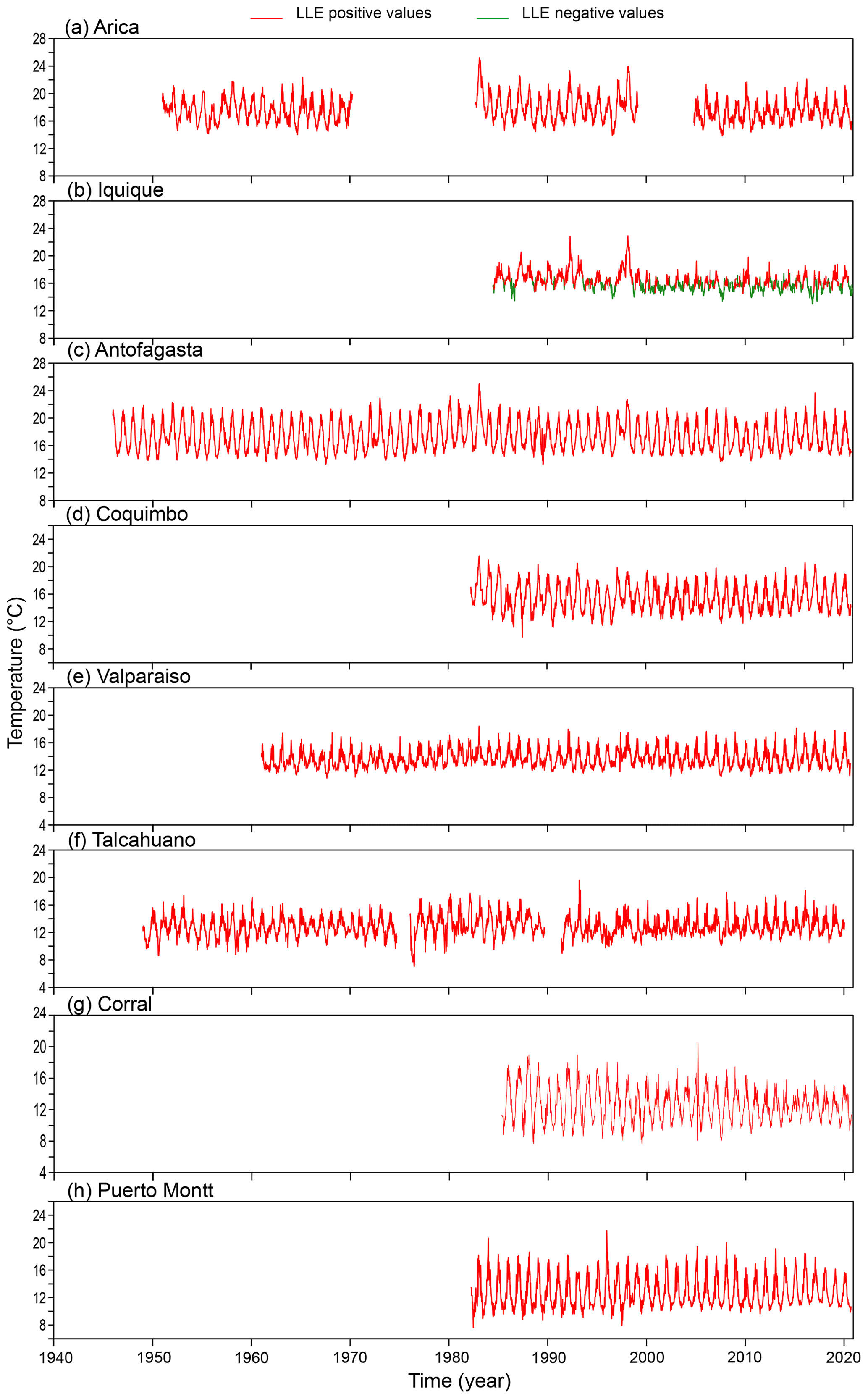
Figure D1Temperature record for ocean stations with superimposed information on 1-month local Lyapunov exponents: positive values for the LLEs are shown in red, and negative values are shown in green. Stations are given in a latitudinal arrangement.
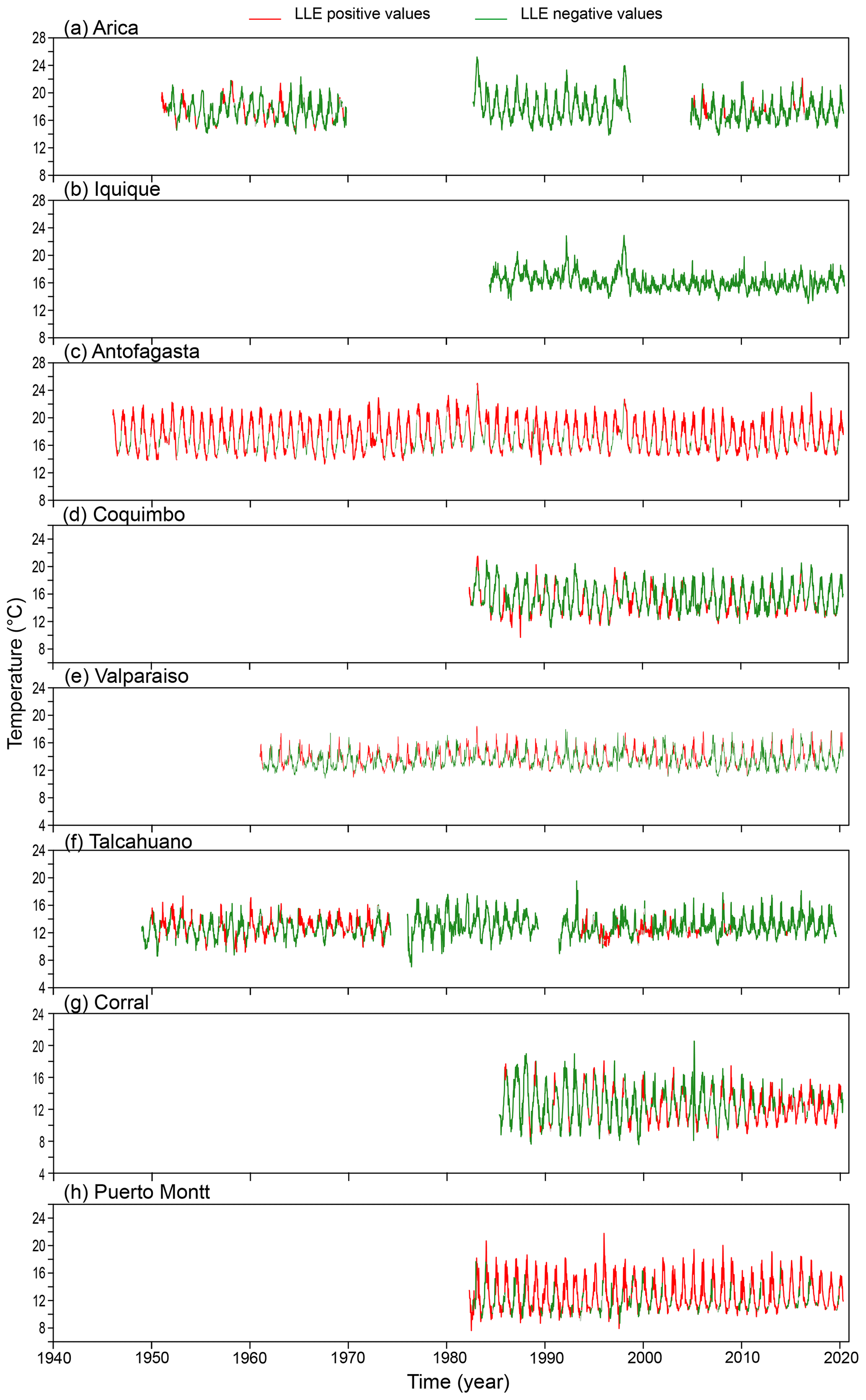
Figure D2Temperature record for ocean stations with superimposed information on 6-month local Lyapunov exponents: positive values for the LLEs are shown in red, and negative values are shown in green. Stations are given in a latitudinal arrangement.
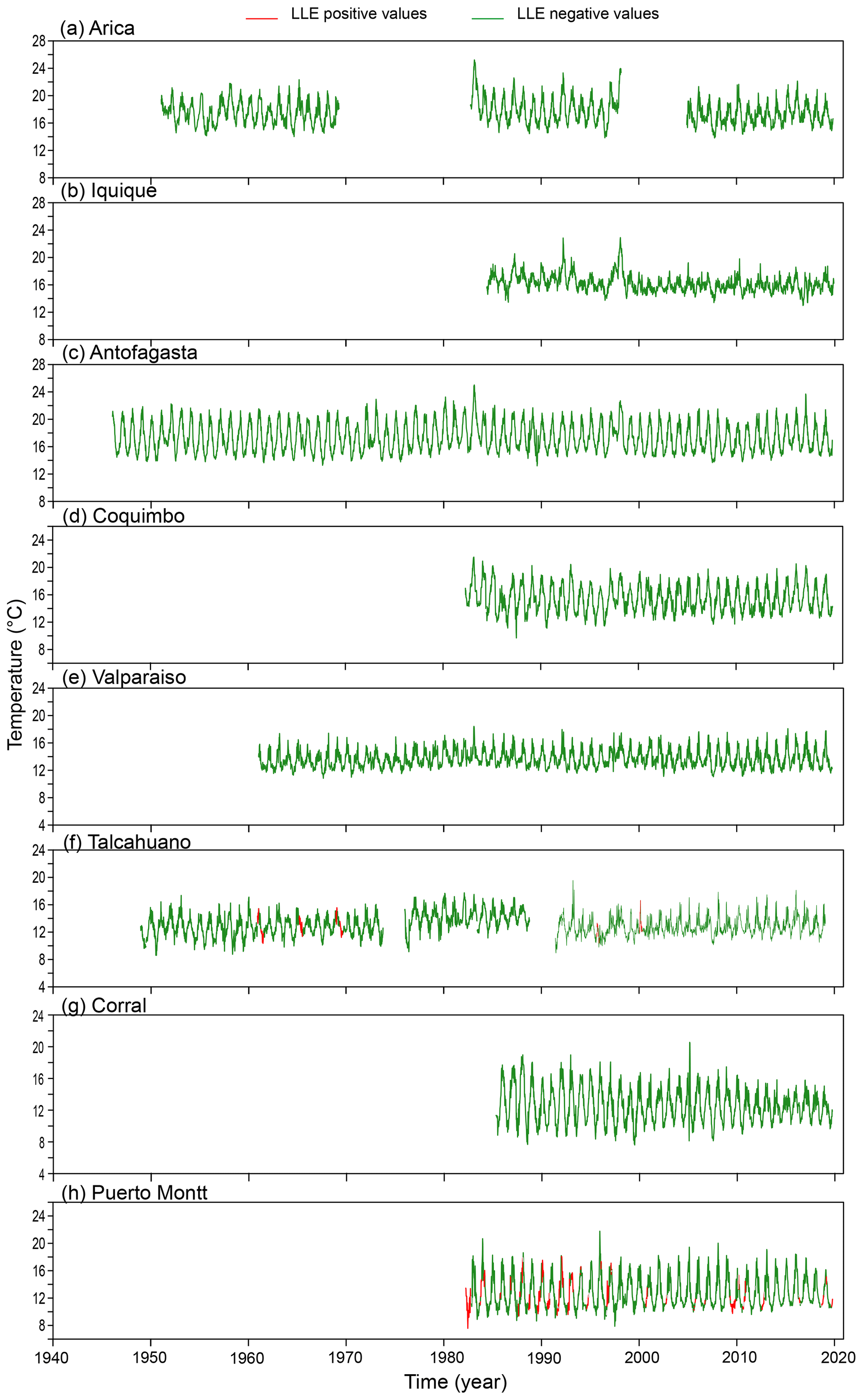
Figure D3Temperature record for ocean stations with superimposed information on 1-year local Lyapunov exponents: positive values for the LLEs are shown in red, and negative values are shown in green. Stations are given in a latitudinal arrangement.
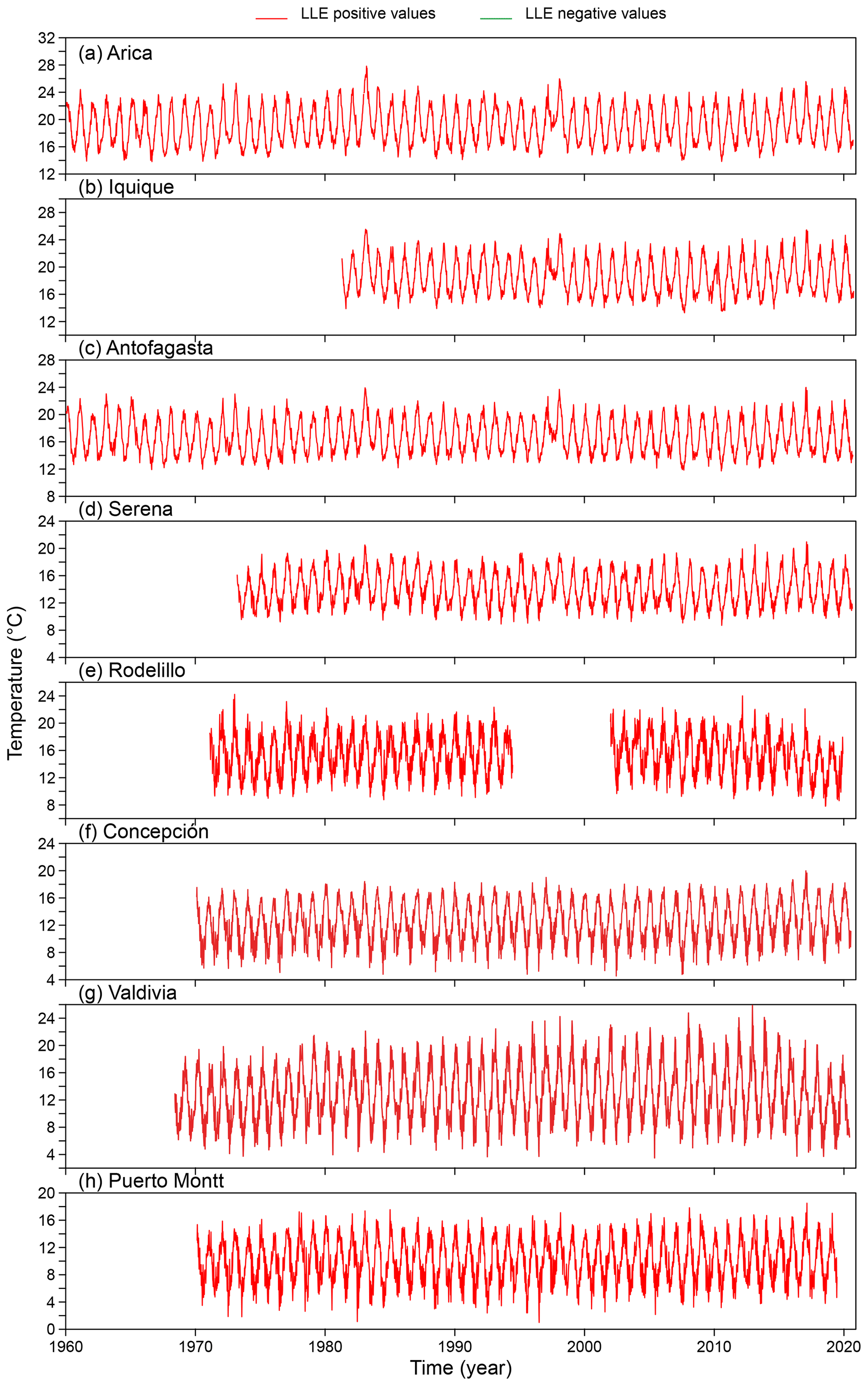
Figure D4Temperature record for atmospheric stations with superimposed information on 1-month local Lyapunov exponents: positive values for the LLEs are shown in red, and negative values are shown in green. Stations are given in a latitudinal arrangement.
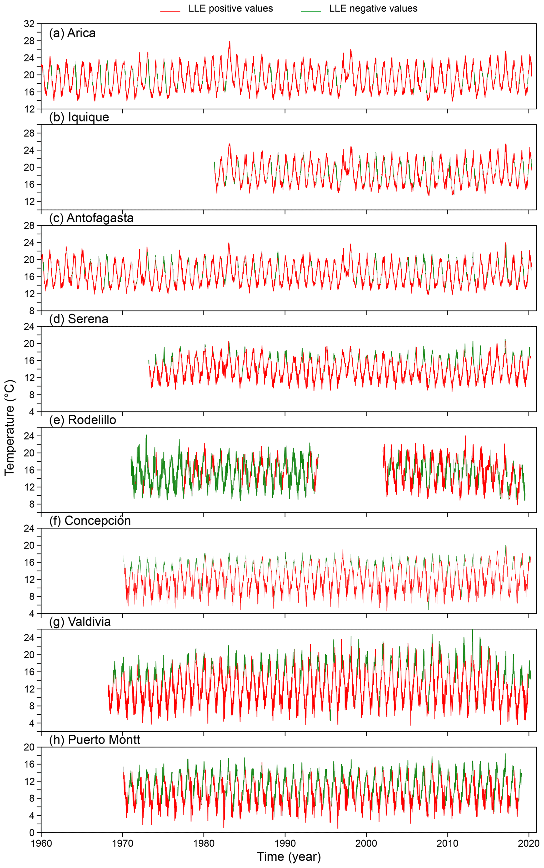
Figure D5Temperature record for atmospheric stations with superimposed information on 6-month local Lyapunov exponents: positive values for the LLEs are shown in red, and negative values are shown in green. Stations are given in a latitudinal arrangement.
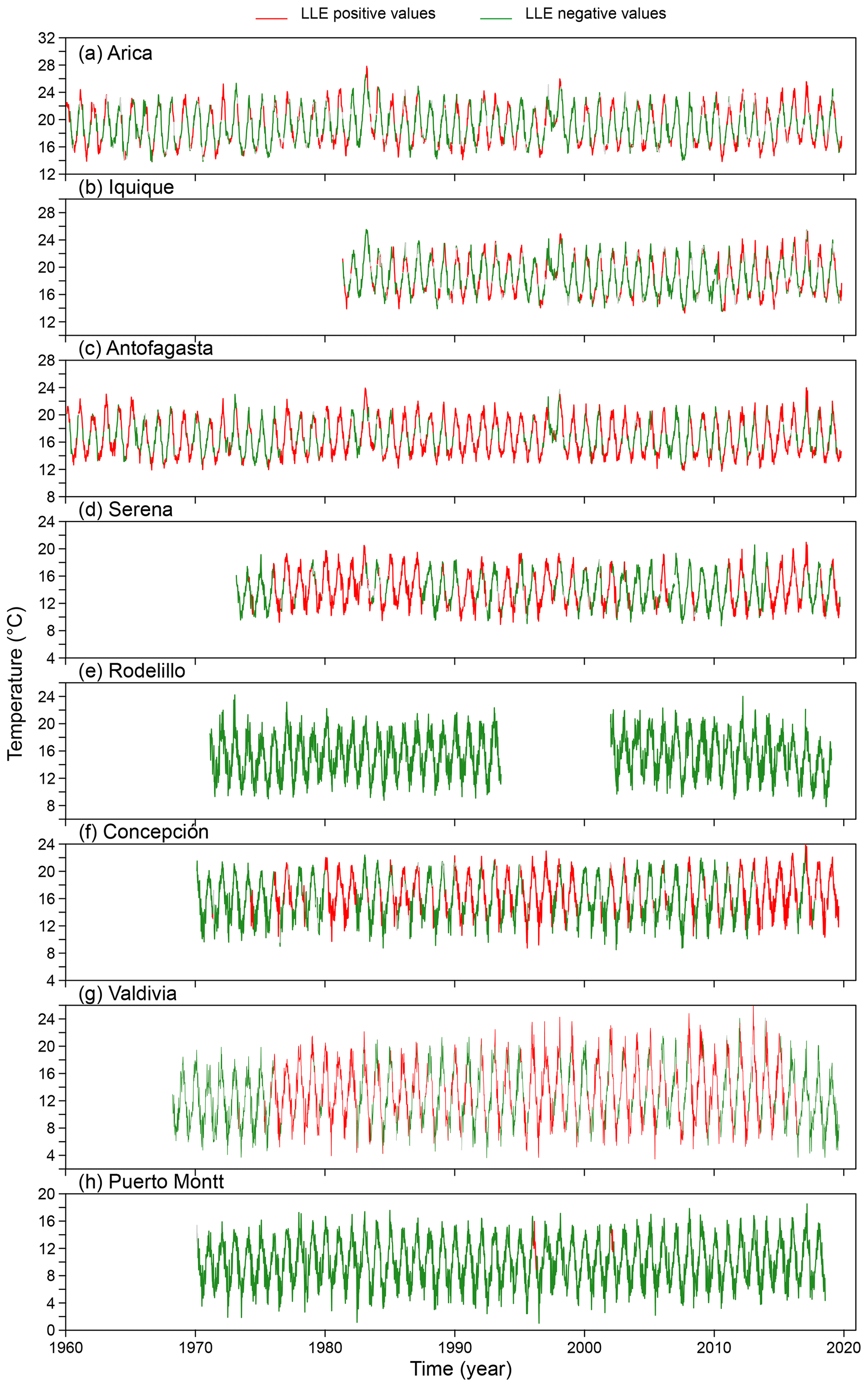
Figure D6Temperature record for atmospheric stations with superimposed information on 1-year local Lyapunov exponents: positive values for the LLEs are shown in red, and negative values are shown in green. Stations are given in a latitudinal arrangement.
Let {Xt} and {Yt} (t∈ℕ) be two stationary random processes, where , and . Then, the metric entropy Sρ at lag k is a normalized version of the Bhattacharya–Hellinger–Matusita distance, defined as
In the case where Yt=Xt for all t, Sk measures the serial dependence of {Xt} at lag k and can be interpreted as a nonlinear autocorrelation and cross-correlation function that overcomes the limits of Pearson's correlation coefficient. As pointed out in Maasoumi (1993), Granger et al. (2004) and Giannerini et al. (2015), Sρ satisfies many desirable properties, including the seven Rényi axioms and the additional properties described in Maasoumi (1993). We compute the cross-entropy tests for dependence as detailed in Giannerini and Goracci (2023). The estimator of Sk is based on univariate and bivariate nonparametric kernel density estimation and numerical integration. The confidence bands are derived under the null hypothesis of mutual independence between series. In Figures E1–E6 we show the results of the cross-entropy test between the ONI and LLEs for the oceanic stations with a time horizon of 1 and 6 months, as well as for the atmospheric stations with a time horizon of 1 month. For Serena we also tested the 1-year-ahead LLEs; see Fig. E7. For the atmospheric stations, only 1-month LLEs are shown, since no relationship was found between the ONI and 6-month-ahead LLEs.
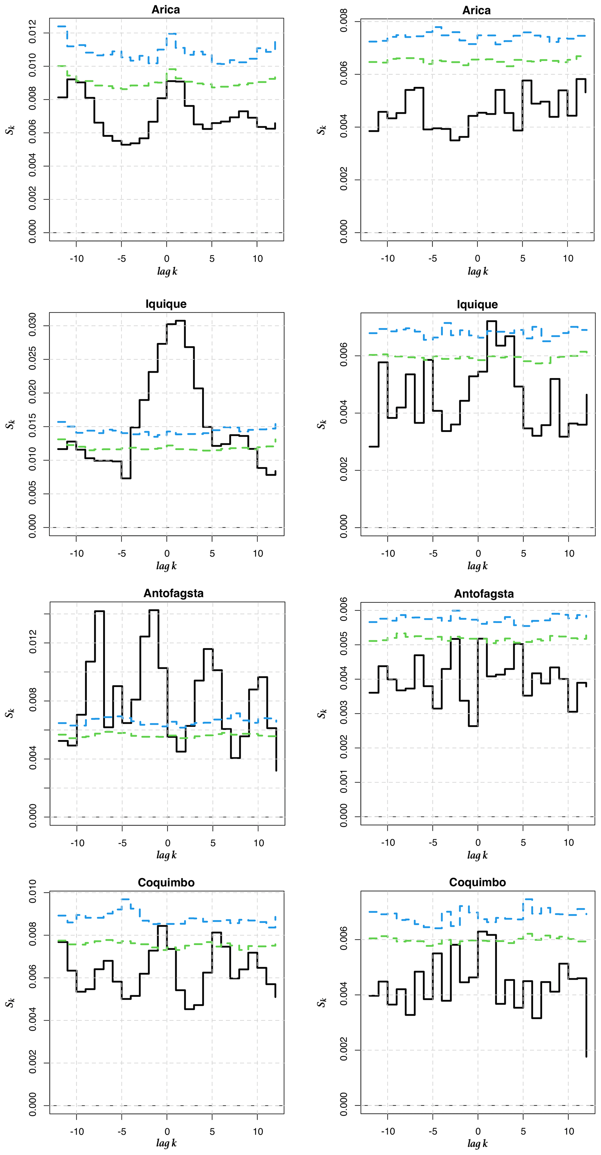
Figure E1Cross-entropy Sk for between the 1-month LLEs (SST) and the ONI for the first four stations. Left: original time series. Right: pre-whitened time series.
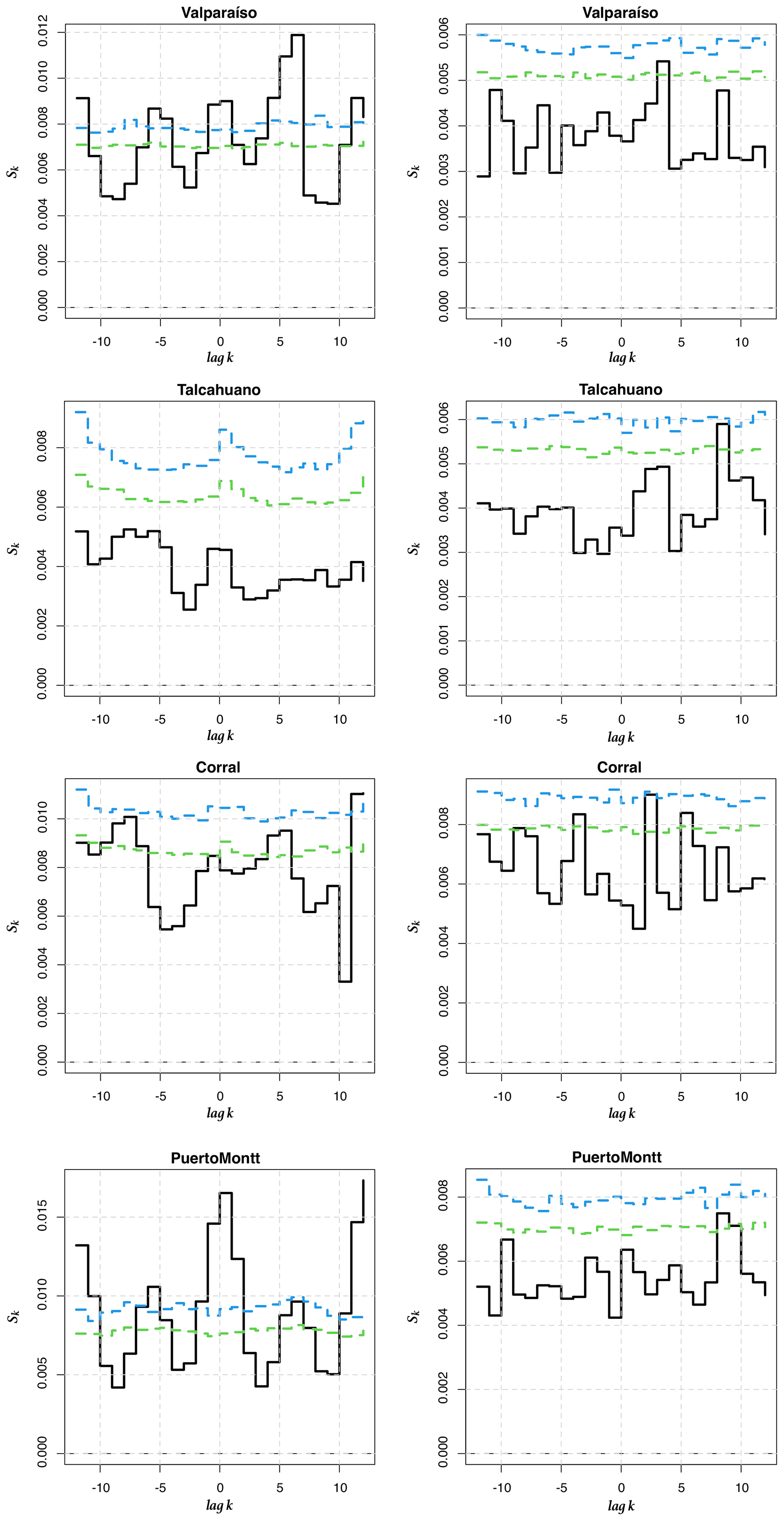
Figure E2Cross-entropy Sk for between the 1-month LLEs (SST) and the ONI or the last four stations. Left: original time series. Right: pre-whitened time series.
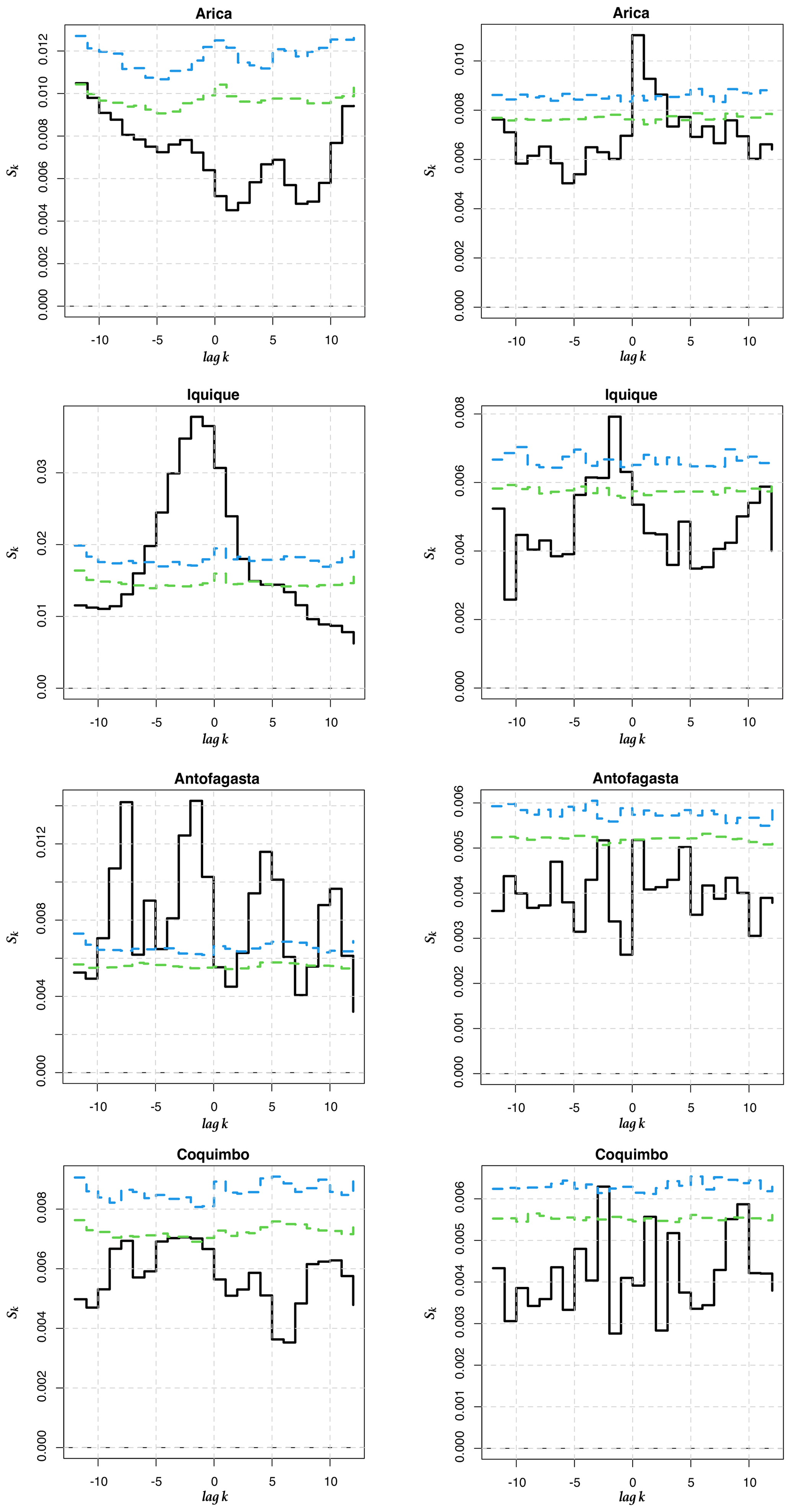
Figure E3Cross-entropy Sk for between the 6-month LLEs (SST) and the ONI for the first four stations. Left: original time series. Right: pre-whitened time series.
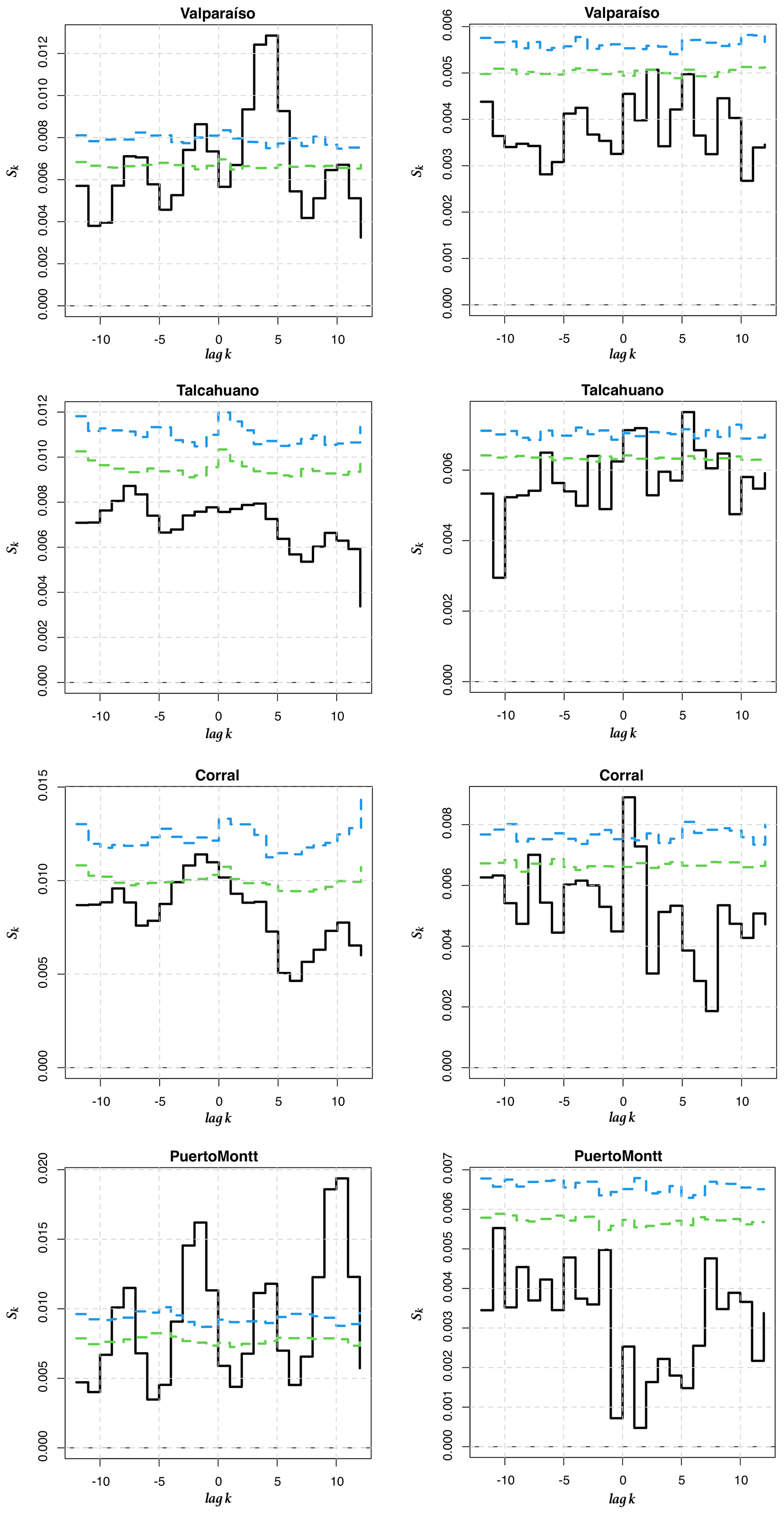
Figure E4Cross-entropy Sk for between the 6-month LLEs (SST) and the ONI for the last four stations. Left: original time series. Right: pre-whitened time series.
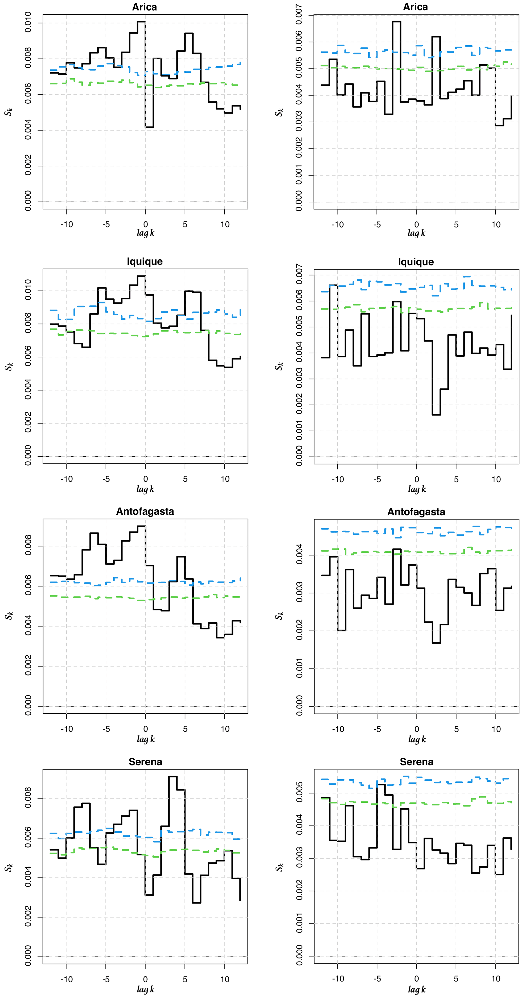
Figure E5Cross-entropy Sk for between the 1-month LLEs (AST) and the ONI for the first four stations. Left: original time series. Right: pre-whitened time series.
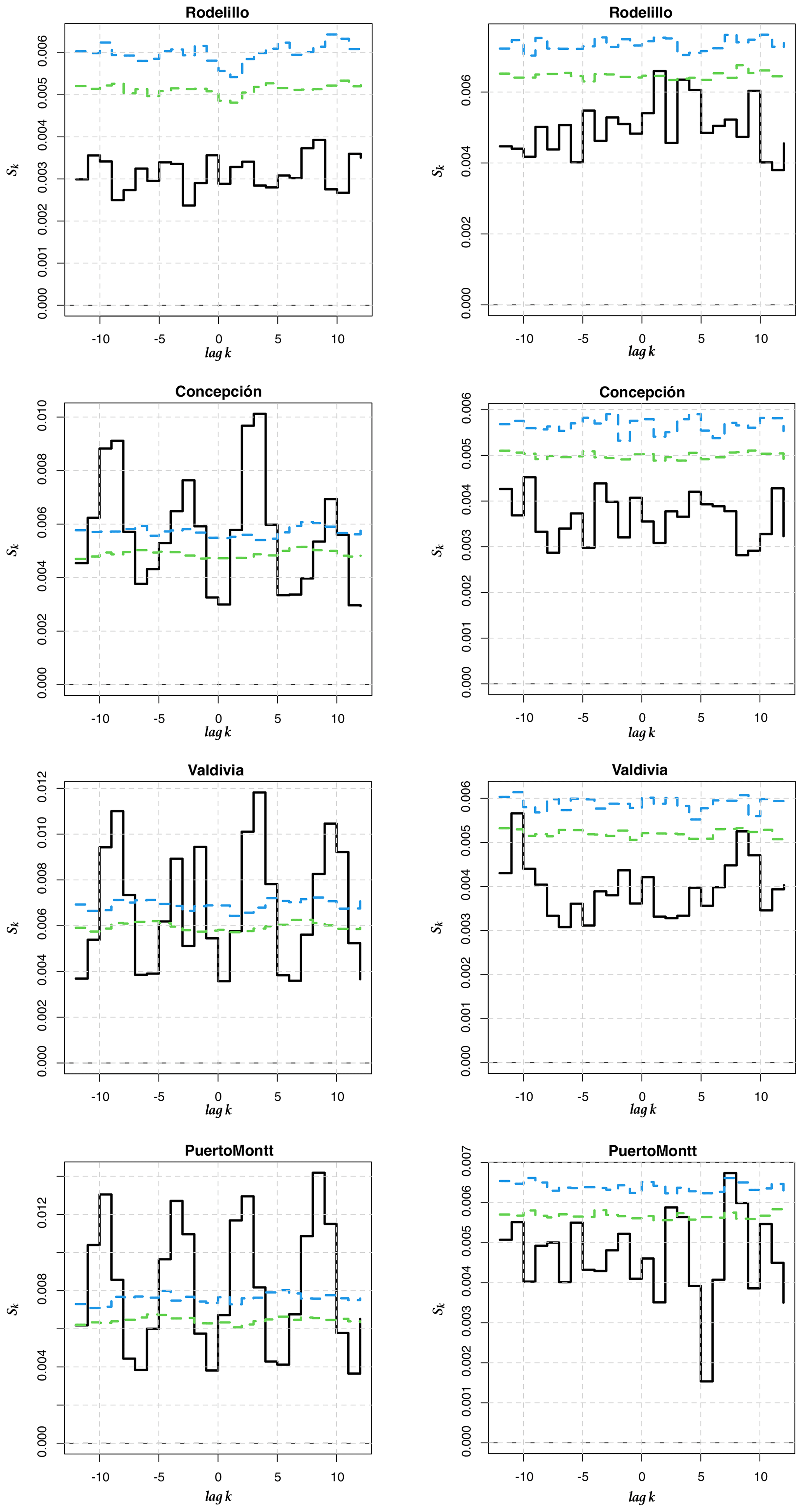
Figure E6Cross-entropy Sk for between the 1-month LLEs (AST) and the ONI for the last four stations. Left: original time series. Right: pre-whitened time series.
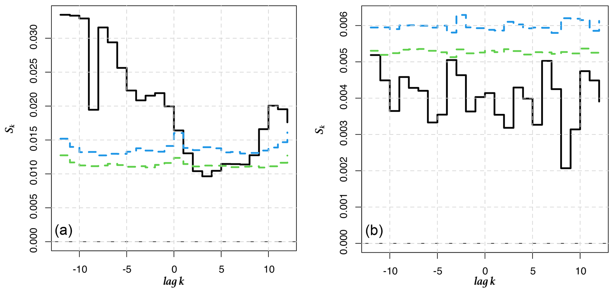
Figure E7Cross-entropy Sk for between the 1-year LLEs for La Serena and the ONI. (a) Original time series. (b) Pre-whitened time series.
We obtained access to Chilean naval temperature data; the rights to those data remain with the navy. Access to the data is by request to the Hydrographic and Oceanographic Service of the Chilean Navy (SHOA).
BRG, SG and JHEC participated in the development, design, calculations, elaboration of the figures and the results and produced a first draft of the article. DASdL, VVG and BRG participated in the discussion of the results. MC provided all the data and helped with the development of the first ideas. All authors read and approved the final paper.
The contact author has declared that none of the authors has any competing interests.
Publisher's note: Copernicus Publications remains neutral with regard to jurisdictional claims made in the text, published maps, institutional affiliations, or any other geographical representation in this paper. While Copernicus Publications makes every effort to include appropriate place names, the final responsibility lies with the authors.
Berenice Rojo-Garibaldi would like to thank Christof Jung and Thomas Seligman of the Institute of Physical Sciences, UNAM, Campus Cuernavaca, Mexico, for their helpful comments during the course of this work.
We acknowledge support of the publication fee by the CSIC Open Access Publication Support Initiative through its Unit of Information Resources for Research (URICI).
This paper was edited by Michel Crucifix and reviewed by Michel Crucifix and one anonymous referee.
Abarbanel, H., Brown, R., and Kennel, M.: Local Lyapunov exponents computed from observed data, J. Nonlinear Sci., 2, 343–365, 1992. a
Acosta-Jamett, G., Gutiérrez, J., Kelt, D., Meserve, P., and Previtali, M.: El Niño Southern Oscillation drives conflict between wild carnivores and livestock farmers in a semiarid area in Chile, J. Arid Environ., 126, 76–80, https://doi.org/10.1016/j.jaridenv.2015.08.021, 2016. a
Bailey, A., Ellner, S., and Nychka, W.: Chaos with confidence : Asymtotics and Applications of local Lyapounov exponents, Fields Institute Communications, 00, 1997. a
Barbieri, B., Bravo, M., Farías, M., González, A., Pizarro, O., and Yáñez, E.: Phenomena associated with the sea surface thermal structure observed through satellite images in the north of Chile, Invest. Mar. Valparaíso, 23, 99–122, https://doi.org/10.4067/S0717-71781995002300007, 1995. a, b
Bardgett, R., Freeman, C., and Ostle, N.: Microbial contributions to climate change through carbon cycle feedbacks, ISME J., 2, 805–814, https://doi.org/10.1038/ismej.2008.58, 2008. a
Bé, A. and Tolderlund, D.: Distribution and ecology of living planktonic foraminifera in surface waters of the Atlantic and Indian oceans, in: The micropaleontology of the oceans, edited by: Furnell, B. and Riedel, W., Cambridge University Press, ISBN: 9780521187480, 105–149, 1971. a
Black, D., Hameed, S., and Peterson, L.: Long-term tidal cycle influences on a Late–Holocene clay mineralogy record from the Cariaco Basin, Earth Planet. Sc. Lett., 279, 139–146, https://doi.org/10.1016/j.epsl.2008.12.040, 2009. a
Bradford, A., McCulley, L., Crowther, W., Oldfield, E., Wood, A., and Fierer, N.: Cross-biome patterns in soil microbial respiration predictable from evolutionary theory on thermal adaptation, Nature Ecology and Evolution, 3, 223–231, https://doi.org/10.1038/s41559-018-0771-4, 2019. a
Bradley, E. and Kantz, H.: Nonlinear time-series analysis revisited, Chaos, 25, 097610-1-10, https://doi.org/10.1063/1.4917289, 2015. a
Camus, P.: Marine biogeography of continental Chile, Rev. Chil. Hist. Nat., 74, 587–617, 2001. a, b
Castro, R., González, V., Claramunt, G., Barrientos, P., and Soto, S.: Stable isotopes (Delta3C, Delta15N) seasonal changes in particulate organic matter and in different life stages of anchoveta (Engraulis ringens) in response to local and large scale oceanographic variations in north and central Chile, Prog. Oceanogr., 186, 1–2, https://doi.org/10.1016/j.pocean.2020.102342, 2020. a
Chan, K. and Tong, H.: Chaos: a statistical perspective, Springer-Verlag, https://doi.org/10.1007/978-1-4757-3464-5, 2001. a, b
Cuculeanu, V. and Lupu, A.: Deterministic chaos in Atmospheric radon dynamics, J. Geophys. Res.-Atmos., 106, 17961–17968, https://doi.org/10.1029/2001JD900148, 2001. a
Daneri, G., Dellarossa, V., Quiñones, R., Jacob, B., Montero, P., and Ulloa, O.: Primary production and community respiration in the Humboldt Current System off Chile and associated oceanic areas, Mar. Ecol. Prog. Ser., 197, 41–49, https://doi.org/10.3354/meps197041, 2000. a
Devlin, A., Jay, D., Talke, S., Zaron, E., Pan, J., and Lin, H.: Coupling of sea level and tidal range changes, with implications for future water levels, Sci. Rep.-UK, 7, https://doi.org/10.1038/s41598-017-17056-z, 2017a. a
Devlin, A., Jay, D., Zaron, E., Talke, S., Pan, J., and Lin, H.: Tidal variability related to sea level variability in the Pacific Ocean, J. Geophys. Res.-Oceans, 122, 8445–8463, https://doi.org/10.1002/2017JC013165, 2017b. a
Devlin, A., Pan, J., and Lin, H.: Extended spectral analysis of tidal variability in the North Atlantic Ocean, J. Geophys. Res.-Oceans, 124, 506–526, https://doi.org/10.1029/2018JC014694, 2019. a
Ellner, S., Nychka, D., and Gallant, A.: LENNS, a program to estimate the dominant Lyapunov exponent of noisy nonlinear systems from time series data, Institute of Statistics Mimeo Series, BMA Series 39, 2235, 1992. a
Elsner, J. and Tsonis, A.: Nonlinear prediction, chaos, and noise, B. Am. Meteorol. Soc., 73, 49–60, https://doi.org/10.1175/1520-0477(1992)073<0049:NPCAN>2.0.CO;2, 1992. a
Enfield, D. and Allen, J.: On the structure and dynamics of monthly mean sea level anomalies along the Pacific coast of north and south America, J. Phys. Oceanogr., 10, 557–578, https://doi.org/10.1175/1520-0485(1980)010<0557:OTSADO>2.0.CO;2, 1980. a, b
Fagel, N., Boës, X., and Loutre, M.: Climate oscillations evidenced by spectral analysis of Southern Chilean lacustrine sediments: the assessment of ENSO over the last 600 years, J. Paleolimnol., 39, 253–266, 2008. a
Falvey, M. and Garreaud, R.: Regional cooling in a warming world: recent temperature trends in the southeast Pacific and along the west coast of subtropical South America (1979–2006), J. Geophys. Res.-Atmos., 114, 1–16, https://doi.org/10.1029/2008JD010519, 2009. a
Fan, J., Meng, J., Ashkenazy, Y., Havlin, S., and Schellnhuber, J.: Network analysis reveals strongly localized impacts of El Niño, P. Natl. Acad. Sci. USA, 114, 7543–7548, https://doi.org/10.1073/pnas.1701214114, 2017. a
Fedorov, A.: The response of the coupled tropical ocean-atmosphere to westerly wind bursts, Q. J. Roy. Meteor. Soc., 128, 1–23, 2002. a
Fedorov, A., Harper, S., Philander, S., Winter, B., and Wittenberg, A.: How predictable is El Niño?, B. Am. Meteorol. Soc., 84, 911–920, https://doi.org/10.1175/BAMS-84-7-911, 2003. a
Fogt, R. and Bromwich, D.: Decadal variability of the ENSO teleconnection to the high-latitude South Pacific governed by coupling with the southern annular mode, J. Climate, 19, 979–997, https://doi.org/10.1175/JCLI3671.1, 2006. a
Friedrich, M., Smeekes, S., and Urbain, J.: Autoregressive wild bootstrap inference for nonparametric trends, J. Econometrics, 214, 81–109, https://doi.org/10.1016/j.jeconom.2019.05.006, 2020. a, b
Fuenzalida, R.: Aspectos oceanográficos y meteorológicos de El Niño 1982–83 en la zona costera de Iquique, Invest. Pesq., 32, 47–52, 1985. a
Garreaud, R.: Record–breaking climate anomalies lead to severe drought and environmental disruption in western Patagonia in 2016, Clim. Res., 74, 217–229, https://doi.org/10.3354/cr01505, 2018. a
Garreaud, R., Lopez, P., Minvielle, M., and Rojas, M.: Large-scale control on the Patagonian climate, J. Climate, 26, 215–230, https://doi.org/10.1175/JCLI-D-12-00001.1, 2013. a
Giannerini, S. and Goracci, G.: Entropy-Based Tests for Complex Dependence in Economic and Financial Time Series with the R Package tseriesEntropy, Mathematics, 11, 2–27, https://doi.org/10.3390/math11030757, 2023. a, b
Giannerini, S. and Rosa, R.: New resampling method to assess the accuracy of the maximal Lyapunov exponent estimation, Physica D, 155, 101–111, 2001. a, b
Giannerini, S. and Rosa, R.: Assessing chaos in time series: Statistical aspects and perspectives, Stud. Nonlinear Dyn. E., 8, 2004. a
Giannerini, S., Maasoumi, E., and Dagum, E.: Entropy Testing for Nonlinear Serial Dependence in Time Series, Biometrika, 102, 661–675, https://doi.org/10.1093/biomet/asv007, 2015. a, b
Gillett, N., Kell, T., and Jones, P.: Regional climate impacts of the Southern Annular Mode, Geophys. Res. Lett., 33, L23704, https://doi.org/10.1029/2006GL027721, 2006. a
Glantz, M.: Introduction to El Niño, Springer Nature, https://doi.org/10.1007/978-3-030-86503-0, p. 375, 2022. a
Gómez, R.: Variabilidad Ambiental y pequeños pelágicos de la zona norte y centro–sur de Chile, Master's thesis, Universidad de Concepción, 2008. a
González-Reyes, Á and. Muñoz, A.: Precipitation changes of Valdivia city (Chile) during the past 150 years, Bosque (Valdivia), 34, 200–213, https://doi.org/10.4067/S0717-92002013000200008, 2013. a
Granger, C., Maasoumi, E., and Racine, J.: A Dependence Metric for Possibly Nonlinear Processes, J. Time Ser. Anal., 25, 649–669, 2004. a
Grassberger, P.: Is there a climatic attractor?, Nature, 323, 609–612, https://doi.org/10.1038/323609a0, 1986. a
Gratiot, N., Anthony, E., Gardel, A., Gaucherel, C., Proisy, C., and Wells, J.: Significant contribution of the 18.6 year tidal cycle to regional coastal changes, Nat. Geosci., 1, 169–172, https://doi.org/10.1038/ngeo127, 2008. a
Guera, C. and Portflitt, G.: El Niño effects on pinnipeds in northern Chile, Pinnipeds and El Niño: Responses to Environmental Stress, edited by: Trillmich, F. and Ono, K. A., Springer Berlin Heidelberg, vol. 88, pp. 47–54, https://doi.org/10.1007/978-3-642-76398-4_5, 1991. a
Gutiérrez, J. and Meserve, P.: El Niño effects on soil seed bank dynamics in north–central Chile, Oecologia, 134, 511–517, https://doi.org/10.1007/s00442-002-1156-5, 2003. a
Harris, R., Beaumont, L., Vance, T., Tozer, C., Remenyi, T., Perkins-Kirkpatrick, S., Mitchell, P. J., Nicotra, A., McGregor, S., Andrew, N., Letnic, M., Kearney, M., Wernberg, T., Hutley, L., Chambers, L., Fletcher, M., Keatley, M., Woodward, C., Williamson, G., Duke, N., and Bowman, D.: Biological responses to the press and pulse of climate trends and extreme events, Nat. Clim. Change, 8, 579–587, https://doi.org/10.1038/s41558-018-0187-9, 2018. a, b
Holmgren, M., Scheffer, M., Ezcurra, E., Gutiérrez, J., and Mohren, G.: El Niño effects on the dynamics of terrestrial ecosystems, Trends Ecol. Evol., 16, 89–94, https://doi.org/10.1016/S0169-5347(00)02052-8, 2001. a
Hormazabal, S., Shaffer, G., Letelier, J., and Ulloa, O.: Local and remote forcing of sea surface temperature in the coastal upwelling system off Chile, J. Geophys. Res.-Oceans, 106, 16657–16671, https://doi.org/10.1029/2001JC900008, 2001. a
Houghton, J., Ding, Y., Griggs, D., Noguer, M., van der Linden, P., Dai, X., Maskell, K., and Johnson, C., eds.: IPCC, 2001: Climate Change 2001: The Scientific Basis: Contribution of Working Group I to the Third Assessment Report of the Intergovernmental Panel on Climate Change, https://doi.org/10.1002/joc.763, 2001. a
Ihlow, F., Courant, J., Secondi, J., Herrel, A., Rebelo, R., Measey, G., Lillo, F., De Villers, F., Vogt, S., De Busschere, C., Backeljau, T., and Rodder, D.: Impacts of Climate Change on the Global Invasion Potential of the African Clawed Frog Xenopus laevis, PLOS ONE, 11, https://doi.org/10.1371/journal.pone.0154869, 2015. a
Jiang, F., Zhang, W., Stuecker, M., and Jin, F.: Decadal change of combination mode spatiotemporal characteristics due to an ENSO regime shift, J. Climate, 33, 5239–5251, 2020. a
Joos, F.: Growing feedback from ocean carbon to climate, Nature, 522, 295–296, https://doi.org/10.1038/522295a, 2015. a
Kalnay, E.: Atmospheric Modeling, Data Assimilation, and Predictability, Cambridge University Press, ISBN: 9780521796293, 2003. a
Kalthoff, N., BischoffeGauß, I., FiebigeWittmaack, M., Fiedler, F., Thuerauf, J., Novoa, E., Pizarro, C., Castillo, R., Gallardo, L., Rondanelli, R., and Kohler, M.: Mesoscale wind regimes in Chile at 30∘ S, J. Appl. Meteorol, 41, 953–970, https://doi.org/10.1175/1520-0450(2002)041<0953:MWRICA>2.0.CO;2, 2002. a
Kantz, H.: A robust method to estimate the maximal Lyapunov exponent of a time series, Phys. Lett. A, 185, 77–87, 1994. a
Kovats, R., Bouma, M., Hajat, S., Worrall, E., and Haines, A.: El Niño and health, Lancet, 362, 1481–9, https://doi.org/10.1016/S0140-6736(03)14695-8, 2003. a
Lorenz, E.: Deterministic Nonperiodic Flow, J. Atmos. Sci, 20, 130–141, https://doi.org/10.1175/1520-0469(1963)020<0130:DNF>2.0.CO;2, 1963. a, b
Lorenz, E.: Dimension of weather and climate attractors, Nature, 353, 241–244, https://doi.org/10.1038/353241a0, 1991. a
Lubchenco, J., Navarrete, S., Tissol, B., and Castilla, J.: Possible ecological responses to global climate change Nearshore benthic biota of northeastern Pacific coastal ecosystems, Contrasts between North and South America, in: Earth System Responses to Global Change: Contrasts between North and South America, edited by: Mooney, H. A., Fuentes, E. R., and Kronberg, B. I., ISBN: 9780125053006, 147–166, 1993. a
Maasoumi, E.: A Compendium to Information Theory in Economics and Econometrics, Economet. Rev., 12, 137–181, 1993. a, b
Mayol, E., Ruiz-Halpern, S., Duarte, C. M., Castilla, J. C., and Pelegrí, J. L.: Coupled CO2 and O2-driven compromises to marine life in summer along the Chilean sector of the Humboldt Current System, Biogeosciences, 9, 1183–1194, https://doi.org/10.5194/bg-9-1183-2012, 2012. a, b
Montecino, V., Strub, T., Chavez, F., Thomas, A., Tarazona, J., and Baumgartner, T.: Bio-physical interactions off Western South-America, in: The sea. The Global Coastal Ocean: Interdisciplinary Regional Studies and Synthesis, edited by: Robinson, A. and Brink, K., vol. 14A, pp. 1–49, Harvard Press, ISBN 9780674015272, 2006. a
Montecinos, A. and Gomez, F.: ENSO modulation of the upwelling season off southern-central Chile, Geophys. Res. Lett., 37, L02708, https://doi.org/10.1029/2009GL041739, 2010. a
Montecinos, S., Gutierrez, J., Lopez-Cortes, F., and Lopez, D.: Climatic characteristics of the semi-arid Coquimbo Region in Chile, Journal of Arid Enviroments, 126, 7–11, https://doi.org/10.1016/j.jaridenv.2015.09.018, 2015. a
Montero, P., Daneri, G., Cuevas, L., González, H., Jacob, B., Lizárraga, L., and Menschel, E.: Productivity cycles in the coastal upwelling area off Concepción: the importance of diatoms and bacterioplankton in the organic carbon flux, Prog. Oceanogr., 75, 518–530, https://doi.org/10.1016/j.pocean.2007.08.013, 2007. a
Moritz, S. and Bartz-Beielstein, T.: imputeTS: Time Series Missing Value Imputation in R, R J., 9, 207–218, https://doi.org/10.32614/RJ-2017-009, 2017. a
Namias, J.: Multiple causes of the North American abnormal winter 1976–1977, Mon. Weather Rev., 106, 279–295, 1978. a
Nicolis, C. and Nicolis, G.: Do climatic attractor exist?, Nature, 331, 529–532, https://doi.org/10.1038/311529a0, 1984. a
Núñez, J., Rivera, D., Oyarzún, R., and Arumí, J.: Influence of Pacific Ocean multidecadal variability on the distributional properties of hydrological variables in north-central Chile, J. Hydrol., 501, 227–240, https://doi.org/10.1016/j.jhydrol.2013.07.035, 2013. a
Nychka, D., Ellner, S., McCaffrey, D., and Gallant, A.: Finding Chaos in Noisy Systems, J. Roy. Stat. Soc. B-Meth., 54, 399–426, 1992. a
Oost, A., De Haas, H., Ijnsen, F., Van den Boogert, J., and De Boer, P.: The 18.6 yr nodal cycle and its impact on tidal sedimentation, Sediment. Geol., 87, 1–11, https://doi.org/10.1016/0037-0738(93)90032-Z, 1993. a
Pauly, D. and Christensen, V.: Primary production required to sustain global fisheries, Nature, 374, 255–257, https://doi.org/10.1038/374255a0, 1995. a
Petkov, B., Vitale, V., Mazzola, M., Lanconelli, C., and Lupi, A.: Chaotic behaviour of the short-term variations in ozone column observed in Arctic, J. Geophys. Res.-Atmos., 26, 238–249, https://doi.org/10.1016/j.cnsns.2015.02.020, 2015. a
Pierrehumbert, R.: Dimensions of Atmospheric variability, in: Beyond Belief: randomness, Prediction and Explanation in Science, edited by: Casti, J. L. and Karlqvist, A., pp. 110–142, CRC Press, ISBN: 9780849342912, 1990. a
Piñones, A., Castilla, J., Guiñez, R., and Largier, J.: Nearshore surface temperatures in Antofagasta Bay (Chile) and adjacent upwelling centers, Cienc. Mar., 33, 37–48, https://doi.org/10.7773/cm.v33i1.1226, 2007. a, b
Pizarro, A., Hormazabal, F., González, C., and Yanez, R.: Variabilidad del viento, nivel del mar y temperatura en la costa norte de Chile, Investigaciones Marinas, 22, 85–101, https://doi.org/10.4067/S0717-71781994002200007, 1994. a
Pizarro, O. and Montecinos, A.: El Niño y la Oscilación Sur, in: Biología Marina y Oceanografía: Conceptos y Procesos, edited by: Werlinger, C., Alveal, K., and Romo, H., vol. 1, pp. 197–224, Universidad de Concepción, ISBN: 9789568436001, 2004. a, b
Riveros, Z., Yustres, Q., and Ivanova, Y.: Efecto del fenómeno de la Oscilación Cuasi–Bienal en los afluentes del embalse de Betania, Revista EIA, 17, 1–9, https://doi.org/10.24050/reia.v17i34.1246, 2020. a
Rosenstein, M., Collins, J., and De Luca, C.: A practical method for calculating largest Lyapunov exponents from small data sets, Physica D, 65, 117–134, 1993. a
Rossiter, J.: Long term variations in sea level, in: The Sea, edited by: Hill, M. N., Interscience, New York, Vol. 1, ISBN: 9780471044024, 1962. a
Rutllant, J. and Fuenzalida, H.: Synoptic aspects of central rainfall variability associated with the Southern Oscillation, Int. J. Climatol., 11, 63–76, https://doi.org/10.1002/joc.3370110105, 1991. a
Sakova, I., Meyers, G., and Coleman, R.: Interannual variability in the Indian Ocean using altimeter and IX1-expendable bathy-thermograph (XBT) data: Does the 18-month signal exist?, Geophys. Res. Lett., 33, L20603, https://doi.org/10.1029/2006GL027117, 2006. a
Sarricolea, P., Herrera-Ossandon, M., and Meseguer-Ruiz, Ó.: Climatic regionalisation of continental Chile, J. Maps, 13, 66–73, https://doi.org/10.1080/17445647.2016.1259592, 2017. a
Shaffer, G., Pizarro, O., Djurfeldt, L., Salinas, S., and Rutland, J.: Circulation and low frequency variability near the Chilean coast: remotely forced fluctuations during the 1991–1992 El Niño, J. Phys. Oceanogr., 27, 217–235, https://doi.org/10.1175/1520-0485(1997)027<0217:CALFVN>2.0.CO;2, 1997. a, b
Shaffer, G., Hormazábal, S., Pizarro, O., and Salinas, S.: Seasonal and interannual variability of current and temperature off center Chile, J. Geophys. Res., 104, 29951–29961, https://doi.org/10.1029/1999JC900253, 1999. a
Shintani, M. and Linton, O.: Nonparametric neural network estimation of Lyapunov exponents and a direct test for chaos, J. Econometrics, 120, 1–33, 2004. a, b, c
Sievers, A. and Silva, N.: Water masses and circulation in austral Chilean channels and fjords, in: Progress in the Oceanographic Knowledge of Chilean Inner Waters, from Puerto Montt to Cape Horn, edited by: Silva, N. and Palma, S., Comité Oceanográfico Nacional – Pontificia Universidad Católica de Valparaíso, Valparaíso, 53–58, 2008. a
Smith, A., Guastella, L., Bundy, S., and Mather, A.: Combined marine storm and Saros spring high tide erosion events along the KwaZulu–Natal coast in March 2007: News and views, S. Afr. J. Sci., 103, 274–276, 2007. a
Smith, L. A.: Identification and prediction of low dimensional dynamics, Physica D, 58, 50–76, 1992. a
Sobarzo, M., Bravo, L., Donoso, D., Garces-Vargas, J., and Schneider, W.: Coastal upwelling and seasonal cycles that influence the water column over the continental shelf off central Chile, J. Prog. Oceanogr., 75, 363–382, https://doi.org/10.1016/j.pocean.2007.08.022, 2007. a
Solomon, S., Qin, D., Manning, M., Chen, Z., Marquis, M., Averyt, K., Tignor, M., and Miller, H., eds.: Climate Change 2007: The Physical Science Basis. Contribution of Working Group I to the Fourth Assessment Report of the Intergovernmental Panel on Climate Change, IPCC, Cambridge University Press, 2007a. a
Soto, M., Julio-Alvear, G., and Salinas, R.: Current Wildfire Risk Status and Forecast in Chile: Progress and Future Challenges, in: Wildfire Hazards, Risks, and Disasters, edited by: Shroder, J. and Paton, D., chap. 4, Elsevier, https://doi.org/10.1016/B978-0-12-410434-1.00004-X, 2015. a
Stramma, L., Johnson, G., Sprintall, J., and Mohrholz, V.: Expanding oxygen-minimum zones in the tropical oceans, Science, 320, 655–658, https://doi.org/10.1126/science.1153847, 2008. a
Stuecker, M., Timmermann, A., Jin, F., McGregor, S., and Ren, H.: A combination mode of the annual cycle and the El Niño/Southern Oscillation, Nat. Geosci., 6, 540–544, 2013. a
Stuecker, M., Timmermann, A., Jin, F., Chikamoto, Y., Zhang, W., Wittenberg, A., Widiasih, E., and Zhao, S.: Revisiting ENSO/Indian Ocean dipole phase relationships, Geophys. Res. Lett., 44, 2481–2492, 2017. a
Sydeman, W., Garcia-Reyes, M., Schoeman, D., Rykaczewski, R., Thompson, S., Black, B., and Bograd, S.: Climate change and wind intensification in coastal upwelling ecosystems, Science, 345, 77–80, https://doi.org/10.1126/science.1251635, 2014. a
Thompson, P.: Uncertainty of initial state as a factor in the predictability of large scale atmospheric patterns, Tellus, 9, 275–295, https://doi.org/10.3402/tellusa.v9i3.9111, 1963. a
Thompson, P., Widlansky, M., Hamlington, B., Merrifield, M., Marra, J., Mitchum, G., and Sweet, W.: Rapid increases and extreme months in projections of United States high-tide flooding, Nat. Clim. Change, 11, 584–590, https://doi.org/10.1038/s41558-021-01077-8, 2021. a
Tong, H.: A personal overview of nonlinear time series analysis from a chaos perspective, Scand. J. Stat., 22, 399–445, 1995. a
Tsonis, A., Elsner, J., and Georgakakos, K.: Estimating the Dimension of the Weather and Climate Attractors: Important Issues about the Procedure and Interpretation, J. Atmos. Sci., 50, 2549–2555, https://doi.org/10.1175/1520-0469(1993)050<2549:ETDOWA>2.0.CO;2, 1993. a
Ulloa, O., Escribano, R., Hormazabal, S., Quiñones, R., and González, R.: Evolution and biological effects of the 1997–1998 El Niño in the upwelling ecosystem off northern Chile, Geophys. Res. Lett., 28, 1591–1594, https://doi.org/10.1029/2000GL011548, 2001. a
Urrutia-Jalabert, R., González, M., González-Reyes, A., Lara, A., and Garreaud, R.: Climate variability and forest fires in central and south-central Chile, Ecosphere, 9, e02171, https://doi.org/10.1002/ecs2.2171, 2018. a, b
Vannitsem, S., Demaeyer, J., De Cruz, L., and Ghil, M.: Low-frequency variability and heat transport in a low-order nonlinear coupled ocean-atmosphere model, Physica D, 309, 71–85, 2015. a
Vargas, G., Pantoja, S., Rutllant, J., Lange, C., and Ortlieb, L.: Enhancement of coastal upwelling and interdecadal ENSO-like variability in the Peru–Chile Current since late 19th century, Geophys. Res. Lett., 34, L13607, https://doi.org/10.1029/2006GL028812, 2007. a, b, c
Vassiliadis, D., Sharma, A., Eastman, T., and Papadopoulos, K.: Lyapunov exponent of magnetospheric activity from all time series, Geophys. Res. Lett., 18, 1841–1844, https://doi.org/10.1029/91GL01378, 1991. a
Venables, W. and Ripley, B.: Modern Applied Statistics with S, fourth edn., Springer, New York, https://www.stats.ox.ac.uk/pub/MASS4/ (last access: 30 October 2023), iSBN 0-387-95457-0, 2002. a
Vilina, Y., Cofré, H., Silva-García, C., García, M., and Pérez-Friedenthal, C.: Effects of El Niño on Abundance and Breeding of Black–Necked Swans on El Yali Wetland in Chile, Waterbird Society, 25, 123–127, 2002. a
Villalba, R., Cook, E., Jacoby, G., D'Arrigo, R., Veblen, T., and Jones, P.: Tree-ring based reconstructions of northern Patagonia precipitation since AD 1600, Holocene, 8, 659–674, 1998. a
Wang, S., Huang, J., He, Y., and Guan, Y.: Combined effects of the Pacific Decadal Oscillation and El Niño-Southern Oscillation on Global and Dry-Wet Changes, Sci .Rep.-UK, 4, 6651, https://doi.org/10.1038/srep06651, 2014. a
Wolff, R.: Local Lyapunov exponents: looking closely at chaos, J. R. Stat. Soc. B., 54, 353–371, 1992. a
Yao, Q. and Tong, H.: A personal overview of nonlinear time series analysis from a chaos perspective, J. R. Stat. Soc. B., 56, 701–725, 1994. a, b
Yeo, S. and Kim, K.: Decadal changes in the Southern Hemisphere sea surface temperature in association with El Niño-Southern Oscillation and Southern Annular Mode, Clim. Dynam., 45, 3227–3242, https://doi.org/10.1007/s00382-015-2535-z, 1992. a
Zeng, X., Pielke, A., and Eykholt, R.: Estimating the Fractal Dimension and the Predictability of the Atmosphere, J. Atmos. Sci., 49, 649–659, https://doi.org/10.1175/1520-0469(1992)049<0649:ETFDAT>2.0.CO;2, 2015. a
Ziehmann, C., Smith, L., and Kurths, J.: Localized Lyapunov exponents and the prediction of predictability, Phys. Lett. A, 271, 237–251, https://doi.org/10.1016/S0375-9601(00)00336-4, 2000. a
- Abstract
- Introduction
- Data and methods
- Results
- Discussion
- Conclusions
- Appendix A: The Humboldt Current System, El Niño–Southern Oscillation and Southern Annual Mode
- Appendix B: Spectral analysis
- Appendix C: Neural network models for random dynamical systems
- Appendix D: Local Lyapunov exponents
- Appendix E: Cross-entropy tests with the measure Sk
- Data availability
- Author contributions
- Competing interests
- Disclaimer
- Acknowledgements
- Financial support
- Review statement
- References