the Creative Commons Attribution 4.0 License.
the Creative Commons Attribution 4.0 License.
 | 10 Mar 2022
Quantifying memory and persistence in the atmosphere–land and ocean carbon system
Rostyslav Bun
Iryna Ryzha
Piotr Żebrowski
Here we intend to further the understanding of the planetary burden (and its dynamics) caused by the effect of the continued increase in carbon dioxide (CO2) emissions from fossil fuel burning and land use as well as by global warming from a new rheological (stress–strain) perspective. That is, we perceive the emission of anthropogenic CO2 into the atmosphere as a stressor and survey the condition of Earth in stress–strain units (stress in units of Pa, strain in units of 1) – allowing access to and insight into previously unknown characteristics reflecting Earth's rheological status. We use the idea of a Maxwell body consisting of elastic and damping (viscous) elements to reflect the overall behavior of the atmosphere–land and ocean system in response to the continued increase in CO2 emissions between 1850 and 2015. Thus, from the standpoint of a global observer, we see that the CO2 concentration in the atmosphere is increasing (rather quickly). Concomitantly, the atmosphere is warming and expanding, while some of the carbon is being locked away (rather slowly) in land and oceans, likewise under the influence of global warming.
It is not known how reversible and how out of sync the latter process (uptake of carbon by sinks) is in relation to the former (expansion of the atmosphere). All we know is that the slower process remembers the influence of the faster one, which runs ahead. Important questions arise as to whether this global-scale memory – Earth's memory – can be identified and quantified, how it behaves dynamically, and, last but not least, how it interlinks with persistence by which we understand Earth's path dependency.
We go beyond textbook knowledge by introducing three parameters that characterize the system: delay time, memory, and persistence. The three parameters depend, ceteris paribus, solely on the system's characteristic viscoelastic behavior and allow deeper and novel insights into that system. The parameters come with their own limits which govern the behavior of the atmosphere–land and ocean carbon system, independently from any external target values (such as temperature targets justified by means of global change research). We find that since 1850, the atmosphere–land and ocean system has been trapped progressively in terms of persistence (i.e., it will become progressively more difficult to relax the system), while its ability to build up memory has been reduced. The ability of a system to build up memory effectively can be understood as its ability to respond still within its natural regime or, if the build-up of memory is limited, as a measure for system failures globally in the future. Approximately 60 % of Earth's memory had already been exploited by humankind prior to 1959. Based on these stress–strain insights we expect that the atmosphere–land and ocean carbon system will be forced outside its natural regime well before 2050 if the current trend in emissions is not reversed immediately and sustainably.
- Article
(1956 KB) - Full-text XML
-
Supplement
(361 KB) - BibTeX
- EndNote


Over the last century anthropogenic pressure on Earth became increasingly noticeable. Human activities turned out to be so pervasive and profound that the very life support system upon which humans depend is threatened (Steffen et al., 2004, 2015). The increase in emissions of greenhouse gases (GHGs) into the atmosphere is only one of several serious global threats, and their reduction is at the center of international agreements (Steffen et al., 2015; UN Climate Change, 2022; UN Sustainable Development Goals, 2022).
Here we intend to further the understanding of the planetary burden (and its dynamics) caused by the effect of the continued increase in GHG emissions and by global warming from a new rheological (stress–strain) perspective. That is, we perceive the emission of anthropogenic GHGs, notably carbon (CO2), into the atmosphere as a stressor. This perspective goes beyond the global carbon mass balance perspective applied by the carbon community, which is widely referred to as the gold standard in assessing whether Earth will remain hospitable for life (Global Carbon Project, 2019). There, the condition of Earth is surveyed in units of petagrams of carbon per year (Pg C yr−1), while we survey its condition in stress–strain units (stress in units of Pa, strain in units of 1) – allowing access to and insight into previously unknown characteristics reflecting Earth's rheological status.
We note that – although the focus is on the atmosphere–land and ocean carbon system – the stress–strain approach described herein should not be considered an appendix to a mass-balance-based carbon cycle model. Instead, it leads to a self-standing model belonging to the suite of reduced but still insightful models (such as radiation transfer, energy balance, or box-type carbon cycle models), which offer great benefits in safeguarding complex three-dimensional climate and global change models. A stress–strain model is missing in that suite of support models. Here we demonstrate the applicability and efficacy of such a model in an Earth systems context.
To develop a stress–strain systems perspective, we begin with the stress given by the CO2 emissions from fossil fuel burning and land use between 1959 and 2015 (with the increase between 1850 and 1958 serving as antecedent or upstream emissions). Thus, from the standpoint of a global observer, we see that the CO2 concentration in the atmosphere is increasing (rather quickly). Concomitantly, the atmosphere is warming (here combining the effect of tropospheric warming and stratospheric cooling) and expanding (by approximately 15–20 m in the troposphere per decade since 1990), while some of the carbon is being locked away (rather slowly) in land and oceans, likewise under the influence of global warming (Global Carbon Project, 2019; Lackner et al., 2011; Philipona et al., 2018; Steiner et al., 2011, 2020). We refer to these two processes together, the expansion of the atmosphere and the uptake of carbon by sinks, as the overall strain response of the atmosphere–land and ocean carbon system.
It is not known how reversible and how out of sync the latter process (uptake of carbon by sinks) is in relation to the former (expansion of the atmosphere) (Boucher et al., 2012; Dusza et al., 2020; Garbe et al., 2020; Schwinger and Tjiputra, 2018; Smith, 2012). All we know is that the slower process remembers the influence of the faster one, which runs ahead. Three (nontrivial) questions arise: (1) can this global-scale memory – Earth's memory – be quantified? (2) Can Earth's memory be compared with a buffer which is limited and negligently exploited; that is, what is the degree of depletion? And (3) does Earth's memory allow its persistence (path dependency) to be quantified, speculating that the two are not independent of each other? We answer these questions in the course of our paper.
This suggests, as the next step in developing a stress–strain systems perspective, getting a grip on Earth's memory. To this end, we focus on the slow-to-fast temporal offset inherent in the atmosphere–land and ocean system, while preferring an approach which is reduced to the highest possible extent; however, we do so without compromising complexity in principle. To this end, it is sufficient to resolve subsystems as a whole and to perceive their physical reaction in response to the increase in atmospheric CO2 concentrations as a combined one (i.e., including effects such as that of global warming). From a temporal perspective, the subsystems' reactions, the expansion of the atmosphere by volume and the sequestration of carbon by sinks, can be considered sufficiently disjunct. Under optimal conditions (referring to the long-term stability of the temporal offset), the temporal offset view even suggests that we can refrain from disentangling the exchange of both thermal energy and carbon throughout the atmosphere–land and ocean system, as is done in climate–carbon models ranging from reduced to complex (Flato et al., 2013; Harman and Trudinger, 2014). The additional degree of reductionism, whilst preserving complexity, will prove an advantage in advancing our understanding of the temporal offset in terms of memory and persistence.
In view of the aforementioned questions, we chose a rheological stress–strain (σ–ε) model (Roylance, 2001; TU Delft, 2022): a Maxwell body (MB) consisting of an elastic element (its constant, traditionally denoted E for Young's modulus, is replaced by the compression modulus K) and a damping (viscous) element (the damping constant is denoted D) to capture the stress–strain behavior of the global atmosphere–land and ocean system (Fig. 1) and to simulate how humankind propelled that global-scale experiment historically. We note that the MB is a logical choice of model given the uninterrupted increase in atmospheric CO2 concentrations since 1850 (Global Carbon Project, 2019).
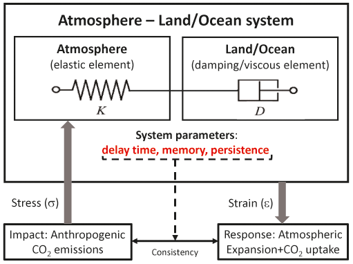
Figure 1Rheological model to capture the stress–strain behavior of the global atmosphere–land and ocean system as a Maxwell body consisting of elastic (atmosphere) and damping (land–ocean) elements. The stress (in units of Pa; known) is given by the carbon (CO2) emissions from fossil fuel burning and land use, while the strain (in units of 1; assumed exponential, otherwise unknown) is given by the expansion of the atmosphere by volume and uptake of CO2 by sinks. Independent estimates of K and D, the compression and damping characteristics of the MB, allow its stress–strain behavior to be captured and adjusted until consistency is achieved (see text).
In practice, rheology is principally concerned with extending continuum mechanics to characterize the flow of materials that exhibit a combination of elastic, viscous, and plastic behavior (that is, including hereditary behavior) by properly combining elasticity and (Newtonian) fluid mechanics. Limits (e.g., viscosity limits) exist beyond which basic rheological models are recommended to be refined. However, these limits are fluent, and basic rheological models also produce useful results beyond these limits (Malkin and Isayev, 2017; Mezger, 2006; TU Delft, 2022).
The mathematical treatment of an MB is standard. Depending on whether the strain (ε) or the stress (σ) is known (in addition to the compression and damping characteristics K and D), the stress–strain equation describing the MB between 0 and t can be applied in a stress-explicit form,
or in a strain-explicit form,
with σ(0) and ε(0) denoting initial conditions and a dot the derivative by time (Roylance, 2001; Bertram and Glüge, 2015).
Here, we focus on the application of these equations in an atmosphere–land and ocean carbon context. For an observer it is the overall strain response of that system (expansion of the atmosphere by volume and uptake of CO2 by sinks) that is unknown. However, since atmospheric CO2 concentrations have been observed to increase exponentially (quasi-continuously), the strain can be expected to be exponential or close to exponential. In addition, we provide independent estimates of the likewise unknown compression and damping characteristics of the MB. This a priori knowledge allows Eqs. (1a) and (1b) to be used stepwise in combination to narrow down our initial estimate of the ratio in particular. More accurate knowledge of this ratio is needed when we go beyond textbook knowledge by distilling three parameters – delay time (reflecting the temporal offset mentioned above), memory, and persistence – from the stress-explicit equation. The three parameters depend, ceteris paribus, solely on the system's characteristic ratio and allow deeper and novel insights into that system. We see the atmosphere–land and ocean system as being trapped progressively over time in terms of persistence. Given its reduced ability to build up memory, we expect system failures globally well before 2050 if the current trend in emissions is not reversed immediately and sustainably. Put differently, the stress–strain approach comes with its own internal limits which govern the behavior of the atmosphere–land and ocean carbon system independently from any external target values (such as temperature targets justified by means of global change research).
There is a wide range of other approaches which aim at exploring memory and persistence in Earth systems data, typically with the focus on individual Earth subsystems or processes (e.g., atmospheric temperature or carbon dioxide emissions). So far, applied approaches have mainly been based on classical time series and time–space analyses to uncover the memory or causal patterns contained in observational data (Barros et al., 2016; Belbute and Pereira, 2017; Caballero et al., 2002; Franzke, 2010; Lüdecke et al., 2013). However, these approaches come with well-known limitations which can all be attributed, directly or indirectly, to the issue of forecasting (more precisely, the conditions placed on the data to enable forecasting) or are not based on physics (Aghabozorgi et al., 2015; Darlington, 1996; Darlington and Hayes, 2016). By way of contrast, we do not forecast. We perpetuate long-term historical conditions which, in turn, allows the delay time in the atmosphere–land and ocean system to be expressed analytically in terms of memory and persistence. We are not aware of any scientific discipline or research area in which memory and persistence are defined other than statistically and are interlinked, if at all, other than via correlation.
Rheological approaches are common in Earth systems modeling as well. Typically, they are applied to mimic the long(er)-term behavior of Earth subsystems, e.g., its mantle viscosity, which is crucial for interpreting glacial uplift resulting from changes in planetary ice sheet loads (Müller, 1986; Whitehouse et al., 2019; Yuen et al., 1986). Yet, to the best of our knowledge, a rheological approach to unravel the memory and persistence behavior of the global atmosphere–land and ocean system in response to the long-lasting increase in atmospheric CO2 emissions had not been applied before.
We describe our rheological model (MB) approach in detail in Sect. 2, while we provide an overview of the applied data and conversion factors in Sect. 3. In Sect. 4 we describe how we derive first-order estimates of the main characteristics of the atmosphere–land and ocean system (in terms of the MB's K and D characteristics) by using available knowledge. Although uncertain, these estimates become useful in Sect. 5 where we apply the aforementioned stress- and strain-explicit equations to quantify delay time, memory, and persistence of the atmosphere–land and ocean system. We conclude by taking account of our main findings in Sect. 6.
This section provides an overview of how we process Eq. (1a) and how we distill delay time, memory, and persistence from this equation. To familiarize oneself with the details, the reader is referred to the Supplement.
To start with, we assume that we know the order of magnitude of both the ratio characteristic of the atmosphere–land and ocean system and the rate of change in the strain ε given by with the exponential growth factor α>0. These first-order estimates permit Eqs. (1a) and (1b) to be used stepwise in combination.
Equation (1a): we vary both and α to reproduce the known stress σ given by the CO2 emissions from fossil fuel burning (fairly well known) and land use (less known) (Global Carbon Project, 2019).
Equation (1b): we insert both the fine-tuned ratio and the known stress σ to compute the strain ε and check its derivative by time.
We consider this procedure a check of consistency, not a proof of concept.
Delay time, memory, and persistence are characteristic (functions) of the MB. They are contained in the integral on the right side of Eq. (1a) and are defined independently of initial conditions. These appear only in the lower boundary of that integral, which allows initial conditions other than zero to be considered by taking advantage of the integral's additivity. Thus, without loss of generality, we rewrite Eq. (1a) for σ(0)=0, which results in
(see Supplement Information 1) where and . The term represents a time characteristic of the MB under (here) exponential strain (i.e., of the MB that responds to the stress acting upon it), whereas is the relaxation time of the MB (i.e., of the MB that relaxes unhindered after the stress causing that strain has vanished or that responds to strain held constant over time; also known as the relaxation test; Bertram and Glüge, 2015). However, to ensure that exponents still come in units of 1 after we split them up, we introduce the dimensionless time globally (which will be discretized in the sequel when we refer to a temporal resolution of 1 year and set Δt=1 yr) such that, for example, .
To understand the systemic nature of the MB, we explore its stress dependence on , which contains the ratio of K and D, the two characteristic parameters of the MB, by way of derivation by q (while α is held constant). To this end, we transform Eq. (2a) further to
and execute , the derivation by q of the system's rate of change σD (which is given in units of yr−1). Doing so allows (what we call) delay time T to be distilled (see Supplement Information 2). It is defined as
where qβ=qαq, , and . The delay time behaves asymptotically for increasing n and approaches . We further define
with , and
with as the MB's characteristic memory and persistence, respectively. As is commonly done, we keep the list of independent parameters minimal. (We only allow K and D – i.e., q – in addition to n; see Eqs. 2b and 3–5 in particular.)
T as given by Eq. (3) is not simply characteristic of the MB described by Eqs. (2a) and (2b); it can be shown to appear as delay time in the argument of any function dependent on current and previous times, with a weighting decreasing exponentially backward in time (see Supplement Information 3). Equation (4) reflects the history the MB was exposed to systemically prior to current time n (during which α was constant; see Supplement Information 4). Put simply, M can be understood as the depreciated (q-weighted) strain summed up backward in time. Equation (5) can be shortened to . If we assume that q can be changed in retrospect at n=0, this equation tells us that if T – that is, ΔM per Δq (or, likewise, per ; see the first part of Eq. 3) – is small, P is great because the change in the system's characteristics (contained in q) hardly influences the MB's past, with the consequence that the past exhibits a great path dependency, and vice versa. We therefore perceive persistence and path dependency as synonymous.
An additional quantity to monitor is ln (M⋅P), which approaches for increasing n, with as the characteristic rate of change in the MB. The ratio allows monitoring of how much the system's natural rate of change is exceeded as a consequence of the continued increase in stress (see Supplement Information 5).
A detailed overview of the carbon data and conversion factors used in this paper (and also by the carbon community) is given in Supplement Information 6. The data pertain to atmosphere, land, and oceans:
-
atmospheric CO2 concentration (in ppm);
-
CO2 emissions from fossil fuel combustion and cement production (in Pg C yr−1);
-
land use change emissions (in Pg C yr−1);
-
net primary production (in Pg C yr−1); and
-
dissolved organic carbon (in µmol kg−1).
They are given by source and time range and are also described briefly. The context within which they are used is revealed in each of the following sections. The conversion factors are standard; they are needed to convert C to CO2 and parts per million by volume (ppmv) CO2 to petagrams of carbon (Pg C) or pascal (Pa).
In this section we provide independent estimates of the damping and compression characteristics of the atmosphere–land and ocean system, with DL and DO denoting the damping constants assigned to land and oceans, respectively, and K denoting the compression modulus assigned to the atmosphere. We capture the characteristics' right order of magnitude only – which can be done on physical grounds by evaluating the combined (net) strain response of each subsystem on the grounds of increasing CO2 concentrations in the atmosphere. These first-order estimates are adequate as they allow sufficient flexibility for Sect. 5, where we narrow down our initial estimates by using Eqs. (1a) and (1b) stepwise in combination to achieve consistency.
4.1 Estimating the damping constant DL
Increasing concentrations of CO2 in the atmosphere trigger the uptake of carbon by the terrestrial biosphere. The intricacies of this process, including potential (positive and negative) feedback processes, are widely discussed (Dusza et al., 2020; Heimann and Reichstein, 2008; Smith, 2012). The crucial question is how we have observed the process of carbon uptake by the terrestrial biosphere taking place in the past. Compared to the reaction of the atmosphere to global warming (an expansion of the atmosphere by volume), we consider this process to be long(er) term in nature and perceive it as a Newton-like (damping) element.
Biospheric carbon uptake is described by the biotic growth factor:
which is used to approximate the fractional increase in net primary productivity (NPP) per unit increase in atmospheric CO2 concentration (Wullschleger et al., 1995; Amthor and Koch, 1996; Luo and Mooney, 1996). Here we make use of the model-derived NPP time series (1900–2016) provided by O'Sullivan et al. (2019) to calculate βb (O'Sullivan et al., 2019). To understand the uncertainty range underlying βb for 1959–2018, we use the photosynthetic beta factor:
where L is the so-called leaf-level factor denoting the relative leaf photosynthetic response to a 1 ppmv change in the atmospheric concentration of CO2, bounded by
(see below), and Ph is the global photosynthetic carbon influx (i.e., gross primary productivity). Equation (7) is similar to Eq. (6). In Eq. (6) βb represents biomass production changes in response to CO2 changes, whereas in Eq. (7) βPh describes photosynthesis changes in response to CO2 changes (Luo and Mooney, 1996).
L can be shown to be independent of plant characteristics, light, and the nutrient environment and to vary little by geographic location or canopy position. Thus, L is virtually a constant across ecosystems and a function of time-associated changes in atmospheric CO2 only (Luo and Mooney, 1996).
We use Eq. (7) to test whether βb falls within the range of βPh given by the quantifiable photosynthetic limits L1 (photosynthesis limited by electron transport) and L2 (photosynthesis limited by RuBisCO activity). Figure 2 shows the biotic growth factors from O'Sullivan et al. (2019) that consider changes in NPP due to the combined effect of CO2 fertilization, nitrogen deposition, climate change, and carbon–nitrogen synergy (βNPP_comb) as well as due to CO2 fertilization () only. For 1960–2016, βNPP_comb falls between β1:=βPh(L1) and β2:=βPh(L2), closer to β1 than to β2, whereas even falls below the lower β1 limit.
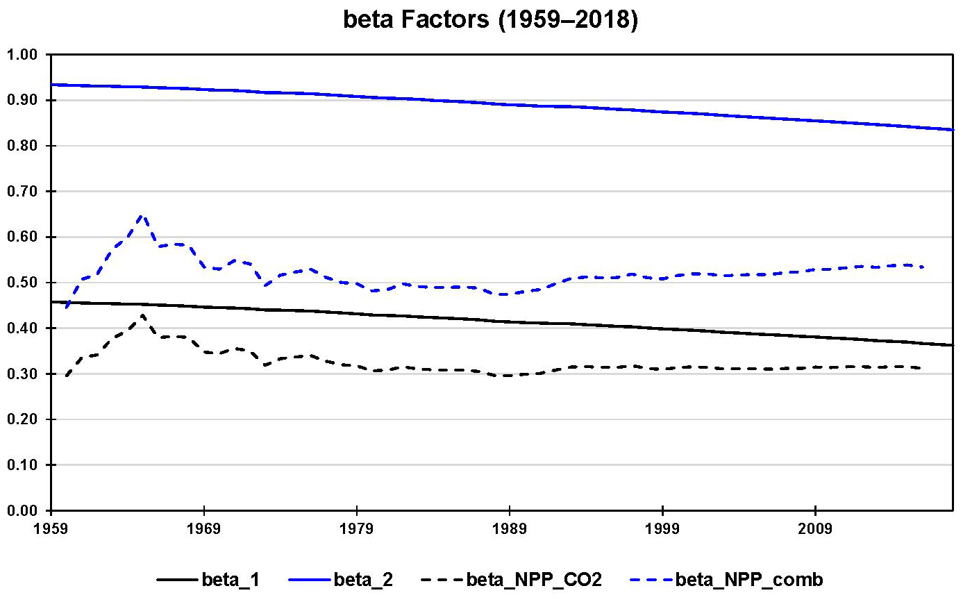
Figure 2Using the lower (β1) and upper (β2) limits of the photosynthetic beta factor to test the range of the biotic growth factor (βb) for 1960–2016. The biotic growth factor is derived with the help of modeled net primary production (NPP) values accounting for CO2 fertilization, nitrogen deposition, climate change, and carbon–nitrogen synergy. refers to O'Sullivan et al. (2019), who consider the change in NPP due to CO2 fertilization only, and βNPP_comb refers to the change in NPP due to the combined effect. All beta factors are in units of 1.
Rewriting Eq. (7) in the form
with Ph=120 Pg C yr−1 indicates that the additional amount of annual relative photosynthetic carbon influx, stimulated by a yearly increase in atmospheric CO2 concentration, can be estimated by Li or the sequence of Li if ΔCO2 spans multiple years (see Supplement Information 7 and Supplement Data 1). Plotting against time allows lower and upper slopes (rates of strain)
and
to be derived for 1959–2018. A linear fit works well in either case. The cumulative increase in atmospheric CO2 concentration since 1959, , exhibits a moderate exponential (close to linear) trend. Thus, plotting annual changes in CO2, normalized on the aforementioned rates of strain, versus time allows the remaining (moderate) trends to be interpreted alternatively, namely as average photosynthetic damping constants with appropriate uncertainty given by half the maximal range (see Fig. 3 and Supplement Data 1).
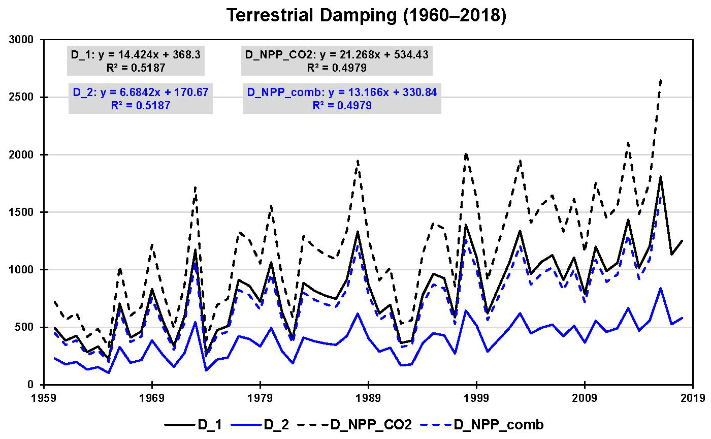
Figure 3Terrestrial carbon uptake perceived as damping (in ppmv yr) based on the limits of leaf photosynthesis (1960–2018: D1 and D2) and on model-derived changes in net primary production (NPP; 1960–2016) due to the combined effect of CO2 fertilization, nitrogen deposition, climate change, and carbon–nitrogen synergy (DNPP_comb) as well as CO2 fertilization only (). The linear trends of the four damping series are shown at the top. These are used to interpret damping as constants with appropriate uncertainty (given by half the maximal range).
Repeating the same procedure for 1959–2016 with O'Sullivan et al. (2019) model-derived NPP values considering the change in NPP due to CO2 fertilization as well as the total change in NPP, we find
and
(linear fits still work well), and consequently
As before, these estimates are closer to the lower leaf-level factor (higher photosynthetic D) than to the higher leaf-level factor (lower photosynthetic D; Fig. 3).
Here we interpret the O'Sullivan et al. (2019) Earth systems model as a typical one, which means that the NPP changes it produces are common. We therefore (and sufficient for our purposes) choose the damping constant D1 as a good estimator in light of the total change in NPP of the terrestrial biosphere since 1960. Hence,
DL is on the order of viscosity indicated for bitumen and asphalt (Mezger, 2006).
4.2 Estimating the damping constant DO
Increasing concentrations of CO2 in the atmosphere trigger the uptake of carbon by the oceans (National Oceanic and Atmospheric Administration, 2015). Like the uptake of carbon by the terrestrial biosphere, we consider this process to behave like a Newton (damping) element in our MB because of the de facto irreversibility on the shorter timescale we are interested in (Schwinger and Tjiputra, 2018).
The Revelle (buffer) factor (R) quantifies how much atmospheric CO2 can be absorbed by homogeneous reaction with seawater. R is defined as the fractional change in CO2 relative to the fractional change in dissolved inorganic carbon (DIC):
(Here, in contrast to before, atmospheric CO2 is referred to in units of µatm and therefore indicated by pCO2.) An R value of 10 indicates that a 10 % change in atmospheric CO2 is required to produce a 1 % change in the total CO2 content of seawater (Bates et al., 2014; Egleston et al., 2010; Emerson and Hedges, 2008).
DIC and R have been observed at seven ocean carbon time series sites for periods from 15 to 30 years (between 1983 and 2012) to change slowly and linearly with time (Bates et al., 2014):
(see also Supplement Data 2). Here it is sufficient to proceed with spatiotemporal averages. As before, the cumulative increase in atmospheric CO2 concentration since 1983, , exhibits a moderate exponential (close to linear) trend. Thus, plotting annual changes in pCO2, normalized on the rates of strain , versus time allows the remaining (moderate) trend to be interpreted alternatively, namely as an average oceanic damping constant with appropriate uncertainty given by half the maximal range (see Fig. 4 and Supplement Data 2):
DO is on the order of viscosity indicated for bitumen and asphalt, yet approximately 3.7 times greater than DL.
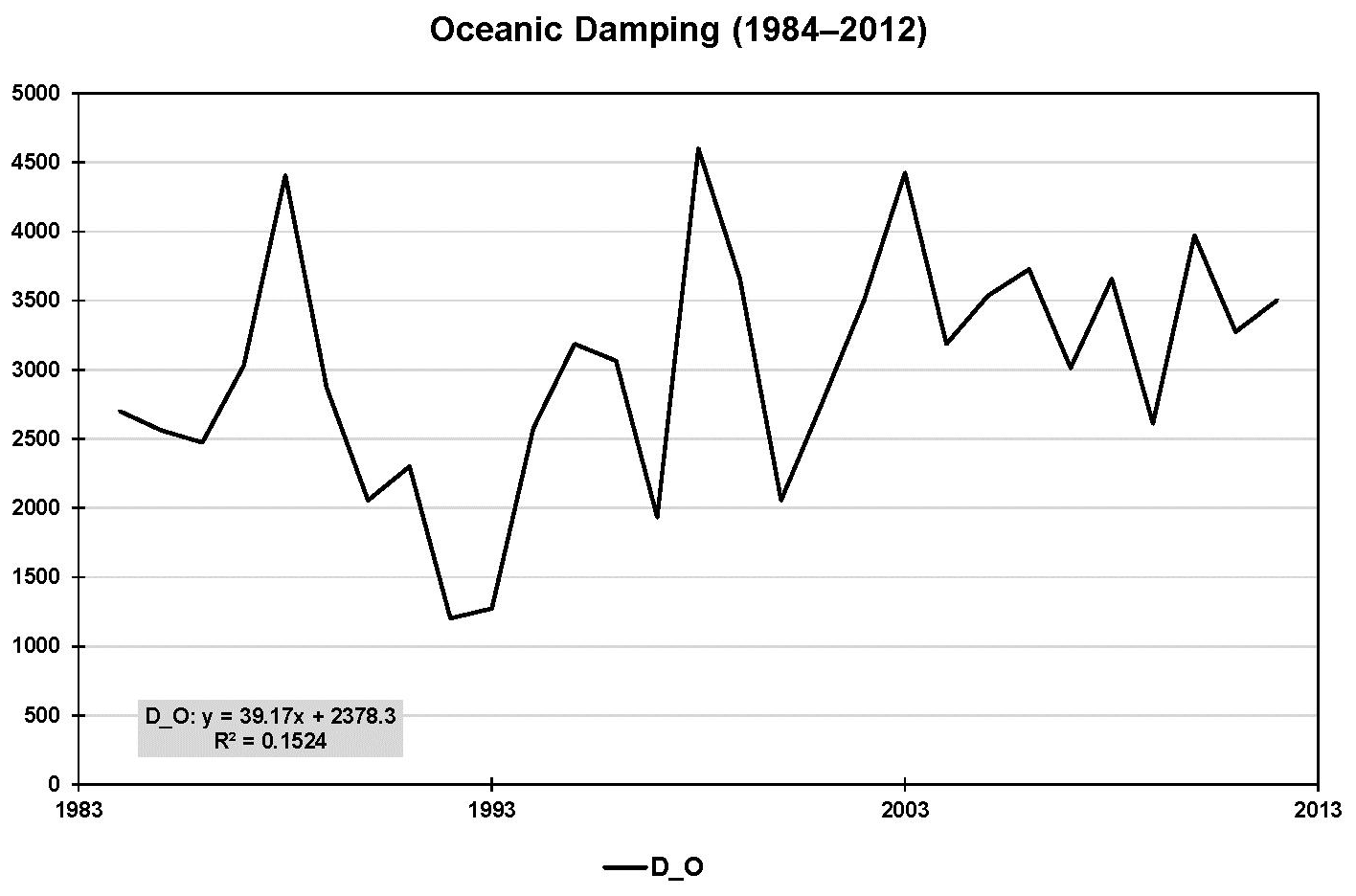
Figure 4Oceanic carbon uptake perceived as damping (in ppmv yr) based on observations at seven ocean carbon time series sites for periods from 15 to 30 years (between 1983 and 2012). The linear trend in oceanic damping, shown at the bottom, is used to interpret damping as a constant with appropriate uncertainty (given by half the maximal range).
4.3 Estimating the compression modulus K
The long-lasting increase in GHG emissions has caused the CO2 concentration in the atmosphere to increase and the atmosphere as a whole to warm (with tropospheric warming outstripping stratospheric cooling) and to expand (in the troposphere by approximately 15–20 m per decade since 1990) (Global Carbon Project, 2019; Lackner et al., 2011; Philipona et al., 2018; Steiner et al., 2011, 2020). Our whole-subsystem (net-warming) view does not invalidate the known facts that CO2 in the atmosphere is well-mixed (except for very low altitudes at which deviations from uniform CO2 concentrations are caused by the dynamics of carbon sources and sinks) and that the volume percentage of CO2 in the atmosphere stays almost constant up to high altitudes (Abshire et al., 2010; Emmert et al., 2012).
Compared to the slow uptake of carbon by land and oceans, we assume the atmosphere to be represented well by a Hooke element in the MB and this to serve as a (sufficiently stable) surrogate physical descriptor for the reaction of the atmosphere as a whole (Sakazaki and Hamilton, 2020). However, in the case of a gas, Young's modulus E must be replaced by the compression modulus K, the reciprocal of which is compressibility κ. Both K and κ scale with altitude, which we get to grips with in the following. Compressibility is defined by
(κ>0) (OpenStax, 2020). Depending on whether the compression happens under isothermal or adiabatic conditions, the compressibility is distinguished accordingly. It is defined by
in the isothermal case and
in the dry adiabatic case, in which γ is the isentropic coefficient of expansion. Its value is 1.403 for dry air (1.310 for CO2) under standard temperature (273.15 K) and pressure (1 atm; 101.325 kPa) (Wark, 1983). We consider a carbon-enriched atmosphere to also be air.
However, the observed expansion of the troposphere happens neither isothermally nor dry adiabatically but polytropically. Moreover, our ignorance of the exact value of κ is overshadowed by the uncertainty in altitude – or top of the atmosphere (TOA) – which we need as a reference for κ (thus K). As a matter of fact, there is considerable confusion as to which altitude the TOA refers to in climate models (CarbonBrief, 2018; NASA Earth Observatory, 2006).
To advance, we refer to the (dry adiabatic) standard atmosphere, which assigns a temperature gradient of −6.5 ∘C per 1000 m up to the tropopause at 11 km, a constant value of −56.5 ∘C (216.65 K) above 11 km and up to 20 km, and other gradients and constant values above 20 km (Cavcar, 2000; Mohanakumar, 2008). Guided by the distribution of atmospheric mass by altitude, we choose the stratopause as our TOA (at about 48 km of altitude and 1 hPa), with uncertainty ranging from middle to higher stratosphere (at about 43 km of altitude and 1.9 hPa) to mid-mesosphere (at about 65 km of altitude and 0.1 hPa) (Digital Dutch, 1999; International Organization for Standardization, 1975; Mohanakumar, 2008; Zellner, 2011). We assign the resulting uncertainty of 90 % in relative terms to
which we consider sufficiently large to compensate for the unknown isentropic coefficient in the first place; that is,
For comparison, Kad ranges from 400 to 412 hPa were the TOA allocated within the troposphere (exhibiting, for the reference used here, an expansion of 20 m; see Supplement Information 8).
Equations (1a) (or 2a) and (1b) are used stepwise in combination to conduct three sets of stress–strain experiments including sensitivity experiments (SEs):
A. for the period 1959–2015 assuming zero stress and strain in 1959,
B. for the period 1959–2015 assuming zero stress and strain in 1900, and
C. for the period 1959–2015 assuming zero stress and strain in 1850
and, ultimately, also before 1850 (i.e., zero anthropogenic stress before that date).
The logic of the experiments is determined by both the availability of data (see Supplement Information 6) and the increasing complementarity from A to C (see below). The basic procedure is always the same. We insert into Eq. (1a) our first-order estimates of Pa yr and Pa yr: that is, Pa yr, and Pa. At the same time, we use the growth factor αppm=0.0043 yr−1, which reflects the exponential increase in the CO2 concentration in the atmosphere between 1959 and 2018 (see Supplement Data 1) as our first-order estimate for α in , the rate of change in strain ε. We apply Eq. (1a) by varying both and α to reproduce the known stress σ on the left, given by the CO2 emissions from fossil fuel burning and land use. To restrict the number of variation parameters to two, we let K and D deviate from their respective mean values equally in relative terms (i.e., we assume that our first-order estimates exhibit equal inaccuracy in relative terms) and express α as a multiple of αppm. This is easily possible with the introduction of suitable factors (see Supplement Data 3) that allow σ to be reproduced quickly and with sufficient accuracy. The main reason this works well is that the two factors pull the two exponential functions on the right side of Eq. (2a) – and (), which determine the quality of the fit – in different directions.
To A
This is our set of reference experiments, all for the period 1959–2015. This set comprises A.1 (a stress-explicit experiment), A.2 (three strain-explicit experiments), and A.3 (SEs expanding the strain-explicit experiments). The parameters α, λ, and λβ are reported in units of yr−1, as is commonly done.
To A.1
In this experiment we vary the ratio (λ in Table 1) and α to reproduce the monitored stress σ(t) on the left side of Eq. (2a) (see Supplement Data 3). This tuning process (hereafter referred to as Case 0) allows us to test whether K and D, in particular, stay within their estimated limits, namely, Pa, and Pa yr or, equivalently, yr−1. Column “Case 0” in Table 1 indicates that this case is practically identical to choosing , the smallest ratio deemed possible. For Case 0 we find K=9.9 Pa and D=461.5 Pa yr (thus, yr−1) as well as, concomitantly, α=0.0247 yr−1 (thus, yr−1).
Table 1Overview of parameters in experiments A.1–A.3.
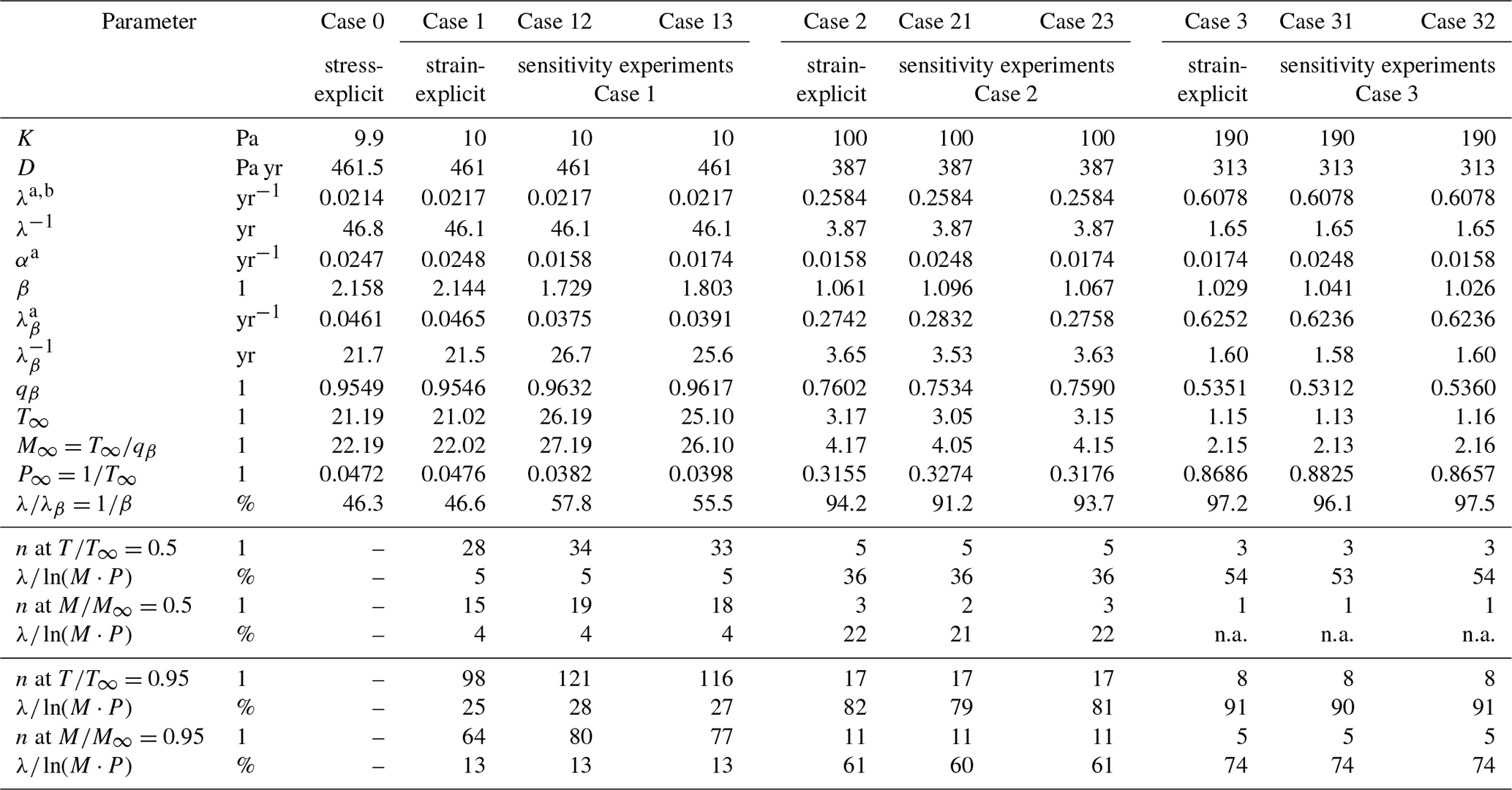
a Given per year (yr−1). b Derived for K and D deviating from their respective mean values equally in relative terms. The notation “n.a.” stands for not assessable.
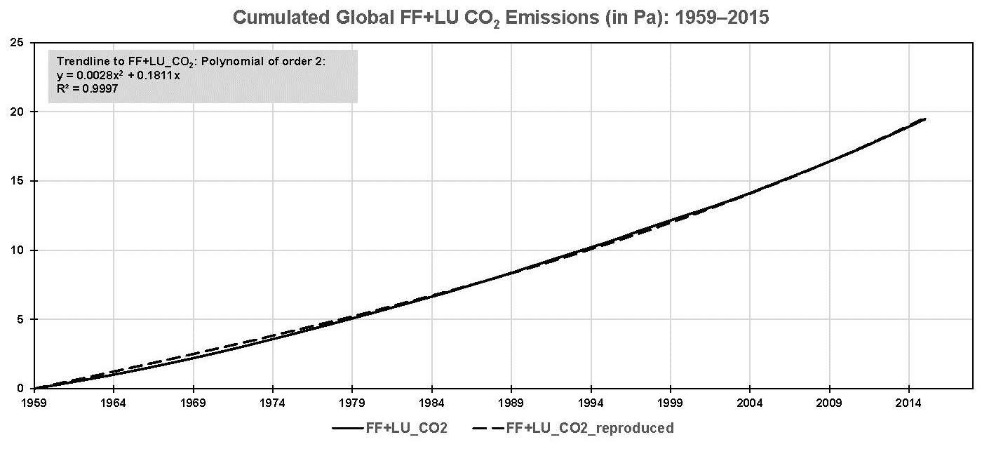
Figure 5Case 0: and α on the right side of Eq. (2a) are tuned to reproduce the stress σ(t) on the left side of that equation, given by the monitored (but cumulated) CO2 emissions from fossil fuel burning and land use activities (in Pa). The value resulting for complies with its lower limit deemed possible based on the uncertainties derived for K and D in Sect. 4.
Figure 5 reflects the result of the tuning process graphically. It shows how well the monitored stress, given by the cumulated CO2 emissions from fossil fuel burning and land use activities since 1959, can be reproduced by Eq. (2a). The quality of the tuning is observed by summing the squares of differences between monitored and reproduced stress from 1959 to 2015 using the SUMXMY2 command in Excel. (We stopped the tuning process with the sum at about 1.400 Pa2 when changes in K and D became negligible, resulting in a correlation coefficient of 0.9998; see Supplement Data 3.)
Figure 5 also shows the parameters needed to describe the monitored stress by a second-order polynomial regression (see the grey box in the upper left corner of the figure). We have not yet used this regression but will do so in the strain-explicit experiments described next.
To A.2
We use Eq. (1b) with and , the second-order polynomial regression of the monitored stress (see Fig. 5), to conduct three experiments (hereafter referred to as Cases 1–3) to explore the spread in the strain ε. To this end, we let the ratio vary from minimum (Case 1) to mean (Case 2) to maximum (Case 3; see Table 1 and Supplement Data 4) irrespective of the outcome of the Case 0 experiment, which suggests that compared to Cases 2 and 3, Case 1 (K minimal: the atmosphere is rather compressible; D maximal: the uptake of carbon by land and oceans is rather viscous) appears to be more in conformity with reality than Cases 2 and 3.
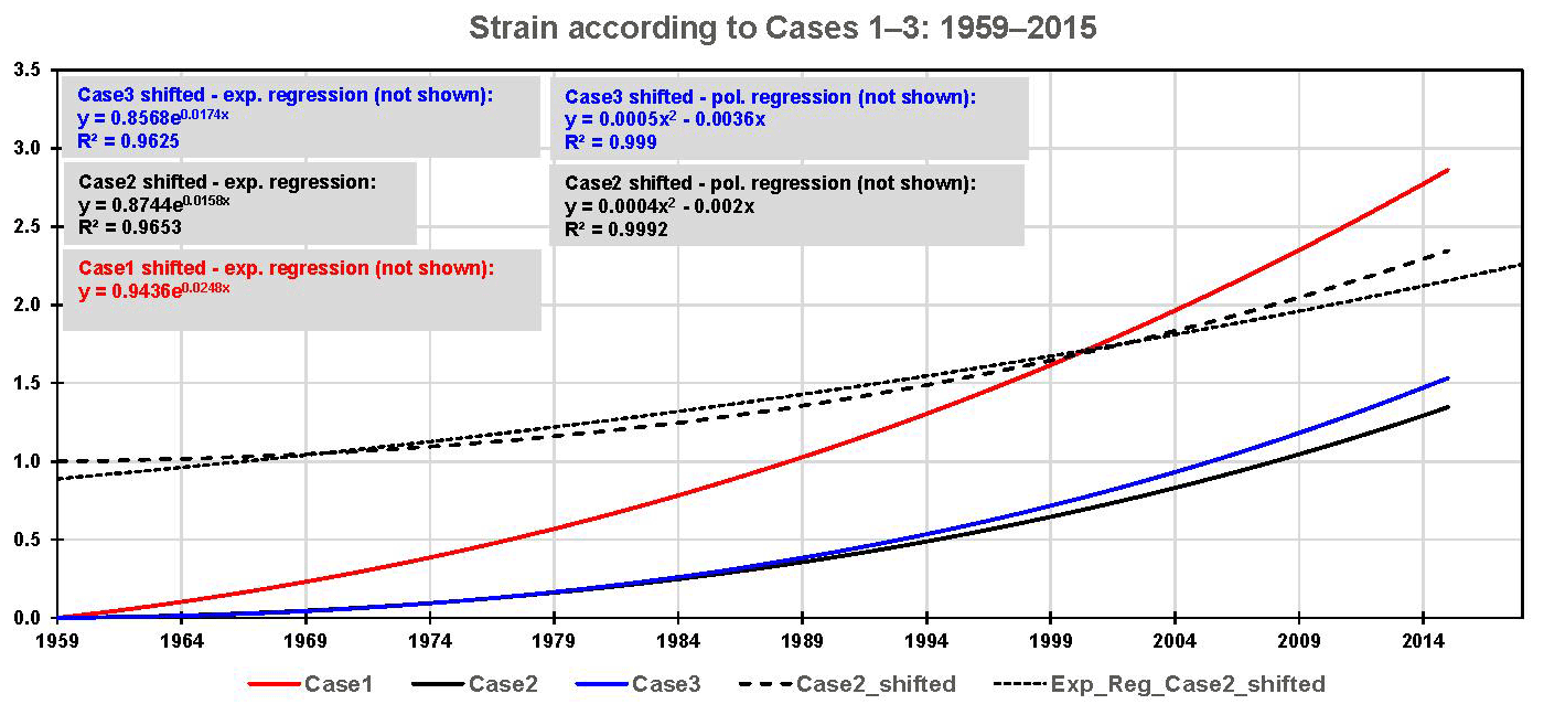
Figure 6Cases 1–3: the ratio is varied from minimum (Case 1: solid red) to mean (Case 2: solid black) to maximum (Case 3: solid blue) to explore the spread in the strain ε (in units of 1) on the left side of Eq. (1b), while the monitored stress is described by a second-order polynomial (see the text). These strain responses have to be shifted upward (so that they pass through 1 in 1959) to derive their rates of change if described by an exponential regression (here only demonstrated for Case 2). As is already illustrated in Case 0, the exponential regression in Case 1 is excellent (see the text), whereas second-order polynomial regressions provide better fits in Cases 2 and 3 (see the boxes in the figure; the polynomial regressions are not shown).
Figure 6 reflects these experiments graphically. It shows that the range of strain responses is encompassed by Case 1 ( yr−1) and Case 2 ( yr−1) but not by Case 1 and Case 3 ( yr−1) – the solid blue line (Case 3) falls between the solid red (Case 1) and solid black (Case 2) lines – resulting from how K and D dominate the individual parts of Eq. (1b). These strain responses have to be shifted upward (so that they pass through 1 in 1959) to describe them by an exponential regression and to derive their rates of change. The exponential fit is excellent only in Case 1, as already illustrated in Case 0 (Case 0: λ=0.0214 yr−1, Case 1: λ=0.0217 yr−1), but inferior to the polynomial regressions, here of the second order, in Cases 2 and 3. However, a second-order polynomial approach to the strain has to be discarded because the stress derived with the help of Eq. (1a) would exhibit a linear behavior with increasing time and not be a polynomial of the second order as in Fig. 6 (see Supplement Information 9).
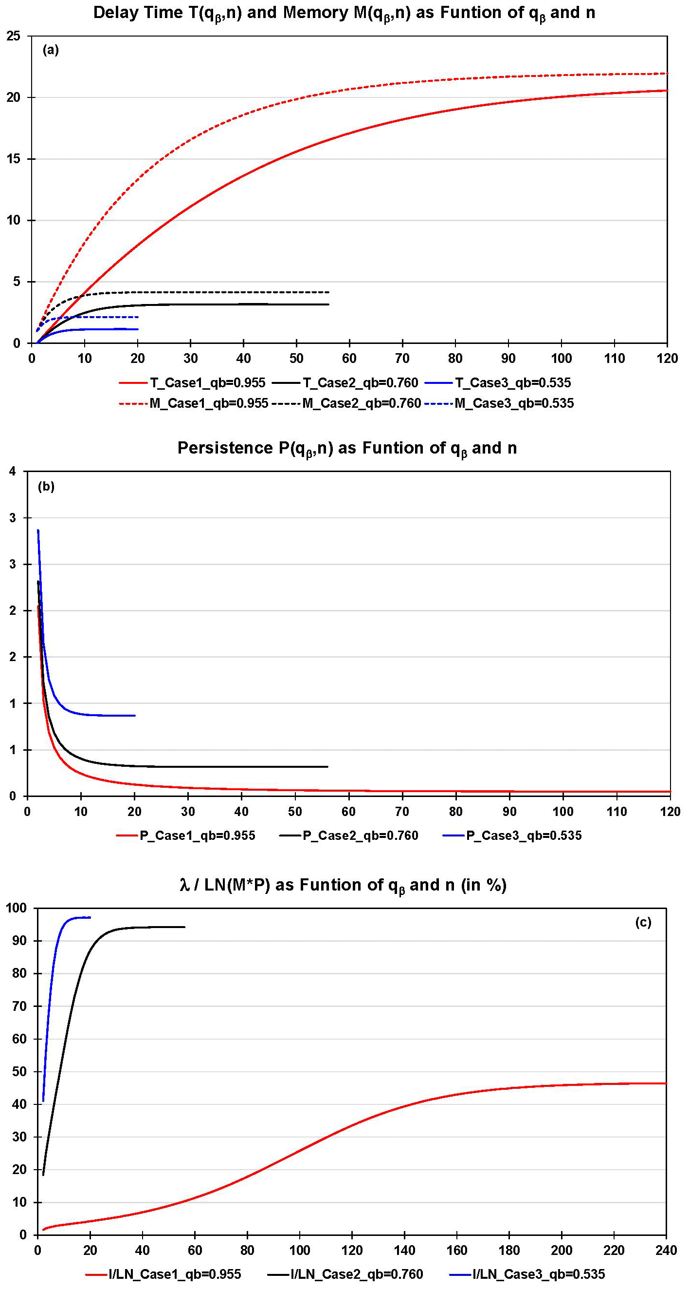
Figure 7Cases 1–3: (a) delay time T and memory M (in units of 1), (b) persistence P (in units of 1), and (c) the ratio (in %); all are versus time (in units of 1) as of n=0 (1959).
In this regard we note that a more targeted way forward would be to use a piecemeal approach. This approach requires the data series to be sliced into shorter time intervals, during which an exponential fit for the strain (which we assume to hold in principle in deriving Eq. 2a here) is sufficiently appropriate. Fortunately, as the SEs in A.3 indicate, we can hazard the consequences of using suboptimal growth factors resulting from suboptimal exponential regressions for the strain.
Equations (3) to (5) are used to determine delay time T, memory M, and persistence P (in units of 1) for Cases 1–3 as well as their characteristic limiting values T∞, M∞, and P∞ (see Table 1 and Supplement Data 5 to 8). We recall that T, M, and P are characteristic functions of the MB and are defined independently of initial conditions; these only specify the reference time for n=0 (here 1959). Figure 7a and b reflect the behavior of T, M, and P over time (in units of 1). For a better overview, Table 1 lists the times when these parameters exceed 50 % or 95 % of their limiting values (without indicating whether these levels go hand in hand with, e.g., global-scale ecosystem changes of equal magnitude). In the table we also specify the ratio for each of these times (see also Fig. 7c). The ratio approaches for n→∞ and indicates (as a percentage) how much smaller the system's natural rate of change in the numerator turns out to be compared to the system's rate of change in the denominator under the continued increase in stress. As is illustrated, in particular by Case 1 in the figure, the ratio does not increase at a constant pace as n increases, which shows the nonlinear strain response of the atmosphere–land and ocean system.
To A.3
Three sets of SEs serve to assess the influence of the exponential growth factor on the strain-explicit experiments described above.
SE1: α1=0.0248 yr−1 as in Case 1 (see Fig. 6) is also used in Cases 2 and 3 (hereafter referred to as Cases 21 and 31).
SE2: α2=0.0158 yr−1 as in Case 2 (see Fig. 6) is also used in Cases 1 and 3 (hereafter referred to as Cases 12 and 32).
SE3: α3=0.0174 yr−1 as in Case 3 (see Fig. 6) is also used in Cases 1 and 2 (hereafter referred to as Cases 13 and 23).
Table 1 shows that the influence of a change in the exponential growth factor is small vis à vis the dominating influence of K and D and the quality in the estimates of T, M, and P. For instance, the dimensionless time n at ranges from 15 to 19 in Case 1 and experiments related to Case 1 (small persistency) and from 2 to 3 in Case 2 and experiments related to Case 2 (great persistency); in Case 3 and experiments related to Case 3, it does not exhibit a range at all (n≈1; very great persistency). These ranges for n tell us how long it takes to build up 50 % of the memory with time running as of n=0 (1959).
Table 2Cases 1–3 and related experiments: build-up of memory (%) as of n=0 (1959).
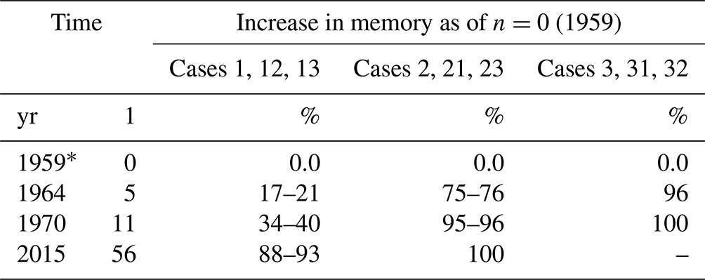
* Start year: .
Alternatively, we can ask how much memory has been built up until a given year. Table 2 tells us that after 56 years (i.e., in 2015) memory is still building up only in Case 1 and experiments related to Case 1, which means that the system still responds in its own characteristic way (as a result of a small K and a great D) to the continuously increasing stress; this is not so in Cases 2 and 3 (and related experiments). In the latter two cases today's uptake of carbon by land and oceans happens de facto outside the system's natural regime and solely in response to the sheer, continuously increasing stress imposed on it, whereas in Case 1 and experiments related to Case 1 the limits of the natural regime are not yet reached. This interpretation of Cases 1–3 (and related experiments) does not depend on how much carbon the system already took up before 1959. M is additive and defined independently of initial conditions; these only specify 1959 as reference time for n=0. This means by implication that the current M value (or its perpetuation) is contained in the M value (or is part of that value's perpetuation) which starts accruing from an earlier point in time (see also experiments B and C below).
Finally, it is important to note that it is prudent to expect that natural elements (like land and oceans) will not continue to maintain their damping (i.e., carbon uptake) capacity – or their capacity to embark on a, most likely, hysteretic downward path in the case of a sustained decrease in emissions – even well before they reach the limits of their natural regimes. They may simply collapse globally when reaching a critical threshold. We note that our choice of model binds us to the global scale and also does not allow “failure” to be specified further, e.g., with respect to when exactly a critical threshold will occur and in terms of whether carbon uptake decreases only or even ceases upon reaching the threshold.
To B and C
We report on the sets of stress–strain experiments B and C in combination. They can be understood as a repetition of the 1959–2015 Case 0 experiment (see A.1) but with the difference that now upstream emissions as of 1900 (B) or 1850 (C) are considered. This allows initial conditions for 1959 other than zero, as in the Case 0 experiment, to be considered (see Supplement Information 10 and Supplement Data 9 to 16).
Case 0: 1959–2015.
B: 1900–1958 (upstream emissions), 1959–2015.
C: 1850–1958 (upstream emissions), 1959–2015.
The experiments can be ordered consecutively in terms of time with the three 1959–2015 periods comprising a min–max interval to facilitate the drawing of a number of robust results in spite of the uncertainty underlying these stress–strain experiments (see Supplement Information 10). Between 1850 and 1959–2015 (i) the compression modulus K increased from ∼2 to 10–13 Pa (the atmosphere became less compressible), while (ii) the damping constant D decreased from ∼468 to 459–462 Pa yr (the uptake of carbon by land and oceans became less viscous), with the consequence that (iii) the ratio increased from ∼0.004–0.005 yr−1 to 0.021–0.028 yr−1 (i.e., by a factor of 4–6). Likewise, (iv) delay time T∞ decreased (hence, persistence P∞ increased) from ∼51 (∼0.02) to 18–21 (0.047–0.055), while (v) memory M∞ decreased from ∼52 to 19–22 on the dimensionless timescale.
Here we discuss our main findings in greater depth, recollect the assumptions underlying our global stress–strain approach, and conclude by returning to the three questions posed at the beginning.
We make use of an MB to model the stress–strain behavior of the global atmosphere–land and ocean carbon system and to simulate how humankind propelled that global-scale experiment historically, here as of 1850. The stress is given by the CO2 emissions from fossil fuel burning and land use, while the strain is given by the expansion of the atmosphere by volume and uptake of CO2 by sinks. The MB is a logical choice of stress–strain model given the uninterrupted increase in atmospheric CO2 concentrations since 1850.
The stress–strain model is unique and a valuable addendum to the suite of models (such as radiation transfer, energy balance, or box-type carbon cycle models), which are highly reduced but do not compromise complexity in principle. These models offer great benefits in safeguarding complex three-dimensional global change models. Here, too, the proposed stress–strain approach allows three system-characteristic parameters to be distilled from the stress-explicit equation – delay time, memory, and persistence – and new insights to be gained. What we consider most important is that these parameters come with their own internal limits, which govern the behavior of the atmosphere–land and ocean carbon system. These limits are independent from any external target values (such as temperature targets justified by means of global change research).
Knowing these limits is precisely the reason why we can advance the discussion and draw some preliminary conclusions. To start with, we look at the Case 0 experiment and the stress–strain experiments B and C in combination. The values of the Case 0 parameters T∞ and M∞, in particular, are at the upper end of the respective 1959–2015 min–max intervals (see Supplement Information 10). That is, the respective characteristic ratios and reach specified levels (e.g., 0.5 or 0.95; see Fig. 7a) slightly sooner than when T∞ and M∞ take on values at the lower end of the 1959–2015 min–max intervals. Given that Case 0 is well represented by Case 1, we can use the parameter values of the latter. According to column “Case 1” in Table 1, and reached their 0.5 levels after about 15- and 28-year-equivalent units on the dimensionless timescale (which was in 1974 and 1987), whereas they will reach their 0.95 levels after about 64- and 98-year-equivalent units (which will be in 2023 and 2057) – if the exponential growth factor α remains unchanged in the future.
This not unthinkable worst case provides a reference, as follows: we understand, in particular, the ability of a system to build up memory effectively as its ability to still respond to stress in its own characteristic way (i.e., within its natural regime). Therefore, it appears precautionary to prefer memory over delay time in avoiding potential system failures globally in the future. These we expect to happen well before 2050 if the current trend in emissions is not reversed immediately and sustainably. However, we reiterate that our choice of model binds us to the global scale and also does not allow failure to be specified further.
We consider our precautionary statement robust given both the uncertainties we dealt with in the course of our evaluation and the restriction of our variation parameters to two. One of the two variation parameters (λ) presupposes knowing K and D with equal inaccuracy in relative terms. This procedural measure in treating λ, in particular, offers a great applicational benefit but no serious restriction given that (while, ideally, α is constant) it is the ratio that matters and whose ultimate value is controlled by consistency – which comes in as a powerful rectifier. As a matter of fact, fulfilling consistency results in a ratio that ranges close to the lower uncertainty boundary which we deem adequate based on our preceding assessment. That means a smaller K, i.e., the atmosphere is more compressible than previously thought, and a greater D, i.e., the uptake of carbon by land and oceans is more viscous than previously thought (see Cases 1–3 in Table 1). However, the overall effect of the continued release of CO2 emissions since 1850 on the ratio is unambiguous – the ratio increased (see λ in Table SI10-2) by a factor of 4–6 (K increased: the atmosphere became less compressible; D decreased: the uptake of carbon by land and oceans became less viscous).
By way of contrast, persistence is less intelligible. Equation (5) allows persistence (as well as its systemic limit) to be followed quantitatively. However, it is conducive to understand persistence as path dependency and in qualitative terms, i.e., whether it increased or decreased. Thus, we see that P∞ increased since 1850 by a factor of 2–3 (see P∞ in Table SI10-2), which indicates that the atmosphere–land and ocean system is progressively trapped from a path dependency perspective. This, in turn, means that it will become progressively more difficult to (strain) relax the entire system (i.e., the atmosphere including land and oceans) – a mere 1-year decrease of a few percentage points in CO2 emissions, as reported recently for 2020, will have virtually no impact (Global Carbon Project, 2020).
To conclude, we return to the three questions posed in the beginning. These can be answered unambiguously.
Memory, just as persistence, is a characteristic (function) of the MB. Mathematically spoken, it is contained in the integral on the right side of Eq. (1a) and is defined independently of initial conditions. These appear only in the lower boundary of that integral, which allows initial conditions other than zero to be considered by taking advantage of the integral's additivity.
The memory of the atmosphere–land and ocean carbon system – Earth's memory – can be quantified. It can be understood as the depreciated strain summed up backward in time. We let memory extend backward in time to 1850, assuming zero anthropogenic stress before that date. Memory is measured in units of 1 and accrues continually over time (here as the result of the uninterrupted increase in stress).
Memory is constrained. It can be compared with a limited buffer, approximately 60 % of which humankind had already exploited prior to 1959 (see M∞ in Table SI10-2). We understand the effective build-up of memory as Earth's ability to still respond within its own natural stress–strain regime. However, this ability declines considerably with memory reaching high levels of exploitation (see in Table 1) – which we anticipate happening in the foreseeable future if CO2 emissions continue to increase globally as before.
Finally, we can also quantify the persistence of the atmosphere–land and ocean carbon system. It is also measured in units of 1. Persistence can be understood intuitively as path dependency and in qualitative terms. Concomitantly with the exploitation of memory, we see that P∞ increased since 1850 by approximately a factor of 2–3 – and can be expected to increase further if the release of CO2 emissions globally continues as before.
Based on these stress–strain insights we expect that the atmosphere–land and ocean carbon system will be forced outside its natural regime well before 2050 if the current trend in emissions is not reversed immediately and sustainably.
If terms or symbols are used in more than one way, we make them unambiguous by specifying (in parentheses) how they are used in the paper (e.g., CO2 as a chemical formula in the text or as a physical parameter in units of ppmv in mathematical equations). As a basic rule, physical parameters are always specified by their units.
| ad | adiabatic |
| C | carbon |
| comb | combined |
| CO2 | carbon dioxide (chemical formula) |
| CO2 | atmospheric CO2 concentration (in ppmv; |
| parameter) | |
| D | damping constant (in Pa yr) |
| DIC | dissolved inorganic carbon (in µmol kg−1) |
| E | Young's modulus (in Pa) |
| GHG | greenhouse gas |
| h | altitude (in m) |
| it | isothermal |
| K | compression modulus (in Pa) |
| L | land (index) |
| L | leaf-level factor (in ppmv−1; parameter) |
| M | memory (in units of 1) |
| MB | Maxwell body |
| n.a. | not assessable |
| NPP | net primary productivity and production |
| (in Pg C yr−1) | |
| O | oceans |
| p | atmospheric pressure (in hPa) |
| pCO2 | partial pressure of atmospheric |
| CO2 (in µatm) | |
| P | persistence (in units of 1) |
| Ph | global photosynthetic carbon influx |
| (in Pg C yr−1) | |
| q | auxiliary quantity (in units of 1) |
| R | Revelle (buffer) factor (in units of 1) |
| SD | supplementary data |
| SE | sensitivity experiment |
| SI | supplementary information |
| t | time (in yr) |
| T | delay time (in units of 1) |
| TOA | top of the atmosphere |
| w | weight(ed) |
| α | exponential growth factor of the strain |
| (in yr−1) | |
| αppm | exponential growth factor of the atmospheric |
| CO2 concentration (in yr−1) | |
| β | auxiliary quantity (in units of 1) |
| βb | biotic growth factor (in units of 1) |
| βPh | photosynthetic beta factor (in units of 1) |
| ε | strain (referring to atmospheric expansion by |
| volume and CO2 uptake by sinks; in units | |
| of 1) | |
| γ | isentropic coefficient of expansion (in units |
| of 1) | |
| κ | (in Pa−1) |
| σ | stress (atmospheric CO2 emissions from fossil |
| fuel burning and land use; in Pa) |
The article is supported by a Supplement provided by the authors. It consists of two parts, (1) Supplement Information (SI) and (2) Supplement Data (SD), and is available online at https://doi.org/10.22022/EM/06-2021.123 (Jonas et al., 2021).
The supplement related to this article is available online at: https://doi.org/10.5194/esd-13-439-2022-supplement.
MJ set up the physical model of the atmosphere–land and ocean system, derived its delay time, memory, and persistence, and provided the initial estimates of its compression and damping characteristics. RB contributed to the physical and mathematical improvement of the method and the physical consistency of results. IR and PZ contributed to the inspection of mathematical relations globally and their generalizations. PZ contributed to the strengthening of the method by evaluating alternative memory concepts known in mathematics.
Publisher's note: Copernicus Publications remains neutral with regard to jurisdictional claims in published maps and institutional affiliations.
Funding to facilitate collaboration between the Lviv Polytechnic National University and the International Institute for Applied Systems Analysis was provided by the Bilateral Agreement on Scientific and Technological Cooperation between the Cabinet of Ministers of Ukraine and the Government of the Republic of Austria (S & T Cooperation Project 10/2019; https://oead.at/en/, last access: 28 February 2022 and https://mon.gov.ua/eng, last access: 28 February 2022). Net primary production, land use change emission, and atmospheric expansion data were kindly provided personally by Michael O'Sullivan (University of Exeter), Julia Pongratz (Ludwig Maximilian University of Munich), and Andrea K. Steiner (Wegener Center for Climate and Global Change, Graz).
This research has been supported by the authors' home institutions, the International Institute for Applied Systems Analysis, and the Lviv Polytechnic National University.
This paper was edited by Zhenghui Xie and reviewed by Victor Brovkin and one anonymous referee.
Abshire, J. B., Riris, H., Allan, G. R., Weaver, C. J., Mao, J., Sun, X., Hasselbrack, W. E., Kawa, S. R., and Biraud, S.: Pulsed airborne lidar measurements of atmospheric CO2 column absorption, Tellus B, 62, 770–783, https://doi.org/10.1111/j.1600-0889.2010.00502.x, 2010. a
Aghabozorgi, S., Shirkhorshidi, A. S., and Wah, T. Y.: Time-series clustering – a decade review, Inform. Syst., 53, 16–38, https://doi.org/10.1016/j.is.2015.04.007, 2015. a
Amthor, J. S. and Koch, G. W.: Biota growth factor β: stimulation of terrestrial ecosystem net primary production by elevated atmospheric CO2, in: Carbon Dioxide and Terrestrial Ecosystems, edited by: Koch, G. W. and Mooney, H. A., Academic Press, San Diego, USA, 399–414, ISBN 0-12-505295-2, 1996. a
Barros, C. P., Gil-Alana, L. A., and Perez de Gracia, F.: Stationarity and long range dependence of carbon dioxide emissions: evidence for disaggregated data, Environ. Resour. Econ., 63, 45–56, https://doi.org/10.1007/s10640-014-9835-3, 2016. a
Bates, N. R., Astor, Y. M., Church, M. J., Currie, K., Dore, J. E., González-Dávila, M., Lorenzoni, L., Muller-Karger, F., Olafsson, J., and Santana-Casiano, J. M.: A time-series view of changing ocean chemistry due to ocean uptake of anthropogenic CO2 and ocean acidification, Oceanography, 27, 126–141, https://doi.org/10.5670/oceanog.2014.16, 2014. a, b
Belbute, J. M., and Pereira, A. M.: Do global CO2 emissions from fossil-fuel consumption exhibit long memory? A fractional integration analysis, Appl. Econ., 4055–4070, https://doi.org/10.1080/00036846.2016.1273508, 2017. a
Bertram, A., and Glüge, R.: Festkörpermechanik: Einachsige Materialtheorie: Viskoelastizität: Der MAXWELL-Körper, Otto-von-Guericke University Magdeburg, Magdeburg, Germany, https://docplayer.org/11977674-Festkoerpermechanik-mit-beispielen-von-albrecht- bertram-von-rainer-gluege-otto-von-guericke-universitaet-magdeburg.html (last access: 28 February 2022), 2015. a, b
Boucher, O., Halloran, P. R., Burke, E. J., Doutriaux-Boucher, M., Jones, C. D., Lowe, J., Ringer, M. A., Robertson, E., and Wu, P.: Reversibility in an Earth system model in response to CO2 concentration changes, Environ. Res. Lett., 7, 24013, https://doi.org/10.1088/1748-9326/7/2/024013, 2012. a
Caballero, R., Jewson, S., and Brix, A.: Long memory in surface air temperature: Detection, modeling, and application to weather derivative valuation, Clim. Res., 21, 127–140, https://doi.org/10.3354/cr021127, 2002. a
CarbonBrief: Climate modelling, Q&A: How do climate models work?, https://www.carbonbrief.org/qa-how-do-climate-models-work (last access: 28 January 2022), 15 January 2018. a
Cavcar, M.: The international standard atmosphere (ISA), Anadolu University, Eskişehir, Turkey, 7 pp., http://fisicaatmo.at.fcen.uba.ar/practicas/ISAweb.pdf (last access: 28 February 2022), 2000. a
Darlington, R. B.: A regression approach to time-series analysis, Script, Cornell University, Ithaca, NY, USA, http://node101.psych.cornell.edu/Darlington/series/series0.htm (last access: 28 February 2022), 1996. a
Darlington, R. B., and Hayes, A. F.: Regression analysis and linear models: Concepts, Applications, and Implementation, The Guilford Publications, New York, NY, USA, ISBN 978-1-4625-2113-5, 2016. a
Digital Dutch: 1976 Standard atmosphere calculator, https://www.digitaldutch.com/atmoscalc/ (last access: 28 January 2022), 1999. a
Dusza, Y., Sanchez-Cañete, E. P., Le Galliard, J.-F., Ferrière, R., Chollet, S., Massol, F., Hansart, A., Juarez, S., Dontsova, K., van Haren, J., Troch, P., Pavao-Zuckerman, M. A., Hamerlynck, E., and Barron-Gafford, G. A.: Biotic soil-plant interaction processes explain most of hysteric soil CO2 efflux response to temperature in cross-factorial mesocosm experiment, Sci. Rep., 10, 905, https://doi.org/10.1038/s41598-019-55390-6, 2020. a, b
Egleston, E. S., Sabine, C. L., and Morel, F. M. M.: Revelle revisited: buffer factors that quantify the response of ocean chemistry to changes in DIC and alkalinity, Global Biochem. Cy., 24, GB1002, https://doi.org/10.1029/2008GB003407, 2010. a
Emerson, S. and Hedges, J.: Chemical Oceanography and the Marine Carbon Cycle, Cambridge University Press, Cambridge, NY, USA, https://slideplayer.com/slide/9820843/ (last access: 28 February 2022), 2008. a
Emmert, J. T., Stevens, M. H., Bernath, P. F., Drob, D. P., and Boone, C. D.: Observations of increasing carbon dioxide concentration in Earth's thermosphere, Nat. Geosci., 5, 868–871, 2012. a
Flato, G., Marotzke, J., Abiodun, B., Braconnot, P., Chou, S. C., Collins, W., Cox, P., Driouech, F., Emori, S., Eyring, V., Forest, C., Gleckler, P., Guilyardi, E., Jakob, C., Kattsov, V., Reason, C., and Rummukainen, M.: Evaluation of climate models, in: Climate Change 2013: The Physical Science Basis, Contribution of Working Group I to the Fifth Assessment Report of the Intergovernmental Panel on Climate Change, edited by: Stocker, T. F., Qin, D., Plattner, G.-K., Tignor, M., Allen, S. K., Boschung, J., Nauels, A., Xia, Y., Bex, V., and Midgley, P. M., Cambridge University Press, Cambridge, UK, 741–866, ISBN 978-1-107-66182-0, https://www.ipcc.ch/site/assets/uploads/2018/02/WG1AR5_Chapter09_FINAL.pdf (last access: 28 February 2022), 2013. a
Franzke, C.: Long-range dependence and climate noise characteristics of Antarctic temperature data, J. Climate, 23, 6074–6081, https://doi.org/10.1175/2010JCLI3654.1, 2010. a
Garbe, J., Albrecht, T., Levermann, A., Donges, J. F., and Winkelmann, R.: The hysteresis of the Antarctic ice sheet, Nature, 585, 538–544, https://doi.org/10.1038/s41586-020-2727-5, 2020. a
Global Carbon Project: Global carbon budget 2019, https://www.icos-cp.eu/science-and-impact/global-carbon-budget/2019 (last access: 28 February 2022), 4 December 2019. a, b, c, d, e
Global Carbon Project: Carbon budget 2020, https://www.icos-cp.eu/science-and-impact/global-carbon-budget/2020 (last access: 28 February 2022), 11 December 2020. a
Harman, I. N. and Trudinger, C. M.: The simple carbon-climate model: SCCM7, CAWCR Technical Report No. 069, ISBN 9781486302628, https://www.cawcr.gov.au/technical-reports/CTR_069.pdf (last access: 28 February 2022), 2014. a
Heimann, M. and Reichstein, M.: Terrestrial ecosystem carbon dynamics and climate feedbacks, Nature, 451, 289–292, https://doi.org/10.1038/nature06591, 2008. a
International Organization for Standardization: Standard atmosphere, ISO 2533:1975, background source to https://en.wikipedia.org/wiki/International_Standard_Atmosphere (last access: 28 January 2022), 1975. a
Jonas, M., Bun, R., Ryzha, I., and Żebrowski, P.: Supplementary Material to Quantifying Memory and Persistence in the Atmosphere–Land/Ocean Carbon System, IIASA [data set], https://doi.org/10.22022/EM/06-2021.123, 2021. a
Lackner, B. C., Steiner, A. K., Hegerl, G. C., and Kirchengast, G.: Atmospheric climate change detection by radio occultation using a fingerprinting method, J. Climate, 24, 5275–5291, https://doi.org/10.1175/2011JCLI3966.1, 2011. a, b
Lüdecke, H. J., Hempelmann, A., and Weiss, C. O.: Multi-periodic climate dynamics: spectral analysis of long-term instrumental and proxy temperature records, Clim. Past, 9, 447–452, https://doi.org/10.5194/cp-9-447-2013, 2013. a
Luo, Y. and Mooney, H. A.: Stimulation of global photosynthetic carbon influx by an increase in atmospheric carbon dioxide concentration, in: Carbon Dioxide and Terrestrial Ecosystems, edited by: Koch, G. W. and Mooney, H. A., Academic Press, San Diego, USA, 381–397, ISBN 0-12-505295-2, 1996. a, b, c
Malkin, A. Ya., and Isayev, A. I.: Rheology: Concepts, Methods, and Applications, ChemTech Publishing, Toronto, Canada, 2017. a
Mezger, T. G.: The Rheology Handbook, Vincentz Network, Hannover, Germany, ISBN 3-87870-174-8, 2006. a, b
Mohanakumar, K.: Structure and composition of the lower and middle atmosphere, in: Stratosphere Troposphere Interactions, Springer, 1–53, https://doi.org/10.1007/978-1-4020-8217-7_1, 2008. a, b
Müller, G.: Generalized Maxwell bodies and estimates of mantle viscosity, Geophys. J. Int., 87, 1113–1141, https://doi.org/10.1111/j.1365-246X.1986.tb01986.x, 1986. a
NASA Earth Observatory: The top of the atmosphere, https://earthobservatory.nasa.gov/images/7373/the-top-of-the-atmosphere (last access: 28 January 2022), 2006. a
National Oceanic and Atmospheric Administration: Science on a sphere: ocean-atmosphere CO2 exchange, NOAA Global Systems Division, Boulder, CO, USA, https://sos.noaa.gov/datasets/ocean-atmosphere-co2-exchange/ (last access: 28 January 2022), 2015. a
OpenStax: Stress, strain, and elastic modulus (Part 2), https://phys.libretexts.org/@go/page/6472 (last access: 28 January 2022), 5 November 2020. a
O'Sullivan, M., Spracklen, D. V., Batterman, S. A., Arnold, S. R., Gloor, M., and Buermann, W.: Have synergies between nitrogen deposition and atmospheric CO2 driven the recent enhancement of the terrestrial carbon sink? Global Biogeochem. Cy., 33, 163–180, https://doi.org/10.1029/2018GB005922, 2019. a, b, c, d, e, f
Philipona, R., Mears, C., Fujiwara, M., Jeannet, P., Thorne, P., Bodeker, G., Haimberger, L., Hervo, M., Popp, C., Romanens, G., Steinbrecht, W., Stübi, R., and Van Malderen, R.: Radiosondes show that after decades of cooling, the lower stratosphere is now warming, J. Geophys. Res.-Atmos., 123, 12509–12522, https://doi.org/10.1029/2018JD028901, 2018. a, b
Roylance, D.: Engineering viscoelasticity, Massachusetts Institute of Technology, Cambridge, MA, USA, http://web.mit.edu/course/3/3.11/www/modules/visco.pdf (last access: 28 February 2022), 24 October 2001. a, b
Sakazaki, S., and Hamilton, K.: An array of ringing global free modes discovered in tropical surface pressure data, J. Atmos. Sci., 77, 2519–2530, https://doi.org/10.1175/JAS-D-20-0053.1, 2020. a
Schwinger, J. and Tjiputra, J.: Ocean carbon cycle feedbacks under negative emissions, Geophys. Res. Lett., 45, 5062–5070, https://doi.org/10.1029/2018GL077790, 2018. a, b
Smith, P.: Soils and climate change, Curr. Opin. Environ. Sust., 4, 539–544, https://doi.org/10.1016/j.cosust.2012.06.005, 2012. a, b
Steiner, A. K., Lackner, B. C., Ladstädter, F., Scherllin-Pirscher, B., Foelsche, U., and Kirchengast, G.: GPS radio occultation for climate monitoring and change detection, Radio Sci., 46, RS0D24, https://doi.org/10.1029/2010RS004614, 2011. a, b
Steiner, A. K., Ladstädter, F., Randel, W. J., Maycock, A. C., Fu, Q., Claud, C., Gleisner, H., Haimberger, L., Ho, S.-P., Keckhut, P., Leblanc, T., Mears, C., Polvani, L. M., Santer, B. D., Schmidt, T., Sofieva, V., Wing, R., and Zou, C.-Z.: Observed temperature changes in the troposphere and stratosphere from 1979 to 2018, J. Climate, 33, 8165–8194, https://doi.org/10.1175/JCLI-D-19-0998.1, 2020. a, b
Steffen, W., Sanderson, A., Tyson, P., Jäger, J., Matson, P., Moore III, B., Oldfield, F., Richardson, K. Schellnhuber, H. J., Turner II, B. L., and Wasson, R. J.: Global Change and the Earth System: A Planet Under Pressure, Springer-Verlag, Berlin, Germany, ISBN 978-3-540-26594-8, http://www.igbp.net/publications/igbpbookseries/igbpbookseries/globalchangeandtheearthsystem2004.5.1b8ae20512db692f2a680007462.html (last access: 28 February 2022), 2004. a
Steffen, W., Richardson, K., Rockström, J., Cornell, S. E., Fetzer, I., Bennett, E. M., Biggs, R., Carpenter, S. R., de Vries, W., de Wit, C. A., Folke, C., Gerten, D., Heinke, J., Mace, G. M., Persson, L. M., Ramanathan, V., Reyers, B., and Sörlin, S.: Planetary boundaries: guiding human development on a changing planet, Science, 347, 6223, 1259855, https://doi.org/10.1126/science.1259855, 2015. a, b
TU Delft: Rheometer. Faculty of Civil Engineering and Geosciences, Delft, the Netherlands, https://www.tudelft.nl/en/ceg/about-faculty/departments/watermanagement/research/waterlab/equipment/rheometer, last access: 28 January 2022. a, b
UN Climate Change: The Paris Agreement, https://unfccc.int/process-and-meetings/the-paris-agreement/the-paris-agreement, last access: 28 January 2022. a
UN Sustainable Development Goals: The Sustainable Development Agenda, https://www.un.org/sustainabledevelopment/development-agenda/, last access: 28 January 2022. a
Wark, K.: Thermodynamics, McGraw2Hill, New York NY, United States of America, background source to http://homepages.wmich.edu/~cho/ME432/Appendix1_SIunits.pdf (last access: 28 January 2022), 1983. a
Whitehouse, P. L., Gomez, N. King, M. A., and Wiens, D. .: Solid Earth change and the evolution of the Antarctic Ice Sheet, Nat. Commun., 10, 503, https://doi.org/10.1038/s41467-018-08068-y, 2019. a
Wullschleger, S. D., Post, W. M., and King, A. W.: On the potential for a CO2 fertilization effect in forests: estimates of the biotic growth factor based on 58 controlled-exposure studies, in: Biotic Feedbacks in the Global Climatic System, edited by: Woodwell, G. M. and Mackenzie, F. T., Oxford University Press, New York NY, USA, 85–107, ISBN 0-19-508640-6, 1995. a
Yuen, D. A., Sabadini, R. C. A., Gasperini, P., and Bischi, E.: On transient rheology and glacial isostasy, J. Geophys. Res., 91, 11420–11438, https://doi.org/10.1029/JB091iB11p11420, 1986. a
Zellner, R.: Die Atmosphäre – Zwischen Erde und Weltall: Unsere lebenswichtige Schutzhülle, in: Chemie über den Wolken … und darunter, edited by: Zellner, R. and Gesellschaft Deutscher Chemiker e.V., Wiley-VCH Verlag, Weinheim, Germany, 8–17, https://application.wiley-vch.de/books/sample/3527326510_c01.pdf (last access: 28 February 2022), 2011. a