STITCHES: creating new scenarios of climate model output by stitching together pieces of existing simulations

Climate model output emulation has long been attempted to support impact research, mainly to fill in gaps in the scenario space. Given the computational cost of running coupled earth system models (ESMs), which are usually the domain of supercomputers and require on the order of days to weeks to complete a century-long simulation, only a handful of different scenarios are usually chosen to externally force ESM simulations. An effective emulator, able to run on standard computers in times of the order of minutes rather than days could therefore be used to derive climate information under scenarios that were not run by ESMs. Lately, the necessity of accounting for internal variability has also made the availability of initial-condition ensembles, under a specific scenario, important, further increasing the computational demand. At least so far, emulators have been limited to simplified ESM-like output, either seasonal, annual, or decadal averages of basic quantities, like temperature and precipitation, often emulated independently of one another. With this work, we propose a more comprehensive solution to ESM output emulation. Our emulator, STITCHES, uses existing archives of earth system models' (ESMs) scenario experiments to construct ESM-like output under new scenarios or enrich existing initial-condition ensembles, which is what other emulators also aim to do. Importantly, however, STITCHES' output has the same characteristics of the ESM output it sets out to emulate: multivariate, spatially resolved, and high frequency, representing both the forced component and the internal variability around it. STITCHES extends the idea of time sampling – according to which climate outcomes are stratified by the global warming level at which they manifest themselves, irrespective of the scenario and time at which they occur – to the construction of a continuous history of ESM-like output over the whole 21st century, consistent with a 21st-century trajectory of global surface air temperature (GSAT) derived from the scenario that has been chosen as the target of the emulation. STITCHES does so by first splitting the target GSAT trajectory into decade-long windows, then matching each window in turn to a decade-long window within an existing model simulation from the available scenario runs according to its proximity to the target in absolute size of the temperature anomaly and its rate of change. A look-up table is therefore created of a sequence of existing experiment–time-window combinations that, when stitched together, create a GSAT trajectory “similar” to the target. Importantly, we can then stitch together much more than GSAT from these windows, i.e., any output that the ESM has saved for these existing experiment–time-window combinations, at any frequency and spatial scale available in its archive. We show that the stitching does not introduce artifacts in the great majority of cases (we look at temperature and precipitation at monthly frequency and on the native grid of the ESM and at an index of ENSO activity, the Southern Oscillation Index). This is true even if the criteria for the identification of the decades to be stitched together are chosen to work for a smoothed time series of annual GSAT, a result we expect given the larger amount of noise affecting most other variables at finer spatial scales and higher frequencies, which therefore are more “forgiving” of the stitching. We successfully test the method's performance over many ESMs and scenarios. Only a few exceptions surface, but these less-than-optimal outcomes are always associated with a scarcity of the archived simulations from which we can gather the decade-long windows that form the building blocks of the emulated time series. In the great majority of cases, STITCHES' performance is satisfactory according to metrics that reward consistency in trends, interannual and inter-ensemble variance, and autocorrelation structure of the time series stitched together. The method therefore can be used to create ESM-like output according to new scenarios, on the basis of a trajectory of GSAT produced according to that scenario, which could be easily obtained by a simple climate model. It can also be used to increase the size of existing initial-condition ensembles. There are aspects of our emulator that will immediately disqualify it for specific applications, like when climate information is needed whose characteristics result from accumulated quantities over windows of times longer than those used as pieces by STITCHES, droughts longer than a decade for example. But for many applications, we argue that a stitched product can satisfy the climate information needs of impact researchers. STITCHES cannot emulate ESM output from scenarios that result in GSAT trajectories outside of the envelope available in the archive, nor can it emulate trajectories with shapes different from existing ones (overshoots with negative derivative, for example). Therefore, the size and characteristics of the available archives of ESM output are the principal limitations for STITCHES' deployment. Thus, we argue for the possibility of designing scenario experiments within, for example, the next phase of the Coupled Model Intercomparison Project according to new principles, relieved of the need to produce a number of similar trajectories that vary only in radiative forcing strength but more strategically covering the space of temperature anomalies and rates of change.

1 Introduction

In this paper, we introduce a novel and comprehensive solution to climate model emulation. Our principal motivation is to support the climate information needs of the impact research community under arbitrary future scenarios of anthropogenic forcings, but we believe that our proposal may potentially benefit the scenario development, integrated assessment, and climate modeling communities.

The overarching problem that our method seeks to resolve stems from the computational and human labor costs of running climate model experiments according to plausible future scenarios (as opposed to idealized forcings, e.g., 1 % CO₂ increase pathways) with complex earth system models (ESMs). High costs are involved in translating emission and land use scenarios produced by integrated assessment models (IAMs) into inputs for ESMs. Running these experiments on super-computers is also very expensive, and considerable labor costs are involved in setting them up, launching them, and attending to their completion. Lastly, significant effort is involved in translating ESM output into datasets that can be used in impact analysis, for example through statistical downscaling and bias correction (Lange, 2019).

The latest phase of the Coupled Model Intercomparison Project, Phase 6 (CMIP6; Eyring et al., 2016) prescribed standardized experiments that a large international community of modeling centers performed in order to answer a wide range of scientific questions. CMIP6 used a decentralized structure composed of self-organized MIPs, among which ScenarioMIP coordinated future scenario projections. ScenarioMIP's experimental design (O'Neill et al., 2016) had to negotiate the trade-off between ensuring that the impact, adaptation, and vulnerability (IAV) research community obtained ESM output from future scenarios of relevance to their analysis framework and respecting the competing demands on ESMs' time and resources that the larger CMIP6 effort posed. Despite the latter, the modeling community signed up almost unanimously for the ScenarioMIP request – at a minimum, running the four scenarios in its Tier 1. Each experiment involved a complex set of forcing inputs (e.g., greenhouse gases and other atmospheric element concentrations, land use change trajectories) harmonized to corresponding historical estimates and downscaled from the aggregated trajectories produced by the IAMs (Gidden et al., 2019; Hurtt et al., 2020; Meinshausen et al., 2020). The computation, preparation, and provision of these forcings required a complementary community effort (https://esgf-node.llnl.gov/projects/input4mips/, last access: 2 November 2022). ESM outcomes from ScenarioMIP experiments form the basis for myriads of studies of the physical climate system, starting from basic characterizations of scenario ranges and differences (Tebaldi et al., 2021) to complex and focused process-based analyses. Importantly, the same results are being used to conduct integrated IAV analyses, often within the Shared Socioeconomic Pathways–Representative Concentration Pathways (SSPs–RCPs) framework (van Vuuren et al., 2014) that matches qualitative and quantitative assumptions about future societal trends (like population and GDP – the SSP part) to outcomes from simulations forced by greenhouse gas (GHG) trajectories consistent with those (the RCP part).

The range of radiative forcing in 2100 covered by the experiments in Tier 1 of ScenarioMIP, when complemented by the Paris-inspired low-warming scenario reaching only 1.9 W m⁻² by 2100, can be considered well representative of the range of future plausible outcomes, reaching up to 8.5 W m⁻². Ideally, however, impact analyses should be able to use an arbitrary set of scenarios within this range, not just the handful run by ESMs. This freedom from specific (CMIP6) experiments is particularly relevant when impact analyses are conducted within an IAM framework, i.e., when the integrated assessment model endogenously produces its own trajectory of emissions and therefore global temperature changes, which should be translated into consistently resolved climate information driving impacts within the same integrated modeling ecosystem. Another desirable aspect for impact risk assessment, one that also imposes a trade-off on resources, is the availability of initial-condition ensembles (sometimes simply called “large ensembles”) under each scenario, in order to explore the contribution of internal variability to future changes and their impacts (Hawkins and Sutton, 2009; Lehner et al., 2020).

Thus far, the need for additional scenarios not available in ESM output archives has been addressed – if at all – by simple emulators of ESM output, usually producing multidecadal averages of temperature and – separately – precipitation change fields. Most popular has been simple pattern scaling, starting from its initial conception (Santer et al., 1990), popularized by the software MAGICC-SCENGEN (http://www.magicc.org/ (last access: 2 November 2022); Meinshausen et al., 2011), and made more sophisticated by the possibility of producing higher-frequency fields, thus representing internal variability, for example by Link et al. (2019) and Nath et al. (2022). More complex emulators have also been proposed, departing from pattern scaling (Castruccio et al., 2014) or extensions of pattern scaling that use zonal averages to drive the emulation (Schlosser et al., 2013) or that emulate other metrics besides average temperature and precipitation (Huntingford and Cox, 2000), even extremes (Tebaldi et al., 2020; Quilcaille et al., 2022). In many cases, however, specific applications challenge the use of emulators in place of ESM output: impact models have evolved to require coherent multivariate input (i.e., multiple variables that preserve their spatial and temporal correlations), often at relatively high temporal frequencies (annual or monthly, if not higher) and often spanning multidecadal periods, not just time slices. It is difficult to imagine any emulator, short of having the same complexity of an ESM, able to satisfy these requirements exhaustively.

Our approach, STITCHES, emulates an ESM by using its own output as building blocks, thus reproducing by construction the high dimensionality, complexity, and multiple frequencies of original ESM output. Working with existing scenario experiments run by an individual ESM, we stitch together output from experiment–time-window combinations that we extract from the available archive on the basis of the corresponding value of global average temperature in those experiment–time-window combinations.

The idea of using existing simulations' output over a window when global average temperature reaches a given warming level of interest, often called time sampling, has been frequently and prominently used in recent years (King et al., 2018; James et al., 2017). In fact, it constitutes the foundation of an entire special assessment report of the Intergovernmental Panel on Climate Change (IPCC; Masson-Delmotte et al., 2018), which assessed the consequences of reaching a global warming level of 1.5 ^∘C versus higher levels. That report's impact chapter made extensive use of this approach in the absence – at the time of its writing – of ESM experiments that simulated low-warming scenarios consistent with the Paris targets of 1.5 or 2 ^∘C. Rather, windows of time within experiments run under higher scenarios were isolated when global average temperature reached 1.5 or 2 ^∘C, and the corresponding ESM output was extracted and analyzed to describe climate at those levels and the ensuing impacts. Here we extend this approach, which only used individual time windows, to the emulation of ESM output for entire transient scenarios, i.e., trajectories of greenhouse gases and other anthropogenic forcings evolving continuously over the 21st century (Manabe et al., 1991; King et al., 2020). We first translate the target transient scenario into its GSAT time series over the century. We then split the GSAT trajectory into decade-long windows, and we identify for each of them a “nearest neighbor” among decade-long windows from GSAT trajectories available from existing ESM experiments. Nearest neighbors are defined in terms of the level of GSAT warming, but also the warming rate in the window. The sequence of nearest neighbors, identifying experiment–time-window combinations from the archive that constitute the building blocks of the emulation, becomes in practice a sequence of pointers that can be used to extract and stitch together any variable available in the ESM archive for those time windows and experiments, not just GSAT. We show that our synthetic time series created by stitching together discrete windows are for most purposes (i.e., variables, timescales, and spatial scales) acceptable surrogates of continuous ESM output. In other words, we show that the stitching in most cases does not introduce significant discontinuities at the seams, or otherwise spurious behavior, for most applications we can envision.

In the next sections, we first describe our method in detail (Sect. 2), then present results of the emulator and document the ability of the method to reproduce output for the two intermediate scenarios of ScenarioMIP Tier 1 (SSP2-4.5 and SSP3-7.0) given only output from the two scenarios that bracket the targets, SSP1-2.6 and SSP5-8.5. This is the case for many of the ESMs that contributed to ScenarioMIP (Sect. 3.1.1). We also show how the method can be used to form additional initial-condition ensemble members on the basis of the existing simulations (Sect. 3.1.2). In closing (Sect. 4), we summarize the strengths and value of our proposed emulation and discuss its limitations, highlighting what needs to be considered before applying STITCHES in place of true ESM output. We also discuss the challenges that STITCHES encounters when targeting scenarios of shapes other than regularly increasing forcings, like stabilized scenarios and overshoots, besides the obvious limitations to scenarios that produce intermediate warming levels compared to the existing ones. Therefore we suggest that a concerted effort could be made to facilitate the application of the emulator by choosing scenarios of different shapes rather than scenarios that only vary in the strength of the radiative forcing when ESM experiments are prescribed. If climate model output emulators, possibly used in a complementary fashion, become part of the overall strategy in providing climate information to the impact research community, we argue that the next ScenarioMIP design may follow different priorities from the current ones.

2 Methods

We here describe the emulator rationale and its main aspects and discuss our validation approach.

Many applications have in the recent past focused on a window, along the length of an ESM simulation, when global average temperature change conforms to a given criterion (e.g., is on average 1.5 ^∘C with respect to a pre-industrial baseline). Climate in this window as represented by the multivariate ESM output is taken to be representative of conditions at that global temperature, no matter the scenario under which the global temperature is reached or the time in the simulation when that happens. This “scenario independence” assumption is valid for most atmospheric variables, which have a short memory and whose behavior depends on the instantaneous warming level. However, any quantity that is defined as an integral over time, like severe mega-droughts, or behaves in a way that is related to such an integral, like sea level change, cannot be accurately represented by this method. These caveats should not be overlooked, but for many aspects of the climate system that can be well represented by so-called time sampling, this approach has obviated the need of running scenarios stabilizing at low warming levels through ESMs (Masson-Delmotte et al., 2018). It has also been instrumental for presenting climate outcomes at a range of discrete warming levels, even as recently as the latest assessment report by working group 1, the Physical Science Basis, of the IPCC, which used global warming levels as an alternative to scenarios to organize the discussion of future projections (Chen et al., 2021; Lee et al., 2021; Seneviratne et al., 2021; Gutiérrez et al., 2021).

Our method, which we suggestively call STITCHES, extends the time sampling approach to an entire century-long global average temperature trajectory rather than just individual and discrete global average temperature levels. Our hypothesis is that we can devise stringent enough criteria in matching successive pieces of a time series of global temperature (GSAT) generated under a target scenario to pieces chosen from available GSAT time series generated by ESMs according to the scenarios run and archived in community databases (e.g., through the CMIP6 database (https://esgf-node.llnl.gov/projects/esgf-llnl/, last access: 2 November 2022), the CLIVAR SMILES collection (https://www.cesm.ucar.edu/projects/community-projects/MMLEA/, last access: 2 November 2022), etc.). After matching we can stitch together these available pieces forming a time series of GSAT that appears as if it were produced by the ESM according to the new scenario. If the stitching works for GSAT, we show that we can also stitch together the corresponding pieces of simulations for many other impact-relevant variables that are in essence slaved to GSAT, at a range of temporal and spatial scales, without introducing artifacts and discontinuities of consequence for most applications in impact research, especially in the context of the uncertainties that climate or impact models are well known to introduce.

Our algorithm is applied separately to each individual ESM, as stitching together different models' lengths of simulations would almost certainly introduce spurious behavior. Within a single ESM universe, we can envision two distinct types of application of our algorithm, both of which would build from existing simulations under future scenarios by that model. In one case, the goal is to minimize the number of scenarios run by that ESM, supplementing the existing ones with stitched ones. To demonstrate the utility of STITCHES in this case, we show the effectiveness of the method in emulating ESM output under intermediate scenarios to existing ones. This application benefits impact research, enriching the choice of scenarios whose impacts can be evaluated and compared; it also translates into saving resources by lowering the number of scenarios to be simulated by the ESMs, in no small measure when considering the large effort involved in preparing forcing inputs. (We repeat here, however, that by construction our algorithm does not allow extrapolation to levels of warming above those of the highest scenario available in the archive or below the lowest. We will elaborate further on the limiting factors of the archive characteristics for the creation of new scenarios.) In the other case, the goal is to enrich the number of ensemble members available for existing scenarios. To this effect, STITCHES can be deployed on available simulations of the target scenario and neighboring scenarios, all potential sources of usable time samples. In this context however we also see promising complementarity with recently developed emulators that focus specifically on estimating the statistical characteristics of an ESM internal variability and randomly generating new realizations of it (Beusch et al., 2020, 2022; Nath et al., 2022; Quilcaille et al., 2022; Liu et al., 2022).

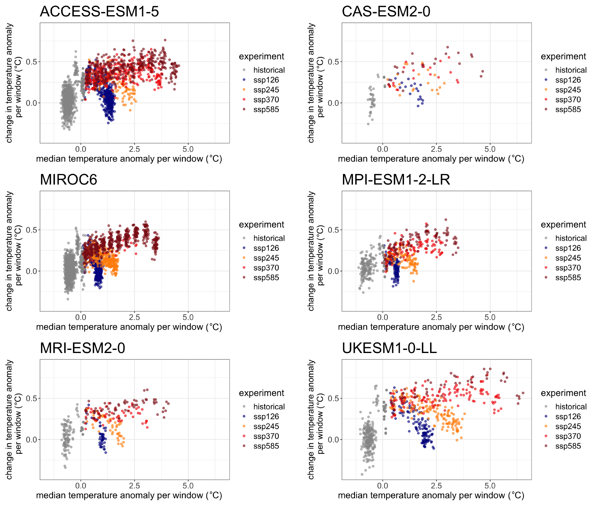
Figure 1 GSAT archive content, plotted in the space of ($T,X\cdot \mathrm{d}T$), i.e., the warming level with respect to the period 1995–2014 (as represented by the median value of the X annual values in the window) and the within-window rate of warming (as represented by a linear trend fitted to the X values) for six of the ESMs used in our emulation exercises. Each point corresponds to a X=9-year-long window in the GSAT time series from an existing scenario simulation, indicated by the color legend.

We now describe the steps of the STITCHES algorithm. See also Fig. A1 for a graphic illustration of it.

1. Time series of annual GSAT from all available simulations of the 21st century by a given model (all scenarios and initial-condition ensemble members) are computed; the time series are made into anomalies with respect to a baseline period of 1995–2014 (we refer to GSAT time series in the following for brevity, but in all cases what we mean is GSAT anomalies time series).

2. An X-year running mean is applied to the GSAT time series, and “pieces” are separated at a regular interval of X years (we use X=9 in our demonstration). We label these pieces derived from the existing ESM simulations as “available”. They identify the potential building blocks for our stitching procedure.

3. For each available piece i of smoothed, annual GSAT we compute its median value, T_i and, as a measure of the rate of temperature change within the piece, the linear trend within the piece, dT_i.

4. The same smoothing and splitting procedure is applied to the trajectory of GSAT for the target scenario to be emulated; we call the result “target pieces”. Note that in the examples of this paper, we derive the target GSAT trajectory from the same ESM, run under a scenario that we choose as the target of the emulation. Therefore, we apply the smoothing procedure to the target GSAT time series as well. Often the real application of the algorithm will target a time series of GSAT that is produced by a simple model, like MAGICC (http://www.magicc.org/, last access: 2 November 2022; Meinshausen et al., 2011) or Hector (Hartin et al., 2015), on the basis of a target scenario. These simple models do not simulate internal variability, and therefore their output is in no need to be smoothed. Also, in these cases the moving average window X may be adjusted by narrowing or extending X until the muted year-to-year variability in the smooth target series produced by the simple model is closely matched.

5. Each target piece and each available piece can now be represented by a point in the two-dimensional space ($T,X\cdot \mathrm{d}T$) (see Fig. 1). In this space, we apply Euclidean distance (d_l2) to determine, for each of the target pieces, its neighbors among the available pieces, within a tolerance Z, used to define a heterogeneous matching neighborhood around each target point of radius $r_i=d_{\mathrm{l}\mathrm{2}}\left(\right(T_i,X\cdot \mathrm{d}{T}_i),\text{nearest\hspace{0.17em} neighbor\hspace{0.17em} })+Z$. The choice of Z could be tailored to the characteristics of each ESM and scenario considered but, importantly, is also directly relevant for the number of matches found and therefore the number of emulated scenarios constructed. Modification of the algorithm could also apply a differential weight to the two dimensions.

6. For each of the target pieces in the sequence spanning the 21st century, one of the neighbors within its Z radius is chosen, and the sequence of chosen available pieces is stitched together sequentially to form the emulated GSAT trajectory. We can randomize the choice of matches or choose nearest neighbors; importantly we do not choose the same piece more than once along the same emulated trajectory (one available piece may be neighbor of more than one target piece along the same target scenario) to avoid unrealistic repetitions, and we do not choose the same piece for the same window in time when constructing more than one ensemble member for the same scenario to avoid what we call “collapsed” ensembles or “envelope collapse”, i.e., trajectories that pass through the same values year after year over a window of time. We apply this restriction both within a single generated trajectory (once an archive window has been used for a target year, it cannot be used again for other target years in that trajectory) and across ensemble members (if two target ensemble members match to the same archive window for the same target year, only one of the ensemble members may keep the match). All these constraints could of course be relaxed.

7. So far the algorithm has produced a new GSAT trajectory, emulating the target one. Importantly, however, the algorithm delivers in essence an ordered series of pointers to the specific experiment–time-window combinations in the archived output from which the chosen neighboring pieces were extracted. Any output from the model (any variable, in isolation or jointly, at any archived frequency and on the native grid of the ESM) can be stitched together according to this sequence, recreating the climate outcome of the desired variable(s) consistent with the emulated scenario.

As pointed out in the description of the algorithm, its parameters (X,Z) are subject to tuning. However, they both have an interpretable function, and only small variations should be acceptable as an alternative setting. In particular,

• X is the size of the smoothing window and the length of the pieces used as building blocks of the synthetic time series. Producing a time series from the available ESM GSAT series whose smoothness matches that of the target series should be the first aim of this parameter, when the target series does not contain internal variability. The use of about 9 years for GSAT has shown in our tests to be a good first guess, but trial and error for the specific simple model used may be in order. When starting from a time series that contains internal variability as our target, the same rule of thumb can be a starting point for the application of the smoothing to both target and available GSAT trajectories. Naturally the time window also dictates the size of the piece: if the window is long enough to erase internal variability, it will prevent any piece from reflecting a single phase of a mode of variability, and therefore, when stitched together, the pieces will not systematically give rise to unrealistic sequences of the phases of those modes. (This may of course fail for the longest multidecadal modes, like North Atlantic Oscillation (NAO) or Pacific Decadal Oscillation (PDO), so if the impact analysis is focusing on the sensitivity of the analyzed system to the phases of these modes, STITCHES may not be the best choice of emulator for this type of impact.)

• Z is the tolerance radius within which we identify neighbors in the two-dimensional space ($T,X\cdot \mathrm{d}T$). The distance along each dimension is immediately interpretable and comparable to the magnitude of the yearly values of GSAT within a piece of the smoothed series (in the T direction) and to the size of its variation within the piece, i.e., a measure of the rate of temperature change within the piece (in the X⋅dT direction) providing guidance in choosing the size of the tolerance. The specific application may allow the tolerance to be increased if a “jump” between pieces is not a concern for the application envisioned, a beneficial choice in enlarging the number of synthetic series that can be constructed from a finite archive of “building blocks”. We also note here that fixing this tolerance in the space of the smoothed GSAT time series leaves open the possibility that the original, i.e., non-smoothed, yearly values can present the occasional large “jump” at the seams where the stitching is performed. This is of course also possible for the additional variables, besides GSAT, that we emulate. Our expectation is that the noise of annual or monthly variability for most variables and spatial scales is large enough to overwhelm the occasional jump at the seam. We show that this is in fact the case in the large majority of cases, so, unless the application is particularly sensitive to year-to-year variations, it might not be considered a fatal defect. Section 3.1.3 presents some results specifically addressing the trade-off between Z and the number of replicates that STITCHES can create. We also note here that in our version of the algorithm we chose a simple Euclidean distance, thus weighing the two dimensions equally, but a user may decide to give larger weight to one of the two.

Table 1 The ESMs, experiments from ScenarioMIP (O'Neill et al., 2016), and ensemble sizes from the PANGEO archive (as of 15 March 2022) used to derive test cases for our emulator.

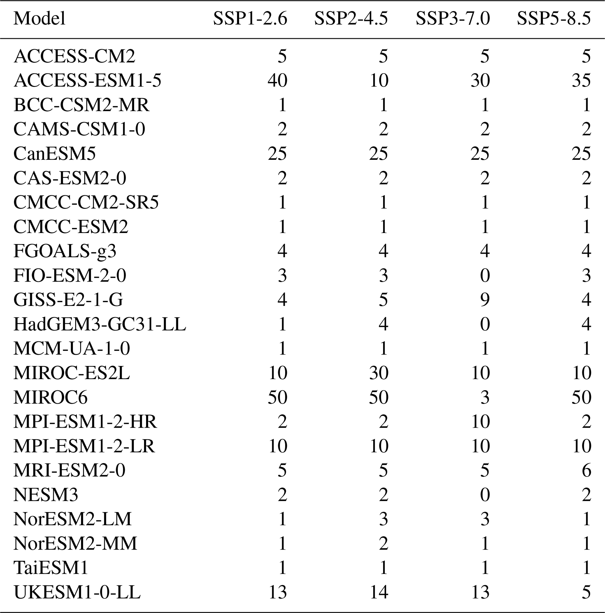
At the time of writing, STITCHES is built to integrate with (and depends on) the PANGEO CMIP6 archive of results (http://gallery.pangeo.io/repos/pangeo-gallery/cmip6/, last access: 15 March 2022). From available runs on PANGEO, we have selected all models, all experiments, and all ensemble members with reported monthly gridded data for surface air temperature and precipitation (we consider a smaller subset that also provides monthly gridded sea level pressure for one particular validation exercise). Model-specific archives are created separately for each ESM. Figure 1 plots the model-specific archive of ($T,X\cdot \mathrm{d}T$) for six ESMs with various size ensembles for each of the scenarios (see Table 1). In the following, we either use a portion of the archive to emulate a left-out portion of the simulations, or we use the whole archive to add new “ensemble members” to some scenarios. The former setup simulates the situation where non-existing scenarios are created from existing ones, but here we also gain the prerogative of validating the emulated scenarios against their true realizations. When the goal instead is to enrich the ensemble size of existing scenarios, one has the option of also using the members of an existing initial-condition ensemble, thus producing trajectories that repeat existing ensemble members' windows, but in a different sequence and mixed with other scenarios' windows. PANGEO contains files where both the historical period and the future have been connected under the label of a specific SSP. Our emulation applies to the entire period (1850–2100), but for brevity in most of the following we label the various cases simply under the corresponding SSP. In fact, most of the ESMs have branched different scenarios from the same historical simulations, so a strict out-of-sample construction of the historical period is in most cases impossible, and the effect is to produce emulated trajectories of the historical period that may use identical pieces to the target from the available. STITCHES' main purpose remains the construction of future scenarios, though, so we do not worry about this detail as we do not predicate our assessment of performance on the historical period.

3 Results

3.1 General tests and validation of the synthetic series

We now show results for several test cases. Table 1 details the models, experiments, and ensemble sizes from the CMIP6 archive available through the PANGEO interface as of 15 March 2022.

3.1.1 Validation of emulated intermediate scenarios

Our first goal is to test the ability of STITCHES to reconstruct ESM-like output for new scenarios using ESM output from existing scenarios. We do so for all available ESMs in the PANGEO CMIP6 archive that provide at least one member under SSP1-2.6 and one member under SSP5-8.5, targeting the two intermediate scenarios SSP2-4.5 and SSP3-7.0 (see Table 1). As already mentioned, when the goal is emulating ESM output for non-existing scenarios, our targets need to be trajectories that reach warming levels within the ones available in the archive, as our algorithm does not allow extrapolation. Similarly, STITCHES cannot emulate overshoot scenarios, given that the archive does not offer a large sample of overshoot experiments from which we can piece out our building blocks (obviously, the cooling behavior of GSAT in an overshoot experiment cannot be sampled from increasing or flat GSAT trajectories.) These considerations could be useful to keep in mind when designing the next phase of ScenarioMIP. Intentionally, we fix the values of the two parameters $(X,Z)=(\mathrm{9},\mathrm{0.075})$, independently of the specific ESM targeted. A specific choice could only ameliorate the performance of our emulator for any given model used as a test case. However, our common choice is the result of considering the behavior of many ESMs and finding values that are consistent with most, so, de facto, these parameters are tailored to some ESMs and less tailored to others. The best performance that we document could be regarded as what is expected when tailoring the parameter values to the specific ESM that we want to emulate.

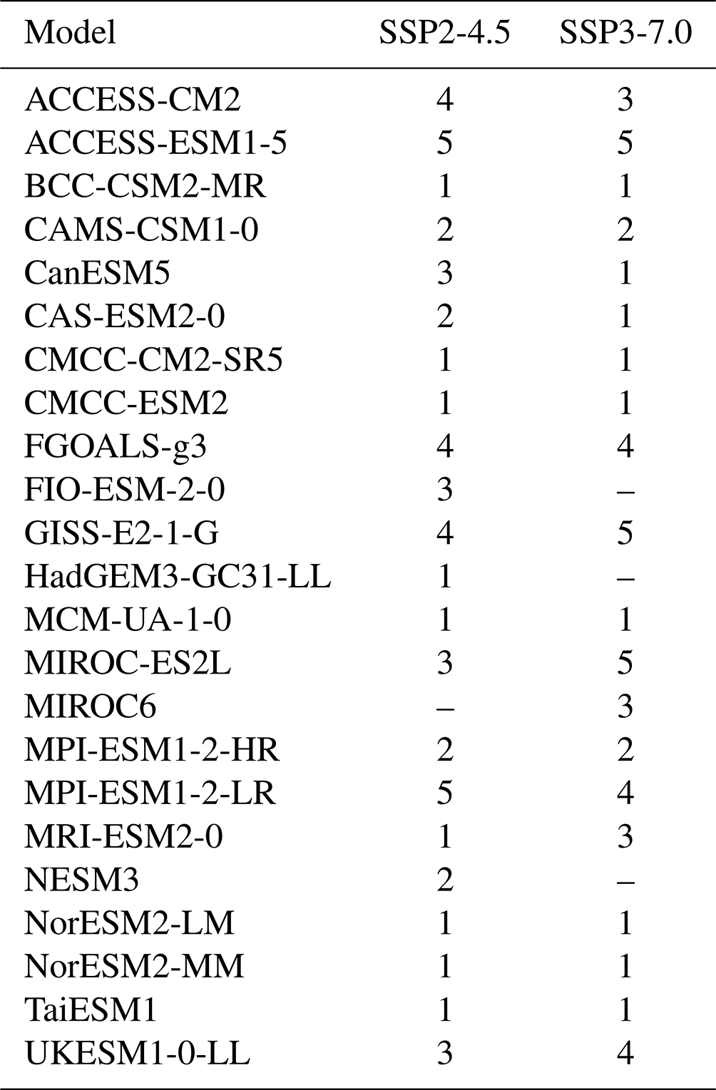
Table 2 lists the number of emulated trajectories for each of the intermediate scenarios targeted and for each of the models. Since this exercise is not about producing many replicates but simply reproducing a target trajectory, for each model we set out to reproduce as many targets' trajectories as there are ensemble members available under SSP2-4.5 or SSP3-7.0 if such a number is less than or equal to five, capping at five the number of targets also for those models with more ensemble members potentially available as targets (see Table 1).

Table 2 The number of emulated trajectories produced to assess the performance of STITCHES in recreating intermediate scenarios (SSP2-4.5 and SSP3-7.0) from the two “bracketing” scenarios (SSP1-2.6 and SSP5-8.5).

As mentioned in Sect. 2 our emulation approach produces the same complex, multidimensional output as an ESM does. Thus, validation could take a practically infinite number of forms over a range of variables in isolation or jointly and over arbitrary spatial scales and timescales. To simplify the task, however, we rely here on the well-known result that – among atmospheric variables that are commonly used for impact modeling – surface air temperature has, relatively speaking, a lower amount of internal variability, and this variability becomes lower the larger the averages taken in the time and space domains. Thus, our validation starts by considering the behavior of annual average GSAT trajectories from STITCHES.

Table 3 For all the models used in our emulation of ESM output under SSP2-4.5 and SSP3-7.0 we report the number of “seams” at which annual GSAT presents a jump that is larger than twice the interannual standard deviation. The latter is computed from either the interannual variations in the archive simulations used in the stitching (in practice, the interannual standard deviations of the stitched trajectories without including the seams in its computation) or the target experiments (the interannual standard deviations of the real series that we are emulating). We also show the total number of seams from which the percentages discussed are computed.

Our first concern is to not systematically introduce significant discontinuities when stitching together separate windows of ESM output, often from altogether different experiments (but always from the same ESM). To this end, we consider the year-to-year difference in the annual GSAT trajectories stitched together. The tolerance allowed for the match (Z=0.075) is responsible for keeping the stitched-together pieces of the smoothed trajectories within a narrow interval of one another but cannot directly control what happens when we recover the stitched-together original trajectories of (non-smoothed) annual values for this validation exercise. These could differ by a larger amount if, by chance, the 9-year pieces happen to end or begin with widely different values. Our concern is that this does not happen systematically. Table 3 reports, for each ESM, how many of these seams (as many for each trajectory as there are 9-year intervals) produce a year-to-year variation that is larger than twice the standard deviation of the real year-to-year variations. The latter are taken as either those from the archive simulations used as building blocks within the stitched trajectories (thus addressing the question “do the seams stand out from the rest of the series within which they appear?”) or those in the target series (thus addressing the question “do the seams stand out compared to the year-to-year variations in the trajectories we want to emulate?”). As can be assessed, this behavior emerges only very sporadically, with most cases well below 10 % of the seams. In fact the mean of these values is just above 5 %, which could be the expected outcome by chance of such an exercise, even if those outliers came from the same distributions used as comparison.

We then compare linear trends fitted to the stitched trajectories to linear trends fitted to the target series by separately fitting a linear trend to the historical period (1850–2014) and the future period (2015–2100). The trends are defined as the angular coefficient of a linear regression of annual mean values of GSAT onto years, and we consider central estimates (by ordinary least squares) and 95 % confidence intervals. We find that in all cases (109 stitched trajectories across the models and the two scenarios) historical trend central estimates for the stitched series fall comfortably within the confidence intervals of the historical trends of the target series. For the future trends, the confidence intervals of the stitched series overlap with the confidence intervals of the trends from the target series in all cases. There are 21 trajectories out of the 109 for which the central estimates fall outside those confidence intervals. In all these cases, the difference between the central estimate and the closest bound of the confidence interval is a very small value: in one single case, the central estimate is outside the confidence intervals by 0.056 ^∘C per decade. In two more cases, the values are between 0.04 and 0.05 ^∘C; six more cases miss by 0.01–0.023 ^∘C per decade, with the remaining 12 cases falling outside the respective confidence intervals only by 0.01 ^∘C per decade or less.

We also compute interannual standard deviations for target and stitched trajectories, finding that once again, historical simulations remain within the ranges of the target trajectories in all cases. For the future period, in 78 % of cases, the stitched series show interannual variability within 20 % of that of the target series. The remaining 24 cases, out of the 109 tested, whose interannual variations fall outside the range of the target series show discrepancies that amount to less than 0.2 ^∘C in all cases, with a median value of 0.004 ^∘C and a third quartile of 0.05 ^∘C. Last, we compute autocorrelation and partial autocorrelation to determine the frequency characteristics of the time series. The results confirm the similarities of stitched and target series; i.e, the emulated trajectories do not show spurious behavior, with discrepancies in the auto-regressive (AR) order estimated only for lags at the margin of statistical significance (not shown).

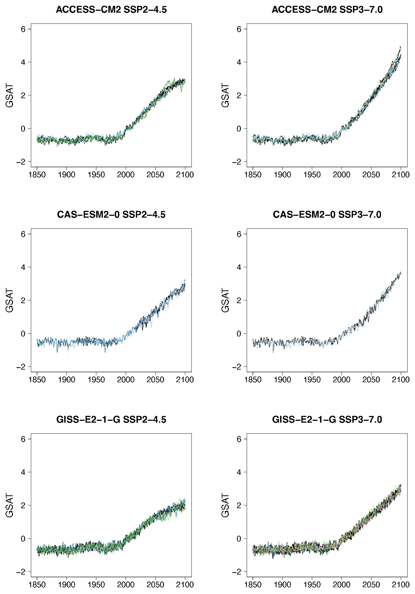
Figure 2 Examples of target (black lines) and stitched (colored) GSAT time series for three ESMs in the PANGEO archive that ran at least one trajectory along the Tier 1 experiments of ScenarioMIP (SSP1-2.6, SSP2-4.5, SSP3-7.0, SSP5-8.5). We choose these three models as they provide differing ensemble sizes (see Table 1) and are characterized by different values of equilibrium climate sensitivity (4.73, 3.40, and 2.72 K, respectively). See Figs. B1–B7 for further examples.

Even if for a large majority of cases the performance of the emulator seems acceptable, and in many cases indistinguishable from the target cases, we underline that some model–experiment combinations appear to be challenging for this uniform setup. Most of these cases coincide with models providing only one ensemble member per scenario, and the spurious behavior is often found at the higher end of the warming range within the scenario emulated, where the only possible matches come from the model's only available SSP5-8.5 trajectory. It is not unlikely that the matches from the higher scenario result in less-than-optimal windows, given the limited choice available for the higher temperature levels. Likely, fixing the tolerance parameter to a tighter value could improve these specific emulation cases or simply fail to create an emulated trajectory so that the user would have an outright warning of the difficulty in matching. Here we remain within a generic setting in order to show the trade-offs at play and identify lessons. We show in Fig. 2 some examples of target (in black) and stitched (colored lines) GSAT trajectories for the two intermediate scenarios and three of the ESMs we test, differing from one another in the size of the archive available and their climate sensitivities (see caption). Additional examples are shown in Figs. B1 through B7 in the Appendix. From these additional figures one can also confirm that the behaviors that appear to deviate from the expected are all at the tail end of the simulations and only for those models that offer only one pair of scenarios in the archive to sample from. This is particularly true when the target scenario is SSP2-4.5, which adds the extra challenge of a trajectory that stabilizes (dT≈0) and needs to find matches among windows that, at those levels of warming, can only come from SSP5-8.5, a scenario of steadily increasing forcing. (As already mentioned, stabilization scenarios together with overshoots pose a challenge to STITCHES given the content of the CMIP6 archive from which we construct our emulations.) In these figures we use a range of colors, from cool to warm hues, to give a sense of the number of trajectories plotted in these spaghetti diagrams: while the target ensemble is always drawn in black lines, the emulated trajectories are in color, with cases showing warmer colors being those where we have created a larger number of stitched trajectories (see also Table 2).

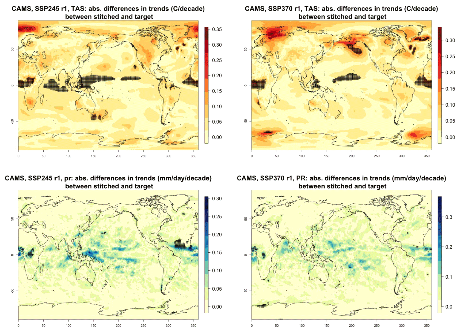
Figure 3 Absolute difference in future trends of monthly temperature variability (TAS) and precipitation (PR) between stitched and target realizations. The value of the difference is expressed by the color scale, and we marked with black crosses those locations where the trends computed from target and stitched time series do not overlap in their 95 % confidence intervals, indicating statistically significant differences. Emulation of CAMS-CM1-0 monthly time series for 2015–2100 under SSP2-4.5 and SSP3-7.0.

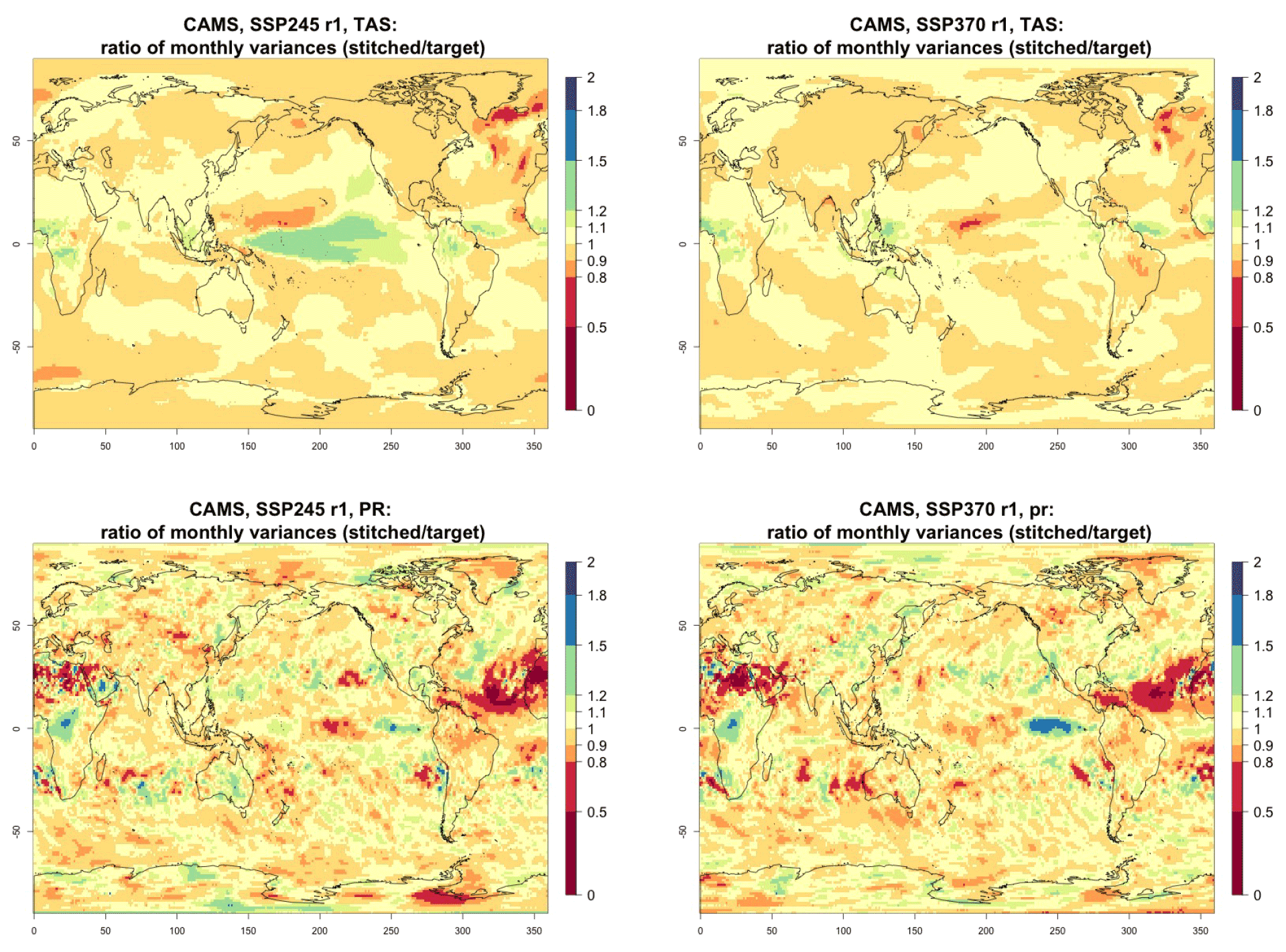
Figure 4 Ratio of monthly variability (standard deviation of residuals from trends) in future temperature (TAS) and precipitation (PR) between stitched (at the numerator) and target (at the denominator) realizations. The value of the ratio is expressed by the color scale, which highlights the transition at 0.8 and 1.2. Emulation of CAMS-CM1-0 monthly time series for 2015–2100 under SSP2-4.5 and SSP3-7.0.

For all cases when the emulation of GSAT time series (made of annual average values) does not present inconsistencies our hypothesis is that noisier quantities would not suffer from detectable discontinuities either. We have tested this expectation for a range of quantities (temperature, precipitation, and sea level pressure) and scales (from subcontinental to local, i.e., grid-point level). Here, as examples, we compare trends and variability (computed as the standard deviations of the residuals from the trend) between stitched and target time series under the two scenarios (over the 2015–2100 period) for temperature (TAS) and precipitation (PR). All metrics here are computed using time series of gridded output at monthly frequency, covering the entire annual cycle, for the length of the emulated output (2015–2100). In the Appendix we show similar results for month-specific output sampling behavior during boreal winter (January) and boreal summer (July), addressing the possibility that the emulation could be differently challenged by stronger or weaker forced trends. We use results from the emulation of two models that represent extremes in the PANGEO dataset, in terms of availability of archive trajectories: CAMS-CM1-0 (with only two ensemble members each for SSP1-2.6 and SSP5-8.5), for which we have derived one emulated trajectory per scenario (SSP2-4.5 and SSP3-7.0), and MIROC6 (with 50 ensemble members for each), for which we have emulated three trajectories per scenario. In the trend figures we blacken grid points where the trends computed from the stitched trajectories are significantly different from those computed from the target trajectory. We use here the same criterion that we applied to the validation of GSAT: trends are significantly different when their 95 % confidence intervals do not overlap. For the analysis of monthly variability we show maps of the ratio of the two variances computed from the stitched and target time series, after removing the linear trends. We consider substantially different variances that are not within 20 % of one another, i.e., whose ratio is either less than 0.8 or more than 1.2. The color bar is chosen to highlight these two thresholds. Figure 3 shows results for the comparison of TAS and PR trends for CAMS-CM1-0, while Figs. C1 through C3 in the Appendix show the corresponding analysis for MIROC6. For temperature, as can be assessed in the top panels of Fig. 3, only isolated patches over the tropical oceans show statistically significant differences in trends. The results for MIROC6, where we can look at three different realizations, show that also for this model's emulation the areas of disagreement consist of isolated patches mostly over ocean regions and not consistent from realization to realization, suggesting the role of internal variability in producing these results rather than a systematic problem with STITCHES. Internal variability is likely responsible for an area in the Arctic showing significant discrepancies in two of the three realizations, but effects of ice-free summer intensified warming (Blackport and Kushner, 2016) or behavior of the Atlantic meridional overturning circulation (AMOC) could also contribute to this limited area of disagreement. For precipitation the inconsistent areas are barely detectable as smaller scatters of points, mostly over the oceans. These results remain essentially unchanged when considering trends for individual months. Figures C4 and C7 show a sample of plots for January and July temperature and precipitation trends for the two models. As can be assessed, the appearance of statistically significant patches of trend disagreement has the same qualitative characteristics as those in the maps showing the comparison of trends computed using the year-long monthly data.

Performance in terms of monthly variability in temperature is within 20 % of the true variability practically over all the land regions and over the large majority of the oceans' areas, with the exception of a systematic bias over the western Pacific cold tongue. Rainfall variability appears less homogeneously accurate, until one realizes that the areas where variability appears inconsistent (i.e., areas where the value of the ratio is smaller than 0.8 or larger than 1.2) coincide with climatologically very dry areas of both the Northern Hemisphere and Southern Hemisphere. In these regions variability is low, and therefore small differences in the numerator and denominator may cause large variation in the ratio, without implying meaningful differences in rainfall behavior.

Last, still concerned with time series behavior, we consider a different quantity altogether: the Southern Oscillation Index (SOI), describing the evolution of the El Niño–Southern Oscillation (ENSO) mode of variability. The SOI is defined as the standardized difference between sea level pressure (SLP) monthly anomalies at Tahiti and Darwin, Australia (https://www.ncdc.noaa.gov/teleconnections/enso/indicators/soi/, last access: 2 November 2022). The negative or positive sign of this difference indicates abnormally warm or cold ocean waters across the eastern tropical Pacific, associated with El Niño or La Niña episodes. The index, despite being a uni-dimensional time series, reflects the behavior of a coherent spatial field (SLP) at monthly frequency. Its frequency characteristics are important to preserve, as the opposite phases of the SOI have been found to be associated with significant shifts in the weather of regions having strong teleconnections, causing droughts or intense precipitation and cooler- or warmer-than-average conditions (Mason and Goddard, 2001; Lenssen et al., 2020). Therefore, for impact analysis, we would not want to produce time series of this index with a spurious behavior, compared to the corresponding continuous output of the emulated ESM. Thus, we perform a comparison of the characteristics of the true and emulated SOI time series using (partial) auto-correlation function and spectral density estimates. Note however that we are not comparing these frequency characteristics to observations, which is not the point of our validation exercise. We consider this validation particularly important, both because of the salience of ENSO behavior for many types of impact and because the frequency characteristics of this mode of variability are close to our 9-year windows.

Figure 5 presents target and stitched time series of the ENSO index for one of the models (CAMS-CM1-0) and three 20-year windows along the two scenarios emulated. As can be gauged, the three pairs of time series appear similar in magnitude and oscillatory behavior. In order to confirm the latter, we show in Fig. 6 the (partial) auto-correlation functions of the corresponding time series. This analysis produces indistinguishable lag patterns and, importantly, does not reveal any spurious behavior at 9-year lags. Figures D1 through D6 in the Appendix confirm that results are similar for three emulated ensemble members under each scenario for MIROC6. Further, we show in Fig. D7 the spectral densities of the entire time series, comparing target and stitched and showing how the densities of the stitched trajectories have a behavior that is qualitatively and quantitatively (up to what appears as some noisy behavior at very low frequencies) consistent with that of the target trajectories.

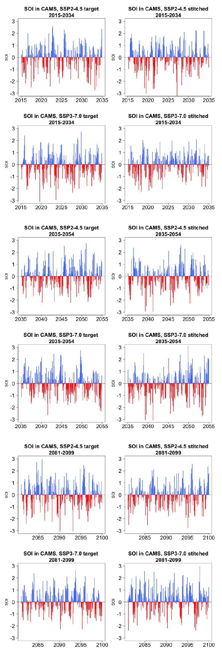
Figure 5 Examples of target (left) and stitched (right) SOI time series for three 20-year windows along the length of the simulation: 2015–2034 in the top four panels, 2035–2054 in the middle four panels, 2081–2100 in the bottom four panels. Results from emulation of SSP2-4.5 and SSP3-7.0 for CAMS-CM1-0.

Figure 6 Auto-correlation functions (ACFs) and partial auto-correlation functions (PACFs) for real and stitched SOI time series. Top two rows: SSP2-4.5 ACF for target and stitched series and respective PACFs. Bottom two rows: SSP3-7.0 ACF for target and stitched series and respective PACFs. (Our software – R function acf(..,type="partial") – does not define the PACF at lag zero.)

On the basis of these results we confirm the correctness of our expectation that, after validating the statistical characteristics of a large-scale, low-frequency quantity like annual GSAT, further validation of emulated variables at grid-point scale and higher temporal frequency do not seem to present larger challenges. The higher noise of these quantities indeed accommodates the discontinuities introduced by their emulation.

3.1.2 Validation of emulated initial-condition members

Our emulator can also be used to provide multiple ensemble members under the same scenario, akin to initial-condition ensembles. For this type of application, besides the necessary validation of the individual members according to the above-described metrics, we want to validate the properties of the synthetic ensembles as such, comparing their mean behavior and their spread to those of real initial-condition ensembles from the same ESM. Figures E1 through E5 show the resulting ensembles for a number of experiments that we conducted over several ESMs and the two scenarios SSP2-4.5 and SSP3-7.0. We chose models that provided at least five 21st-century trajectories of the Tier 1 scenarios. As mentioned in Sect. 2, this exercise is conducted by using the entire archive available, as we mimic a situation where we are not creating a new scenario but augmenting the size of an initial-condition ensemble run under existing ones.

We adopt the two-dimensional metric of performance introduced by Tebaldi et al. (2020). We indicate with y a quantity derived from the true ensemble and with $\widehat{\mathit{y}}$ the same quantity derived from the emulated ensemble. Further, we indicate with angle brackets the ensemble-average operation. The two-dimensional metric is then defined as

$$\begin{array}{}\text{(1)}& E_r(\mathit{y},\widehat{\mathit{y}})=\left({\displaystyle \frac{|\langle \mathit{y}\rangle -\langle \widehat{\mathit{y}}\rangle |}{\sqrt{\langle (\mathit{y}-\langle \mathit{y}\rangle {)}^{\mathrm{2}}\rangle }}},\sqrt{{\displaystyle \frac{\langle (\widehat{\mathit{y}}-\langle \widehat{\mathit{y}}\rangle {)}^{\mathrm{2}}\rangle }{\langle (\mathit{y}-\langle \mathit{y}\rangle {)}^{\mathrm{2}}\rangle }}}\right).\end{array}$$

Table 4 The two components of the E_r metric, E₁ and E₂, computed for several experiments across ESMs, scenarios, and number of available archive trajectories from which to create the stitched ensembles. Numbers in columns 4 through 9 represent fractions of the target ensemble standard deviation (see Eq. 1).

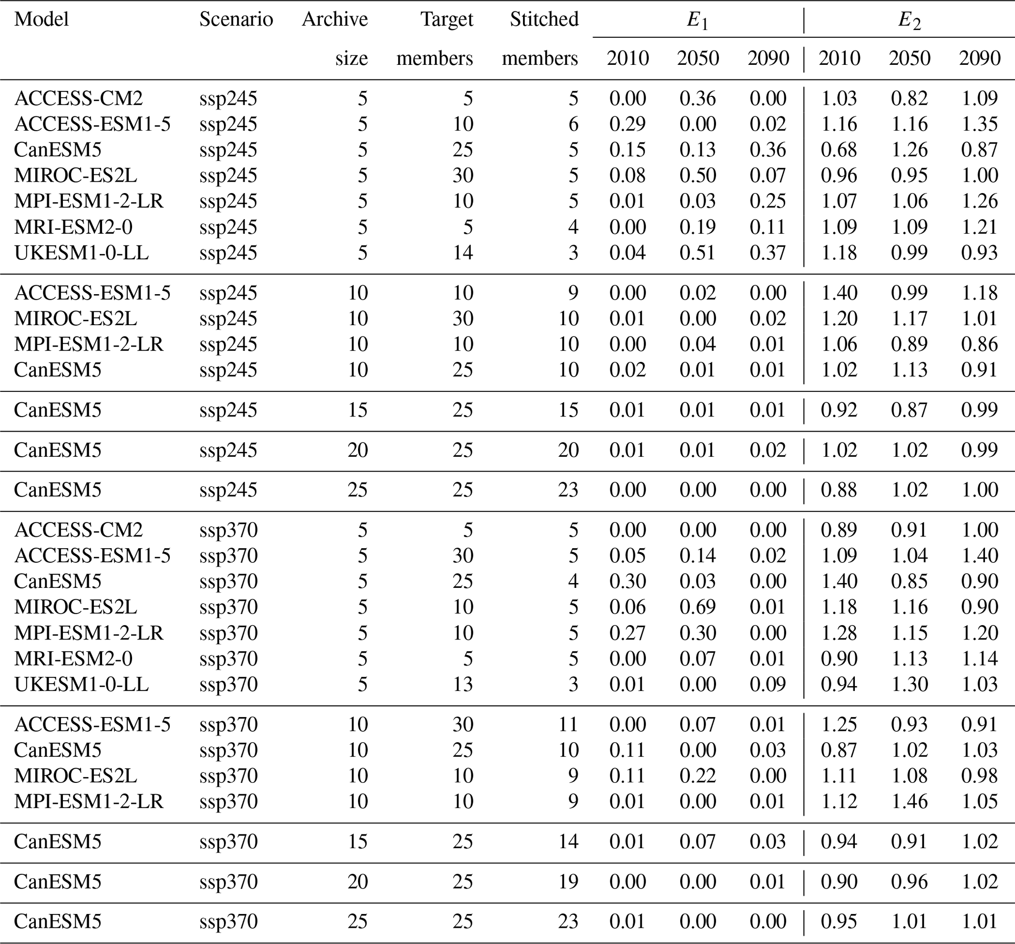
Its first component (which we indicate below as E₁) measures the systematic bias between the means of the true and the synthetic ensembles, normalized by the true ensemble standard deviation. The second, E₂, is defined as the ratio between the synthetic and the true ensemble standard deviations. In a perfect emulation, $E_r=(\mathrm{0},\mathrm{1})$. It is useful to note that the magnitude of these metric components is expressed as a fraction (or multiple) of the true ensemble standard deviation, allowing a judgment of the size of the discrepancies introduced by STITCHES as they compare to the true internal variability in the target ensemble. Here as before we focus on annual series of global mean temperature. Table 4 reports the values of E₁ and E₂. The number under the column labeled “Archive size” indicates how many 21st-century trajectories were available for each of the four scenarios in the archive to create 9-year building blocks for STITCHES. Note that when a model provided numerous trajectories to build from, we tested the performance for increasing sizes of the archive (e.g., for the CanESM5 model we repeat the exercise using 5-, 10-, 15-, 20-, and 25-member initial-condition ensembles for each scenario). The following two columns in the tables list the size of the target ensemble emulated, which is therefore available for validation (y), under “Target members”, and the size of the stitched ensemble, under “Stitched members”, which is the number of additional trajectories created by STITCHES that could be added to the existing ensemble. We choose 3 years along the 21st century, 2010, 2050, and 2090, and we utilize 9-year windows around those years to compute Eq. (1) (similar results were obtained by using a shorter 5-year window).

Several outcomes can be gleaned from Table 4. STITCHES' trajectories have mean and variability characteristics within a small window of the target ensembles in the great majority of cases. Of course the application should dictate the standard that needs to be met by the synthetic ensembles, but if discrepancies of up to 25 % or 30 % of the true internal variability are acceptable, most cases described in the table would meet that standard, and in the great majority of cases by a large margin, especially once the ensembles available from which we sample building blocks have at least 10 members. This exercise uses a tolerance value Z=0.075 across the board, but tuning the value to specific ESM characteristics could ameliorate some of the worse performances. A look at the best performances suggests what we should expect if the tuning were conducted specifically to each ESM's characteristics of variability. Section 3.1.3 below further expands on the relation between the tuning parameter Z, the size of the ensembles that STITCHES can create, and the values of the E_r metric.

We have performed the same exercise by limiting the archive to the two bracketing scenarios, SSP1-2.6 and SSP5-8.5, and trying to construct ensembles for SSP2-4.5 and SSP3-7.0. In this case STITCHES is significantly challenged: its performance, as measured by the E_r metric, is significantly diminished and, when comparing what happens for the same model and increasing numbers of archive members, unpredictable, due to the fact that the algorithm randomizes both the identity of the archive members and the choice of the nearest neighbors to construct the emulated output. Table F1 reports these discrepancies. A look at Fig. 1 may suggest the nature of the challenge here, because of the relatively extreme nature of SSP5-8.5 values compared to SSP2-4.5 in particular. Section 3.1.3 below also discusses this aspect. We argue that this challenge could be lessened by a more deliberate design of ESM experiments in relation to the ($T,X\cdot \mathrm{d}T$) space. Additionally, as has been argued recently, SSP5-8.5 may represent an obsolete or at least improbable scenario (Hausfather and Peters, 2020), and therefore the range to be explored by future scenarios could be narrower in the next phase of CMIP experiments.

3.1.3 Trade-offs between generated ensemble size and Z

The size of a stitched ensemble targeting a given experiment is directly related to the number of ESM ensemble members present in the archive, as well as the tolerance for matching, Z. Larger values of Z result in larger numbers of stitched ensemble members, until the archive is exhausted. It is unlikely that a closed-form relationship between archive size (Z) and size of the stitched ensemble exists, as another factor in the success of the emulation is how similar the GSAT trajectories in the archive are to the target and archive scenarios, not only in median value but also in rate of warming, the two dimensions of our neighborhood. Instead, we present empirical estimates, for each ESM separately, of a conservative cutoff value for Z, Z_cutoff, that should safely result in generated ensemble members satisfying our validation criteria presented in the above Sects. 3.1.1 and 3.1.2. Specifically, we identify the Z_cutoff at which the generated ensemble size appears to saturate while still maintaining small E_r values. Thus, using Z values beyond the provided Z_cutoff provides no additional benefit.

To identify Z_cutoff for each experiment of each ESM, we conduct a sweep of Z values ranging from 0.04 to 0.3 ^∘C. As noted in step 6 of the algorithm, the actual matches within each Z neighborhood are drawn randomly for stitching a trajectory. Therefore, at each Z value tested, we perform 50 of these random draws of the STITCHES algorithm for generating the largest possible collapse-free ensemble, targeting both experiment SSP2-4.5 and SSP3-7.0, and using the full archive for that ESM (see Table 1). We calculate the same E_r statistics above for both GSAT and the GSAT differences “at the seams” computed over the annual time series of stitched GSAT for each draw of a full generated ensemble. Z_cutoff is identified as the largest tolerance value that keeps the average value across draws of the two pairs of these metrics for each target ensemble below 10 %. Generally, it is the E₂ dimension of the GSAT differences at the seams when targeting SSP2-4.5 that is largest of the four error metrics across both target experiments; i.e., the standard deviation of the generated interannual jumps differs from the standard deviation of the interannual jumps of the target. This exercise should be repeated for other values of X (number of years in a window), particularly for values substantially further away from the X=9 value considered in this work. The metarepository for this paper (see “Code and data availability”) includes the experiment scripts used for this exploration, which users may adapt.

Z_cutoff values and the corresponding draw-averaged generated ensemble size for each experiment–ESM combination are reported in Table 5. Increasing the tolerance beyond these Z_cutoff values can increase the generated ensemble size, but with larger errors, meaning potentially the stitched realizations at that point may not behave well. For example, at Z_cutoff=0.25, ACCESS-CM2 can stitch seven realizations targeting SSP2-4.5 but at a max error of 11.6 % (E₂ of the GSAT differences in this case). Values of E₂ of the GSAT differences this large may correspond to stitched GSAT trajectories that clearly feature abrupt switching between windows of distinctly SSP1-2.6 and SSP5-8.5 behavior rather than actually emulating an SSP2-4.5 trajectory. Finally, if one wishes to select a single tolerance to use for emulation of both SSP2-4.5 and SSP3-7.0 (and likely for similar, novel, intermediate scenarios), the larger Z_cutoff should be used. For example, if one wished for a single Z_cutoff value for CanESM5, Z_cutoff=0.13 would provide generated ensemble sizes of 25 each for both SSP2-4.5 and SSP3-7.0 (with a draw-averaged max E_r of 5.1 % rather than 4.3 %).

Table 5 For each ESM and the two scenarios targeted by the emulation, we show the size of the archive, the number of trajectories used as target, and the number of stitched trajectories obtained from them for the value of Z_cutoff, which keeps the metric E_r, when averaged across 50 draws, at the maximum value indicated along the column E_r^∗. Thus, by $E_r^{\ast }$ we indicate the result of averaging E₁ and E₂ (see Eq. 1) separately over the 50 draws and taking the maximum of the two average values. We refer to Sect. 3.1.3 for details.

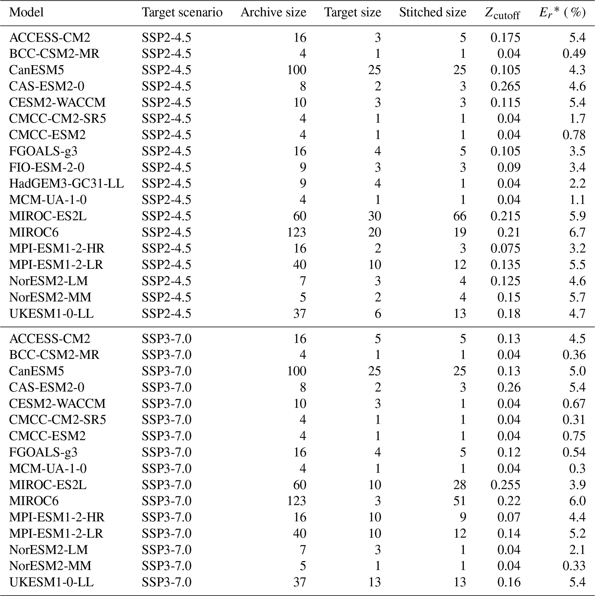
By comparing the generated ensemble size from Table 5 with the CMIP6 archive sizes outlined in Table 1, we see that for most ESMs, STITCHES can generate a stitched ensemble of the same size as the target ensemble. The cases with large archive sizes (CanESM5, MIROC-ES2L, MIROC6, and MPI-ESM1-LR), however, make it clear that the size of the stitched ensemble is not necessarily a direct function of the availability of runs in the archive or the size of the target ensemble but depends on the proximity in ($T,\mathrm{d}T\cdot X$) space of the target windows to the archive windows. A look at the panels in Fig. 1 gives a good representation of the challenges, as SSP370 appears to lie comfortably within the envelope of the SSP585 runs, whereas SSP126 and SSP245 appear more isolated. We discuss the implications of this in Sect. 4. The Z_cutoff values in Table 5 are also not the final limits on where good matches may be generated. Specifically, because we start the matching neighborhood for each target point by finding the nearest neighbor in the archive first and then adding the tolerance to that distance (step 5 of the algorithm), there is a heterogeneity of matching neighborhood size for each target point even within a single trajectory. A different choice could uncover further results; however the choice to begin with nearest neighbors was made for convenience: at Z=0, the stitched trajectory returned is simply made up of the nearest neighbor points in the archive. Finally, there is utility in the stochastic draws used in this exercise as well. Multiple draws of generated ensembles fed through impact models may lead to new insights, despite the fact that appending multiple draws together into a single “super”-generated ensemble is not advised as it will bypass the restriction on generated ensemble envelope collapse enforced in step 6 of our constructive algorithm.

4 Discussion and conclusions

We have proposed an algorithm, STITCHES, that exploits available simulations of future scenarios to deliver fully consistent and complete ESM-like output according to a new scenario, based on the trajectory of global temperature that the new scenario produces. STITCHES works by stitching together decade-long windows (we use 9 years to be precise, but the length of the window is a tunable parameter) of existing 21st-century ESM simulation output. These windows are chosen on the basis of their corresponding GSAT absolute value and derivative, identified to match those of subsequent windows of the GSAT time series derived from the scenario to be emulated. The same algorithm can also be used to enrich the size of existing initial-condition ensembles. We have demonstrated the algorithm performance using the PANGEO CMIP6/ScenarioMIP archive of the four Tier 1 experiments, SSP1-2.6, SSP2-4.5, SSP3-7.0, and SSP5-8.5, targeting the emulation of the two intermediate scenarios.

Our numerous validation tests have shown that the stitched time series do not reveal in the great majority of cases spurious behavior, even when the matching criteria are set without being specifically tailored to the internal variability in the ESM to be emulated. We have shown that jumps or discontinuities are seldom created at the global scale, when considering surface temperature. Since surface temperature is the smoothest quantity among the variables commonly used to drive impact models, our hypothesis has been that any other variable at the global or regional scale, and for yearly frequencies or higher, would be even better behaved at the seams, since the larger internal variability would even more easily overwhelm discontinuities introduced by STITCHES. We have confirmed this hypothesis with case studies for gridded temperature and precipitation at the monthly frequency. We have also shown that for ENSO, a salient mode of variability for many natural and human systems, a 9-year window does not introduce odd frequency artifacts in the SOI time series. This should reassure modelers of impacts sensitive to ENSO teleconnections. Synthetic “large ensembles” created to enrich initial-condition experiments show an ensemble behavior within a small neighborhood of the truth (in most cases much narrower than ± 25 %–30 % of the target ensemble variability) in terms of ensemble mean and ensemble variance.

Our exploration of the performance of the algorithm as a function of the available archive size suggests that five 21st-century trajectories ensure an acceptable performance (according to our metrics), and even smaller archive sizes often – if not always – deliver acceptable stitched new trajectories. Thus, for modeling centers choosing to invest resources in future scenario simulations, running a well-chosen small set of trajectories that span what the community considers the plausible range of GSAT absolute change and rates of change, or radiative forcing, could suffice, and the center could be better served by focusing on running a few initial-condition ensemble members for each trajectory rather than investing in multiple similarly shaped scenarios. This also entails savings for the community that provides the direct forcing inputs to ESMs by translating IAM output into spatially and temporally resolved forcing fields for scenario simulations. Resources in post-processing of model output, extending to the need of downscaling and bias correcting, will be saved as well, as the emulated scenarios can be built from those post-processed ones.

Of course, our proposal does come with caveats. ENSO frequencies are right around the timescale that is preserved by 9-year windows, but there exist slower modes of variability in the climate system whose single phases may instead align with such a time span and whose coherent behavior would be broken by our window splitting and stitching together. Thus, any investigation of impacts that are known to be sensitive to low-frequency variability at decadal timescales needs to proceed with caution, try lengthening the window X, or not use STITCHES' output at all. Similarly, any impact that depends on quantities whose integral is important rather than their instantaneous value cannot use the output from STITCHES if such integral frequently, or by definition, extends over the window size. Pre-eminently, sea level rise derived from ocean heat content, which is a path-dependent quantity, cannot use the ocean heat content that comes with a STITCHES scenario, which would not be coherent with the scenario path. Similarly, mega-droughts lasting over a decade cannot be coherently represented in a scenario emulated by STITCHES.

There are more subtle aspects of stitched scenarios that may pose questions of fidelity and representativeness. We have not addressed the challenges that short but intense forcing episodes, like volcanic eruptions, may pose, since we have focused the application of STITCHES on future scenarios, which do not represent them. A careful look at Fig. 1 can highlight a region of the space populated by gray dots (the historical part of the simulations) showing a peculiar pairing of absolute temperature anomalies and rate of change in the region around $T=-\mathrm{0.01}$ compared to that around T=0.01. This would suggest a specific behavior of GSAT while recovering from volcanic eruptions that is not easily emulated by finding analogs in the historical period (away from volcanic episodes). One other possible challenge to STITCHES has to do with regional and/or short-lived forcers like land use and aerosols, which usually vary across scenarios. STITCHES would not closely represent these forcers if the scenario to be emulated contained different regional patterns or histories for them compared to the scenarios used to generate the pieces. Thus, if those regional, short-lived forcers create climate signals that significantly alter the nature of the output they appear in, STITCHES would not replicate those signals. This is, however, not different from what happened in any analysis using time sampling (King et al., 2018) or simple pattern scaling. Thus, here we work under the assumption that – amidst the uncertainties in different ESM responses and impact modeling affecting regional climate and impact outcomes – the signals introduced by regional and/or short-lived forcers would not be consequential to the results. We do encourage deeper exploration of these questions.

Last, some technical aspects of our algorithm will benefit from further analysis and considerations: possibly some applications may be able to relax the tolerance parameter and thus set the conditions for easier matching and more numerous stitched realizations. This might be true of applications that would not be too sensitive to interannual differences. In contrast, tightening the tolerance to match specific ESMs' internal variability will be beneficial in eliminating spurious behavior that we have documented in some cases, especially when the archive of available runs is poor. More generally we could choose a different distance measure in the ($T,X\cdot \mathrm{d}T$) space or a completely different space over which to look for nearest neighbors, but the necessity of conforming to what a simple model can produce on the basis of a new emission scenario needs to be kept as a consideration.

We would have liked to make more than just a rule-of-thumb recommendation for the number of ensemble members that modeling centers should run and link that formally to the number of expected trajectories created by STITCHES. That said, the last phases of CMIP have shown that, ultimately, modeling centers will commit what they can to running future scenarios. Our proposal shifts those energies and resources away from running a number of scenarios of similar shapes. One additional possibility that we have not explored is utilizing idealized experiments like 1 % CO₂ among the building blocks, consistently with our discussion of the secondary relevance (until proven wrong) of forcing agents other than well-mixed greenhouse gases.

In addition to stabilized scenarios, which were not systematically explored by the last set of simulations and that therefore would pose a challenge to STITCHES, STITCHES cannot emulate at this time another type of scenario that is becoming more and more prominent in the policy discourse: the overshoot, i.e., a scenario that presents a peak and decline in forcing and therefore global average temperature. If a range of overshoots are sought, there is the need to run with ESMs some cases with different steepness and length in order to provide building blocks of decreasing temperature at different rates.

Despite the warranted caveats, we believe that our proposal has desirable outcomes for the research communities occupied with climate, scenario, and impact modeling. Impact and IAM modelers that want to assess impacts for scenarios other than those that have been generated by ESMs, including endogenously generated forcing pathways within IAMs, could rely on STITCHES to fill the gaps, acquiring the same type of output, in all its complexity and refinement, that an ESM would provide. An “online” application of STITCHES within an IAM simulation could allow climate impacts to be modeled within the evolving system that the IAM is modeling and therefore represent fully consistent feedback loops between climate change drivers (emissions) and climate change impacts. The wider impact research community could choose from a larger set of trajectories and possibly a larger set of initial-condition ensembles than the ESM ran. Climate modelers can reduce the effort devoted to preparing inputs for, setting up, running, and post-processing future scenarios. We acknowledge here the richness of climate model output archives already at our disposal (CMIP5, CMIP6, SMILES), which right now provide a wide variety of building blocks. The next phases of CMIP could complement what is available now by deliberately exploring types of scenarios that are not well represented in the current archives, like stabilized trajectories and overshoots. The challenge would lie in choosing the best set of runs to optimally populate the ($T,X\cdot \mathrm{d}T$) space to maximize the number and shape of attainable new trajectories from the existing ones. The deployment of STITCHES, in concert with other emulators like MESMER-M and MESMER-X (Nath et al., 2022; Quilcaille et al., 2022) and PREMU (Liu et al., 2022), which are intended to produce new realizations of internal variability, could then complement and enrich the effort of the ESM community.

Appendix A: A diagram of the STITCHES algorithm

Figure A1 Numbers to the side of the boxes refer to the algorithm steps detailed in Sect. 2.

Appendix B: Additional GSAT time series for intermediate scenarios

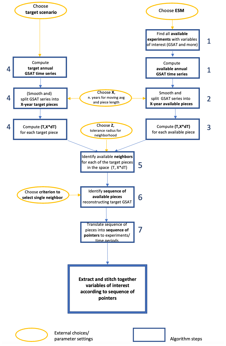
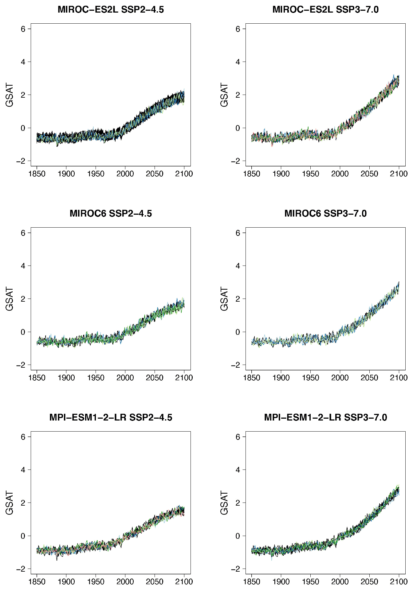
Figure B1 Examples of target (black lines) and stitched (colored) GSAT time series for ESMs in the PANGEO archive that ran at least one trajectory along the Tier 1 experiments of ScenarioMIP (SSP1-2.6, SSP2-4.5, SSP3-7.0, SSP5-8.5). We use the two bracketing scenarios and emulate trajectories that follow the two intermediate scenarios.

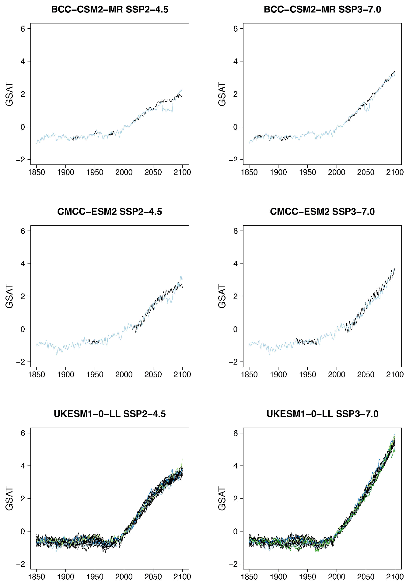
Figure B2 Examples of target (black lines) and stitched (colored) GSAT time series for ESMs in the PANGEO archive that ran at least one trajectory along the Tier 1 experiments of ScenarioMIP (SSP1-2.6, SSP2-4.5, SSP3-7.0, SSP5-8.5). We use the two bracketing scenarios and emulate trajectories that follow the two intermediate scenarios.

Figure B3 Examples of target (black lines) and stitched (colored) GSAT time series for ESMs in the PANGEO archive that ran at least one trajectory along the Tier 1 experiments of ScenarioMIP (SSP1-2.6, SSP2-4.5, SSP3-7.0, SSP5-8.5). We use the two bracketing scenarios and emulate trajectories that follow the two intermediate scenarios.

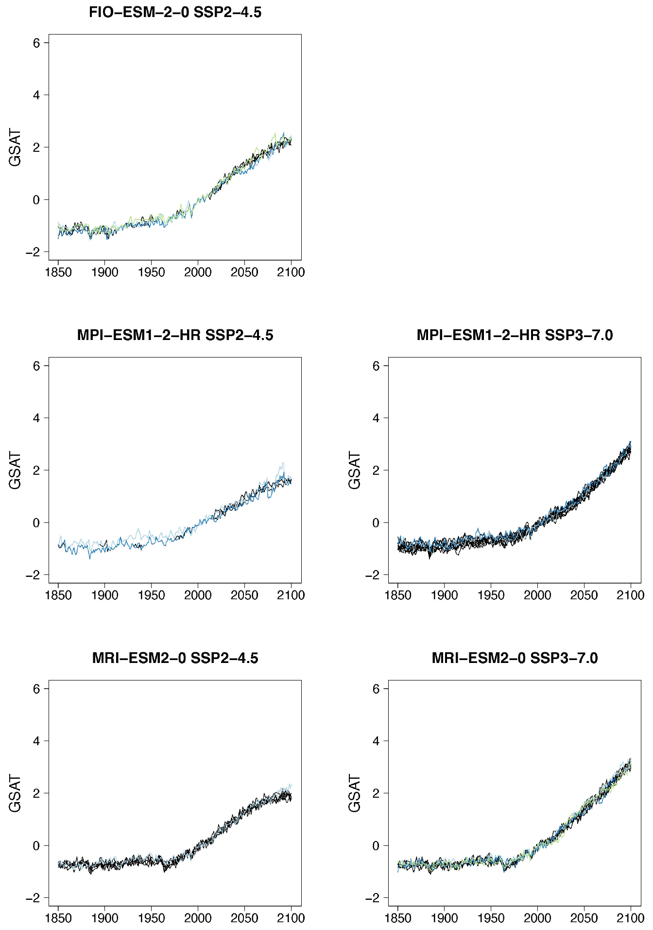
Figure B4 Examples of target (black lines) and stitched (colored) GSAT time series for ESMs in the PANGEO archive that ran at least one trajectory along the Tier 1 experiments of ScenarioMIP (SSP1-2.6, SSP2-4.5, SSP3-7.0, SSP5-8.5). We use the two bracketing scenarios and emulate trajectories that follow the two intermediate scenarios.

Figure B5 Examples of target (black lines) and stitched (colored) GSAT time series for ESMs in the PANGEO archive that ran at least one trajectory along the Tier 1 experiments of ScenarioMIP (SSP1-2.6, SSP2-4.5, SSP3-7.0, SSP5-8.5). We use the two bracketing scenarios and emulate trajectories that follow the two intermediate scenarios.

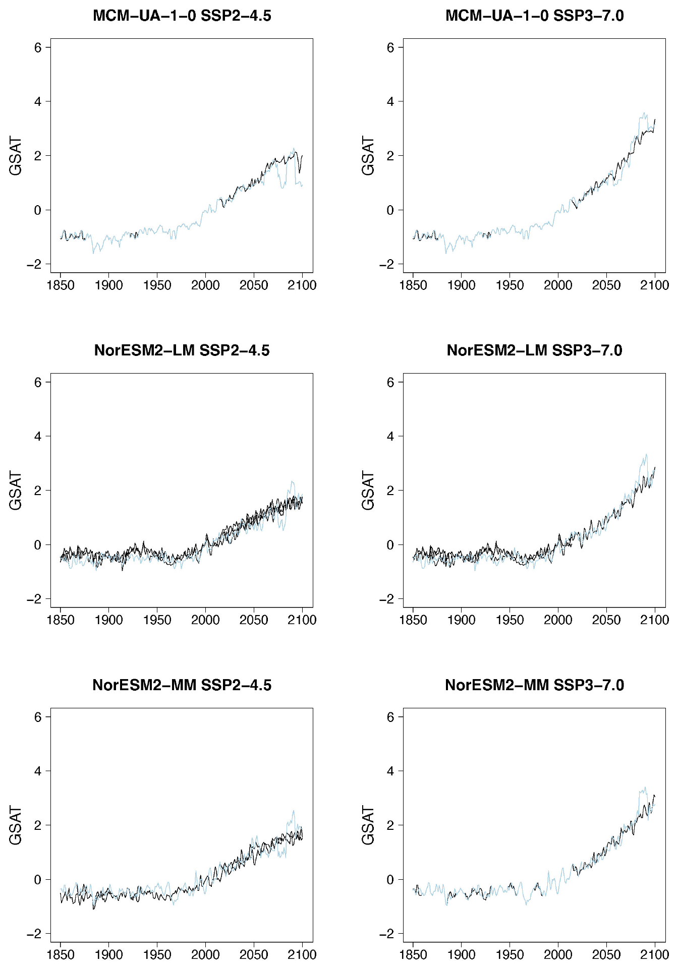
Figure B6 Examples of target (black lines) and stitched (colored) GSAT time series for ESMs in the PANGEO archive that ran at least one trajectory along the Tier 1 experiments of ScenarioMIP (SSP1-2.6, SSP2-4.5, SSP3-7.0, SSP5-8.5). We use the two bracketing scenarios and emulate trajectories that follow the two intermediate scenarios.

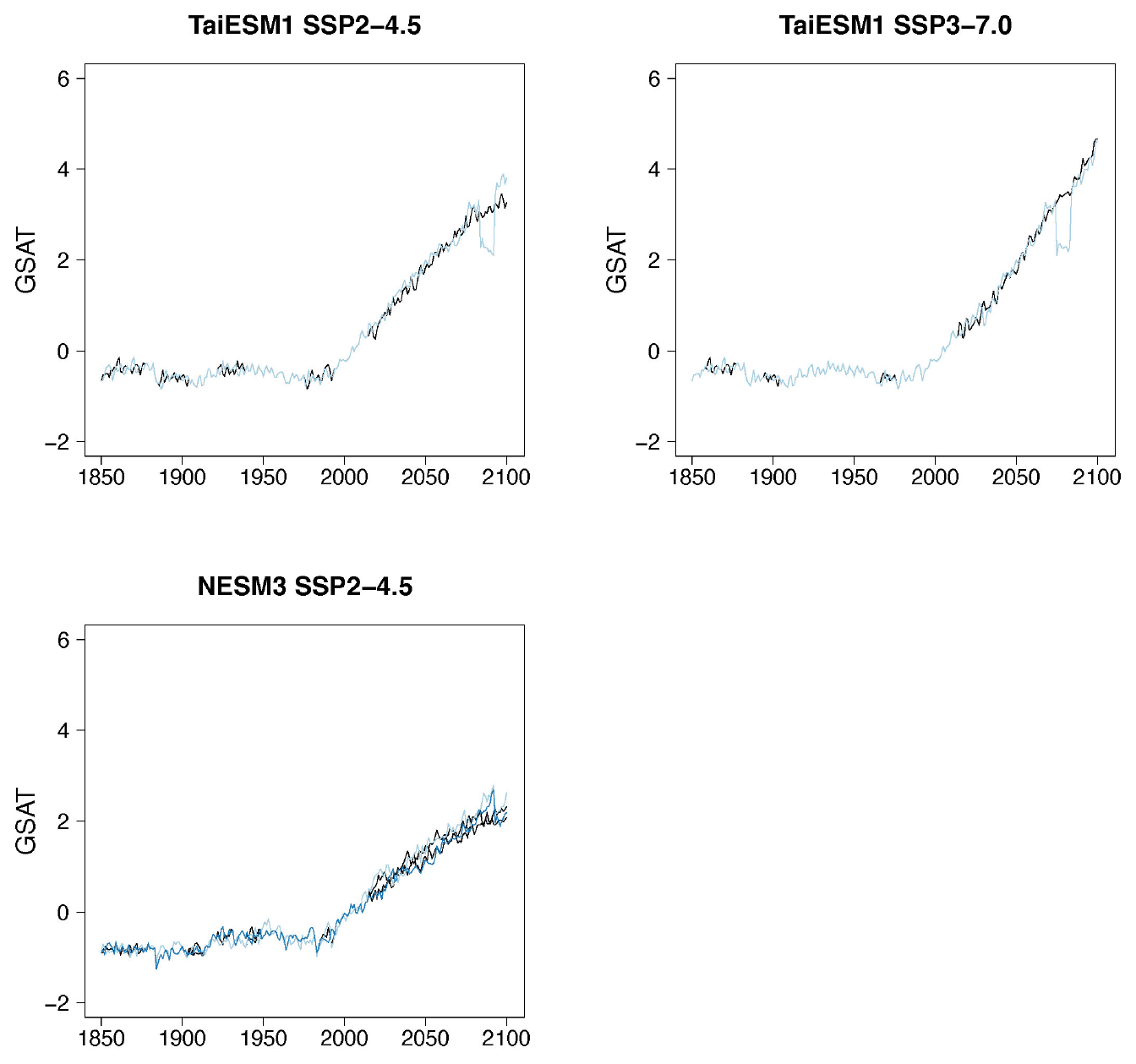
Figure B7 Examples of target (black lines) and stitched (colored) GSAT time series for ESMs in the PANGEO archive that ran at least one trajectory along the Tier 1 experiments of ScenarioMIP (SSP1-2.6, SSP2-4.5, SSP3-7.0, SSP5-8.5). We use the two bracketing scenarios and emulate trajectories that follow the two intermediate scenarios.

Appendix C: Additional trend and variability analysis of gridded data

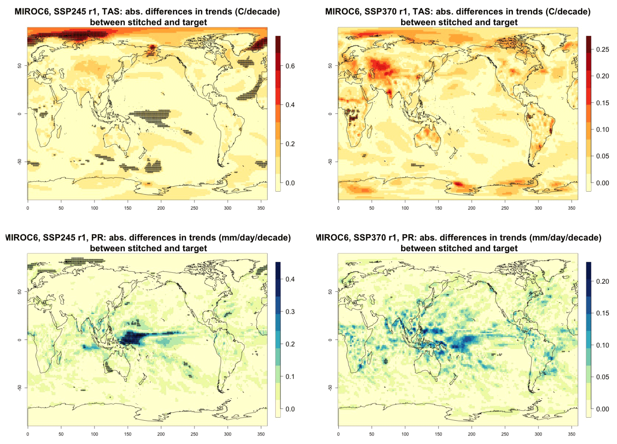
Figure C1 Absolute difference in decadal trends of temperature (TAS) and precipitation (PR) between stitched and target realizations. The value of the difference is expressed by the color scale, and we marked as significant with black crosses those locations where the 95 % confidence intervals of the trends computed from target and stitched time series do not overlap, indicating statistically significant differences. Emulation of MIROC6, monthly time series over 2015–2100, for SSP2-4.5 and SSP3-7.0. First realization.

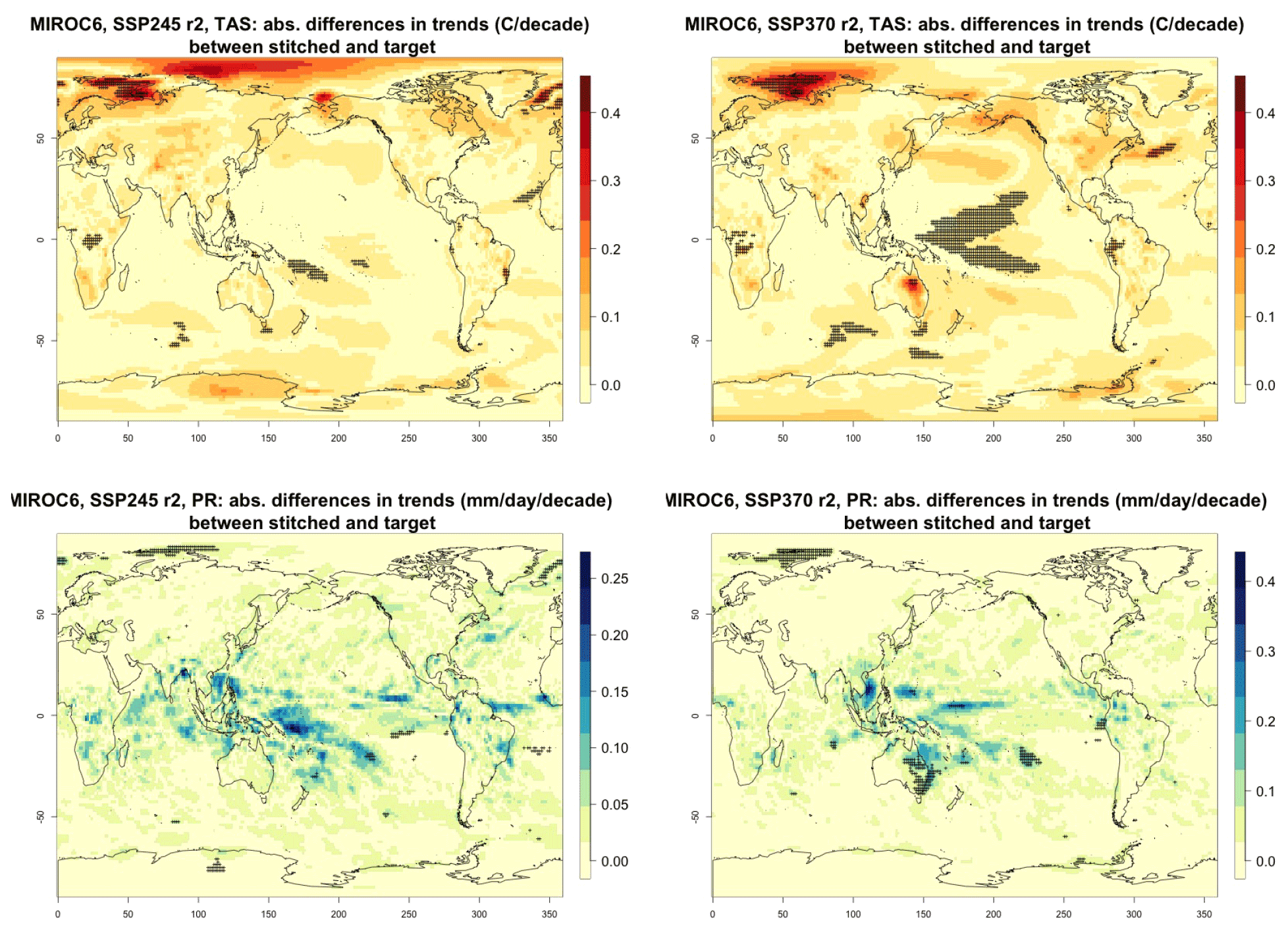
Figure C2 Absolute difference in decadal trends of temperature (TAS) and precipitation (PR) between stitched and target realizations. The value of the difference is expressed by the color scale, and we marked as significant with black crosses those locations where the 95 % confidence intervals of the trends computed from target and stitched time series do not overlap, indicating statistically significant differences. Emulation of MIROC6, monthly time series over 2015–2100, for SSP2-4.5 and SSP3-7.0. Second realization.

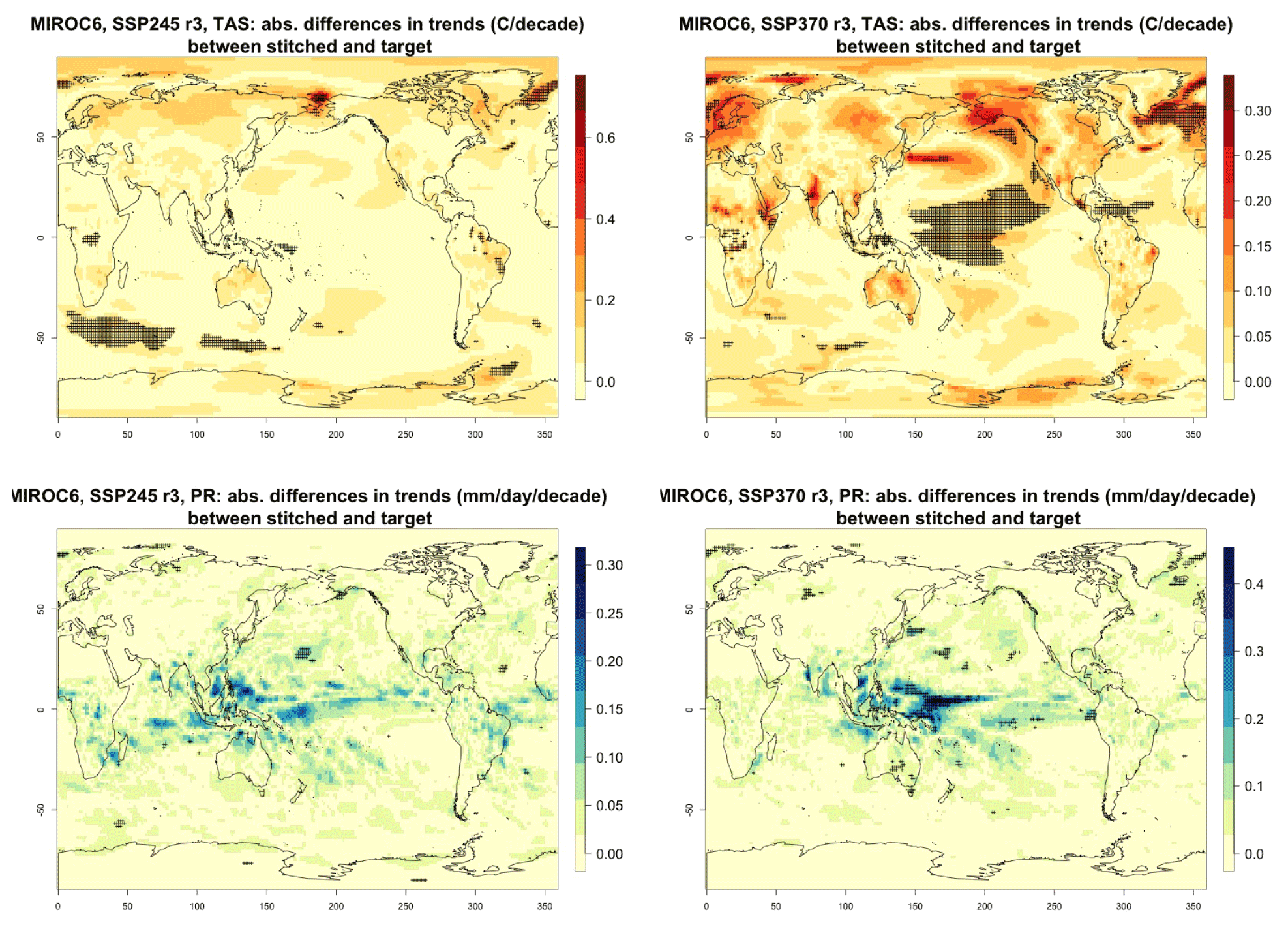
Figure C3 Absolute difference in decadal trends of temperature (TAS) and precipitation (PR) between stitched and target realizations. The value of the difference is expressed by the color scale, and we marked as significant with black crosses those locations where the 95 % confidence intervals of the trends computed from target and stitched time series do not overlap, indicating statistically significant differences. Emulation of MIROC6, monthly time series over 2015–2100, for SSP2-4.5 and SSP3-7.0. Third realization.

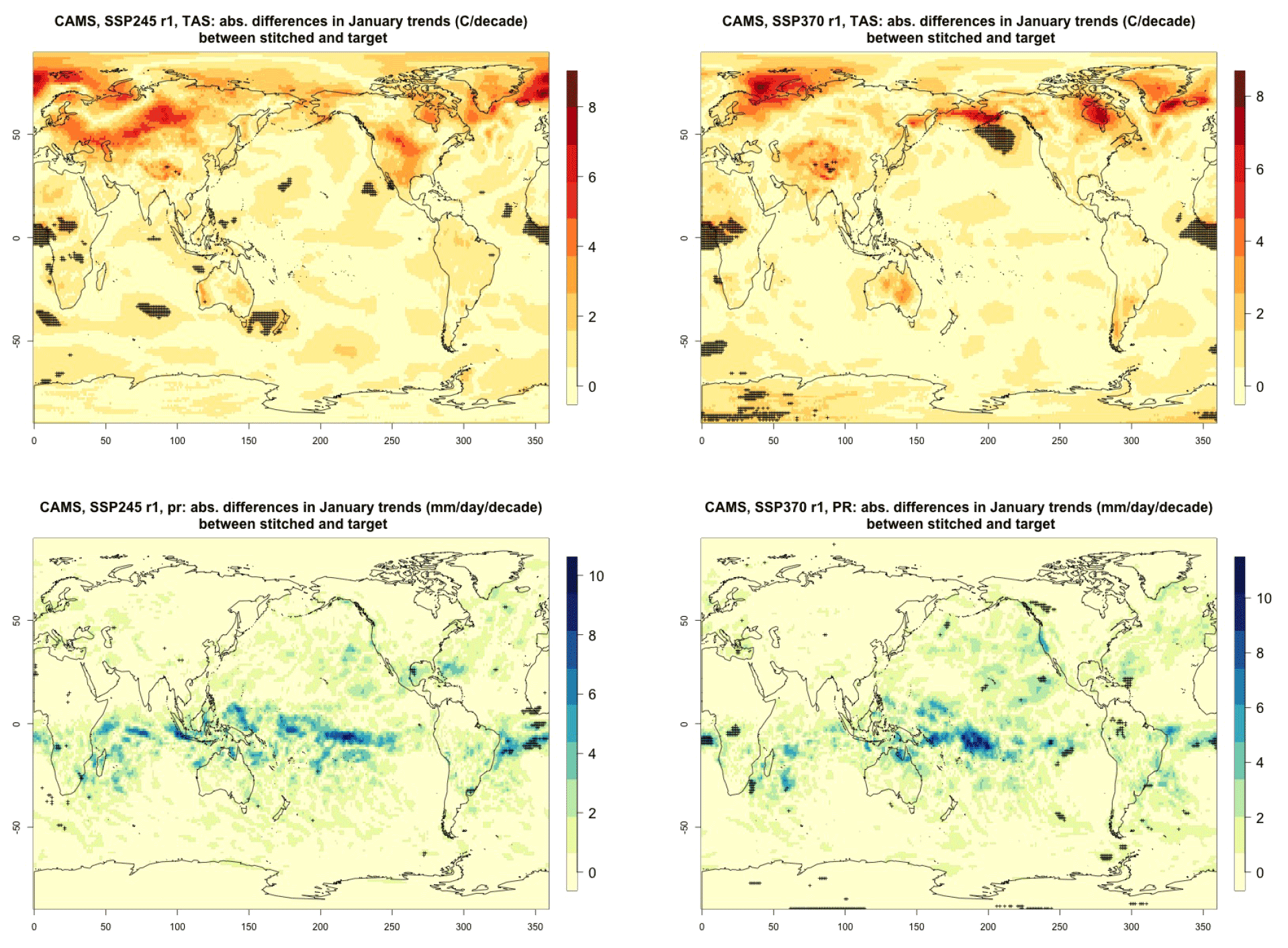
Figure C4 Absolute difference in decadal trends of January temperature (TAS) and precipitation (PR) between stitched and target realizations. The value of the difference is expressed by the color scale, and we marked as significant with black crosses those locations where the 95 % confidence intervals of the trends computed from target and stitched time series do not overlap, indicating statistically significant differences. Emulation of CAMS, January time series over 2015–2100, for SSP2-4.5 and SSP3-7.0.

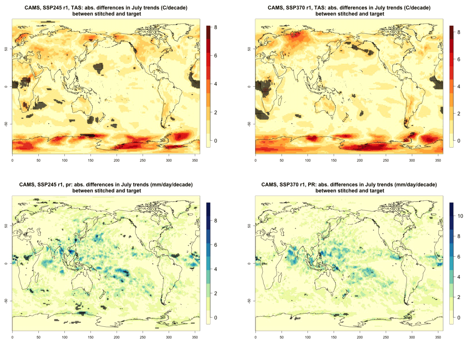
Figure C5 Absolute difference in decadal trends of July temperature (TAS) and precipitation (PR) between stitched and target realizations. The value of the difference is expressed by the color scale, and we marked as significant with black crosses those locations where the 95 % confidence intervals of the trends computed from target and stitched time series do not overlap, indicating statistically significant differences. Emulation of CAMS, July time series over 2015–2100, for SSP2-4.5 and SSP3-7.0.

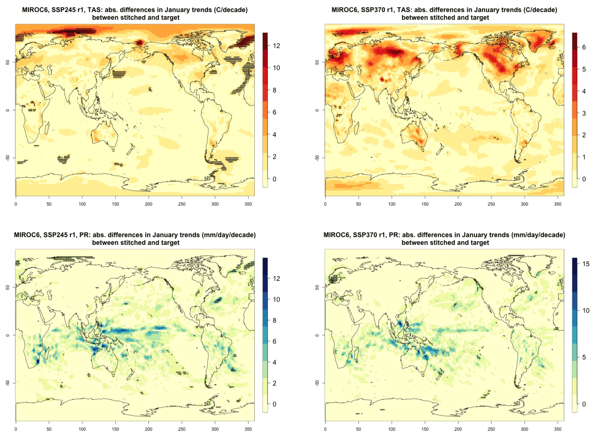
Figure C6 Absolute difference in decadal trends of January temperature (TAS) and precipitation (PR) between stitched and target realizations. The value of the difference is expressed by the color scale, and we marked as significant with black crosses those locations where the 95 % confidence intervals of the trends computed from target and stitched time series do not overlap, indicating statistically significant differences. Emulation of MIROC6, January time series over 2015–2100, for SSP2-4.5 and SSP3-7.0. First realization.

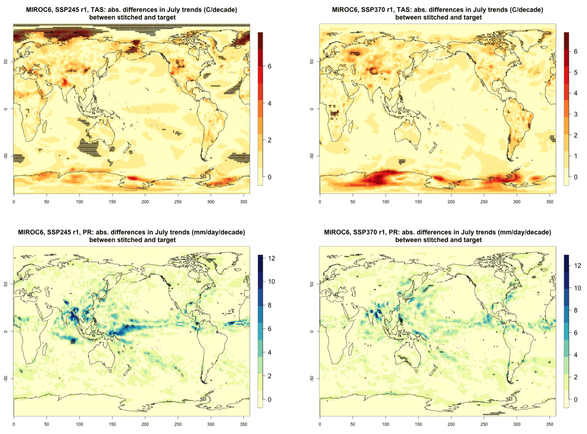
Figure C7 Absolute difference in decadal trends of July temperature (TAS) and precipitation (PR) between stitched and target realizations. The value of the difference is expressed by the color scale, and we marked as significant with black crosses those locations where the 95 % confidence intervals of the trends computed from target and stitched time series do not overlap, indicating statistically significant differences. Emulation of MIROC6, July time series over 2015–2100, for SSP2-4.5 and SSP3-7.0. First realization.

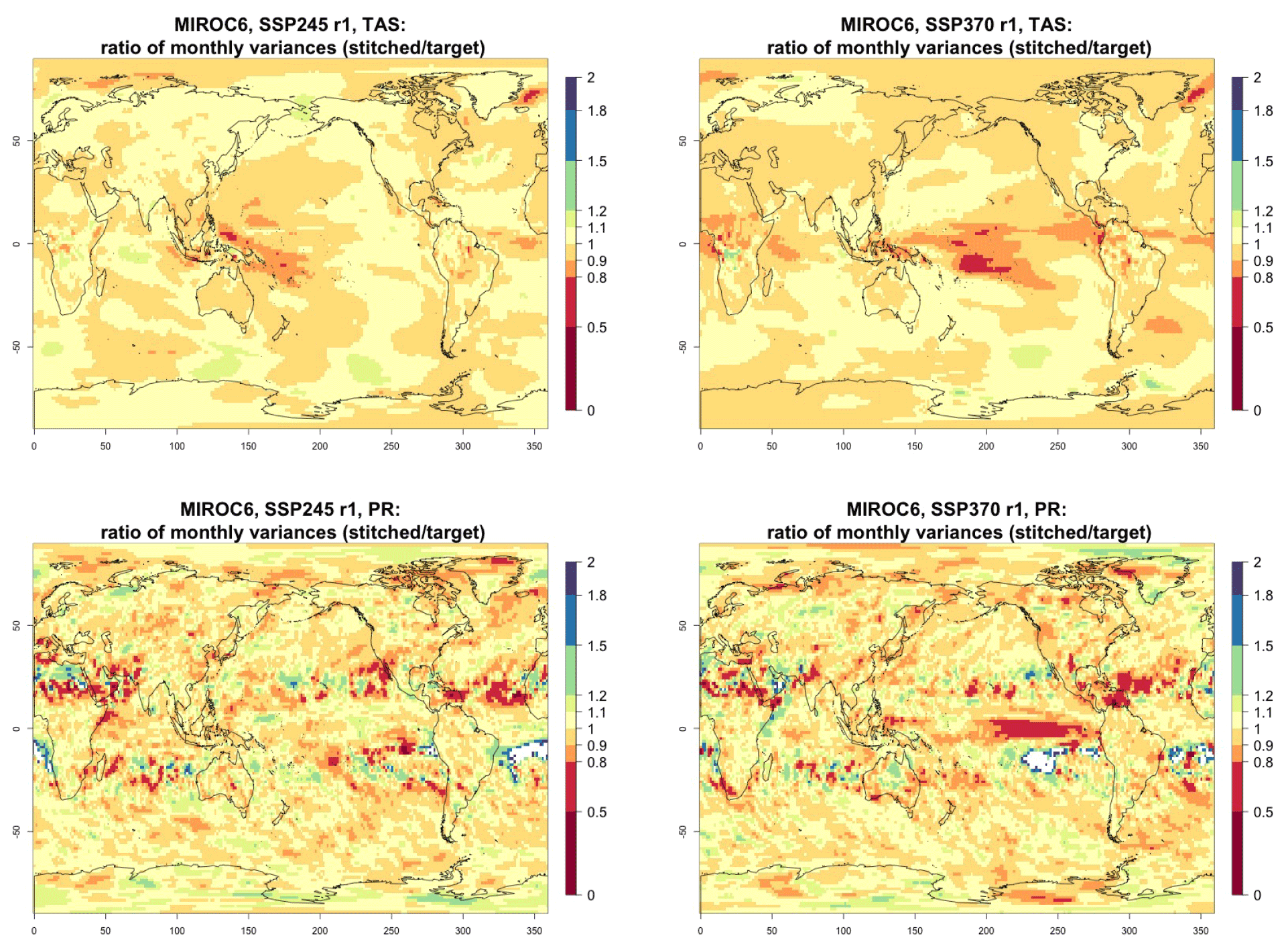
Figure C8 Ratio of monthly variability (standard deviation of residuals from trends) in temperature (TAS) and precipitation (PR) between stitched (at the numerator) and target (at the denominator) time series. The value of the ratio is expressed by the color scale, which highlights the transitions at 0.8 and 1.2. Emulation of MIROC6, monthly time series over 2015–2100, for SSP2-4.5 and SSP3-7.0. First realization.

Figure C9 Ratio of monthly variability (standard deviation of residuals from trends) in temperature (TAS) and precipitation (PR) between stitched (at the numerator) and target (at the denominator) time series. The value of the ratio is expressed by the color scale, which highlights the transitions at 0.8 and 1.2. Emulation of MIROC6, monthly time series over 2015–2100, for SSP2-4.5 and SSP3-7.0. Second realization.

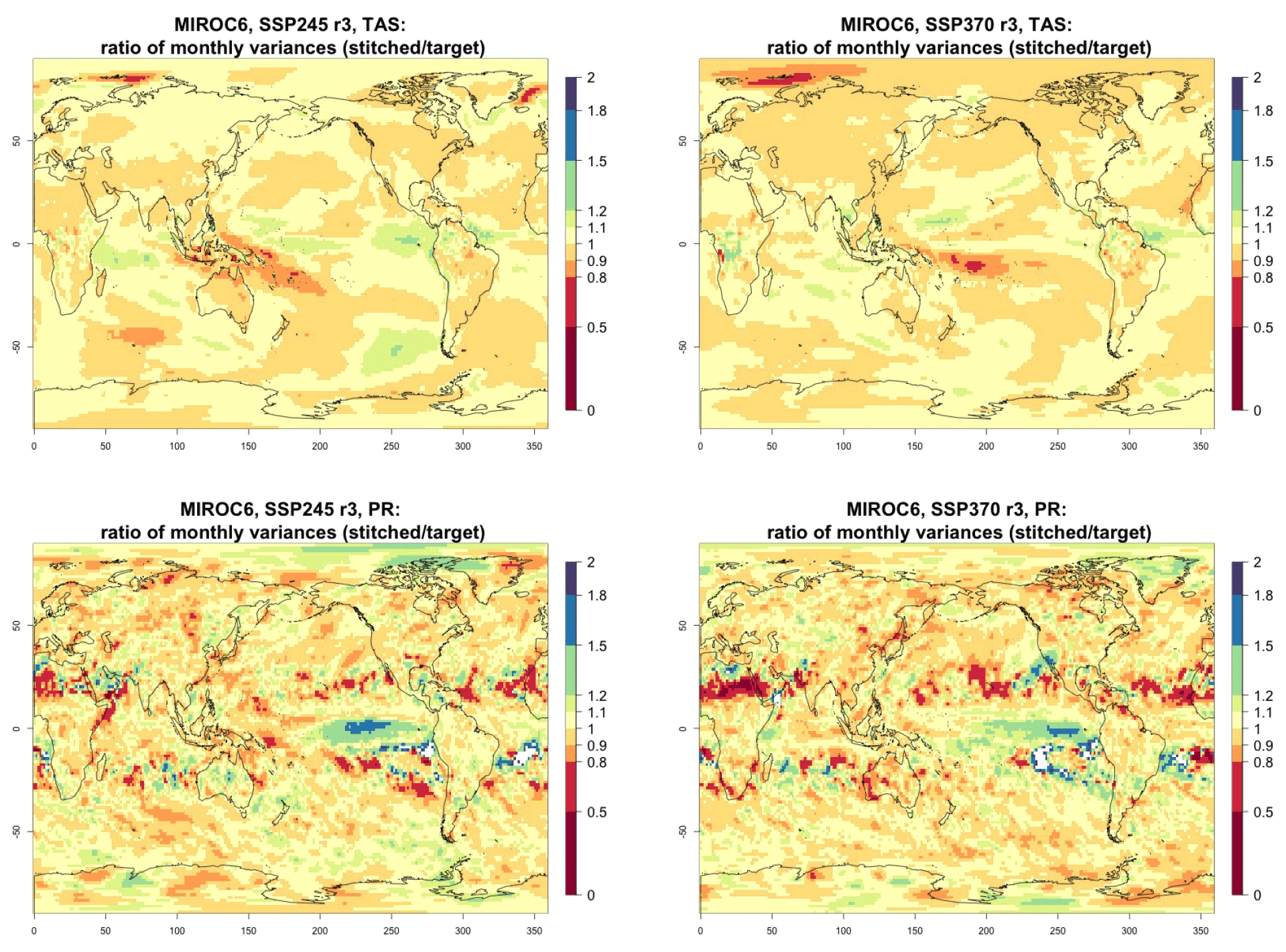
Figure C10 Ratio of monthly variability (standard deviation of residuals from trends) in temperature (TAS) and precipitation (PR) between stitched (at the numerator) and target (at the denominator) time series. The value of the ratio is expressed by the color scale, which highlights the transitions at 0.8 and 1.2. Emulation of MIROC6, monthly time series over 2015–2100, for SSP2-4.5 and SSP3-7.0. Third realization.

Appendix D: Additional SOI analysis for MIROC6

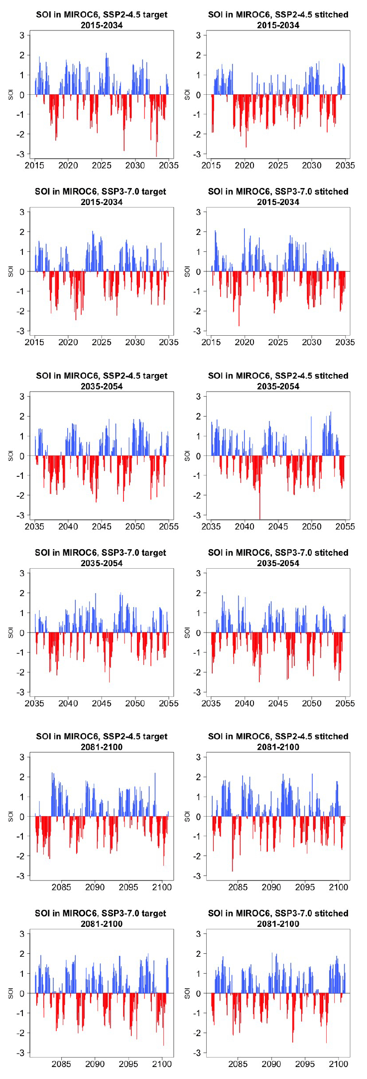
Figure D1 Examples of target (left) and stitched (right) SOI time series for three 20-year windows along the length of the simulation: 2015–2034 in the top four panels, 2035–2054 in the middle four panels, 2081–2100 in the bottom four panels. Results from emulation of SSP2-4.5 and SSP3-7.0 for one of three ensemble members emulated under each scenario for MIROC6.

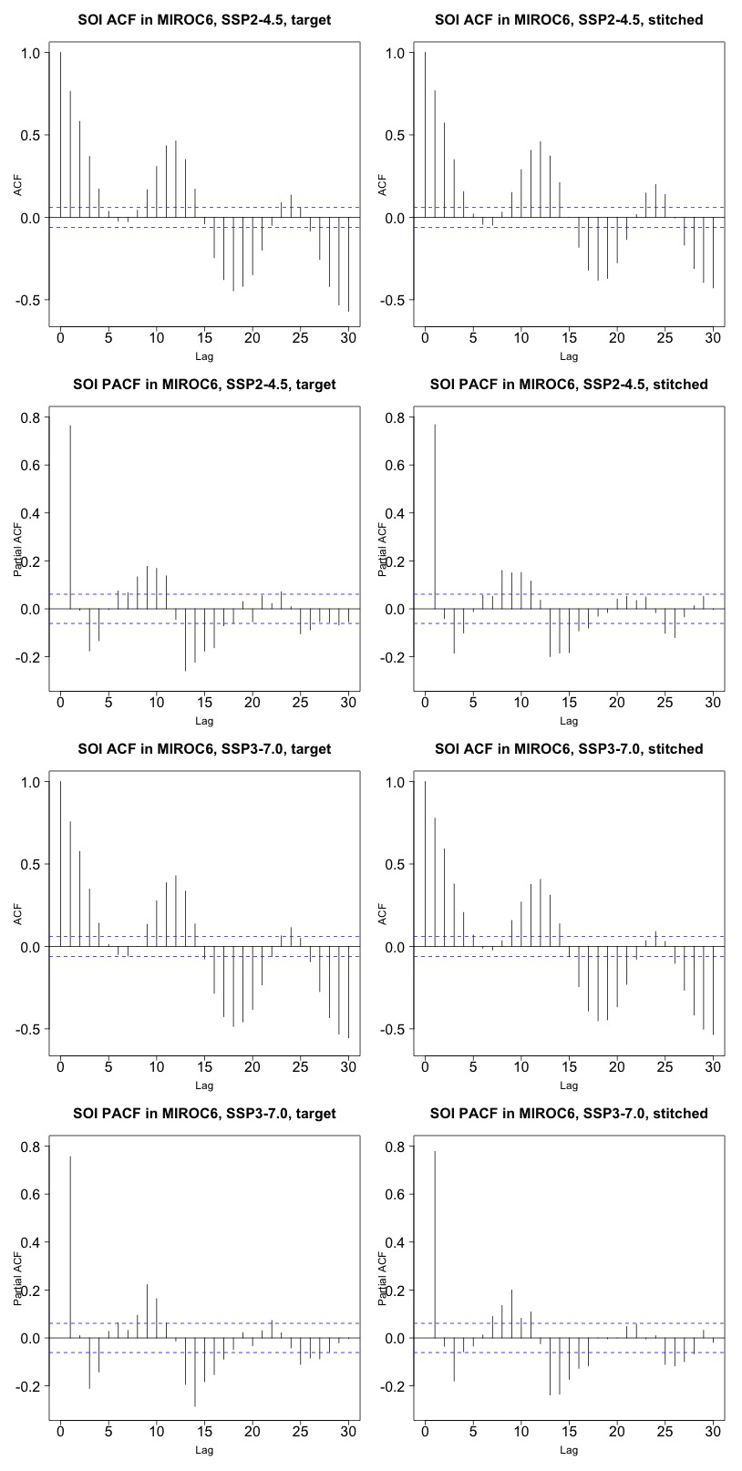
Figure D2 Auto-correlation functions (ACFs) and partial auto-correlation functions (PACFs) for real and stitched SOI time series. Top two rows: SSP2-4.5 ACF for target and stitched series and respective PACFs. Bottom two rows: SSP3-7.0 ACF for target and stitched series and respective PACFs. Results from emulation of one of three ensemble members emulated under each scenario for MIROC6. (Our software – R function acf(..,type="partial") – does not define the PACF at lag zero.)

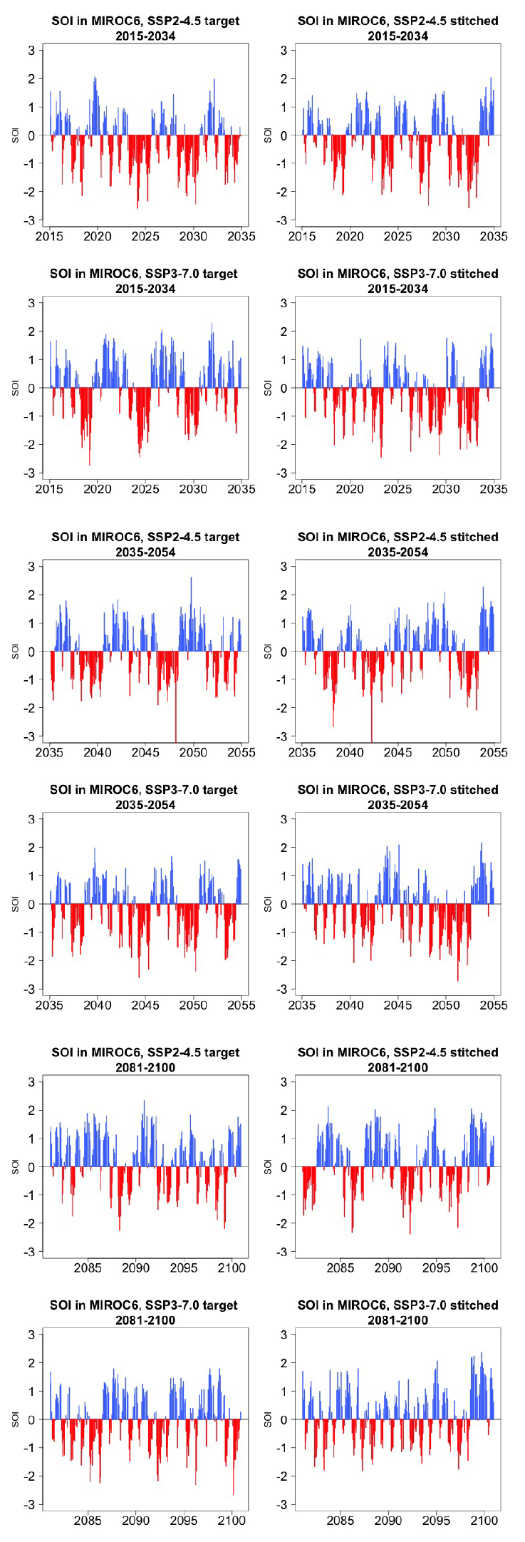
Figure D3 Examples of target (left) and stitched (right) SOI time series for three 20-year windows along the length of the simulation: 2015–2034 in the top four panels, 2035–2054 in the middle four panels, 2081–2100 in the bottom four panels. Results from emulation of SSP2-4.5 and SSP3-7.0 for one of three ensemble members emulated under each scenario for MIROC6.

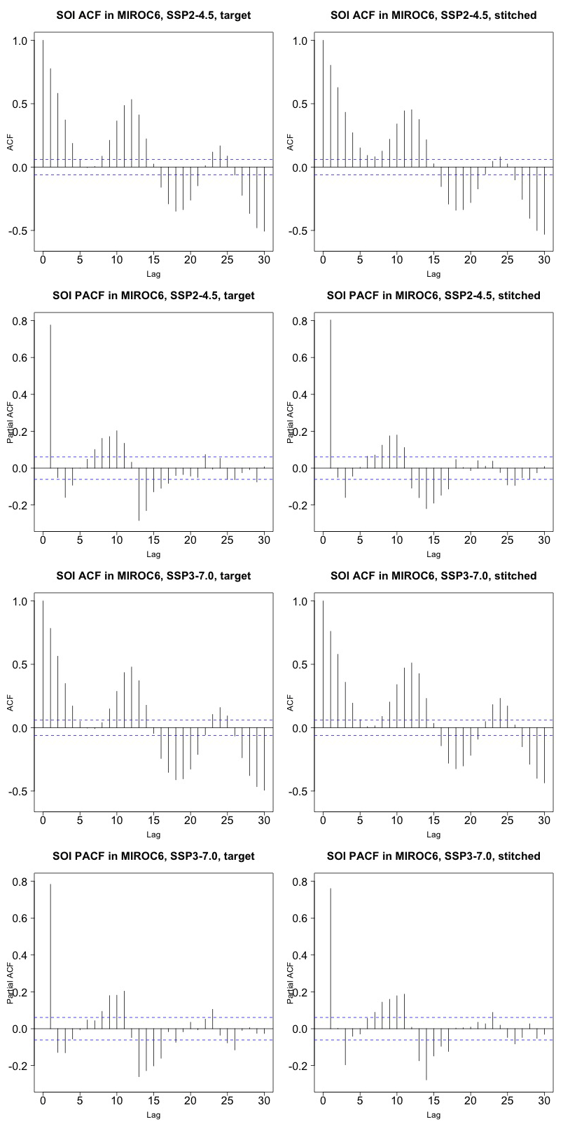
Figure D4 Auto-correlation functions (ACFs) and partial auto-correlation functions (PACFs) for real and stitched SOI time series. Top two rows: SSP2-4.5 ACF for target and stitched series and respective PACFs. Bottom two rows: SSP3-7.0 ACF for target and stitched series and respective PACFs. Results from emulation of one of three ensemble members emulated under each scenario for MIROC6. (Our software – R function acf(..,type="partial") – does not define the PACF at lag zero.)

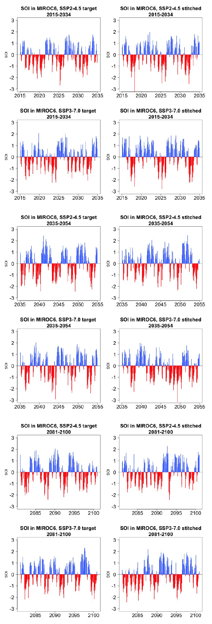
Figure D5 Examples of target (left) and stitched (right) SOI time series for three 20-year windows along the length of the simulation: 2015–2034 in the top four panels, 2035–2054 in the middle four panels, 2081–2100 in the bottom four panels. Results from emulation of SSP2-4.5 and SSP3-7.0 for one of three ensemble members emulated under each scenario for MIROC6.

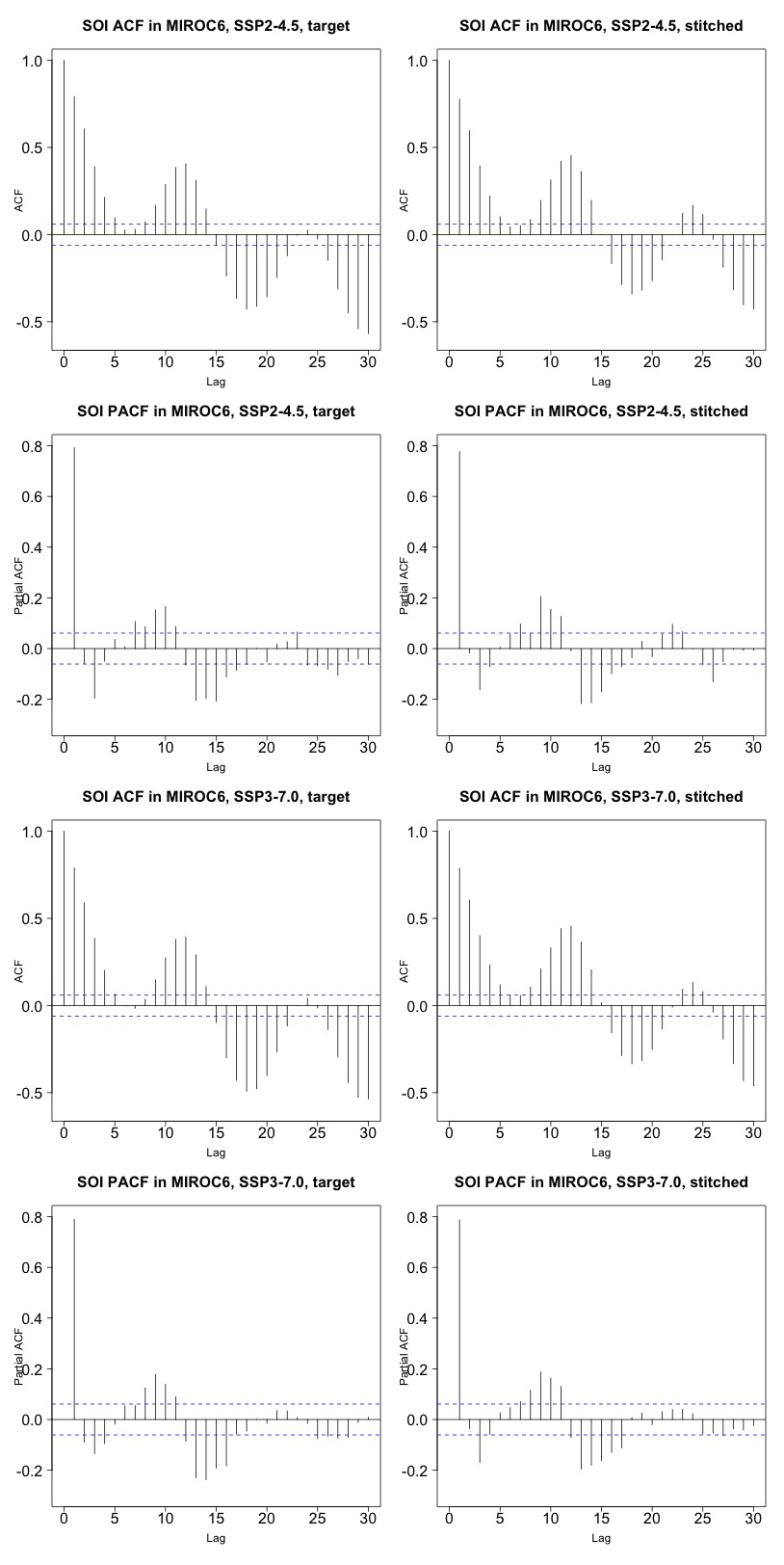
Figure D6 Auto-correlation functions (ACFs) and partial auto-correlation functions (PACFs) for real and stitched SOI time series. Top two rows: SSP2-4.5 ACF for target and stitched series and respective PACFs. Bottom two rows: SSP3-7.0 ACF for target and stitched series and respective PACFs. Results from emulation of one of three ensemble members emulated under each scenario for MIROC6. (Our software – R function acf(..,type="partial") – does not define the PACF at lag zero.)

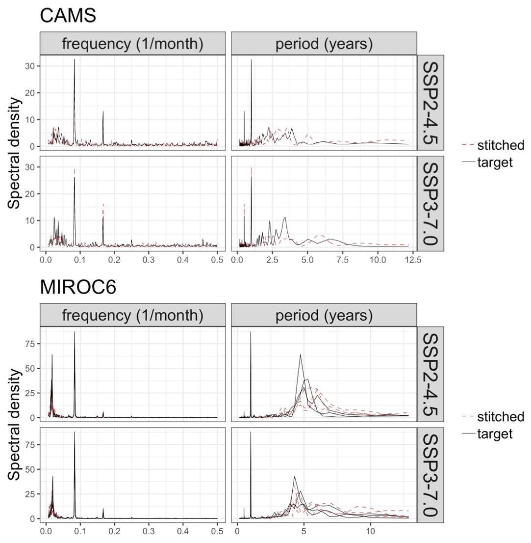
Figure D7 Spectral densities computed from target (solid lines) and stitched (dashed lines) SOI time series, for both models and one (for CAMS-CM-0, top four plots) and three (for MIROC6, bottom four plots) realizations.

Appendix E: GSAT time series for enriched ensembles

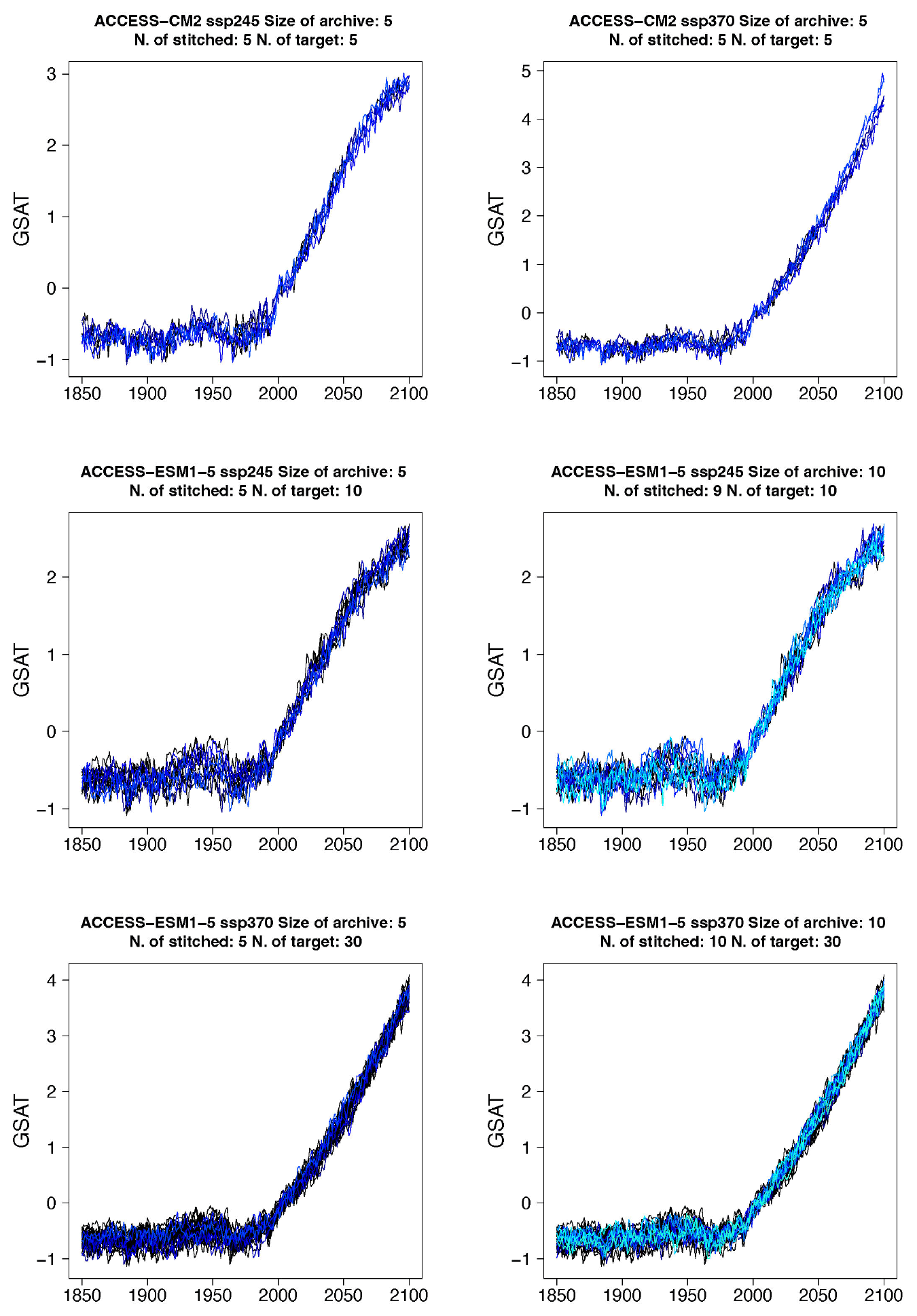
Figure E1 Examples of enriched ensembles of GSAT time series for ESMs in the PANGEO archive that have at least five trajectories available over the 21st century. As in the figures in Appendix A, warmer colors indicate a larger number of stitched trajectories in the figure, as the title also describes.

Figure E2 Examples of enriched ensembles of GSAT time series for ESMs in the PANGEO archive that have at least five trajectories available over the 21st century. As in the figures in Appendix A, warmer colors indicate a larger number of stitched trajectories in the figure, as the title also describes.

Figure E3 Examples of enriched ensembles of GSAT time series for ESMs in the PANGEO archive that have at least five trajectories available over the 21st century. As in the figures in Appendix A, warmer colors indicate a larger number of stitched trajectories in the figure, as the title also describes.

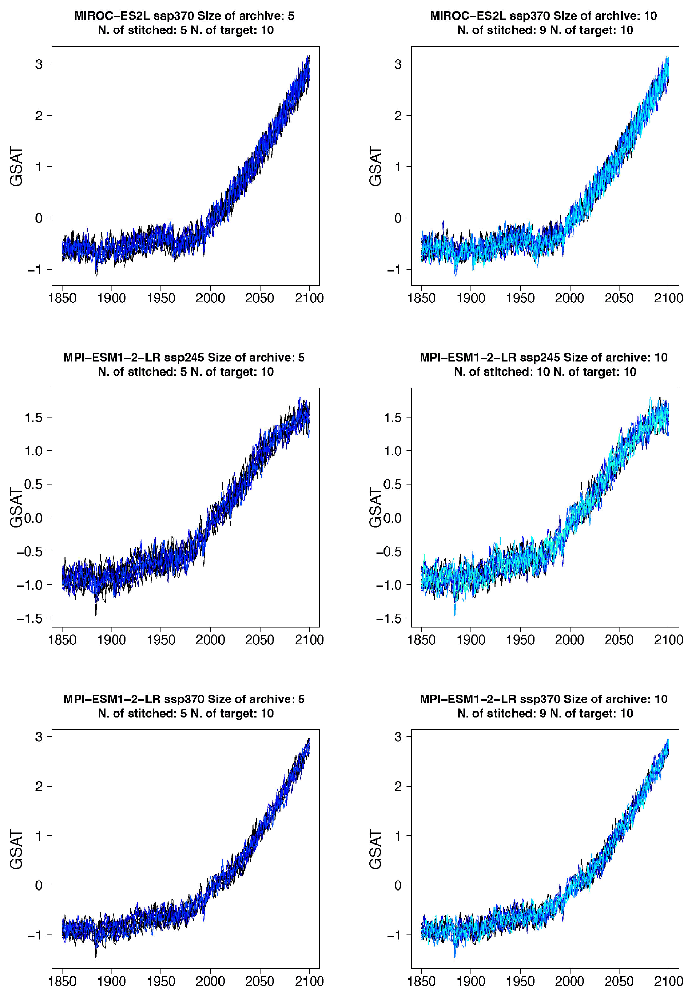
Figure E4 Examples of enriched ensembles of GSAT time series for ESMs in the PANGEO archive that have at least five trajectories available over the 21st century. As in the figures in Appendix A, warmer colors indicate a larger number of stitched trajectories in the figure, as the title also describes.

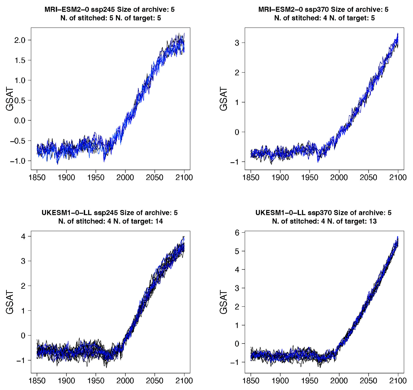
Figure E5 Examples of enriched ensembles of GSAT time series for ESMs in the PANGEO archive that have at least five trajectories available over the 21st century. As in the figures in Appendix A, warmer colors indicate a larger number of stitched trajectories in the figure, as the title also describes.

Appendix F: Table of E₁ and E₂ metrics for enriched ensemble exercise performed using only bracketing scenarios SSP1-2.6 and SSP5-8.5.

Table F1 The two components of the E_r metric, E₁ and E₂, computed for several experiments across ESMs, scenarios, and number of available archive trajectories from which to create the stitched ensembles. Numbers in columns 4 through 9 represent fractions of the target ensemble standard deviation (see Eq. 1).