Investigation of the extreme wet–cold compound events changes between 2025–2049 and 1980–2004 using regional simulations in Greece

This paper aims to study wet–cold compound events (WCCEs) in Greece for the wet and cold season November–April since these events may affect directly human activities for short or longer periods, as no similar research has been conducted for the country studying the past and future development of these compound events. WCCEs are divided into two different daily compound events, maximum temperature– (TX) accumulated precipitation (RR) and minimum temperature– (TN) accumulated precipitation (RR), using fixed thresholds (RR over 20 mm d⁻¹ and temperature under 0 ^∘C). Observational data from the Hellenic National Meteorology Service (HNMS) and simulation data from reanalysis and EURO-CORDEX models were used in the study for the historical period 1980–2004. The ensemble mean of the simulation datasets from projection models was employed for the near future period (2025–2049) to study the impact of climate change on the occurrence of WCCEs under the Representative Concentration Pathways (RCPs) 4.5 and 8.5 scenarios. Following data processing and validation of the models, the potential changes in the distribution of WCCEs in the future were investigated based on the projected and historical simulations. WCCEs determined by fixed thresholds were mostly found over high altitudes with TN–RR events exhibiting a future tendency to reduce particularly under the RCP 8.5 scenario and TX–RR exhibiting similar reduction of probabilities for both scenarios.

1 Introduction

Extreme weather events and their linkage to climate change is a matter of high concern for many scientific groups (Zanocco et al., 2018; Konisky et al., 2016; Curtis et al., 2017). In the last decade, numerous scientific studies focused on the causes, frequency, and impacts of extreme compound events (e.g., Aghakouchak et al., 2020; Singh et al., 2021; Sadegh et al., 2018; Zscheischler et al., 2017, 2018; Zscheischler and Seneviratne, 2017). As mentioned in the Intergovernmental Panel on Climate Change report on “Managing the risks of extreme events and disasters to advance climate change adaptation” (IPCC SREX) (Field et al., 2012, p. 118), compound events are defined as (1) two or more extreme events occurring simultaneously or successively, (2) combinations of extreme events with underlying conditions that amplify the impact of the events, or (3) combination of events that are not themselves extremes but lead to an extreme event or impact when combined (Leonard et al., 2014).

Recent studies have been conducted on the examination of wet–cold compound events (WCCEs) that concern daily values of temperature and precipitation, and the correlation of these variables (Chukwudum and Nadarajah, 2022; Lhotka and Kyselý, 2022), while other studies focus on the occurrence of monthly WCCEs for the historical period (Wu et al., 2019; Lemus-Canovas, 2022). However, the purpose of this article is the study of fixed thresholds extreme WCCEs on daily basis in Greece during the historical period (1980–2004) and how the likelihood of these events will be affected by climate change, during the period 2025–2049. It has been reported that WCCEs affect the region of the Mediterranean Basin, including Greece (Zhang et al., 2021). Studies using only observational data at some locations (Lazoglou and Anagnostopoulou, 2019), or modeled data mostly over the broader region of the Mediterranean Sea (Vogel et al., 2021; Hochman et al., 2022; de Luca et al., 2020), concerning WCCEs have been conducted in the past, but not depicting analytically WCCEs in Greece, a country that as a part of the Mediterranean Basin is considered a “climate change hotspot” (Ali et al., 2022). This work attempts to fill this void on the effects of climate change on WCCEs in Greece.

The examined events belong to the first category of the definition of compound events from IPCC since they refer to the simultaneous exceedance of precipitation and temperature thresholds. WCCEs may have a negative impact on people's lives by causing electricity blackouts, affecting agriculture with heavy snowfall or freezing rain, and blocking transportation because of closed roads, railways, or even airports (Houston et al., 2006; Llasat et al., 2014; Vajda et al., 2014). On the other hand, most of the available freshwater in the country comes from melted mountain snow during spring or summer. Finally, eco-systems, especially in mountains, may be affected by the absence of snow that climate change may cause (Demiroglu et al., 2015; Pestereva et al., 2012; Trujillo et al., 2012; García-Ruiz et al., 2011).

The first part of the study concerns the historical period between 1980 and 2004, because of the availability of quality-controlled daily observational data for minimum temperature (TN), maximum temperature (TX), and accumulated precipitation (RR). Hence, for that period, we use observational data from 21 Hellenic National Meteorological Service (HNMS) stations, to validate EURO-CORDEX regional climate models (RCMs), provided by the Copernicus Climate Change Service and the projection model dataset produced in-house. In addition to the models, two reanalysis products are included as the closest to “true” past climate conditions in regions with no or scarce observations (Moalafhi et al., 2016). More information about the observational and model datasets is presented in Sect. 2. Section 3 highlights the applied methodology while Sect. 4 displays WCCEs observed in stations and station cells of the models, and Sect. 5 discusses the reanalysis and projections ensemble mean WCCEs probabilities spatial distribution for the historical period. Section 6 details the results of the difference in WCCEs probabilities between the historical and the near future period between 2025 and 2049 for two greenhouse gas concentration scenarios, RCP4.5 and RCP8.5.

2 Data

In this section, we present the datasets that provide the observational and simulation data produced by projection and reanalysis models.

2.1 HNMS observations

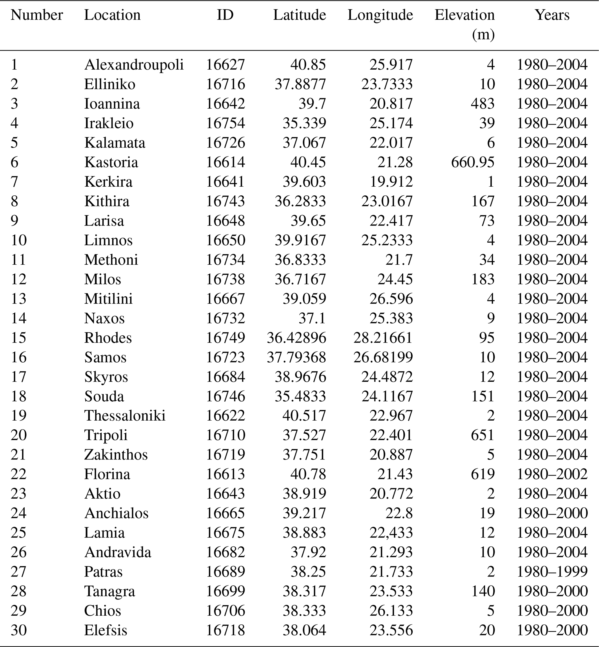
HNMS freely provides observational data from 21 stations for the purpose of scientific research (http://www.emy.gr/emy/el/services/paroxi-ipiresion-elefthera-dedomena, last access: 1 March 2021). The data have been formally evaluated by HNMS and the time series shows no missing or distorted values. In particular, the time series' available for the historical period 1980–2004 have a 3 h temporal resolution, and from these values we have extracted the daily values of TN, TX, and RR. Moreover, stations 22–30 which also belong to the network of HNMS stations contain observations in the period 1980–2004, although none of the stations covers all observational days in the period. The datasets of these stations were extracted by the National Centers for Environmental Information of National Oceanic and Atmospheric Administration. We selected stations that contain at least 20 years of observations. Figure 1 shows the position of the stations on the orography of ERA5 and WRF, while Table A1 of the Appendix provides details on the characteristics of the stations. We have used observational data to validate the model datasets regarding the WCCEs for the historical period.

Figure 1 Map of HNMS stations on orography of (a) ERA5 and (b) WRF-ERA-Interim. The numbers correspond to those in Table A1.

2.2 Reanalysis models

We have used two reanalysis models due to the lack of spatially and temporally complete direct observations, to study consistently the WCCEs in Greece in the historical period. The first model is the latest available reanalysis product ERA 5 from the European Centre for Medium-range Weather Forecasts (ECMWF) of spatial resolution ∼30 km × 30 km (Hersbach et al., 2020). The second reanalysis model, built in the Environmental Research Laboratory (EREL) of the National Center of Scientific Research “Demokritos” (NCSRD) WRF_ERA_I, has been produced by dynamically downscaling ERA-Interim using the Weather Research Forecast (WRF) model (v3.6.1) from 80 km × 80 km to 5 km × 5 km (Politi et al., 2048, 2020, 2021).

Table 1 EURO-CORDEX and EREL-NCSRD simulation models information.

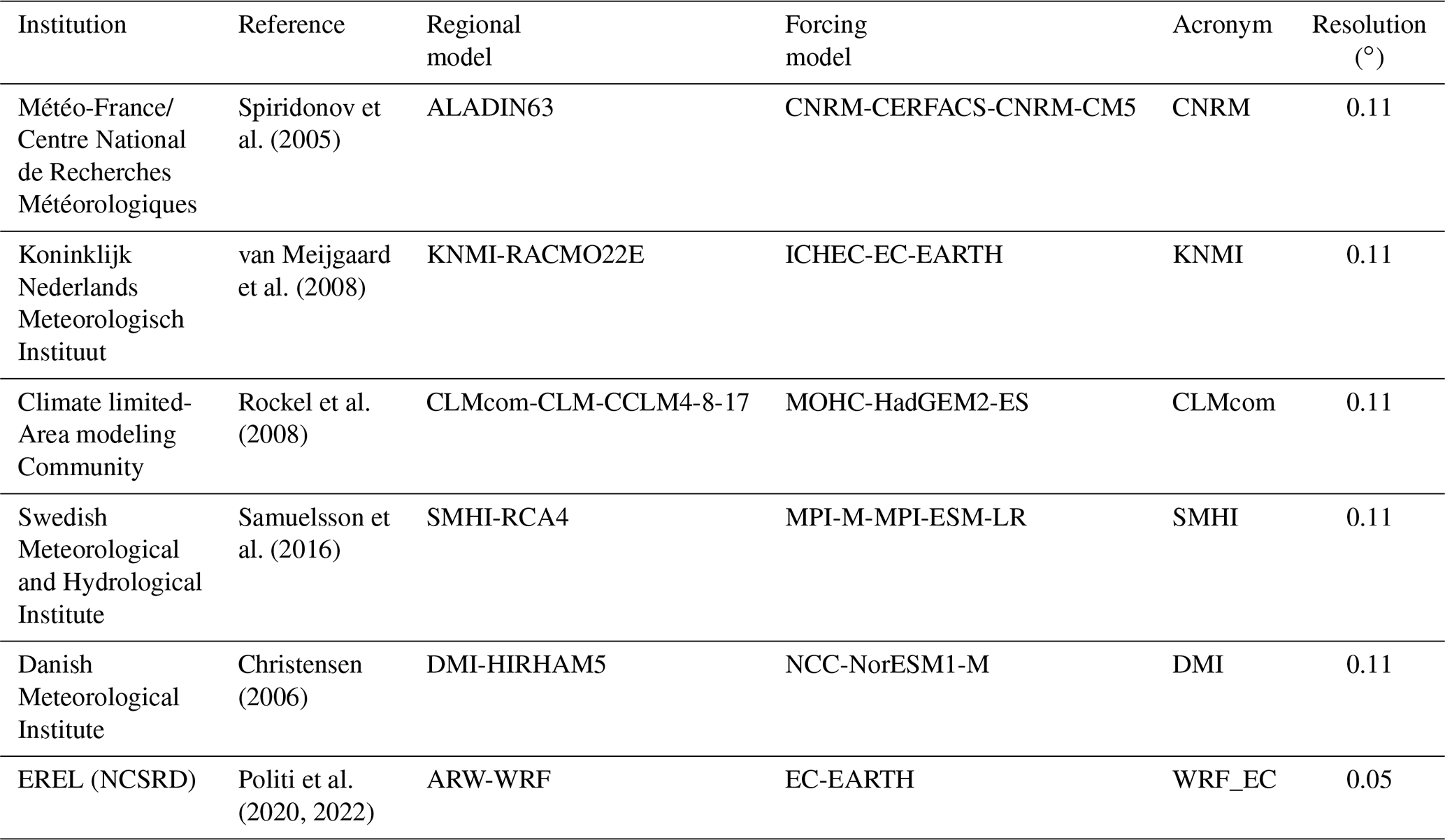
2.3 GCM/RCM models

To observe possible alterations of WCCEs occurrence probability in the future period 2025–2049 compared to the historical period, we employed data from RCM simulations driven by GCMs. In this regard, we obtained data from five models included in the EURO-CORDEX initiative provided by the Copernicus Program. All chosen EURO-CORDEX models with available daily data for both RCP scenarios were selected because they have the finest spatial resolution of $\mathrm{0.11}{}^{\circ }\times \mathrm{0.11}{}^{\circ }$, and have also been tested in Cardoso et al. (2019). Information on the regional and parent models and their acronyms used herewith is given in Table 1. In addition to the EURO-CORDEX model data, we have used dynamically downscaled data from the EC-EARTH GCM to a high spatial resolution of 5 km × 5 km for the area of Greece using the WRF model (Politi et al., 2020, 2022).

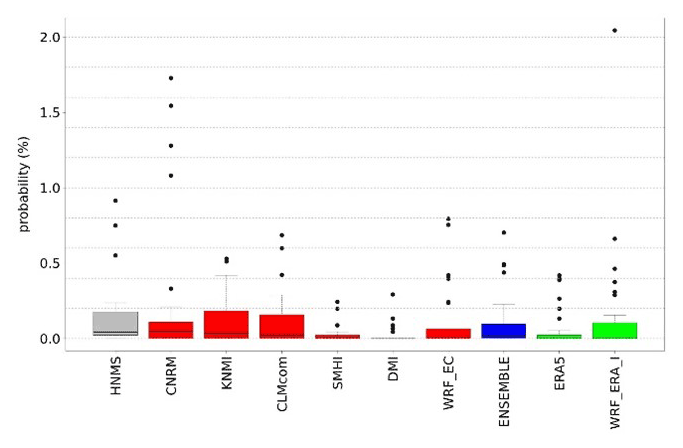
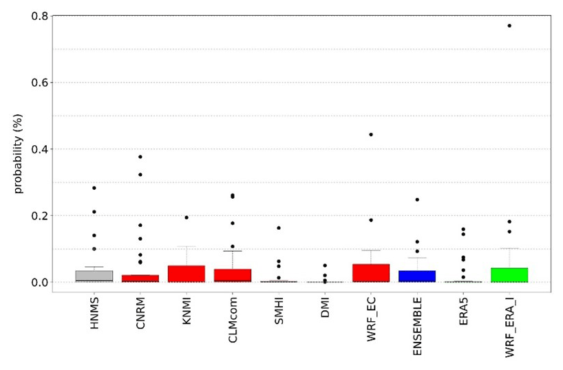
Figure 2 Box plot presenting RR20FD empirical method probabilities for observations and models.

Figure 3 Box plot presenting RR20FD copula method probabilities for observations and models.

3 Methodology

The first step in this study is the validation of the projection and reanalysis models against observations. Moreover, the ensemble of the six projection models is also exhibited. We choose, as the ensemble resolution, that of the CORDEX models, since five of them share the same spatial resolution. The only model in need of regridding is WRF_EC. We follow the nearest neighbor method to upscale WRF_EC from 5 to 11 km. In addition, we use box plots to depict the ability of the models to simulate observational data WCCEs probabilities for the historical period at the cells that include meteorological stations. The box plots consist of the colored box, where in the band near the middle of the box is the median, bottom, and top of each color box are the 25th (Q₁) and 75th (Q₃) percentiles (BL). The lower limit of the whisker (LLW) is calculated by LW = Q₁ − 1.5 × BL and the upper limit (ULW) by UW = Q₃ + 1.5 × BL. The length of the whiskers (WL) is calculated as the difference between ULW and LLW. Any value out of this range is marked by a black point in the plot. The validation is conducted after the elevation bias correction of temperature at the cells of the models containing the stations. The cells of the stations are found using the nearest neighbor approach and the temperature bias correction temperature is the following:

$$\begin{array}{}\text{(1)}& T_{\mathrm{s}}=T_{\mathrm{m}}+\mathrm{0.006}\cdot \left(H_{\mathrm{m}}-H_{\mathrm{s}}\right).\end{array}$$

In Eq. (1), T_s is the temperature of the cell after the elevation bias correction, T_m is the temperature provided by the model, H_m is the cell elevation, and H_s is the elevation of the HNMS station.

3.1 Compound event selection

According to HNMS, the meteorological year can be split into two climate periods (http://emy.gr/emy/el/climatology/climatology, last access: 1 February 2022). The cold and wet period extends on average from mid-October to the end of March, and the warm–dry period occurs during the rest of the year. Since the study is focused on the extreme WCCEs, we examine the period between November and April, since according to the HNMS observations, April exhibits lower temperatures than October and more rainy days. Moreover, it is not uncommon for the northern parts of Greece, especially mountainous areas, to be affected by snowfalls during April. This leads to the creation of a time series of 4532 daily values for the historical period and 4531 for the future period. CLMcom considers that each month consists of 30 d, thus leading to 4500 values for each period. Also, DMI considers that a calendar year has 365 d, thus each period examined has 4525 values.

The WCCEs, which are examined on a daily basis, are divided into two types of synchronous events, TX–RR and TN–RR, and studied using the fixed threshold approach (Table 2). This approach considers the fixed threshold of 20 mm d⁻¹ for RR and 0 ^∘C for TN and TX for all stations or grid points, as recommended by the Commission for Climatology (CCl), the World Climate Research Programme (WCRP) of the Climate Variability and Predictability Component (CLIVAR), project and the Expert Team for Climate Change Detection and Indices (ETCCDI). TN equal to or under 0 ^∘C indicates Frost Days (FD), while TX equal to or under 0 ^∘C indicates Iced Days (ID) (Fonseca et al., 2016). The thresholds examined have been proposed in various works for studying extreme events (Raziei et al., 2014; Tošić and Unkašević, 2013; Anagnostopoulou and Tolika, 2012; Pongrácz et al., 2009; Kundzewicz et al., 2006; Moberg et al., 2006).

Table 2 Univariate thresholds and the compound events examined in the study.

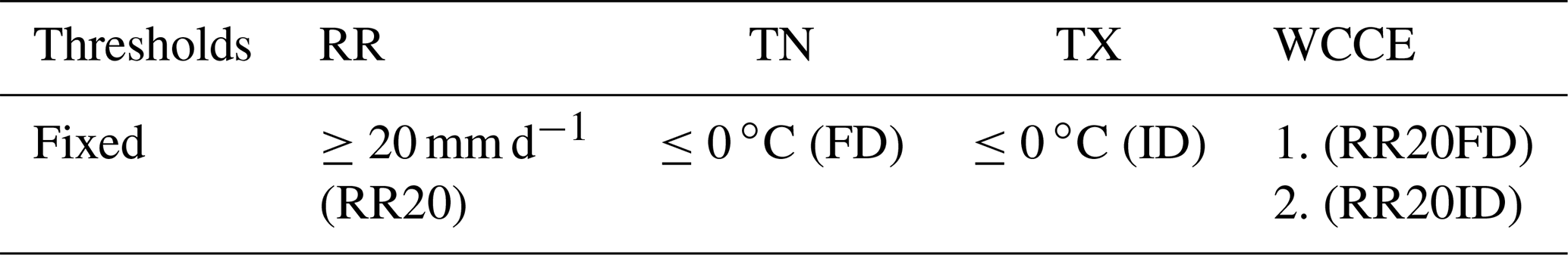
Table 3 Contingency table where “A” is the number of event forecasts that correspond to event observations or the number of hits. Entry “B” is the number of event forecasts that do not correspond to observed events or the number of false alarms. Entry “C” is the number of no-event forecasts corresponding to observed events or the number of misses. Entry “D” is the number of no-event forecasts corresponding to no events observed or the number of correct rejections.

3.2 WCCEs probability calculation

The WCCEs probabilities are calculated by applying two different methods. The first is the empirical approach counting the events from the time series and dividing by the total number of days to find the percentage (%) of the occurrence probability. For the second method, we use the copula approach for the HNMS observations and model comparison, and to map the differences between the two methods for the reanalysis and projection of model data. Compared to copula, an empirical method has a higher uncertainty when calculating the probability of extreme events (Hao et al., 2018; Tavakol et al., 2020; Zscheischler and Seneviratne, 2017). The purpose of using two different methods is to investigate whether the copula method underestimates or overestimates the WCCEs.

The best fitting copula selection for each time series is examined using the R programming language function BiCopSelect as suggested in Zhou et al. (2019), package VineCopula (Schepsmeier et al., 2013). The appropriate bivariate copula for each dataset is chosen by the function, from a multitude of 40 different copula families using the Akaike information criterion (AIC) (Akaike, 1974) and Bayesian information criterion (BIC), and the copula chosen for each station and model dataset is shown in the Supplement (Tables S5 and S6). Copulas are used in plenty of studies that investigate the dependence between two different climate variables and the joint probability of compound events (Tavakol et al., 2020; Dzupire et al., 2020; Pandey et al., 2018; Cong and Brady, 2012; Abraj and Hewaarachchi, 2021).

As mentioned in Nelsen (2007), a bivariate copula is a bivariate distribution function where margins are uniform on the unit interval [0, 1]. A bivariate copula is a map C: [0,1]² → [0, 1] with $C(u,\mathrm{1})=u$ and $C(\mathrm{1},v)=v$. Let X and Y be random variables with a joint distribution function $F(x,y)=\mathrm{Pr}(X\le x,Y\le y$) and continuous marginal distribution functions $F_{\mathrm{1}}\left(x\right)=\mathrm{Pr}(X\le x$) and $F_{\mathrm{2}}\left(y\right)=\mathrm{Pr}(Y\le y$), respectively. By Sklar's theorem (Sklar, 1959), one obtains a unique representation as follows:

$$\begin{array}{}\text{(2)}& F(x,y)=C\left\{F_{\mathrm{1}}\left(x\right),F_{\mathrm{2}}\left(y\right)\right\}.\end{array}$$

For the two random variables of X (e.g., precipitation) and Y (e.g., temperature) with cumulative distribution functions (CDFs) $F_{\mathrm{1}}\left(x\right)=\mathrm{Pr}(X\ge x$) and $F_{\mathrm{2}}\left(y\right)=\mathrm{Pr}(Y\le y$), the bivariate joint distribution function or copula (C) can be written as

$$\begin{array}{}\text{(3)}& F(x,y)=\mathrm{Pr}(X\ge x,Y\le y)=C(u,v).\end{array}$$

3.3 WCCEs assessment in HNMS stations

In this section, the models are validated against observations both for the empirical and the copula method. WCCEs probabilities for each station and model are presented in the Supplementary material. BIAS and RMSE along with the critical success index (CSI) are used for the validation. CSI is calculated as $\mathrm{CSI}=A/(A+B+C)$. A, B, and C symbolize elements from the contingency table (Table 3) that occur from comparing zero and non-zero probabilities in stations with the corresponding model cells. Also, the total number of events calculated for both methods from observational data is presented for each station.

3.4 RR20FD

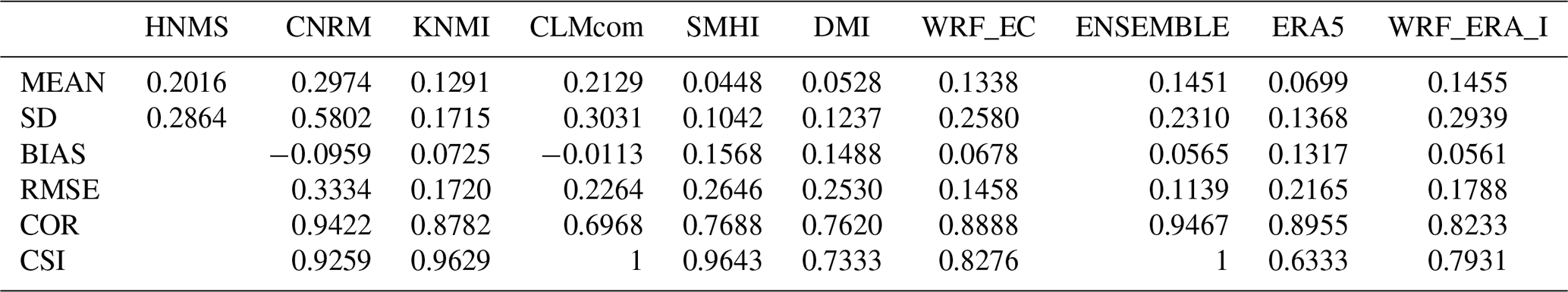
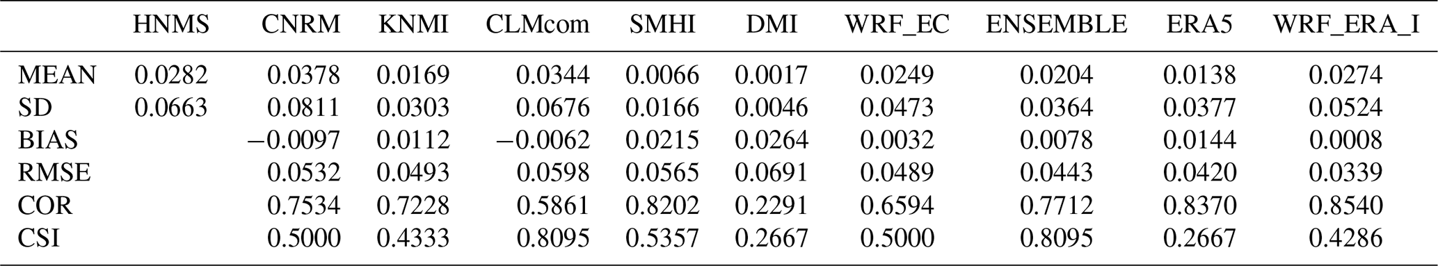
Probability values for each station are presented in the Supplement (Tables S1–S4) as well as the contingency tables (Tables S7–S10) from which CSI is calculated. ERA5 and WRF_ERA_I are reanalysis products and exhibited for comparison reasons. The copulas selected by Bicopselect for each observational and modeled time series are also presented in Tables S5 and S6. Figures 2 and 3 and Tables 4 and 5 show that most models and observations tend to yield higher probabilities for the copula than the empirical method.

Table 4 Table exhibiting mean (MEAN) station RR20FD empirical probabilities (%) for observations and models, standard deviation (SD), bias (BIAS), rmse (RMSE), Pearson correlation (COR), and CSI of models against observations.

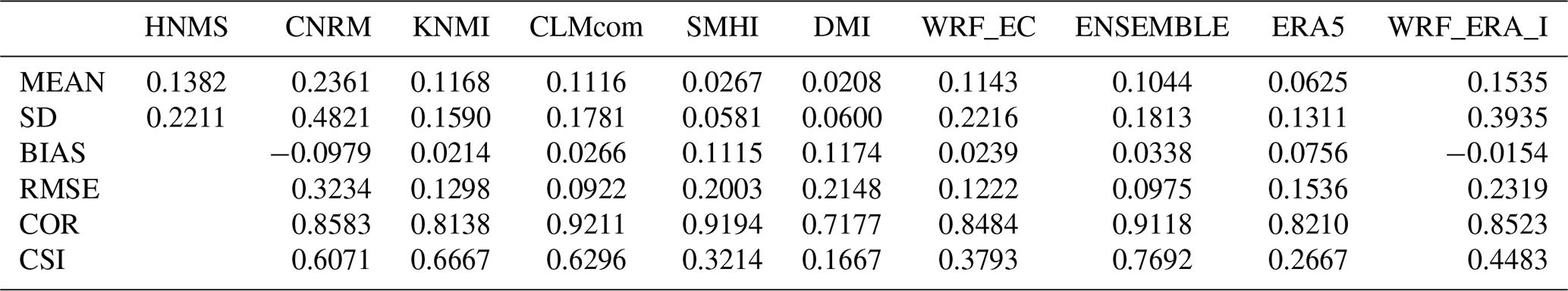
Table 5 Table exhibiting mean (MEAN) RR20FD copula station probabilities (%) for observations and models, standard deviation (SD), bias (BIAS), rmse (RMSE), Pearson correlation (COR), and CSI of models against observations.

3.5 RR20ID

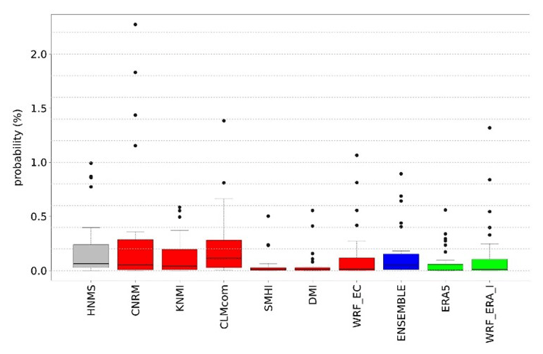
RR20ID events yield, as expected, lower probabilities than RR20FD events as observed in Figs. 4 and 5 and Tables 6 and 7. Most observations and models yield zero probabilities, hence validation of models for these events is limited. The empirical method exhibits eight stations with non-zero probabilities in the historical period (Supplement).

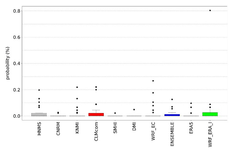
Figure 4 Box plot presenting RR20ID empirical method probabilities for observations and models.

Figure 5 Box plot presenting RR20ID copula method probabilities for observations and models.

3.6 Observations–models comparison conclusions

The events examined are rare among the available stations for the historical period. Copulas considering the dependence between the variables yield greater probabilities than the empirical method. More stations with non-zero probabilities enable more accurate validation of the models. To minimize uncertainties, smooth extreme underestimations or overestimations of WCCE probabilities that each model yields, and because ENSEMBLE shows better consistency among the projection models' statistical indices, we use it for further analysis in the study.

4 Historical period models WCCEs on maps

In this section, WCCEs spatial distribution probabilities are compared between empirical and copula methods. This procedure is conducted separately for the two reanalysis products and the Ensemble mean of the projection models.

4.1 Reanalysis

ERA5 and WRF_ERA_I WCCEs spatial distribution probabilities in Greece are displayed in this section. We display both reanalysis products, although ERA5 is the most recently developed reanalysis product, we exhibit also WRF_ERA_I since its much finer spatial resolution is more appropriate for the complex topography of Greece with many mountains and islands.

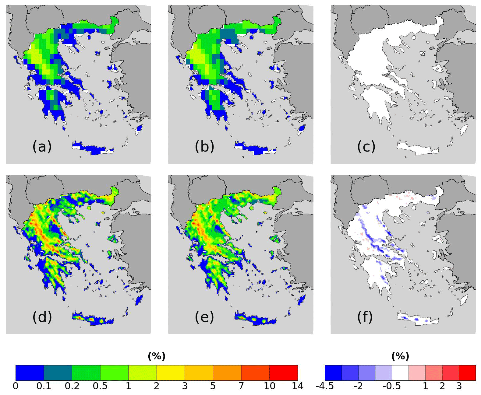
Figure 6 RR20FD probabilities for (a–c) ERA5 and (d–f) WRF_ERA_I produced by (a, d) empirical and (b, e) copula and =  (b)–(a) and (f) = (e)–(d).

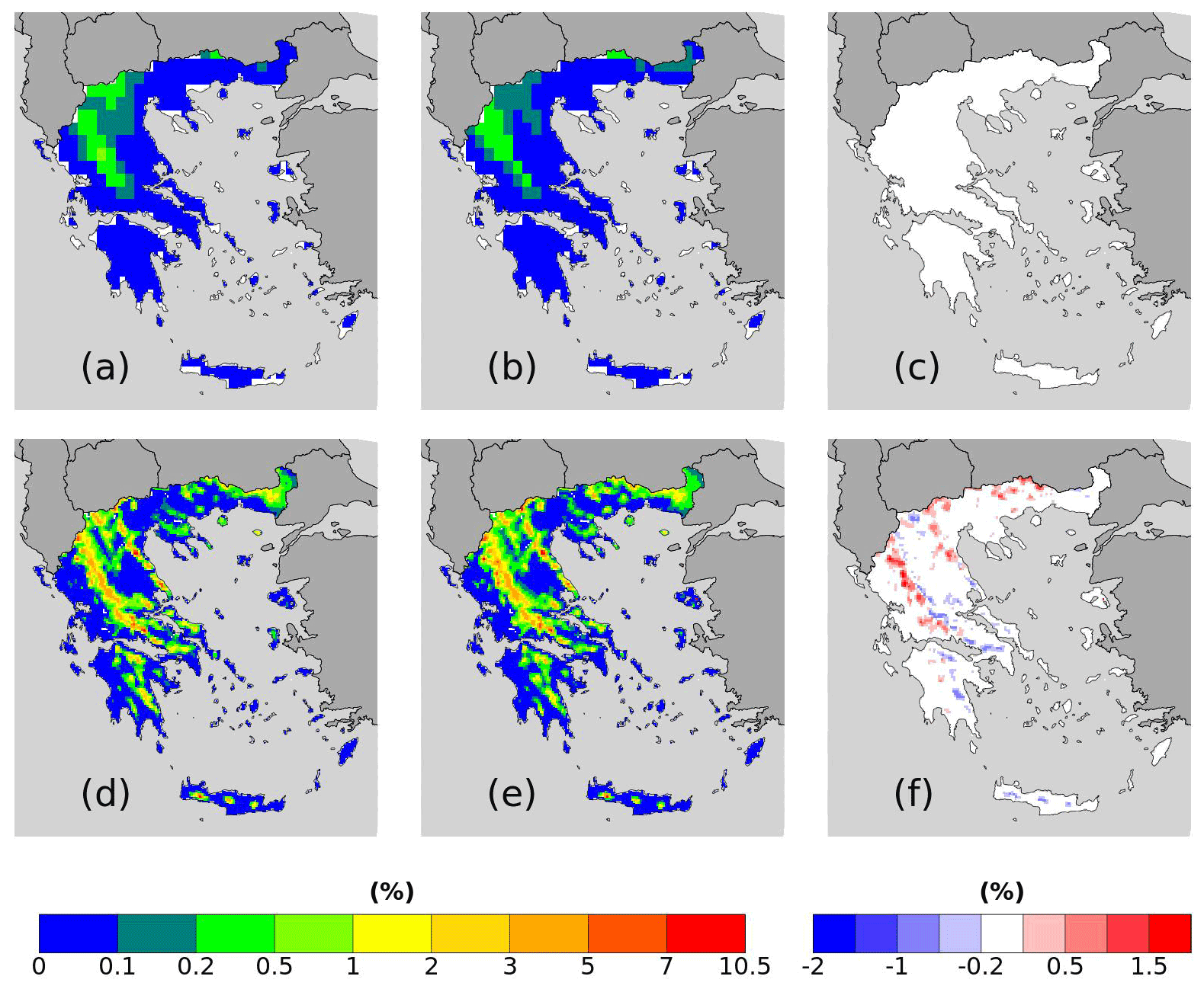
Figure 7 RR20ID probabilities for (a–c) ERA5 and (d–f) WRF_ERA_I produced by (a, d) empirical and (b, e) copula a (c) = (b)–(a) and (f) = (e)–(d).

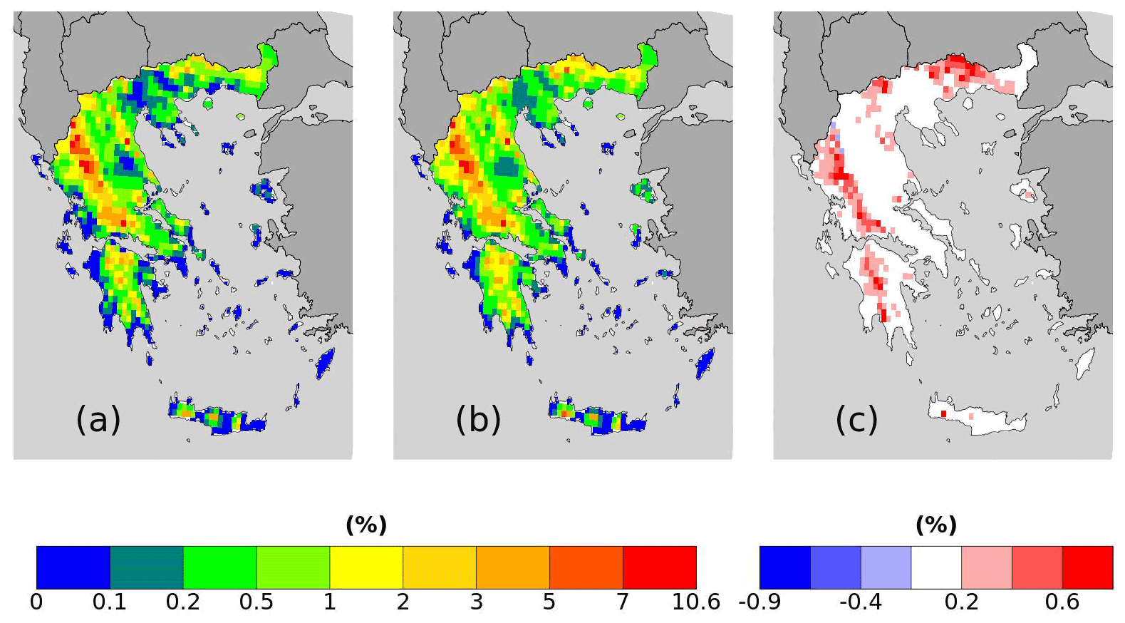
Figure 8 RR20FD ensemble probabilities for (a) empirical and (b) copula method. (c) = (b)–(a).

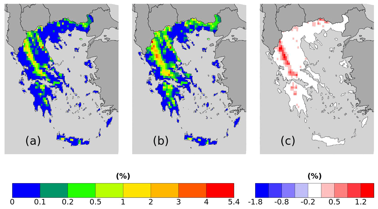
Figure 9 RR20ID ensemble probabilities for (a) empirical and (b) copula method. (c) = (b)–(a).

Both reanalysis products yield greater WCCEs probabilities in the Pindus mountains, although due to its finer spatial resolution, WRF_ERA_I display high probabilities at other mountainous regions located in Crete, Peloponnese, Evia Island, and others. Also, in both WCCEs copula method yields higher probabilities, especially for WRF_ERA_I and the RR20FD case. Moreover, WRF_ERA_I displays a greater range than ERA5 with RR20FD probabilities reaching 13.83 % and RR20ID 10.48 % compared to 1.83 % and 0.55 % of ERA5 respectively (Figs. 6 and 7).

4.2 Projections ensemble

Figures 8 and 9 yield that the ensemble mean displays similar to the WRF_ERA_I spatial distributions of WCCEs. RR20FD and RR20ID probabilities reach 10.8 % and 5.4 % respectively. The copula method yields higher probabilities for both methods in mountainous regions with greater differences displayed for RR20ID events in the Pindos mountain range and RR20FD exhibiting greater spatial distribution in differences between the two methods.

Table 6 Table exhibiting mean (MEAN) RR20ID empirical probabilities station probabilities (%) for observations and models, standard deviation (SD), bias (BIAS), rmse (RMSE), Pearson correlation (COR), and CSI of models against observations.

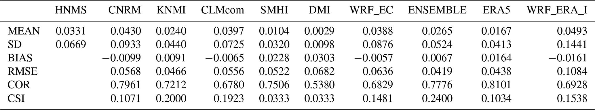
Table 7 Table exhibiting mean (MEAN) RR20ID copula probabilities station probabilities (%) for observations and models, standard deviation (SD), bias (BIAS), rmse (RMSE), Pearson correlation (COR), and CSI of models against observations.

5 Past–future ensemble differences

This section displays the differences of the ensemble mean WCCEs probabilities, calculated for the empirical and the copula method, compared to the past probabilities presented in the previous section. The differences mapped are statistically significant at a 95 % level using the student's t test (Goulden, 1939) comparing 25 annual values of the time series.

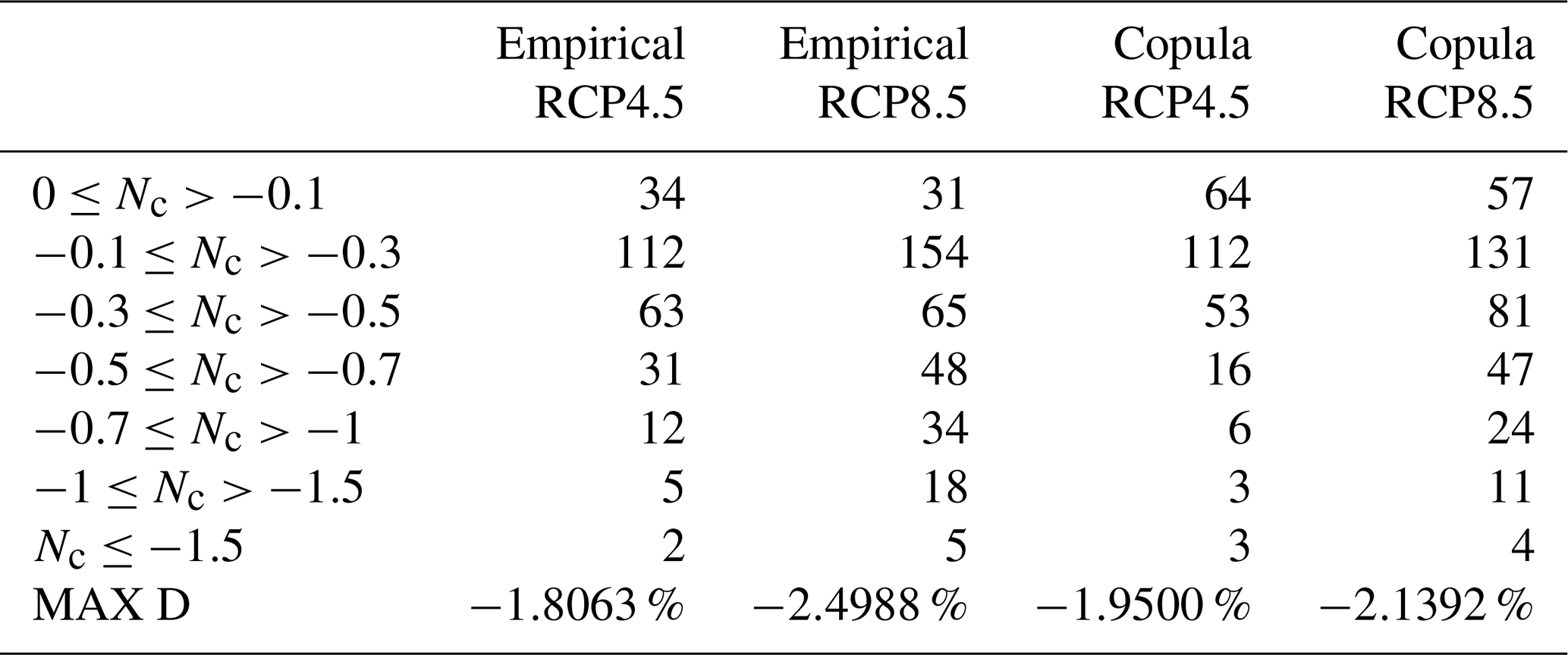
5.1 RR20FD

From the results displayed in Figs. 10 and 11 and in Table 8, RCP4.5 and RCP8.5 scenarios for the probabilities of the RR20FD events, we observe that in all cases future scenarios yield only negative values, meaning the reduction of RR20FD events in the 2025–2049 period compared to 1980–2004 period in all mountainous regions of Greece. RCP8.5 yields a greater reduction of RR20FD probabilities than the RCP4.5 scenario both in spatial distribution and extreme values. The empirical method exhibits a greater reduction for the RCP8.5 scenario, although for the RCP4.5 scenario both methods yield similar results.

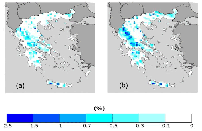
Figure 10 RR20FD empirical method probability differences of future–past periods for (a) RCP4.5 and (b) RCP8.5 scenarios.

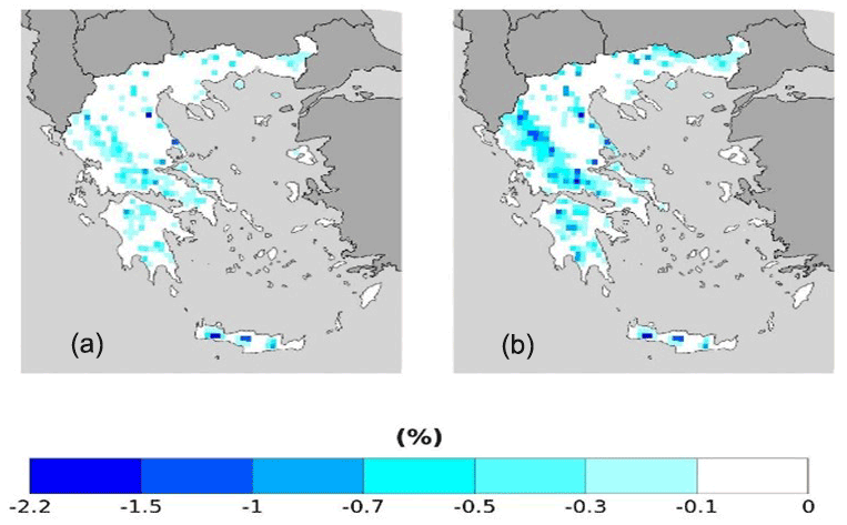
Figure 11 RR20FD copula method probability differences of future–past periods for (a) RCP4.5 and (b) RCP8.5 scenarios.

Table 8 Ensemble number of cells (N_c) in each category of probability difference (%) for RR20FD for empirical and copula method. MAX D denotes the maximum negative difference between future and past periods. N_v concerns only cells with statistically significant difference.

5.2 RR20ID

Similarly to RR20FD, RR20ID events probabilities yield only zero or negative differences compared to the past for both scenarios (Figs. 12 and 13). Empirical and copula methods yield similar results in distribution and extreme values. For both methods, the RCP4.5 scenario tends to higher reduction of RR20ID probabilities than RCP8.5, as observed in Table 9.

Table 9 Ensemble number of cells (N_c) in each category of probability difference (%) for RR20ID for empirical and copula method. MAX D denotes the maximum negative difference between future and past periods. N_v concerns only cells with statistically significant difference.

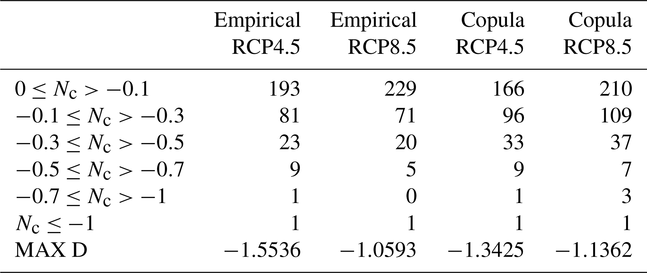
The results for both scenarios and events show that independently from the choice of scenario, the probabilities of the events are expected to reduce almost equally in the near future (2025–2049) compared to the past period (1980–2004).

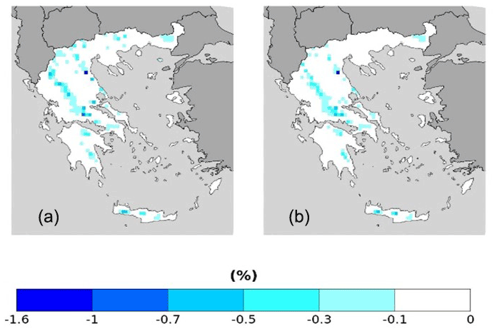
Figure 12 RR20ID empirical method probability differences of future–past periods for (a) RCP4.5 and (b) RCP8.5 scenarios.

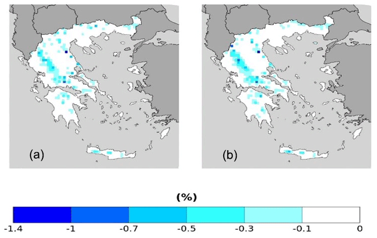
Figure 13 RR20ID copula method probability differences of future–past periods for (a) RCP4.5 and (b) RCP8.5 scenarios.

6 Discussion and conclusions

This work presents for the first time to our knowledge an extensive study of wet–cold compound events in Greece for the historical and future periods of 1980–2004 and 2025–2049, respectively. Models' data from the EURO-CORDEX initiative of 0.11^∘ resolution and reanalysis data (ERA5 and ERA-Interim dynamically downscaled to 5 km²) were used and validated for the determined WCCEs against the formally available observational datasets by HNMS for the country. The number of events and their probabilities of occurrence were determined by applying a fixed thresholds approach. Then, the bivariate validation of the models' datasets against observations was performed for the determined bivariate thresholds. The probabilities of WCCEs were computed using the empirical method and the best-fitted copula for the bivariate time series for observational data, reanalysis, projection models, and the ensemble of the projection models. Copulas yield higher extreme events probabilities for most of the cases considering the dependence between temperature and precipitation.

Although uncertainties may rise on the impact of WCCEs on mountainous areas due to the absence of observations on altitudes higher than 1000 m, we trust the results yielded by the ensemble. Besides the satisfying results from the bivariate validation, this trust is enhanced by the fact that winter period systems affect large areas crossing the country from north to south or from west to east (Cartalis et al., 2010), and therefore recorded by available stations. Also, in the cold period of the year, convective precipitation forced by orography is limited, hence the doubt that the models do not simulate extreme rainfall in winter is reduced. Moreover, the use of the ensemble mean of the models reduces the uncertainties in models' ability to simulate the probability of the occurrence of extreme events. The reduction of RR20FD and RR20ID WCCEs on mountains that the ensemble of projection models predict in the future might contribute to less heavy snowfall events and possibly less accumulated snow depth. If such a scenario will be verified, Greece faces the threat of losing the main sources of fresh water that come from melted mountain snow during spring or early summer in the near future period. The rise of temperature due to global warming is the main factor for the reduction of WCCEs (Figs. S5–S7), while also possible changes in patterns of teleconnections may affect winter conditions in Greek mountains, similar to NAO (North Atlantic Oscillation) pattern affecting Pindos mountains (López-Moreno et al., 2011) or the positive phase of EAWR (East Atlantic–Western Russia) pattern that leads to cold air advection from the north towards the southern part of Europe and the eastern Mediterranean region (Ionita, 2014). Still, understanding extreme events on complex terrains demands greater effort from the scientific community to enable solid predictions on the impact of climate change on the occurrence of these events.

Appendix A

Table A1 HNMS stations information.