the Creative Commons Attribution 4.0 License.
the Creative Commons Attribution 4.0 License.
 | 27 Sep 2022
Trends and uncertainties of mass-driven sea-level change in the satellite altimetry era
Carolina M. L. Camargo
Riccardo E. M. Riva
Tim H. J. Hermans
Aimée B. A. Slangen
Ocean mass change is one of the main drivers of present-day sea-level change (SLC). Also known as barystatic SLC, ocean mass change is caused by the exchange of freshwater between the land and the ocean, such as melting of continental ice from glaciers and ice sheets, and variations in land water storage. While many studies have quantified the present-day barystatic contribution to global mean SLC, fewer works have looked into regional changes. This study provides an analysis of regional patterns of contemporary mass redistribution associated with barystatic SLC since 1993 (the satellite altimetry era), with a focus on the uncertainty budget. We consider three types of uncertainties: intrinsic (the uncertainty from the data/model itself), temporal (related to the temporal variability in the time series) and spatial–structural (related to the spatial distribution of the mass change sources). Regional patterns (fingerprints) of barystatic SLC are computed from a range of estimates of the individual freshwater sources and used to analyze the different types of uncertainty. Combining all contributions, we find that regional sea-level trends range from −0.4 to 3.3 mm yr−1 for 2003–2016 and from −0.3 to 2.6 mm yr−1 for 1993–2016, considering the 5–95th percentile range across all grid points and depending on the choice of dataset. When all types of uncertainties from all contributions are combined, the total barystatic uncertainties regionally range from 0.6 to 1.3 mm yr−1 for 2003–2016 and from 0.4 to 0.8 mm yr−1 for 1993–2016, also depending on the dataset choice. We find that the temporal uncertainty dominates the budget, responsible on average for 65 % of the total uncertainty, followed by the spatial–structural and intrinsic uncertainties, which contribute on average 16 % and 18 %, respectively. The main source of uncertainty is the temporal uncertainty from the land water storage contribution, which is responsible for 35 %–60 % of the total uncertainty, depending on the region of interest. Another important contribution comes from the spatial–structural uncertainty from Antarctica and land water storage, which shows that different locations of mass change can lead to trend deviations larger than 20 %. As the barystatic SLC contribution and its uncertainty vary significantly from region to region, better insights into regional SLC are important for local management and adaptation planning.
- Article
(13408 KB) - Full-text XML
- BibTeX
- EndNote


Even if all countries respect the Paris Agreement, global mean sea level will continue to rise in the coming decades and beyond (Wigley, 2005; Nicholls et al., 2007; Oppenheimer et al., 2019; Fox-Kemper et al., 2021). The reason for this is the long response time of the ocean and the cryosphere to climate change (Abram et al., 2019). As a consequence, coastal societies all over the world will need to deal with a certain amount of sea-level change (SLC). Therefore, a good understanding of present-day SLC and its drivers is required, as it yields better future sea-level projections, which are necessary for adaption and mitigation planning.
The attribution of SLC to its different drivers is known as the sea-level budget (WCRP, 2018). Alongside density-driven (steric) changes (e.g., MacIntosh et al., 2017; Camargo et al., 2020), present-day SLC is mainly driven by the mass loss of continental ice stored in glaciers and ice sheets and by variations in land water storage (LWS) (WCRP, 2018; Fox-Kemper et al., 2021). The contribution of ocean mass changes, termed barystatic SLC (Gregory et al., 2019), was responsible for about 60 % of the global mean SLC over the 20th century (Frederikse et al., 2020; Fox-Kemper et al., 2021). Barystatic SLC varies significantly from region to region and strongly depends on the location of terrestrial mass loss (Mitrovica et al., 2001). For example, a collapse of the West Antarctic Ice Sheet would cause sea level to rise 1.6 times more in San Francisco (US) than in Santiago (Chile) (Gomez et al., 2010). Thus, for local management and climate planning, it is important to understand the barystatic contribution to regional SLC (Larour et al., 2017).
The regional patterns associated with barystatic SLC can be computed by solving the sea-level equation (SLE) (Farrell and Clark, 1976), which results in the so-called sea-level fingerprints (Mitrovica et al., 2001). These patterns reflect the so-called gravitational, rotational and deformation (GRD) response of the Earth to mass redistribution (Gregory et al., 2019). GRD-induced sea-level fingerprints have been the subject of several studies, ranging in scope from paleoclimatic SLC, for example due to the last deglaciation event (Lin et al., 2021), to contemporary SLC (Frederikse et al., 2020) and future sea-level projections (e.g., Slangen et al., 2012, 2014). Most of the studies including present-day mass contributions have focused either on the GRACE satellite period (since 2002) (Bamber and Riva, 2010; Riva et al., 2010; Hsu and Velicogna, 2017; Adhikari et al., 2019; Frederikse et al., 2019), on the closure of the sea-level budget over a longer period (Slangen et al., 2014; Frederikse et al., 2020) or on their contribution to global mean SLC (Chambers et al., 2007; Horwath et al., 2021). However, an in-depth analysis of the GRD-induced regional patterns associated with barystatic SLC and its uncertainties during the satellite altimetry era (since 1993) has not yet been done. Insights into the contemporary contributions of ice sheets, glaciers and land water storage to regional SLC and their uncertainties over the last 3 decades are important to constrain regional sea-level projections and obtain a better closure of the regional sea-level budget.
The importance of quantifying the uncertainties in sea-level studies has increasingly received attention (Bos et al., 2014; Royston et al., 2018; Ablain et al., 2019; Camargo et al., 2020; Palmer et al., 2021; Prandi et al., 2021; Horwath et al., 2021). One of the approaches to describe the uncertainties of a system is to partition the total uncertainty budget into different kinds of uncertainties. Errors in the measurement system, known as intrinsic uncertainties (Palmer et al., 2021), describe the sensitivities of choices within a methodology (Thorne, 2021). The intrinsic uncertainties, also referred to as observational (Ablain et al., 2019; Prandi et al., 2021) or parametric (Thorne, 2021), need to be determined during the low-level data processing and are usually provided with higher-level (ready-to-use) products. Another class of uncertainties originates from the use of different methodologies to describe the same physical system, known as structural uncertainty (Thorne et al., 2005; Palmer et al., 2021). This can be defined as the spread around a central (ensemble) estimate. The structural uncertainty is related to the use of different datasets of the same process. Note that, if different datasets use the same product for corrections, calibrations and/or validation, the intrinsic and structural uncertainties could be partially correlated. Regarding the GRD-induced pattern associated with barystatic SLC, the spread in the location of the mass change introduces another source of error, which we call spatial uncertainty. Finally, another type of uncertainty results from the autocorrelation of the observations (Bos et al., 2013), which we refer to as temporal uncertainty. This uncertainty becomes relevant when a functional model, such as a (linear) trend, is used to describe the changes within the system. The temporal uncertainty can be estimated by using noise models while determining the trend. Together, the intrinsic, structural, spatial and temporal uncertainties describe the uncertainties of an observed quantity, in this case the GRD-induced pattern associated with barystatic SLC.
The aim of this work is to provide a comprehensive overview of barystatic SLC and the associated regional GRD-induced patterns with a focus on the global and regional uncertainty budget. Throughout this paper, we use “GRD-induced SLC” when referring to the GRD-induced regional pattern associated with barystatic SLC. We use state-of-the-art datasets of mass contributions from land ice and LWS (Sect. 2.1) to compute regional sea-level fingerprints (Sect. 2.2.1). In addition, we present a methodological framework to describe the uncertainties of the fingerprints (Sect. 2.2.2). We follow the noise model analysis of Camargo et al. (2020) to quantify the temporal uncertainty (Sect. 3.1; 3.2). We combine the effect of ice geometry on sea-level fingerprints (Bamber and Riva, 2010; Mitrovica et al., 2011) with the structural uncertainty definition of Palmer et al. (2021) to compute the spatial–structural uncertainty of the fingerprints (Sect. 3.3). Together with the intrinsic uncertainty (Sect. 3.4), we present the total GRD-induced SLC trend and uncertainty for 2003–2016 and 1993–2016 (Sect. 3.5). We finalize this paper with an overview and a discussion of our findings (Sect. 4).
2.1 Datasets
To obtain the GRD-induced SLC patterns we use a range of estimates of mass changes of the Antarctic and Greenland ice sheets (AIS and GIS, respectively), glaciers (GLA), and land water storage (LWS). We define LWS anomalies as water mass changes outside glacierized areas: the sum of water stored in rivers, lakes, wetlands, artificial reservoirs, snow pack, canopy and soil (groundwater) (Cáceres et al., 2020). For each of the contributions we use four different estimates (Table 1, Fig. 1, and discussed in more detail in Supplementary Text A). Despite the methodological differences between the datasets, they show a good agreement in reproducing the global mean barystatic sea-level changes (Fig. 1)
Table 1Overview of datasets used in this paper.
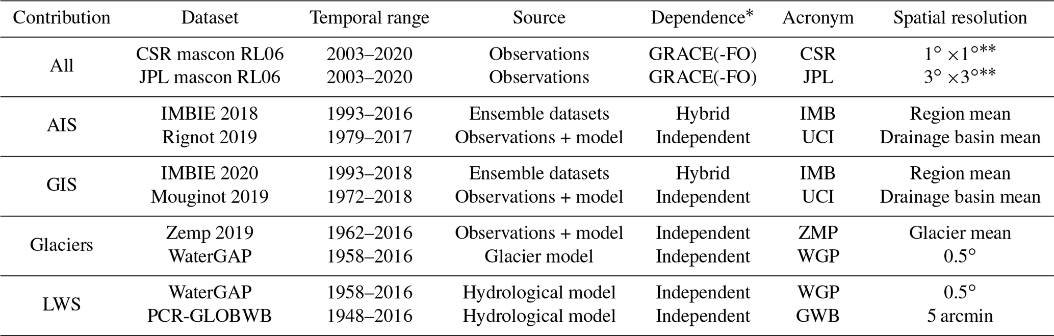
* Dataset dependence on GRACE. Note that while the mascons are provided in 0.25 and 0.5∘ resolution, the native resolutions of the mascon solution are 1∘ and 3∘ equal-area grids at the Equator for CSR and JPL, respectively (Save et al., 2016; Watkins et al., 2015).

Figure 1Global mean barystatic sea-level change time series. Different components are vertically offset for visualization purposes.
One of the main sources of observations of Earth's mass changes is the satellite mission Gravity Recovery and Climate Experiment (GRACE, Tapley et al., 2004) and its follow-on mission (GRACE-FO, Landerer et al., 2020). We use GRACE mass concentrations (mascons) over land as estimates of changes in AIS, GIS, glaciers and LWS. To avoid methodological biases, we use mascon solutions from two different processing centers: RL06 from the Center for Spatial Research (CSR) (Save et al., 2016; Save, 2020) and RL06 v02 from the Jet Propulsion Laboratory (JPL) (Watkins et al., 2015; Wiese et al., 2019) (Table 1). JPL and CSR mascons are provided on a 0.5 and 0.25∘ long–lat grid, respectively, but they actually are resampled from the native 3∘ and 1∘ equal-area grids (Save et al., 2016; Watkins et al., 2015). Considering the native resolution of GRACE observations of about 300 km at the Equator (Tapley et al., 2004), the JPL mascons should have independent solutions at each mascon center, with uncorrelated errors, while the CSR mascons are not fully independent of each other and are expected to contain spatially correlated errors.
To isolate the individual contributions of AIS, GIS, LWS and GLA in the GRACE mascons, we use an ocean–land–cryosphere mask (Supplement Fig. B1), which delineates the drainage basins of the ice sheets (based on Mouginot and Rignot, 2019, Rignot et al., 2011), the glaciers (based on the Randolph Glacier Inventory, Consortium, 2017) and the remaining land regions (based on ETOPO1, Amante and Eakins, 2009). Considering the size of glaciers, the resolution of the GRACE signal is not high enough to (i) separate the peripheral glaciers from the ice sheets and (ii) to separate the signal of glaciers and LWS in regions with small glacier coverage and large LWS contribution. Thus, to isolate the glacier signals from the mascons, we follow the method described in Reager et al. (2016) and Frederikse et al. (2019).
-
Peripheral glaciers to Greenland and Antarctica are included with the ice sheet mass changes.
-
Regions where glaciers dominate the mass changes are considered “full” glaciers; that is, the land signals in those regions are purely denoted as glacier mass change. These include the RGI regions of Alaska, Arctic Canada North, Arctic Canada South, Iceland, Svalbard, Russian Arctic Islands and Southern Andes.
-
For the remaining glaciated regions, we assume that the mass change is partly due to glacier mass change and partly due to LWS (“split” glaciers).
In these regions the glacier mass changes are known to be small, and mass changes are dominated by LWS. We use the glacier estimates of Hugonnet et al. (2021), which are based on satellite and airborne elevation datasets, as our glacier estimates in these regions. Unlike gravimetry observations, the estimates of Hugonnet et al. (2021) do not include the hydrological “contamination”. To isolate the glacier from the LWS signal, we subtract the corrected glacier estimates from the total mass change in the mascons. The remaining signal is then added to the LWS contribution.
Apart from GRACE data, which are only available since late 2002, we use seven other datasets in our analysis, from which five are independent of GRACE and two partly incorporate GRACE information (Table 1). For LWS, we use data from two global hydrological models: PCR-GLOBWB (GWB, Sutanudjaja et al., 2018) and WaterGAP (WGP, Cáceres et al., 2020). The latter also incorporates a time series of glacier mass variations from the global glacier model of Marzeion et al. (2012). We use the ocean–land–cryosphere mask (Supplement Fig. B1) to separate the LWS and GLA estimated from WGP. For GLA, in addition to the WGP model simulations, we also use observational estimates from Zemp et al. (2019), which are based on an extrapolation of glaciological and geodetic observations. For the GIS and AIS, we use observation- and model-based data from Mouginot et al. (2019) and Rignot et al. (2019), respectively. We refer to these as UCI datasets, since they were both developed at the University of California at Irvine (UCI). We also use AIS and GIS estimates from the ice sheet mass balance inter-comparison exercise (IMBIE, Shepherd et al., 2018, 2020), which combines ice sheet mass balance estimates developed from three different techniques (satellite altimetry, satellite gravimetry (GRACE) and the input–output method).
2.2 Methodological framework
We characterize GRD-induced SLC by a linear trend and the three types of uncertainties discussed earlier. We use the following time periods for the trend analysis: from 1993–2016 for the non-GRACE datasets and from 2003–2016 for all datasets. The framework used to compute and combine the uncertainties and associated regional sea-level patterns is schematized in Fig. 2. The main modules of the framework (bold text in the blue boxes of Fig. 2a) are further explained in Fig. 2b and in Sects. 2.2.1 and 2.2.2.
The trends and associated temporal uncertainties are estimated directly from the mass source time series (Table 1) in the noise model module (Fig. 2a). Thus the noise model analysis (Sect. 3.1) describes the physical processes of the mass sources instead of the temporal correlation in the sea-level fingerprint. The mass source change trend and temporal uncertainty are then used as input to the SLE model module (Sect. 2.2.1), which computes how the mass changes on land affect regional ocean mass change (i.e., GRD-induced SLC; Sect. 3.2). The mass source trends are also used as input to the spatial uncertainty analysis (Sect. 3.3). The uncertainty of the mass source time series is used as input to the intrinsic uncertainty analysis (Sect. 3.4).
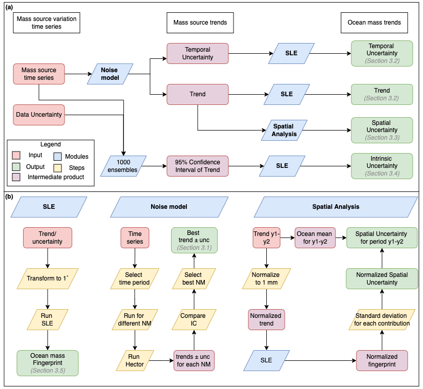
Figure 2Overview of the framework used in this study (a), with detailed modules (b). Red boxes indicate the initial data (Table 1), purple the intermediate products and green the final products. The yellow boxes indicate steps of the methodology and the blue the main modules. We use the following acronyms and abbreviations: OLS: ordinary least squares; SLE: sea-level equation; IC: information criteria; unc: uncertainty; NM: noise model; Hector: software package by Bos et al. (2013).
2.2.1 The sea-level equation model
The regional GRD-induced SLC patterns resulting from the barystatic contributions can be computed by solving the sea-level equation (SLE) (Farrell and Clark, 1976), using spatial and temporal information of GLA, AIS, GIS and LWS (Mitrovica et al., 2001; Tamisiea and Mitrovica, 2011). Before computing the regional SLC fields, all input data (Table 1) are converted to equivalent water height and bilinearly interpolated to a 1∘ by 1∘ grid. The SLE model then computes how the source mass change is redistributed over the oceans, taking into account the GRD response of the Earth to these mass changes (Milne and Mitrovica, 1998; Mitrovica et al., 2001; Tamisiea and Mitrovica, 2011). The SLE model uses a pseudospectral approach (Mitrovica and Peltier, 1991) up to spherical harmonic degree and order 180 (equivalent to a spatial resolution of 1∘). We assume a purely elastic solid-Earth response to the mass redistribution, based on the Preliminary Reference Earth Model (Dziewonski and Anderson, 1981). While we focus here on the fingerprints of relative SLC, that is, the difference in height between the geoid and the solid Earth surface, we also provide the complementary geocentric (absolute) fingerprints (see the Data availability section).
2.2.2 Trend and uncertainty assessment
Our GRD-induced SLC and associated temporal uncertainty (Fig. 2, center column) are computed using the software package Hector (Bos et al., 2013), in which the observations are assumed to be the sum of a deterministic model (including annual and semi-annual signals) and stochastic noise. Different noise models can be selected to describe the autocorrelation between the residuals of the regression. The uncertainty of the regression model, representing 1 standard deviation, is then used as our temporal uncertainty.
Based on previous studies (Bos et al., 2013; Royston et al., 2018; Camargo et al., 2020), we test eight noise models to find the best descriptor of the uncertainties in our data:
-
white noise (WN), in which no autocorrelation between the residuals is considered;
-
pure power law (PL), where all observations influence one another, although their correlation decreases with increasing temporal distance;
-
PL combined with WN (PLWN);
-
auto-regressive of orders 1, 5 and 9 (AR(1), AR(5) and AR(9), respectively), in which the order represents the number of previous observations influencing the next one;
-
autoregressive fractionally integrated moving average of order 1 (ARF), which combines an AR(1) model with a fractional integration and a moving average of the noise;
-
generalized Gauss–Markov (GGM), a generalized form of the ARF model.
The goodness of the fit of the models is assessed with the modified Bayesian information criterion (BICtp; He et al., 2019), which is an intermediate criterion in relation to the Akaike (AIC; Akaike, 1974) and Bayesian (BIC; Schwarz, 1978) criteria. The best noise model is the one that minimizes these criteria. Since these criteria are relative values, they can not be compared between different datasets. Thus, we compare the criteria of different noise models for each dataset and each grid point separately. To select the best noise model, we compute the relative likelihood of the BICtp and select the model with values smaller than 2 (Burnham and Anderson, 2002; Camargo et al., 2020). Note that all noise models reasonably capture the variability of the time series (Fig. B2), as their scores are always within a similar range.
The second uncertainty we consider is the spatial–structural uncertainty (Fig. 1b, right column). Studies that combine a large number of datasets often base the structural uncertainty of an estimate on the standard deviation over the individual datasets in relation to the ensemble mean (Palmer et al., 2021). To isolate the effect that the spatial distribution of the terrestrial mass change has on the fingerprints, we compute the spatial–structural uncertainty by estimating the standard deviation for each contribution based on normalized fingerprints. The latter means that the sum of the regional SLC for each contribution is equal to 1 mm yr−1 of SLC. By using normalized fingerprints we remove the weight that the different central estimates (mean) have on the spatial standard deviation. We then take the standard deviation across the four normalized datasets for each mass source contribution, obtaining four normalized spatial–structural uncertainties, which reflects the uncertainty associated with the different spatial resolutions and location of mass change of the datasets. For example, the spatial–structural uncertainty of the AIS reflects the differences in the fingerprints due to the fact that GRACE datasets provide observations at a 0.25 ∘ resolution, while UCI provides mass changes averaged over the 17 main drainage basins of the ice sheet and IMBIE mass changes averaged over three regions of the ice sheet (west, east and peninsula). While the analysis is based on the 2003–2016 trend, we assume that the normalized fingerprints are time-invariant and that the resulting uncertainty is also representative of the 1993–2016 period. Lastly, we multiply the normalized uncertainty by the ocean mean (central estimate) of each contribution for 1993–2016 and 2003–2016 to compute the spatial–structural uncertainty for the respective period. We note that all components show some decadal variability in the spatial distribution, and thus assuming that the spatial mass change distributions from 2003–2016 are representative of the period 1993–2016 is an approximation of the study. However, by multiplying the normalized fingerprint by the mean of each period, the possible error from this assumption becomes fairly limited. Furthermore, using a shorter spatially dense time series to obtain the variability of a longer period when only limited information is available is a methodology that is often used in sea-level studies (e.g., Church and White, 2006; Frederikse et al., 2020).
The final type of uncertainty considered in our assessment is the intrinsic uncertainty, which represents the formal errors and sensitivities in the measurement system and needs to be provided with the observations/models by the data processor/distribution center. The intrinsic uncertainty was only provided with the JPL and IMBIE datasets. For all other datasets, our uncertainty budget does not include the intrinsic uncertainty. The uncertainties provided with the JPL mascons represent the scaling and leakage errors from the mascon approach (Wiese et al., 2016) and, over land, are scaled to roughly match the formal GRACE uncertainty of Wahr et al. (2006). The latter represent errors in monthly GRACE gravity solutions, encompassing measurement, processing and aliasing errors (Wahr et al., 2006). While the mascons have been corrected for mass changes due to glacial isostatic adjustment (GIA) with the ICE6G-D model (Peltier et al., 2018), the intrinsic uncertainties of the JPL mascons do not represent the uncertainties from the GIA correction, which can be large depending on the region (Reager et al., 2016; Wouters et al., 2019). For example, the choice of the GIA model used for the correction could lead to uncertainties representing up to 19 % of the signal in Antarctica, but less than 1 % in Greenland (Blazquez et al., 2018). Given that estimating GIA uncertainties is in itself an open issue (Caron et al., 2018; Simon and Riva, 2020), we could not propagate full GIA uncertainties into the fingerprints. Since the intrinsic uncertainty represents systematic errors and instrumental noise, which might be serially correlated, we assume that the errors can be approximated by a random walk. We therefore generate an ensemble of 1000 time series by perturbing the original rate with random normal noise multiplied by the uncertainty time series. We then compute the trend for each ensemble member. We use half of the width of the 95 % CI as input in the SLE model to show how the mass associated with the intrinsic uncertainty is distributed over the oceans.
2.2.3 Combining trends and uncertainties
To compute total GRD-induced SLC trends and their uncertainties, we sum the individual contributions (AIS, GIS, LWS and GLA) as follows, with a total of six combinations: 1. CSR (all), 2. JPL (all), 3. IMB (AIS/GIS) + WGP (LWS/GLA), 4. UCI (AIS/GIS) + WGP (LWS/GLA), 5. IMB (AIS/GIS) + GWB (LWS) + ZMP (GLA) and 6. UCI (AIS/GIS) + GWB (LWS) + ZMP (GLA).
Whereas the trends are added together linearly, we add the uncertainties in quadrature, assuming they are independent and normally distributed. We acknowledge that this is an important assumption, as it is possible that the intrinsic uncertainty will be reflected in the temporal and structural uncertainties. However, we keep the independence assumption to obtain a more realistic (and smaller) estimate of the final uncertainty (Taylor, 1997). For each contribution, we first combine the different types of uncertainty following Eq. (1):
where σCONTR is the total uncertainty for each individual contribution (AIS, GIS, GLA, LWS). We then compute the total GRD-induced uncertainty for all contributions (σtotal) following Eq. (2):
In this section we first present the noise model selection (Sect. 3.1) used to compute the GRD-induced SLC trend and temporal uncertainty (Sect. 3.2). We then present the spatial–structural (Sect. 3.3) and intrinsic uncertainties (Sect. 3.4). Lastly, we show the total GRD-induced SLC trends (i.e., the sum of the different contributions) and uncertainties (i.e., the sum of the different contributions and types of uncertainties) and zoom in on a few coastal examples (Sect. 3.5).
3.1 Noise characteristics of the mass sources
Many geophysical time series are known to exhibit temporal (auto)correlations, as is the case for sea-level and cryosphere data (Bos et al., 2013). This autocorrelation means that each observation is not completely independent from the previous one (Bos et al., 2013), and it is defined by the shape of the spectrum of the time series (Hughes and Williams, 2010). Understanding the shape of spectra and determining the best stochastic model to describe these spectra is important to understand the physics of the processes playing a role in the time series (Hughes and Williams, 2010). In addition, accounting for the autocorrelation of the time series while estimating a linear trend is important both for the value of the trend itself and for the statistical error of the fit (Bos et al., 2013; Hughes and Williams, 2010). Depending on the nature of the process being studied, different noise models can be used to account for the effects of autocorrelations. Here, we determine the best noise model for each spatial data point of the mass sources of the different barystatic contributions (AIS, GIS, LWS, GLA). Our analysis shows that the optimal noise model depends on both the physical system (AIS, GIS, GLA or LWS) and the dataset (Fig. 3).
There are clear differences between the GRACE datasets (Fig. 3a–h), for which the PL and GGM noise models score higher, and the other datasets (Fig. 3i–p), for which the AR(5) and AR(9) models score higher. The only exception is for the two Greenland datasets (GIS_JPL (f) and GIS_IMB (j)), where the noise model selection is reversed. Over the ice sheets, the higher resolution of GRACE observations (compared to IMBIE and UCI datasets) leads to more heterogeneity in the model selection, which suggests the inclusion/capture of more complex processes. For example, our analysis indicates that only one type of noise model is selected for the entire ice sheet in the IMBIE dataset (Fig. 3i–j). For LWS changes, where the spatial resolution of GRACE and the hydrological models is relatively high, the noise model selection follows a different pattern. There is a general preference for AR(1) in areas with smaller LWS changes (i.e., not the large drainage basins). On the other hand, over the large drainage basins, the same model preference mentioned above is maintained (Fig. 3, right column). This suggests that GRACE observations and the hydrological models might not always be capturing the same processes.
Different noise models are selected as optimal for the two GRACE datasets: CSR datasets (Fig. 3a–d) are best explained with the PL model, while JPL estimates (Fig. 3e–h) are best explained with the GGM model. However, the GGM model is fairly similar to a pure power-law model under certain parameters. Furthermore, the noise model selection for the CSR dataset over the ice sheets (Fig. 3a, b) displays an interesting pattern, which is not seen for the JPL dataset (Fig. 3e, f). Regions with relatively strong ice melt (i.e., the Antarctica Peninsula, East Antarctica and northwest of Greenland) are better represented by an AR(5) model. Over the extremities of the ice sheets, which are more dynamic regions, the GGM model is the optimal one. On the other hand, internal regions of the ice sheets, where there is little ablation, are better described by the PL model.

Figure 3Noise model selection based on the time series of the different sources of mass loss for each dataset (rows) and contribution (columns), over the period 2003–2016.
3.2 Trend and temporal uncertainty
The mass source trend and uncertainties obtained with the selected noise models (Sect. 3.1) are used to compute the sea-level fingerprints (Fig. 4). To illustrate the difference between the fingerprints based on GRACE and those based on GRACE-independent datasets, we show the trends and uncertainties for the JPL estimates (Fig. 4a–d, i–l) and for the UCI estimates for the ice sheets (Fig. 4e–h) and WaterGAP for glaciers and LWS (Fig. 4m–p). Trends and temporal uncertainties for the other datasets are provided in Fig. B3. The typical GRD patterns are visible in all fingerprints: regions closer to a freshwater source experience a negative SLC, due to the mass loss that causes land uplift and reduced gravitational attraction, while in the far field the sea level rises more than the global average.
While all trends strongly depend on the dataset (Fig. 4, first and third columns), the uncertainty patterns are rather consistent. This suggests that, even though different noise models were used to compute the trend for each dataset, the temporal uncertainty is characteristic of each contribution. We find that for any given contribution, the trends from different datasets are consistent within their respective uncertainties. For glaciers and the ice sheets, the GRACE-independent datasets give a higher trend than the GRACE observations. The temporal uncertainties for ice sheets and glaciers are relatively small, especially for the UCI datasets. This indicates that these contributions do not exhibit strong autocorrelations, and consequently the uncertainty of the trend will be small. On the other hand, the temporal uncertainty for the LWS is larger than the trend itself, and therefore the LWS trend is not statistically significant. This is probably related to the large internal and decadal variability of the time series, in combination with the relatively short period under study.
The largest inter-dataset differences are displayed in the regional patterns of the LWS contribution. Despite the similar global mean LWS trend value for both JPL and WGP, the regional trend patterns and uncertainty values are very different. This may partially be related to the coarse resolution of GRACE (300 km) in comparison to the hydrological models (0.5∘ by 0.5∘ grid; 55 km by 55 km at the Equator). This difference can also be related to the difficulty in modeling the complex processes affecting LWS, which relies on parameterizations of physical processes and on sparse observations, while GRACE measures the total mass change.
Another significant inter-dataset difference is in the regional trend pattern as a consequence of AIS mass change (Fig. 4a, e). This is mainly related to the location of ice mass changes in each dataset. GRACE observes mass accumulation in East Antarctica, resulting in a positive sea-level trend in the region. This accumulation is not captured by the UCI and IMB datasets. GRACE has a higher spatial resolution, and thus provides more detail of where the mass change is taking place. The UCI dataset provides estimates on a basin scale, so more detailed changes may be averaged out. The effect of the location of mass change at the source of the contribution is further investigated with the spatial–structural uncertainty (next section).
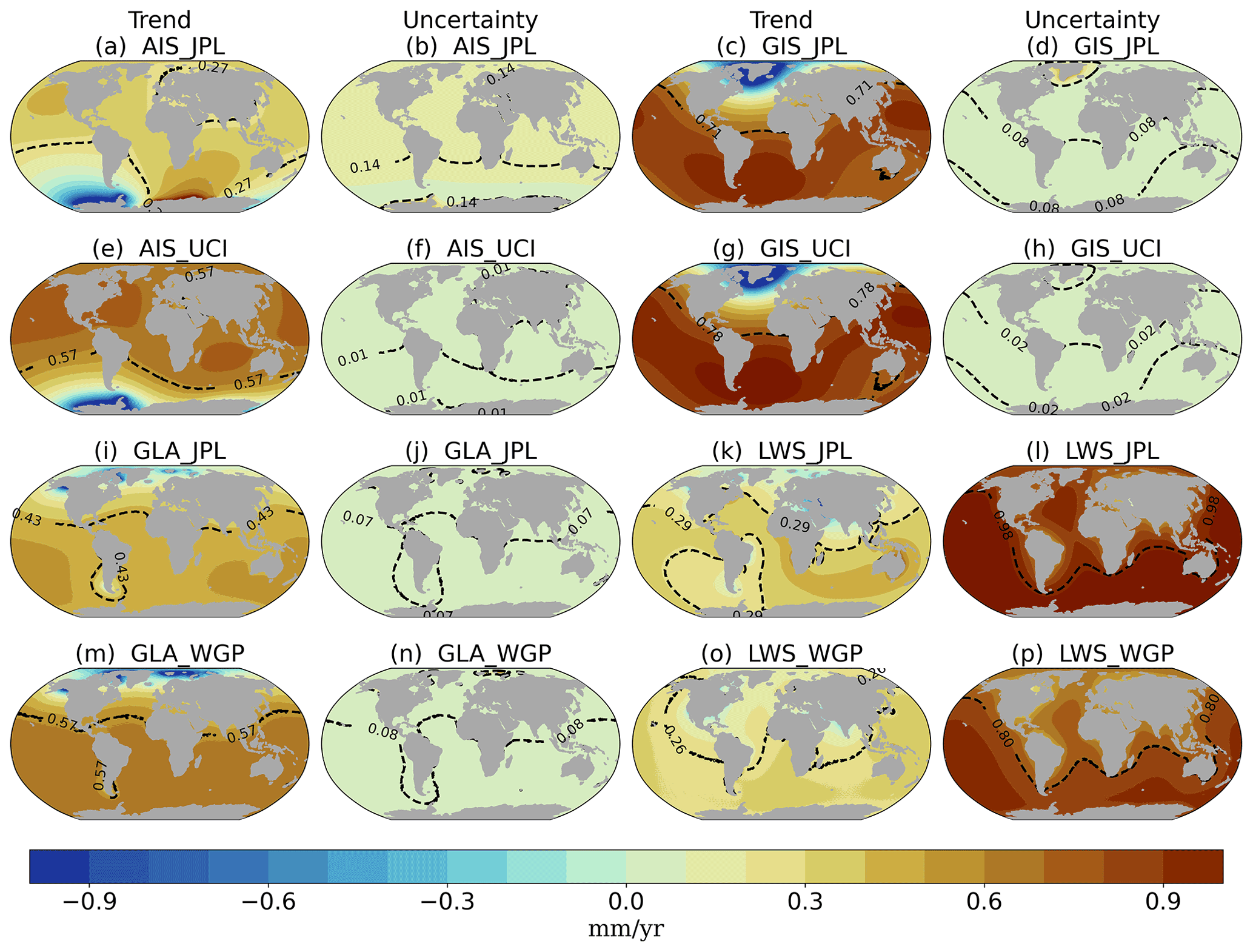
Figure 4GRD-induced sea-level trend and temporal uncertainty (mm yr−1) for GRACE (JPL) and independent combination (UCI + WGP) for 2003–2016. The black dashed contour line and number indicate the spatial average of the regional trend and uncertainty. Trends and uncertainties of CSR, IMB, ZMP and GWB presented in Supplement Fig. B3.
3.3 Spatial–structural uncertainty
The regional SLC fingerprints directly reflect the differences in the spatial distribution of the mass change sources of the datasets (Mitrovica et al., 2011). Over the ice sheets, for instance, IMBIE provides one time series for the entire Greenland Ice Sheet, which is subdivided into dynamic and surface mass balance changes, and the Antarctic Ice Sheet is divided into three drainage basins. GRACE products, on the other hand, have a native resolution of about 300 km at the Equator (Tapley et al., 2004). To account for the uncertainties arising from the differences in location of the mass change between datasets, we first normalize the fingerprints and then combine them into estimates of the spatial–structural uncertainty (Fig. 5).
For all contributions, the largest spatial uncertainties are concentrated closer to the mass change sources, while the uncertainties are reduced in the far field. The effect of differences resulting from Earth rotational effects (typically leading to four large quadrants) is visible in the far field of the AIS (in the North Pacific) and near hotspots of LWS (around the Southern Ocean). As was the case for the trends (Fig. 4a), the AIS shows the strongest spatial differences, as the underlying datasets strongly differ in their spatial detail. The spatial uncertainties represent the error introduced by using datasets that have insufficient resolution to solve the processes being analyzed. In addition, it also shows that different physical processes are captured by the different datasets, as is the case for the LWS estimate. The discrepancies between the processes captured by GRACE and LWS models result in the spatial–structural uncertainty of the LWS component (Fig. 4d) being the second largest.
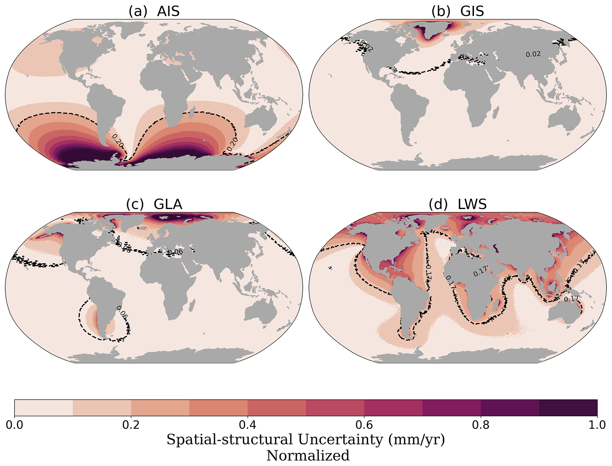
Figure 5Normalized GRD-induced sea-level change fields of the spatial–structural uncertainty (0–1 mm yr−1), representing the uncertainty arising from the different locations of mass changes for Antarctica (a), Greenland (b), glaciers (c) and land water storage (d). The black dashed contour line and number indicate the spatial average of the regional uncertainty.
3.4 Intrinsic uncertainty
The final type of uncertainty considered here is the intrinsic uncertainty, which represents noise related to the dataset itself (Fig. 6). With the exception of the LWS, all intrinsic uncertainties are relatively small (spatial averages below 0.1 mm yr−1). The largest intrinsic uncertainty is seen in the LWS contribution (Fig. 6a), with maximum values of 0.5 mm yr−1. This is expected, as the uncertainty of GRACE is estimated from the standard deviation of the signal anomalies (Wahr et al., 2006), which may lead to an overestimation of the uncertainty in regions where the anomalies represent real hydrological signals (Humphrey and Gudmundsson, 2019). Furthermore, GRACE mass errors are latitude dependent, increasing from the poles to the Equator (Wahr et al., 2006), which explains why we see large intrinsic uncertainty for LWS and low values for the ice sheets and glaciers. The IMBIE datasets (Fig. 6e, f) show larger intrinsic uncertainty than the ice sheet uncertainties from JPL (Fig. 6c, d), once the IMBIE time series is an ensemble of several datasets and methods. Note that these uncertainties are smaller than those originally reported in the IMBIE studies (Shepherd et al., 2018, 2020), which include not only intrinsic but also structural and temporal uncertainties. Overall, the intrinsic uncertainty, which depends on the method employed to produce the estimates, is small compared to the spatial–structural and temporal uncertainties, which are related to the physical processes represented.
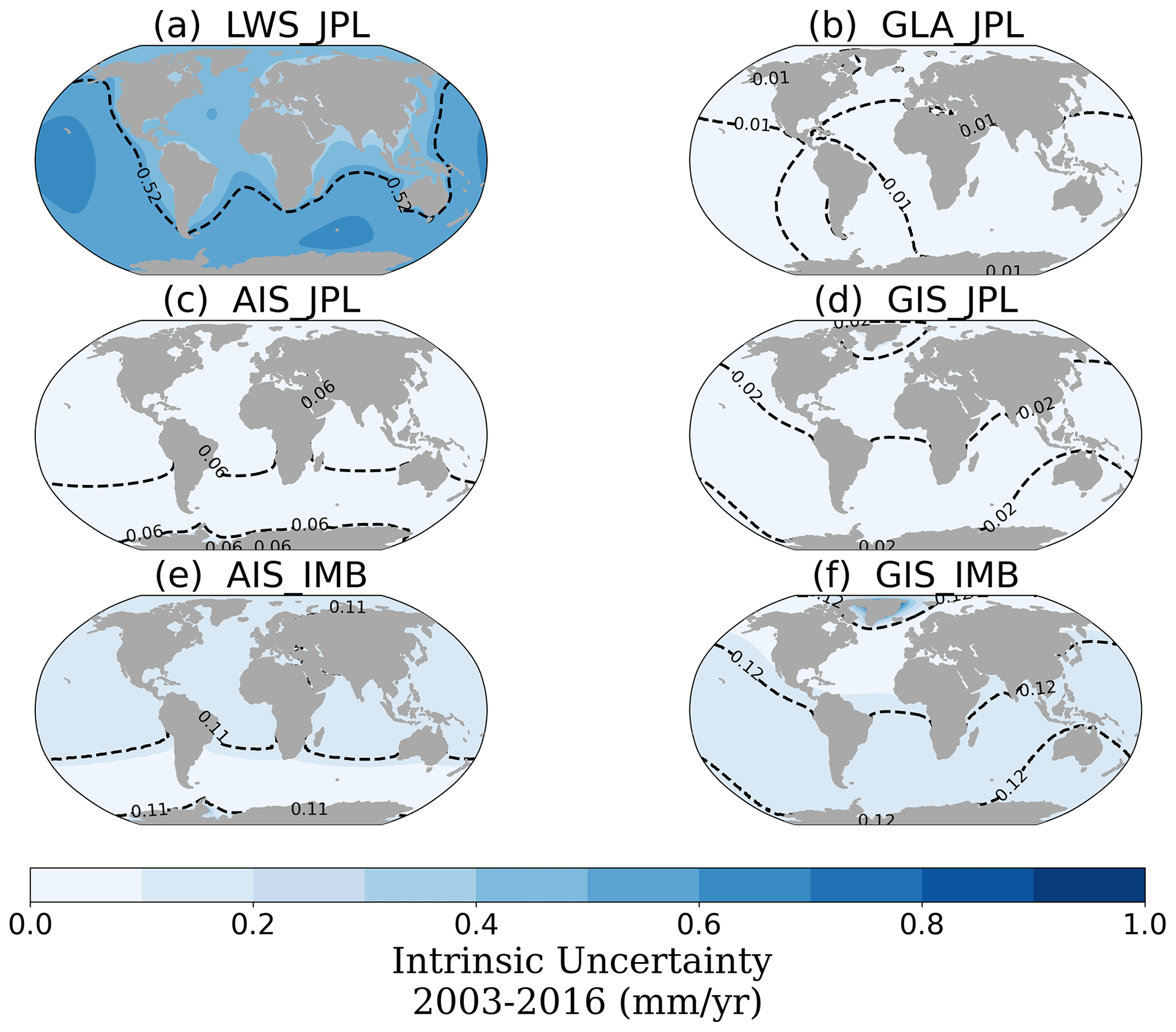
Figure 6GRD-induced sea-level fields of the intrinsic uncertainty (mm yr−1) for the land water storage (a), glaciers (b), Antarctica (c) and Greenland (d) contributions of the JPL dataset and Antarctica (e) and Greenland (f) contributions of the IMBIE dataset. The black dashed contour line indicates the spatial average of the regional uncertainty
3.5 Total barystatic trend and uncertainty
Combining the different contributions, as explained in Sect. 2.2.3, leads to the total GRD-induced SLC trends and uncertainties shown in Fig. 7. Although we analyzed six dataset combinations, here we show only two (JPL and IMB+WGP) to discuss the patterns and the total uncertainty fields. We show these specific combinations because they present the most complete uncertainty budget (as only JPL and IMB provided intrinsic uncertainties). Additional combinations are presented in Appendix Fig. B4, with the global mean barystatic SLC values listed in Supplementary Table B1. We recall that the aim of this study is not to provide one final ensemble of GRD-induced SLC, but rather to focus on the uncertainty budget. Figure 7 shows the JPL GRACE dataset (panels a–b) and the combination of IMBIE and WaterGAP (c–f), the latter for both the common period of 2003–2016 (a–d) and the longer period of 1993–2016 (e–f). To illustrate the distribution of the regional trends and uncertainties around the world, we report the 5th to 95th percentile range across all ocean grid cells (Fig. 7, histograms below the maps) and refer to it as the 90 % range of the field. When all the contributions are combined, we find that the 90 % range of the GRD-induced SLC trends ranges from −0.43 to 3.31 mm yr−1 for 2003–2016 and from −0.32 to 2.56 mm yr−1 for 1993–2016, depending on the dataset choice and the location. When all types of uncertainties from all contributions are combined, the 90 % range of GRD-induced total uncertainty ranges from 0.61 to 1.27 mm yr−1 for 2003–2016 and from 0.36 to 0.79 mm yr−1 for 1993–2016, also depending on the dataset choice and location.
For most regions of the world, we find that the GRD-induced SLC trend is higher than the 1-sigma total uncertainty, with the exception of the regions near the polar areas (indicated by stipples in Fig. 7). Comparing the JPL trend to the IMB+WGP trend, the shape of the pattern is similar, but the global mean (and thereby the regional SLC) is larger for the IMB+WGP combination. Nonetheless, both distributions of the regional SLC have a similar upper bound, with the 90 % range of the ocean grids ranging from −0.26 to 2.24 mm yr−1 and from −0.43 to 2.20 mm yr−1, for the JPL and IMB+WGP datasets. The regional histograms also show a skewed distribution of the trend, with mainly positive values. When we compare the two periods of IMB+WGP (Fig. 7c, e), the regional histogram is slightly narrower for the longer period (i.e., less divergence for the regional values), with the 90 % range of the ocean grids ranging from −0.32 to 1.50 mm yr−1. This is probably because the local effect of internal variability plays a smaller role in the longer period. Nonetheless, the regional pattern is similar for both periods.
The uncertainty patterns (Fig. 7, right panels) are similar for the different dataset combinations (JPL vs. IMB+WGP) and periods (2003–2016 vs. 1993–2016). However, the regional histograms are slightly different, with the 90 % range of the regional uncertainties ranging from 0.89 to 1.32 mm yr−1 and from 0.63 to 0.98 mm yr−1, for respectively JPL and IMB+WGP for the 2003–2016 period. Similar to the trend, the longer period IMB+WGP uncertainties have a similar pattern but with lower values than for the shorter period, with regional values ranging from 0.38 to 0.60 mm yr−1. Although the total uncertainty is dominated by the temporal uncertainty (see Fig. 8), the similarity of the uncertainty pattern for both periods is influenced by the fact that the spatial–structural errors are based on the 2003–2016 period and extended to 1993–2016. On average, the spatial–structural uncertainty represents 14 % (21 %) of the total uncertainty, while the temporal uncertainty represents 77 % (75 %), for the 2003–2016 (1993–2016) period.
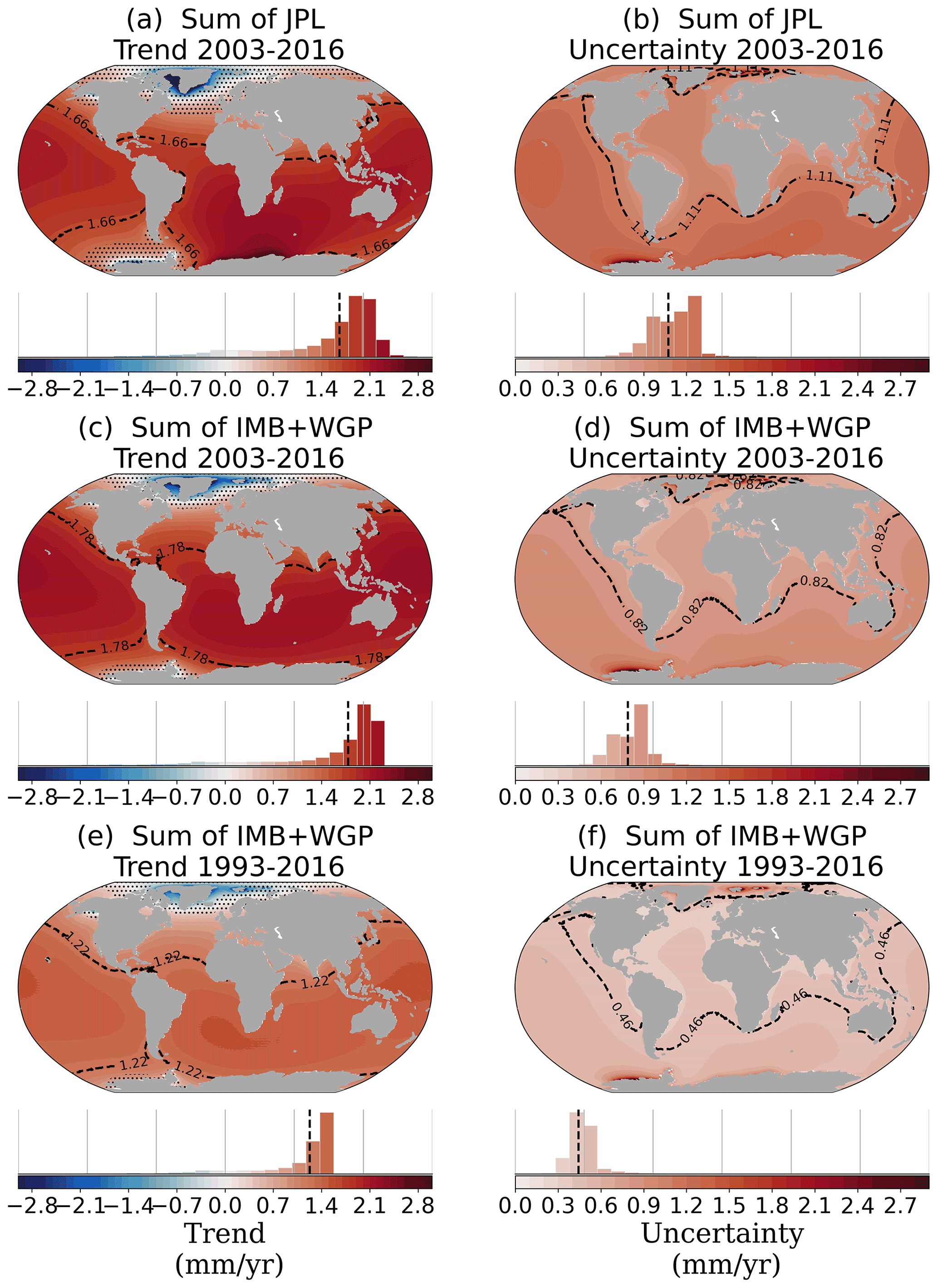
Figure 7Total GRD-induced SLC fields of the trend and uncertainty (mm yr−1) (AIS+GIS+LWS+Glaciers contributions; intrinsic + temporal + spatial uncertainties) for GRACE (a, b) and IMBIE+WaterGAP for 2003–2016 (c, d) and for 1993–2016 (e, f). Histograms underneath each map indicate the distribution of the regional values across the oceans, on which the 5th to 95th percentile range (90 % range) is based. Spatial average of the regional trend and uncertainty indicated by black dashed lines in the maps and bar charts. Regions with trends smaller than the 1-sigma uncertainty are indicated in the map with stipples.
3.6 Coastal examples
To further illustrate how the different contributions and uncertainties contribute to the total uncertainty budget, we selected 10 coastal cities around the world in which we break down the total uncertainty of GRD-induced SLC from 1993–2016 into the four contributions (Fig. 8a) and into the three types of uncertainties (Fig. 8b). We also show the different types of uncertainties for each of the contributions (Fig. 8c). As in Fig. 7, we show the IMB+WGP combination.
The large contribution of the LWS and temporal uncertainty to the uncertainty budget is highlighted in Fig. 8. Figure 8a shows that the LWS uncertainty plays an important role at all locations, being responsible for at least 50 % of the total uncertainty. While the temporal uncertainty is the main contribution of the LWS uncertainty (Fig. 8c), in some locations, such as Vancouver (Canada, location 1), Washington (US, location 3) and Tokyo (Japan, location 9), the spatial uncertainty is also important. Even without the contribution of LWS to the total uncertainty (Supplement Fig. B7b), the temporal uncertainty is still the main contributor. The intrinsic uncertainty (panel b) is fairly small in all locations, with an average contribution of 8 % for this dataset combination. However, for the JPL combination (Supplement Fig. B6), which has intrinsic uncertainty estimation for all contributions, the intrinsic uncertainty is responsible, on average, for 30 % of the total uncertainty, being more important than the spatial–structural one.
The second main contribution to the uncertainty budget comes from the AIS, except for Vancouver (Canada, location 1), for which the glaciers (GLA) contribute about 2 times more than AIS. The AIS uncertainty is mainly dominated by the intrinsic uncertainty, with the exception of Cape Town (South Africa, location 6), which is located within the large uncertainty contours of the spatial–structural uncertainty from AIS (see Fig. 5a). In general, the relative importance of GIS and GLA is fairly similar, with the exception of Vancouver (Canada, location 1) and Rotterdam (the Netherlands, location 5). In such locations, the GLA uncertainty is dominated by the spatial–structural contribution, while in all other locations the temporal uncertainty plays the most important role. On average, the GIS uncertainty is dominated by the intrinsic and temporal uncertainties rather than by spatial–structural uncertainty (panel c).
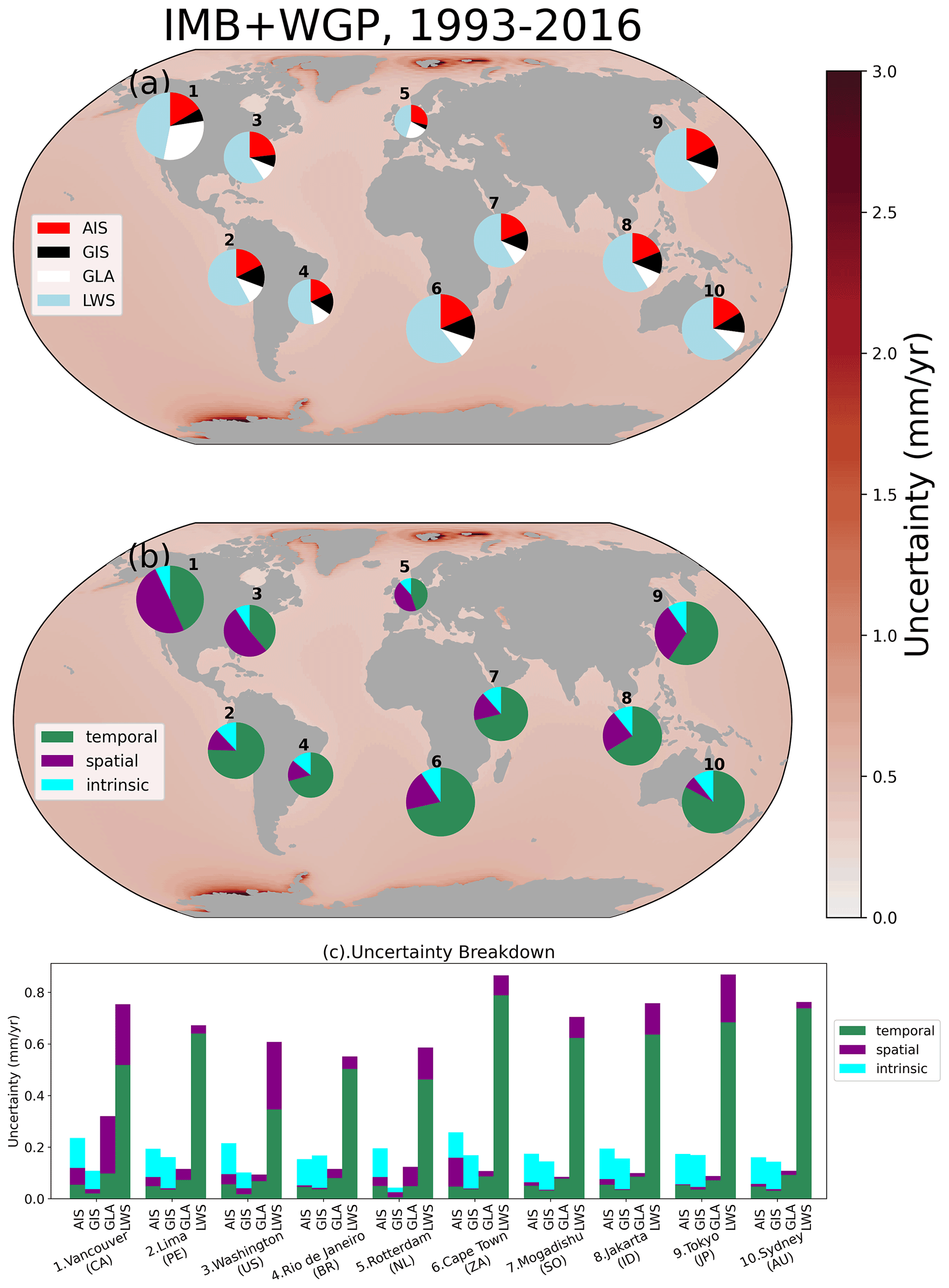
Figure 8Pie charts represent the total uncertainty separated by (a) contribution and (b) type of uncertainty, and the bars show the breakdown for each contribution (c). Background maps show the total GRD-induced uncertainty. The size of the pie charts is relative to the magnitude of the total uncertainty. Note that the uncertainties are combined in quadrature, so simply adding up the bars in panel (c) will not reflect the size of the pie charts in panels (a) and (b).
In this paper we investigated the regional GRD-induced SLC patterns associated with barystatic contribution to sea-level trends over 1993–2016 and 2003–2016, focusing on improving the understanding of the uncertainty budget. We showed how mass changes of glaciers, land water storage, and the Greenland and Antarctic ice sheets influence regional SLC by computing sea-level fingerprints. We considered three types of uncertainties in our budget: the determination of a linear trend (temporal), the spread around a central estimate as influenced by the distribution of mass change sources (spatial) and the uncertainty from the data/model itself (intrinsic).
The uncertainty budget is dominated by the temporal uncertainty, responsible on average for 65 % of the total uncertainty, while the spatial–structural and intrinsic uncertainties have smaller contributions of similar magnitude, responsible on average for 16 % and 18 % of the budget, respectively. The temporal uncertainties associated with the trend may represent real climatic signals and not only measurement errors. For example, the variability due to climatic oscillations, such as El Niño–Southern Oscillation (ENSO) and the Pacific Decadal Oscillation (PDO), may be reflected in the residuals of the time series, affecting the trend and its temporal uncertainties (Royston et al., 2018). As such climatic events influence not only mass change but also other drivers of sea-level change (e.g., thermal expansion) caution must be taken when using and comparing these uncertainties with those from other sea-level contributors. Despite the dataset-driven differences, for a given contribution all estimated trends agree within their respective 1-sigma uncertainties, for both regional and global mean values (Fig. 1, Supplement Table B1).
We find that the total GRD-induced sea-level trends range from −0.43 to 2.20 mm yr−1 for 2003–2016 and from −0.32 to 1.50 mm yr−1 for 1993–2016, depending on location, for the IMB+WGP combination, with spatial averages of 1.78 and 1.22 mm yr−1, respectively. The total uncertainty of the GRD-induced sea-level trend ranges from 0.63 to 0.98 mm yr−1 for 2003–2016 and from 0.38 to 0.60 mm yr−1 for 1993–2016 for the IMB+WGP combination, with spatial averages of 0.80 and 0.46 mm yr−1, respectively. While these uncertainty values may seem large compared to studies focusing on global changes alone (Horwath et al., 2021; Frederikse et al., 2020), other studies also found that regional uncertainties are higher than the previously published global mean rates (Prandi et al., 2021; Bos et al., 2014). For example, in a recent satellite altimetry sea-level change assessment, Prandi et al. (2021) found that the local sea-level trend uncertainty due to observational errors (i.e., intrinsic uncertainties) was about 2 times higher than the global mean sea-level trend uncertainty of Ablain et al. (2019). We note that the spatial average of the regional uncertainties (indicated by the black dashed line in the figures) is not equal to the uncertainty of the global mean barystatic SLC time series and trend. Consequently, the spatial averages will lead to larger values then the uncertainty of the global mean sea-level time series (see Fig. B5). Thus, one should not compare the value given here to characterize global mean sea-level changes with other studies focusing on the global mean (e.g. Horwath et al., 2021).
The GRD-induced sea-level trends clearly show the classical gravitational–rotational–deformational pattern, matching qualitatively with other fingerprints (e.g., Mitrovica et al., 2001; Riva et al., 2010; Hsu and Velicogna, 2017; Jeon et al., 2021). Our spatial–structural uncertainties highlight the effect of using a uniform mass change (i.e., only one value averaged over a region) compared to non-uniform local mass changes (Bamber and Riva, 2010; Mitrovica et al., 2011). For example, we show that different locations of mass changes can lead to deviations larger than 20 % for AIS (Fig. 5). As a consequence of the relatively low spatial resolution of the observations, the AIS is the second main contributor to the total GRD-induced uncertainty budget. We show that this effect is important not only for AIS but for all the GRD-induced SLC contributions.
The main source of uncertainty in the GRD-induced SLC is the temporal uncertainty from the land water storage (LWS) contribution, which is responsible for 35 %−60 % of the total uncertainty, depending on the region of interest. This is likely related to the (climate-driven) natural variability of LWS (Vishwakarma et al., 2021; Hamlington et al., 2017; Nerem et al., 2018), which is mainly driven by seasonal and interannual cycles (Cáceres et al., 2020). A method to deal with the natural variability of LWS would be to use different metrics than linear trends (Vishwakarma et al., 2021), such as time-varying trends based on a state space model (Frederikse et al., 2016; Vishwakarma et al., 2021). However, we choose to use linear trends in this study for the sake of accuracy, reproducibility and discussion. It has also been suggested that a more appropriate way of computing a meaningful linear trend from LWS is to incorporate this variability in the analysis (Vishwakarma et al., 2021), as we did by including the seasonal components in the functional model. Nonetheless, the LWS uncertainties related to the trend are still very high, suggesting that a period of 25 years (1993–2016) might still be too short to solve the low-frequency natural variability of LWS, particularly on (multi)-decadal timescales. Indeed, Humphrey et al. (2017) showed that removing the short-term climate-driven variability of the LWS signal yields a more robust long-term (>10 years) trend, with reduced uncertainties.
In this study we assessed the uncertainties related to the regional GRD-induced patterns associated with barystatic sea-level change, in particular their spatial distribution. The true uncertainty of ocean mass contribution to sea-level change is difficult to determine. Our approach of quantifying this uncertainty is to some extent conservative, as it results in larger uncertainties than in previous studies (e.g., Horwath et al., 2021). Nonetheless, we did assume independence of the different types of uncertainty and did not propagate GIA uncertainties into our fingerprints, which could lead to even larger uncertainties. Our results highlight that improving the spatial detail of land ice mass loss products, as well as determining more accurate land water storage trends, would lead to better SLC estimates. In addition, our findings can be used to inform projection frameworks. For example, we show that the distribution of ice in the Antarctic Ice Sheet has a significant impact on regional SLC, even in locations far from the ice sheets, such as the Netherlands. This means that, depending on the region of a collapse in the Antarctic Ice Sheet, the sea-level rise projections, which are often based on uniform ice sheet distributions and static fingerprints (e.g., Slangen et al., 2012; Jevrejeva et al., 2019), may have large regional deviations due to spatial differences in the mass source. Incorporating the insights of uncertainty assessments in sea-level frameworks (as in Larour et al., 2020) should eventually lead to better sea-level projections.
The datasets used in this paper are briefly described below. In-depth description of each dataset can be found in their respective references.
A1 GRACE mascon estimates
We use GRACE land mass concentration (mascons) solutions from two processing centers: RL06 v02 from CSR (Save et al., 2016; Save, 2020) and RL06 v02 from JPL (Watkins et al., 2015; Wiese et al., 2019). We chose to use the mascon solution instead of spherical harmonics to avoid the land–ocean leakage issue (Jeon et al., 2021; Chambers et al., 2007). The mascons include all mass changes in the Earth system, accounting for variations in land hydrology and in the cryosphere, as well as solid Earth motions (Adhikari et al., 2019). We do not, however, use the changes in the ocean, since we focus on land hydrology and cryosphere variations. CSR and JPL mascons are provided on 0.25 and 0.5 ∘ grids, respectively, even though the native resolution of the GRACE/GRACE-FO data is roughly 300 km (i.e., 3∘ equal-area mascons). The native resolution of CSR mascons are 1∘ equal-area grid and 3∘ for JPL mascons. Since the native resolution of GRACE observations about 300 km at the Equator (Tapley et al., 2004), the JPL mascons have independent solutions at each mascon center, with uncorrelated errors, while the CSR mascons are not fully independent and are expected to contain spatially correlated errors. Both mascons have been corrected for glacial isostatic adjustment (GIA) with the ICE6G-D model (Peltier et al., 2018) and for ocean and atmosphere dealiasing (AOD1B “GAD” fields). In addition, the JPL mascons use a Coastline Resolution Improvement (CRI) filter to separate land–ocean mass within the mascon (Wiese et al., 2016). Only the JPL mascons are provided with intrinsic uncertainty estimates (Wahr et al., 2006; Wiese et al., 2016). Both mascons are given with a monthly frequency, ranging from April 2002 to August 2020.
A2 IMBIE estimates
For both ice sheets we use the products of IMBIE (Shepherd et al., 2018, 2020), which combines several estimates (26 for GIS and 24 for AIS) of ice sheet mass balance derived from satellite altimetry, satellite gravimetry and the input–output method. The monthly datasets cover the period 1992–2017 and 1993–2018 for AIS and GIS, respectively. In addition to the total ice sheet mass balance, the GIS dataset also distinguishes between surface mass balance (GRE SMB) and dynamic ice discharge (GRE DYN). For the AIS, the data are subdivided in the main three drainage regions: West Antarctica, East Antarctica and the Antarctic Peninsula. The IMBIE estimates are provided with intrinsic uncertainty estimates, reflecting the combination of several different datasets.
A3 UCI AIS and GIS estimates
Using improved records of ice thickness, surface elevation, ice velocity and a surface mass balance model (RACMOv2.3), Mouginot et al. (2019) and Rignot et al. (2019) present yearly reconstructions of mass changes from the 1970s until 2017 and 2018 for the Greenland and Antarctic ice sheets, respectively. These GRACE-independent reconstructions agree, within uncertainties, with estimates from radar and laser altimetry and GRACE. The reconstructions are provided as the mean for each drainage basin, based on ice velocity data (18 basins for AIS, Rignot et al., 2011, and 6 for GIS, Mouginot and Rignot, 2019).
A4 WaterGAP hydrological model
We use the integrated version of the WaterGAP global hydrological model (Döll et al., 2003) v2.2d with a global glacier model (Marzeion et al., 2012), presented in Cáceres et al. (2020). The hydrological model uses a homogenized climate forcing from WFDEI (Weedon et al., 2014), with the precipitation correction of GPCC (Schneider et al., 2015). The model is provided on a 0.5∘ grid, covering all continental areas except for Antarctica. In order to consistently treat both ice sheets (GIS and AIS), we remove Greenland from the model. The WaterGAP model simulates human water use, daily water flows and water storage, taking into account dams and reservoirs based on the GRanD database (Lehner et al., 2011) and assuming that consumptive irrigation water use is 70 % of the optimal level in groundwater depletion areas. The glacier model computes mass changes for individual glaciers around the world (based on the Randolph Glacier Inventory; Pfeffer et al., 2014), including glacier surface mass balance, glacier geometry, air temperature and several others glacier-specific parameters and variables (Marzeion et al., 2012). The dataset is provided at a monthly frequency, from 1948–2016.
A5 PCR-GLOBWB hydrological model
The second global hydrological model included in our analysis is the PCRaster Global Water Balance 2 model (PCR- GLOBW, Sutanudjaja et al., 2018), which fully integrates different water uses, such as water demand, groundwater and surface water withdrawal, and water consumption, with the simulated hydrology. The model is forced with the W5E5 version 1 (Lange, 2019), covering the period 1979–2016. It provides monthly averages of total water storage thickness with a 5 arcmin resolution. Dams and reservoirs form the GRanD database (Lehner et al., 2011) are also included in the model. As this model does not explicitly resolve glaciers or include ice sheets, we mask out all the glaciated areas.
A6 Zemp 2019 glacier data
We use the yearly glacier mass loss estimates from Zemp et al. (2019) over the period 1961 to 2016. This dataset combines the temporal variability from the glaciological data, computed using a spatiotemporal variance decomposition, with the glacier-specific values of the geodetic observations. Both glaciological and geodetic observations come from the World Glacier Monitoring Service (WGMS, 2021). These combined data are then statistically extrapolated to the full glacier sample to assess regional mass changes, taking into account regional rates of area change. This dataset provides regional mass changes for the 19 regions of the Randolph Glacier Inventory (Consortium, 2017; Pfeffer et al., 2014). As the IMBIE estimates already account for peripheral glaciers to the ice sheets, we remove these from the Zemp dataset.
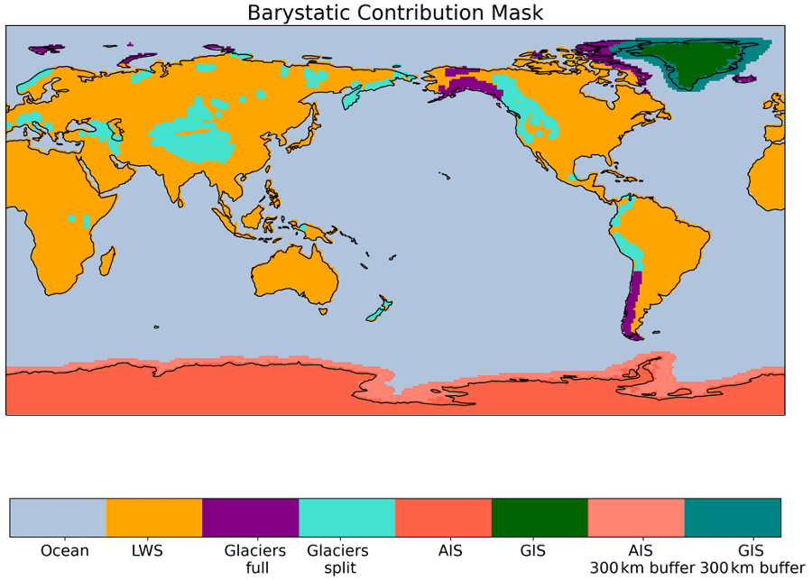
Figure B1Mask of the different contributions to barystatic sea-level change.
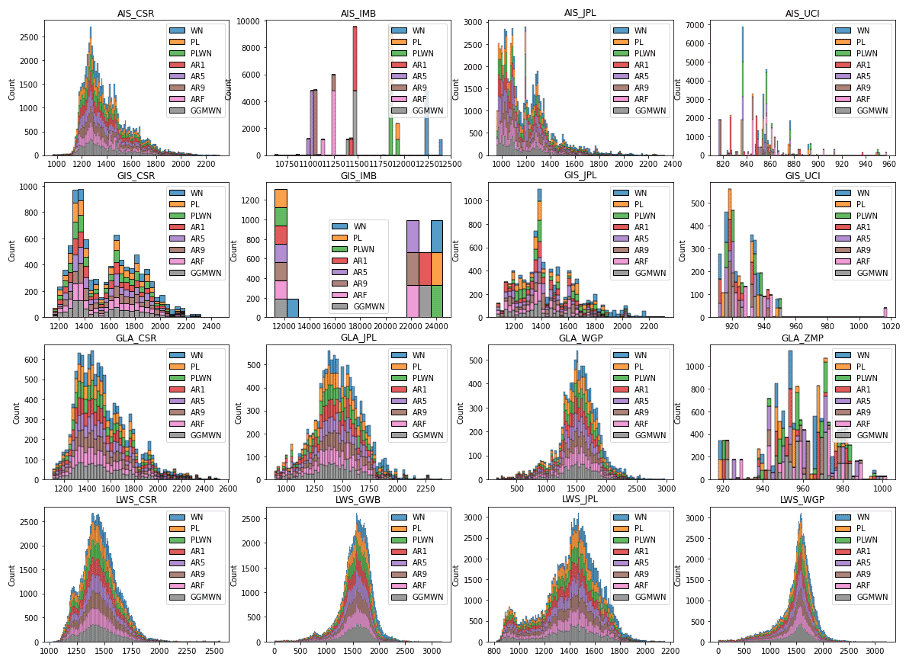
Figure B2Histogram of the modified Bayesian information criterion for each dataset, used to select the optimal noise models. The x axis shows the BIC score and the y axis the number of grid points (count). Note that all models have scores within the same range, showing that no model fails in capturing the signal of the observation.
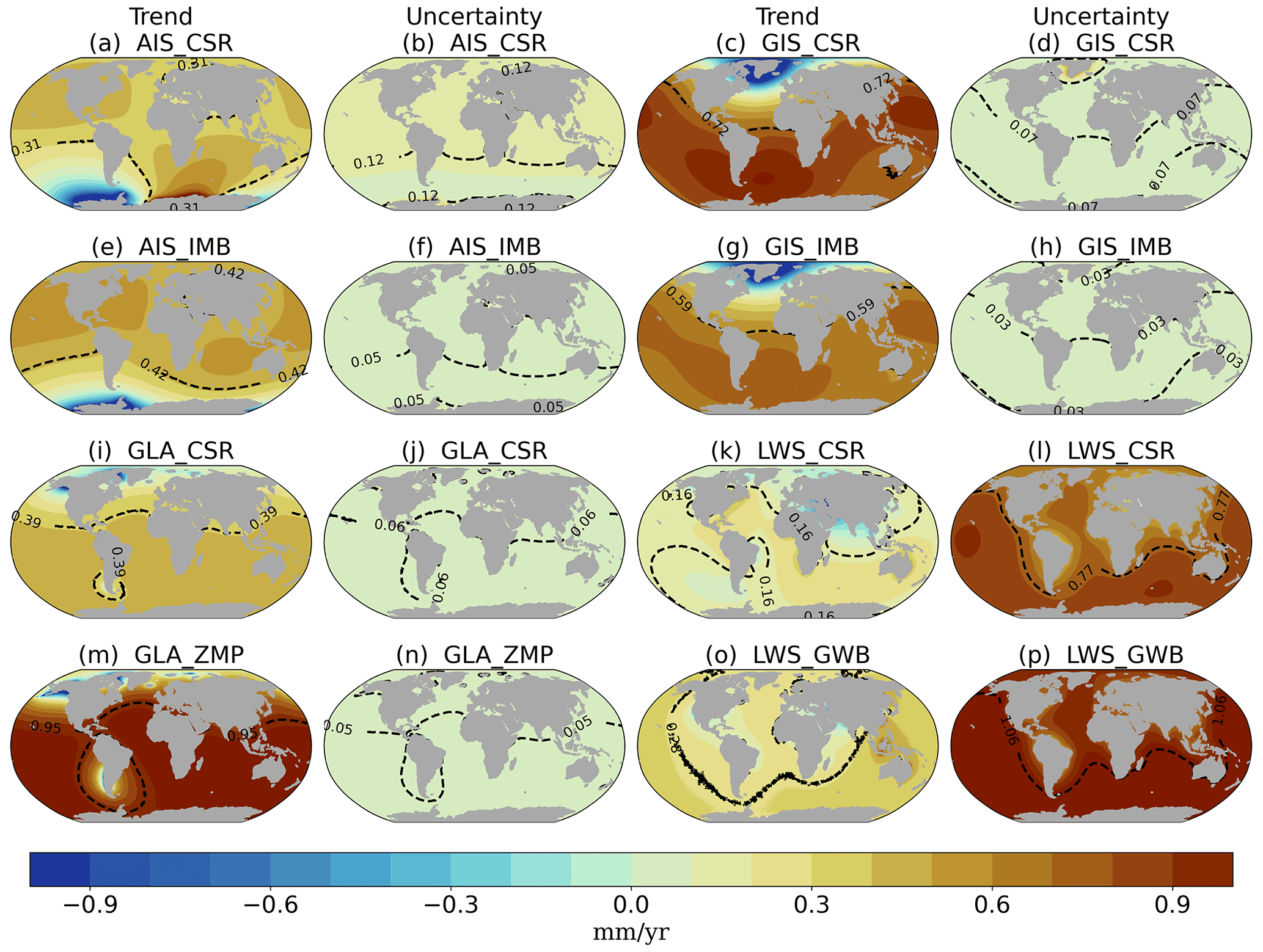
Figure B3GRD-induced sea-level trend and temporal uncertainty (mm yr−1) for GRACE (CSR) and independent combination (IMB + ZMP + GWB) for 2003–2016. The black dashed contour line and number indicate the spatial average of the regional trend and uncertainty. Complementary to trends and uncertainties of Fig. 4.
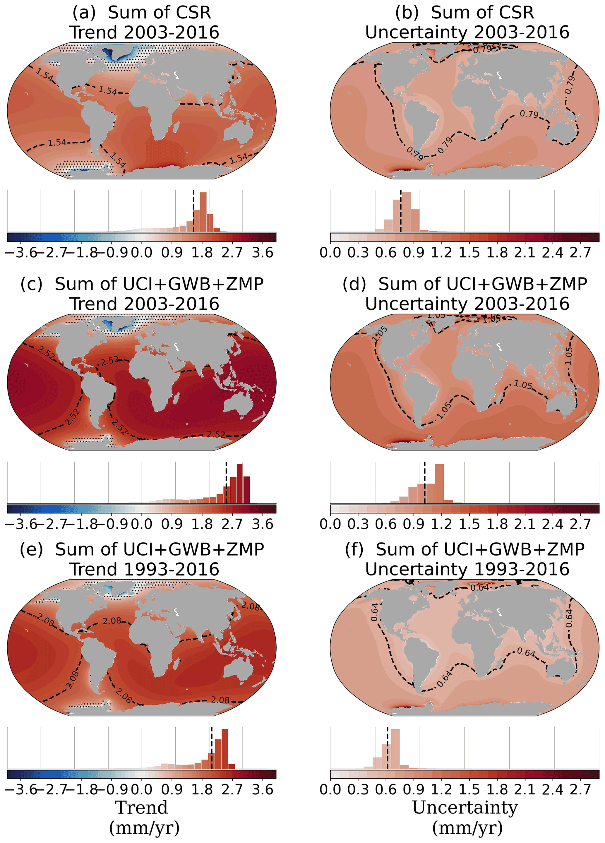
Figure B4Total GRD-induced SLC fields of the trend and uncertainty (mm yr−1) (AIS + GIS + LWS + glacier contributions; intrinsic + temporal + spatial uncertainties) for GRACE CRS (a, b) and UCI + GlobWEB + Zemp for 2005–2015 (c, d) and for 1993–2016 (e, f). Histograms underneath each map indicate the distribution of the regional values across the oceans. Spatial average of the regional trend and uncertainty indicated by black dashed lines in the maps and bar charts. Complementary to trends and uncertainties of Fig. 7.
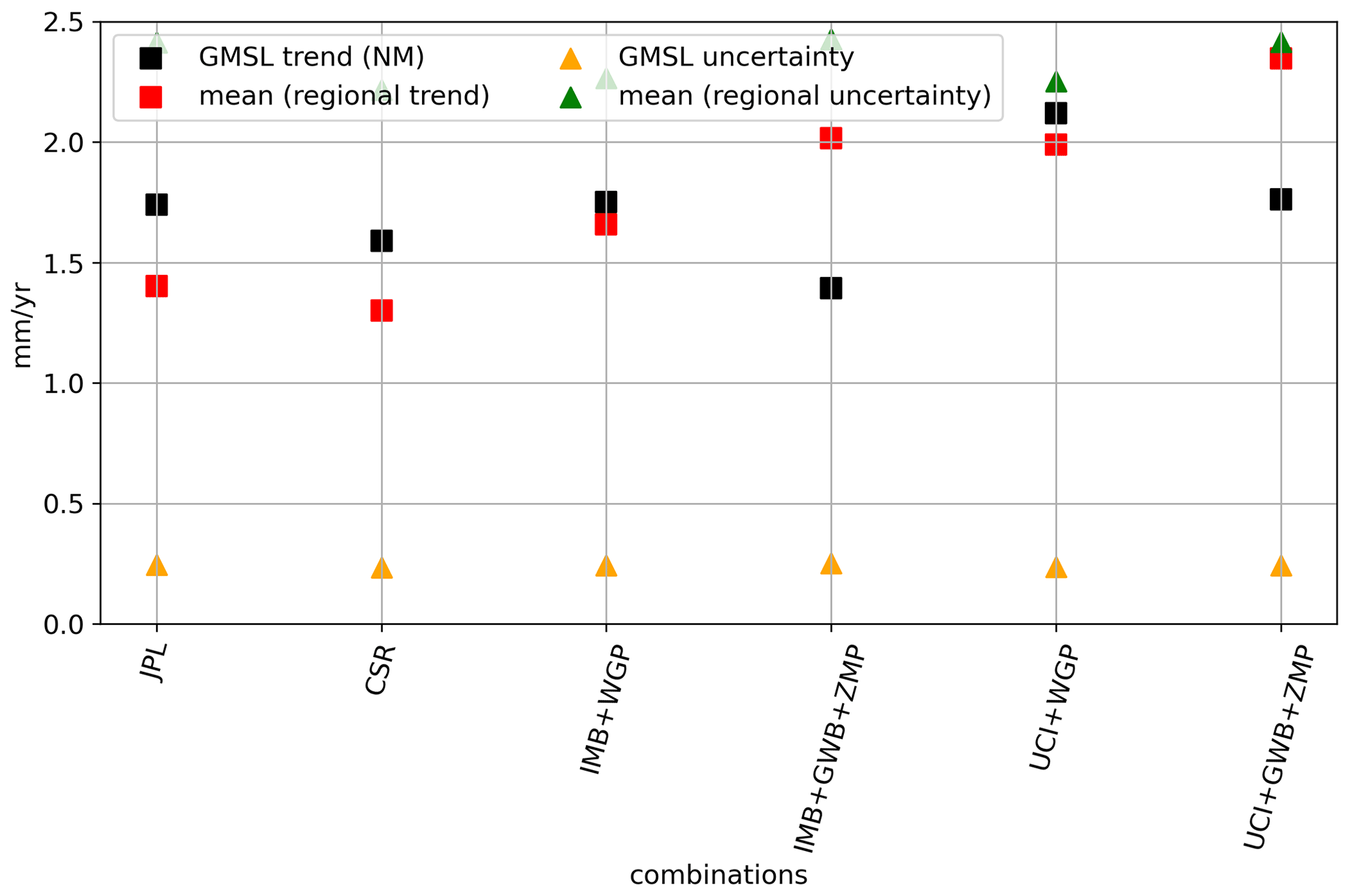
Figure B5Comparison of global mean sea-level trend (black squares) and uncertainty (yellow triangles) with the spatial average of the regional trend (red circles) and uncertainty (green upside down triangles) from 2003–2016. The difference between the GMSL trend and spatial average of the regional trend is due to the use of regionally different noise models (following selection of Fig. 3)

Figure B6Same as Fig. 8, for the JPL dataset, from 2003–2016.
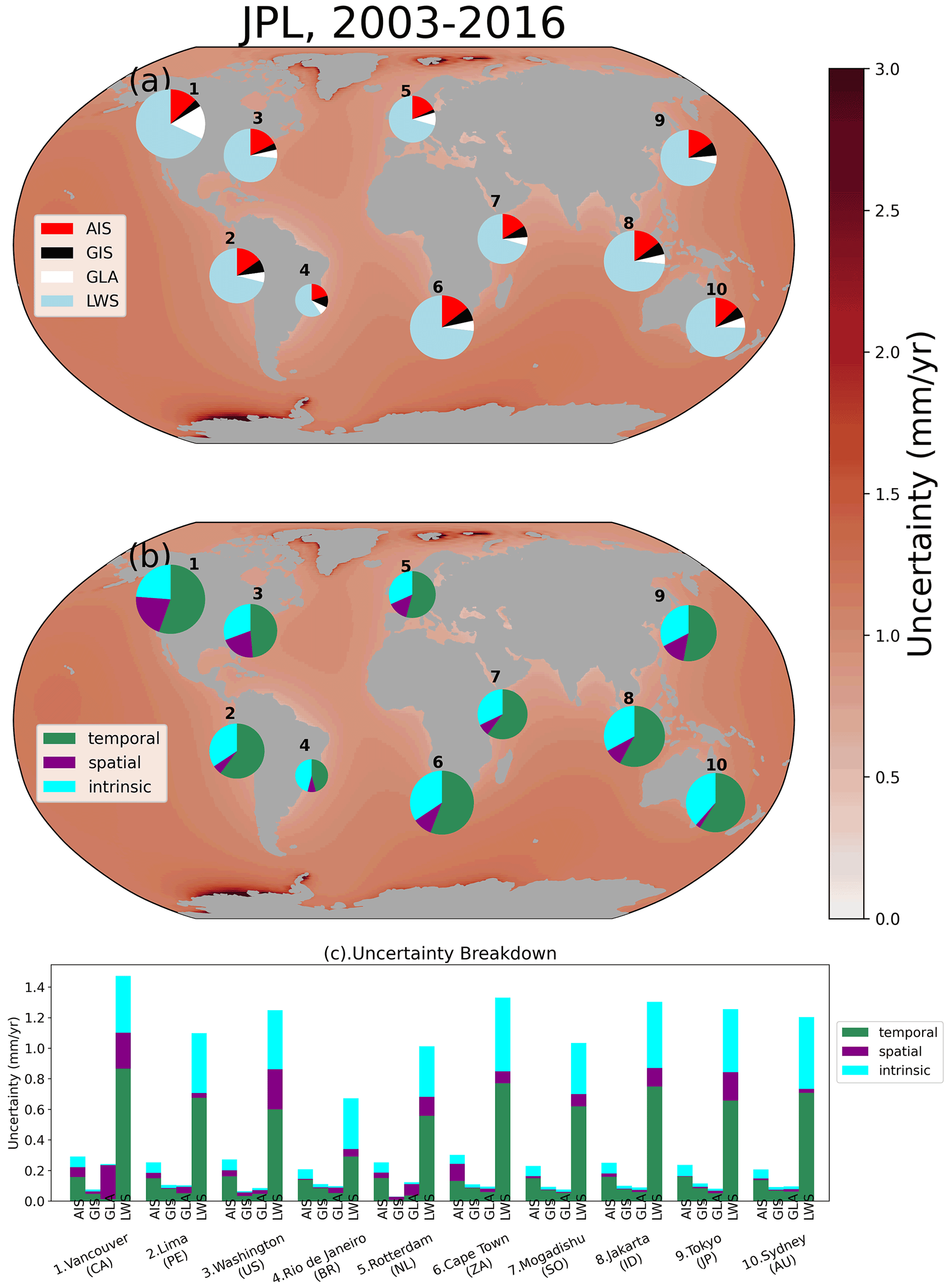
Figure B7Same as Fig. 8, but without the contribution of land water storage (LWS).
Table B1Global mean barystatic sea-level contributions and uncertainties. Note that these numbers may be different compared to the histograms of Fig. 7, which represent the spatial average of the regional trend and uncertainty. The difference between the trends is due to the use of noise models for the regional trend, against an ordinary least-squares fit for the global mean trend. Note that we remove the “spatial” part of the spatial–structural uncertainty of the regional assessment and define the structural uncertainty as the standard deviation of the trends for the same contribution.
The data used in this paper are available at the 4TU database (https://doi.org/10.4121/16778794; Camargo et al., 2021). The code for generating the figures is available at the GitHub repository https://github.com/carocamargo/barystaticSLC or https://doi.org/10.5281/zenodo.7093189 (carocamargo, 2022).
CMLC performed the research and drafted the article. CMLC, REMR and ABAS designed the study. All authors contributed to the interpretation of the results and the writing of the manuscript.
The contact author has declared that none of the authors has any competing interests.
Publisher’s note: Copernicus Publications remains neutral with regard to jurisdictional claims in published maps and institutional affiliations.
This research has been supported by the Netherlands Space Office (grant no. ALGWO.2017.002).
This paper was edited by Sagnik Dey and reviewed by Thomas Frederikse and one anonymous referee.
Ablain, M., Meyssignac, B., Zawadzki, L., Jugier, R., Ribes, A., Spada, G., Benveniste, J., Cazenave, A., and Picot, N.: Uncertainty in satellite estimates of global mean sea-level changes, trend and acceleration, Earth Syst. Sci. Data, 11, 1189–1202, https://doi.org/10.5194/essd-11-1189-2019, 2019. a, b, c
Abram, N., Gattuso, J.-P., Prakash, A., Cheng, L., Chidichimo, M., Crate, S., Enomoto, H., Garschagen, M., Gruber, N., Harper, S., Holland, E., Kudela, R., Rice, J., Steffen, K., and von Schuckmann, K.: Framing and Context of the Report, in: IPCC Special Report on the Ocean and Cryosphere in a Changing Climate, edited by: Pörtner, H.-O., Roberts, D. C., Masson-Delmotte, V., Zhai, P., Tignor, M., Poloczanska, E., Mintenbeck, K., Alegría, A., Nicolai, M., Okem, A., Petzold, J., Rama, B., and Weyer N. M., Cambridge University Press, Cambridge, UK and New York, NY, USA, pp. 73–129, https://doi.org/10.1017/9781009157964.003, 2019. a
Adhikari, S., Ivins, E. R., Frederikse, T., Landerer, F. W., and Caron, L.: Sea-level fingerprints emergent from GRACE mission data, Earth Syst. Sci. Data, 11, 629–646, https://doi.org/10.5194/essd-11-629-2019, 2019. a, b
Akaike, H.: A new look at the statistical model identification, IEEE Trans. Automat. Contr., 19, 716–723, https://doi.org/10.1109/TAC.1974.1100705, 1974. a
Amante, C. and Eakins, B. W.: ETOPO1 1 Arc‐Minute Global Relief Model: Procedures, Data Sources and Analysis, NOAA Technical Memorandum NESDIS NGDC‐24, National Geophysical Data Center, NOAA, [data set], https://doi.org/10.7289/V5C8276M, 2009. a
Bamber, J. and Riva, R.: The sea level fingerprint of recent ice mass fluxes, The Cryosphere, 4, 621–627, https://doi.org/10.5194/tc-4-621-2010, 2010. a, b, c
Blazquez, A., Meyssignac, B., Lemoine, J. M., Berthier, E., Ribes, A., and Cazenave, A.: Exploring the uncertainty in GRACE estimates of the mass redistributions at the Earth surface: Implications for the global water and sea level budgets, Geophys. J. Int., 215, 415–430, https://doi.org/10.1093/gji/ggy293, 2018. a
Bos, M. S., Fernandes, R. M., Williams, S. D., and Bastos, L.: Fast error analysis of continuous GNSS observations with missing data, J. Geodesy, 87, 351–360, https://doi.org/10.1007/s00190-012-0605-0, 2013. a, b, c, d, e, f, g
Bos, M. S., Williams, S. D., Araújo, I. B., and Bastos, L.: The effect of temporal correlated noise on the sea level rate and acceleration uncertainty, Geophys. J. Int., 196, 1423–1430, https://doi.org/10.1093/gji/ggt481, 2014. a, b
Burnham, K. P. and Anderson, D. R.: Model selection and multimodel inference a practical information-theoretic approach., vol. 2, Springer, New York, https://doi.org/10.1007/b97636, 2002. a
Cáceres, D., Marzeion, B., Malles, J. H., Gutknecht, B. D., Müller Schmied, H., and Döll, P.: Assessing global water mass transfers from continents to oceans over the period 1948–2016, Hydrol. Earth Syst. Sci., 24, 4831–4851, https://doi.org/10.5194/hess-24-4831-2020, 2020. a, b, c, d
Camargo, C. M. L., Riva, R. E. M., Hermans, T. H. J., and Slangen, A. B. A.: Exploring Sources of Uncertainty in Steric Sea‐Level Change Estimates, J. Geophys. Res.-Oceans, 125, 1–18, https://doi.org/10.1029/2020jc016551, 2020. a, b, c, d, e
Camargo, C. M. L., Hermans, T., Riva, R., and Slangen, A.: Data underlying the publication: Trends and Uncertainties of Mass-driven Sea-level Change in the Satellite Altimetry Era (1993–2016), 4TU.ResearchData [data set], https://doi.org/10.4121/16778794.v2, 2021. a
carocamargo: carocamargo/barystaticSLC: v1.0.0 – scripts for the published paper (v1.0.0), Zenodo [code], https://doi.org/10.5281/zenodo.7093189, 2022. a
Caron, L., Ivins, E. R., Larour, E., Adhikari, S., Nilsson, J., and Blewitt, G.: GIA Model Statistics for GRACE Hydrology, Cryosphere, and Ocean Science, Geophys. Res. Lett., 45, 2203–2212, https://doi.org/10.1002/2017GL076644, 2018. a
Chambers, D. P., Tamisiea, M. E., Nerem, R. S., and Ries, J. C.: Effects of ice melting on GRACE observations of ocean mass trends, Geophys. Res. Lett., 34, 1–5, https://doi.org/10.1029/2006GL029171, 2007. a, b
Church, J. A. and White, N. J.: A 20th century acceleration in global sea-level rise, Geophys. Res. Lett., 33, L01602, https://doi.org/10.1029/2005GL024826, 2006. a
Consortium: Randolph Glacier Inventory – A Dataset of Global Glacier Outlines: Version 6.0: Technical Report, Global Land Ice Measurements from Space, Colorado, USA, RGI [data set], https://doi.org/10.7265/N5-RGI-60, 2017. a, b
Crameri, F.: Scientific colour maps, Zenodo [data set], https://doi.org/10.5281/zenodo.1243862, 2018. a
Döll, P., Kaspar, F., and Lehner, B.: A global hydrological model for deriving water availability indicators: model tuning and validation, J. Hydrol., 260, 105–134, https://doi.org/10.1016/S0022-1694(02)00283-4, 2003. a
Dziewonski, A. and Anderson, D.: Preliminary reference Earth model, Phys. Earth Plan. Int., 25, 297–356, https://doi.org/10.17611/DP/9991844, 1981. a
Farrell, W. E. and Clark, J. A.: On Postglacial Sea Level, Geophys. J. Roy. Astronom. Soc., 46, 647–667, 1976. a, b
Fox-Kemper, B., Hewitt, H. T., Xiao, C., Aðalgeirsdóttir, G., Drijfhout, S. S., Edwards, T. L., N. R. Golledge, M. H., Kopp, R. E., Krinner, G., Mix, A., Notz, D., Nowicki, S., Nurhati, I. S., Ruiz, L., Sallée, J.-B., Slangen, A. B. A., and Yu, Y.: Ocean, Cryosphere and Sea Level Change, in: Climate Change 2021: The Physical Science Basis. Contribution of Working Group I to the Sixth Assessment Report of the Intergovernmental Panel on Climate Change, edited by: Masson-Delmotte, V., Zhai, P., Pirani, A., Connors, S. L., Péan, C., Berger, S., Caud, N., Chen, Y., Goldfarb, L., Gomis, M. I., Huang, M., Leitzell, K., Lonnoy, E., Matthews, J. B. R., Maycock, T. K., Waterfield, T., Yelekçi, O., Yu, R., and Zhou B., Cambridge University Press, Cambridge, United Kingdom and New York, NY, USA, 1211–1362 pp., https://doi.org/10.1017/9781009157896.011, 2021. a, b, c
Frederikse, T., Riva, R., Slobbe, C., Broerse, T., and Verlaan, M.: Estimating decadal variability in sea level from tide gauge records: An application to the North Sea, J. Geophys. Res.-Oceans, 121, 1529–1545, https://doi.org/10.1002/2015JC011174, 2016. a
Frederikse, T., Landerer, F. W., and Caron, L.: The imprints of contemporary mass redistribution on local sea level and vertical land motion observations, Solid Earth, 10, 1971–1987, https://doi.org/10.5194/se-10-1971-2019, 2019. a, b
Frederikse, T., Landerer, F., Caron, L., Adhikari, S., Parkes, D., Humphrey, V. W., Dangendorf, S., Hogarth, P., Zanna, L., Cheng, L., and Wu, Y. H.: The causes of sea-level rise since 1900, Nature, 584, 393–397, https://doi.org/10.1038/s41586-020-2591-3, 2020. a, b, c, d, e
Gomez, N., Mitrovica, J. X., Tamisiea, M. E., and Clark, P. U.: A new projection of sea level change in response to collapse of marine sectors of the Antarctic Ice Sheet, Geophys. J. Int., 180, 623–634, https://doi.org/10.1111/j.1365-246X.2009.04419.x, 2010. a
Gregory, J. M., Griffies, S. M., Hughes, C. W., Lowe, J. A., Church, J. A., Fukimori, I., Gomez, N., Kopp, R. E., Landerer, F., Cozannet, G. L., Ponte, R. M., Stammer, D., Tamisiea, M. E., and van de Wal, R. S.: Concepts and Terminology for Sea Level: Mean, Variability and Change, Both Local and Global, Surv. Geophys., 40, 1251–1289, https://doi.org/10.1007/s10712-019-09525-z, 2019. a, b
Hamlington, B. D., Reager, J. T., Lo, M. H., Karnauskas, K. B., and Leben, R. R.: Separating decadal global water cycle variability from sea level rise, Sci. Rep., 7, 995, https://doi.org/10.1038/s41598-017-00875-5, 2017. a
He, X., Bos, M. S., Montillet, J. P., and Fernandes, R. M. S.: Investigation of the noise properties at low frequencies in long GNSS time series, J. Geodesy, 93, 1271–1282, https://doi.org/10.1007/s00190-019-01244-y, 2019. a
Horwath, M., Gutknecht, B. D., Cazenave, A., Palanisamy, H. K., Marti, F., Marzeion, B., Paul, F., Le Bris, R., Hogg, A. E., Otosaka, I., Shepherd, A., Döll, P., Cáceres, D., Müller Schmied, H., Johannessen, J. A., Nilsen, J. E. Ø., Raj, R. P., Forsberg, R., Sandberg Sørensen, L., Barletta, V. R., Simonsen, S. B., Knudsen, P., Andersen, O. B., Ranndal, H., Rose, S. K., Merchant, C. J., Macintosh, C. R., von Schuckmann, K., Novotny, K., Groh, A., Restano, M., and Benveniste, J.: Global sea-level budget and ocean-mass budget, with a focus on advanced data products and uncertainty characterisation, Earth Syst. Sci. Data, 14, 411–447, https://doi.org/10.5194/essd-14-411-2022, 2022. a, b, c, d, e
Hsu, C. W. and Velicogna, I.: Detection of sea level fingerprints derived from GRACE gravity data, Geophys. Res. Lett., 44, 8953–8961, https://doi.org/10.1002/2017GL074070, 2017. a, b
Hughes, C. W. and Williams, S. D.: The color of sea level: Importance of spatial variations in spectral shape for assessing the significance of trends, J. Geophys. Res.-Oceans, 115, C10048, https://doi.org/10.1029/2010JC006102, 2010. a, b, c
Hugonnet, R., McNabb, R., Berthier, E., Menounos, B., Nuth, C., Girod, L., Farinotti, D., Huss, M., Dussaillant, I., Brun, F., and Kääb, A.: Accelerated global glacier mass loss in the early twenty-first century, Nature, 592, 726–731, https://doi.org/10.1038/s41586-021-03436-z, 2021. a, b
Humphrey, V. and Gudmundsson, L.: GRACE-REC: a reconstruction of climate-driven water storage changes over the last century, Earth Syst. Sci. Data, 11, 1153–1170, https://doi.org/10.5194/essd-11-1153-2019, 2019. a
Humphrey, V., Gudmundsson, L., and Seneviratne, S. I.: A global reconstruction of climate-driven subdecadal water storage variability, Geophys. Res. Lett., 44, 2300–2309, https://doi.org/10.1002/2017GL072564, 2017. a
Jeon, T., Seo, K. W., Kim, B. H., Kim, J. S., Chen, J., and Wilson, C. R.: Sea level fingerprints and regional sea level change, Earth Planet. Sci. Lett., 567, 116985, https://doi.org/10.1016/j.epsl.2021.116985, 2021. a, b
Jevrejeva, S., Frederikse, T., Kopp, R. E., Le Cozannet, G., Jackson, L. P., and van de Wal, R. S. W.: Probabilistic Sea Level Projections at the Coast by 2100, Surv. Geophys., 40, 1673–1696, 2019. a
Landerer, F. W., Flechtner, F. M., Save, H., Webb, F. H., Bandikova, T., Bertiger, W. I., Bettadpur, S. V., Byun, S. H., Dahle, C., Dobslaw, H., Fahnestock, E., Harvey, N., Kang, Z., Kruizinga, G. L., Loomis, B. D., McCullough, C., Murböck, M., Nagel, P., Paik, M., Pie, N., Poole, S., Strekalov, D., Tamisiea, M. E., Wang, F., Watkins, M. M., Wen, H. Y., Wiese, D. N., and Yuan, D. N.: Extending the Global Mass Change Data Record: GRACE Follow-On Instrument and Science Data Performance, Geophys. Res. Lett., 47, 1–10, https://doi.org/10.1029/2020GL088306, 2020. a
Lange, S.: WFDE5 over land merged with ERA5 over the ocean (W5E5), V. 1.0, GFZ Data Services [data set], https://doi.org/10.5880/pik.2019.023, 2019. a
Larour, E., Ivins, E. R., and Adhikari, S.: Should coastal planners have concern over where land ice is melting?, Sci. Adv., 3, 1–9, https://doi.org/10.1126/sciadv.1700537, 2017. a
Larour, E., Caron, L., Morlighem, M., Adhikari, S., Frederikse, T., Schlegel, N.-J., Ivins, E., Hamlington, B., Kopp, R., and Nowicki, S.: ISSM-SLPS: geodetically compliant Sea-Level Projection System for the Ice-sheet and Sea-level System Model v4.17, Geosci. Model Dev., 13, 4925–4941, https://doi.org/10.5194/gmd-13-4925-2020, 2020. a
Lehner, B., Liermann, C. R., Revenga, C., Vörösmarty, C., Fekete, B., Crouzet, P., Döll, P., Endejan, M., Frenken, K., Magome, J., Nilsson, C., Robertson, J. C., Rödel, R., Sindorf, N., and Wisser, D.: High-resolution mapping of the world's reservoirs and dams for sustainable river-flow management, Front. Ecol. Environ., 9, 494–502, https://doi.org/10.1890/100125, 2011. a
Lin, Y., Hibbert, F. D., Whitehouse, P. L., Woodroffe, S. A., Purcell, A., Shennan, I., and Bradley, S. L.: A reconciled solution of Meltwater Pulse 1A sources using sea-level fingerprinting, Nat. Commun., 12, 2015, https://doi.org/10.1038/s41467-021-21990-y, 2021. a
MacIntosh, C. R., Merchant, C. J., and von Schuckmann, K.: Uncertainties in Steric Sea Level Change Estimation During the Satellite Altimeter Era: Concepts and Practices, Surv. Geophys., 38, 59–87, 2017. a
Marzeion, B., Jarosch, A. H., and Hofer, M.: Past and future sea-level change from the surface mass balance of glaciers, The Cryosphere, 6, 1295–1322, https://doi.org/10.5194/tc-6-1295-2012, 2012. a, b, c
Milne, G. A. and Mitrovica, J. X.: Postglacial sea-level change on a rotating Earth, Geophys. J. Int., 133, 1–19, https://doi.org/10.1046/j.1365-246X.1998.1331455.x, 1998. a
Mitrovica, J., Tamisiea, M., Davis, J., and Milne, G.: Recent mass balance of polar ice sheets inferred from patterns of global sea-level change, Nature, 409, 1026–1029, https://doi.org/10.1038/35059054, 2001. a, b, c, d, e
Mitrovica, J., Gomez, N., Morrow, E., Hay, C., Latychev, K., and Tamisiea, M.: On the robustness of predictions of sea level fingerprints, Geophys. J. Int., 187, 729–742, https://doi.org/10.1111/j.1365-246X.2011.05090.x, 2011. a, b, c
Mitrovica, J. X. and Peltier, W. R.: On Postglacial Geoid Subsidence Over the Equatorial Oceans, J. Geophys. Res., 96, 20053–20071, https://doi.org/10.1029/91JB01284, 1991. a
Mouginot, J. and Rignot, E.: Glacier Catchments/Basins for the Greenland Ice Sheet, Dryad [data set], https://doi.org/10.7280/D1WT11, 2019. a, b
Mouginot, J., Rignot, E., Bjørk, A. A., van den Broeke, M., Millan, R., Morlighem, M., Noël, B., Scheuchl, B., and Wood, M.: Supplement of Forty-six years of Greenland Ice Sheet mass balance from 1972 to 2018, Proc. Natl. Acad. Sci. USA, 116, 9239–9244, https://doi.org/10.1073/pnas.1904242116, 2019. a, b
Nerem, R. S., Beckley, B. D., Fasullo, J. T., Hamlington, B. D., Masters, D., and Mitchum, G. T.: Climate-change-driven accelerated sea-level rise detected in the altimeter era, Proc. Natl. Acad. Sci., 115, 2022–2025, https://doi.org/10.1073/pnas.1717312115, 2018. a
Nicholls, R., Wong, P., Burkett, V., Codignotto, J., Hay, J., McLean, R., Ragoonaden, S., and Woodroffe, C.: Coastal systems and low-lying areas, in: Climate Change 2007: Impacts, Adaptation and Vulnerability. Contribution of Working Group II to the Fourth Assessment Report of the Intergovernmental Panel on Climate Change, Cambridge University Press, 164, 22225, https://ro.uow.edu.au/scipapers/164, 2007. a
Oppenheimer, M., Abdelgawad, A., Hay, J., Glavovic, B., Cai, R., Marzeion, B., Hinkel, J., Cifuentes-Jara, M., Meyssignac, B., Van De Wal, R., DeConto, R., Sebesvari, Z., Magnan, A., and Ghosh, Hay, T. J., Isla, F., Marzeion, B., Meyssignac, B., and Sebesvari, Z.: Sea Level Rise and Implications for Low-Lying Islands, Coasts and Communities, in: IPCC Special Report on the Ocean and Cryosphere in a Changing Climate, edited by: Pörtner, H.-O., Roberts, D. C., Masson-Delmotte, V., Zhai, P., Tignor, M., Poloczanska, E., Mintenbeck, K., Alegría, A., Nicolai, M., Okem, A., Petzold, J., Rama, B., Weyer, N. M., Cambridge University Press, Cambridge, UK and New York, NY, USA, 321–445, https://doi.org/10.1017/9781009157964.006, 2019. a
Palmer, M. D., Domingues, C. M., Slangen, A. B. A., and Boeira Dias, F.: An ensemble approach to quantify global mean sea-level rise over the 20th century from tide gauge reconstructions, Environ. Res. Lett., 16, 044043, https://doi.org/10.1088/1748-9326/abdaec, 2021. a, b, c, d, e
Peltier, W. R., Argus, D. F., and Drummond, R.: Comment on “An Assessment of the ICE-6G_C (VM5a) Glacial Isostatic Adjustment Model” by Purcell et al., J. Geophys. Res.-Solid Earth, 123, 2019–2028, https://doi.org/10.1002/2016JB013844, 2018. a, b
Pfeffer, W. T., Arendt, A. A., Bliss, A., Bolch, T., Cogley, J. G., Gardner, A. S., Hagen, J.-O., Hock, R., Kaser, G., Kienholz, C., and et al.: The Randolph Glacier Inventory: a globally complete inventory of glaciers, J. Glaciol., 60, 537–552, https://doi.org/10.3189/2014JoG13J176, 2014. a, b
Prandi, P., Meyssignac, B., Ablain, M., Spada, G., Ribes, A., and Benveniste, J.: Local sea level trends, accelerations and uncertainties over 1993–2019, Sci. Data, 8, 1–12, https://doi.org/10.1038/s41597-020-00786-7, 2021. a, b, c, d
Reager, J. T., Gardner, A. S., Famiglietti, J. S., Wiese, D. N., Eicker, A., and Lo, M. H.: A decade of sea level rise slowed by climate-driven hydrology, Science, 351, 699–703, https://doi.org/10.1126/science.aad8386, 2016. a, b
Rignot, E., Mouginot, J., and Scheuchl, B.: Antarctic grounding line mapping from differential satellite radar interferometry, Geophys. Res. Lett., 38, L10504, https://doi.org/10.1029/2011GL047109, 2011. a, b
Rignot, E., Mouginot, J., Scheuchl, B., Van Den Broeke, M., Van Wessem, M. J., and Morlighem, M.: Four decades of Antarctic ice sheet mass balance from 1979–2017, Proc. Natl. Acad. Sci. USA, 116, 1095–1103, https://doi.org/10.1073/pnas.1812883116, 2019. a, b
Riva, R., Bamber, J., Lavallee, D., and Wouters, B.: Sea-level fingerprint of continental water and ice mass change from GRACE, Geophys. Res. Lett., 37, 1–6, https://doi.org/10.1029/2010GL044770, 2010. a, b
Royston, S., Watson, C. S., Legrésy, B., King, M. A., Church, J. A., and Bos, M. S.: Sea-Level Trend Uncertainty With Pacific Climatic Variability and Temporally-Correlated Noise, J. Geophys. Res.-Oceans, 123, 1978–1993, https://doi.org/10.1002/2017JC013655, 2018. a, b, c
Save, H.: CSR GRACE and GRACE-FO RL06 Mascon Solutions v02, CSR [data set], https://doi.org/10.15781/cgq9-nh24, 2020. a, b
Save, H., Bettadpur, S., and Tapley, B. D.: High-resolution CSR GRACE RL05 mascons, J. Geophys. Res.-Solid Earth, 121, 7547–7569, https://doi.org/10.1002/2017JB015312, 2016. a, b, c, d
Schneider, U., Becker, A., Finger, P., Meyer-Christoffer, A., Rudolf, B., and Ziese, M.: GPCC full data reanalysis version 7.0 at 0.5∘: monthly land-surface precipitation from rain-gauges built on GTS-based and historic data, Global Precipitation Climatology Centre (GPCC), https://doi.org/10.5676/dwd_gpcc/fd_m_v7_050, http://gpcc.dwd.de/ (last access: 19 September 2022), 2015. a
Schwarz, G.: Estimating the Dimension of a Model, The Annals of Statistics, 6, 461–464, 1978. a
Shepherd, A., Ivins, E., Rignot, E., Smith, B., Van Den Broeke, M., Velicogna, I., Whitehouse, P., Briggs, K., Joughin, I., Krinner, G., Nowicki, S., Payne, T., Scambos, T., Schlegel, N., Geruo, A., Agosta, C., Ahlstrøm, A., Babonis, G., Barletta, V., Blazquez, A., Bonin, J., Csatho, B., Cullather, R., Felikson, D., Fettweis, X., Forsberg, R., Gallee, H., Gardner, A., Gilbert, L., Groh, A., Gunter, B., Hanna, E., Harig, C., Helm, V., Horvath, A., Horwath, M., Khan, S., Kjeldsen, K. K., Konrad, H., Langen, P., Lecavalier, B., Loomis, B., Luthcke, S., McMillan, M., Melini, D., Mernild, S., Mohajerani, Y., Moore, P., Mouginot, J., Moyano, G., Muir, A., Nagler, T., Nield, G., Nilsson, J., Noel, B., Otosaka, I., Pattle, M. E., Peltier, W. R., Pie, N., Rietbroek, R., Rott, H., Sandberg-Sørensen, L., Sasgen, I., Save, H., Scheuchl, B., Schrama, E., Schröder, L., Seo, K. W., Simonsen, S., Slater, T., Spada, G., Sutterley, T., Talpe, M., Tarasov, L., Van De Berg, W. J., Van Der Wal, W., Van Wessem, M., Vishwakarma, B. D., Wiese, D., and Wouters, B.: Mass balance of the Antarctic Ice Sheet from 1992 to 2017, Nature, 558, 219–222, https://doi.org/10.1038/s41586-018-0179-y, 2018. a, b, c
Shepherd, A., Ivins, E., Rignot, E., Smith, B., van den Broeke, M., Velicogna, I., Whitehouse, P., Briggs, K., Joughin, I., Krinner, G., Nowicki, S., Payne, T., Scambos, T., Schlegel, N., A, G., Agosta, C., Ahlstrøm, A., Babonis, G., Barletta, V. R., Bjørk, A. A., Blazquez, A., Bonin, J., Colgan, W., Csatho, B., Cullather, R., Engdahl, M. E., Felikson, D., Fettweis, X., Forsberg, R., Hogg, A. E., Gallee, H., Gardner, A., Gilbert, L., Gourmelen, N., Groh, A., Gunter, B., Hanna, E., Harig, C., Helm, V., Horvath, A., Horwath, M., Khan, S., Kjeldsen, K. K., Konrad, H., Langen, P. L., Lecavalier, B., Loomis, B., Luthcke, S., McMillan, M., Melini, D., Mernild, S., Mohajerani, Y., Moore, P., Mottram, R., Mouginot, J., Moyano, G., Muir, A., Nagler, T., Nield, G., Nilsson, J., Noël, B., Otosaka, I., Pattle, M. E., Peltier, W. R., Pie, N., Rietbroek, R., Rott, H., Sandberg Sørensen, L., Sasgen, I., Save, H., Scheuchl, B., Schrama, E., Schröder, L., Seo, K. W., Simonsen, S. B., Slater, T., Spada, G., Sutterley, T., Talpe, M., Tarasov, L., van de Berg, W. J., van der Wal, W., van Wessem, M., Vishwakarma, B. D., Wiese, D., Wilton, D., Wagner, T., Wouters, B., and Wuite, J.: Mass balance of the Greenland Ice Sheet from 1992 to 2018, Nature, 579, 233–239, https://doi.org/10.1038/s41586-019-1855-2, 2020. a, b, c
Simon, K. M. and Riva, R. E.: Uncertainty Estimation in Regional Models of Long-Term GIA Uplift and Sea Level Change: An Overview, J. Geophys. Res.-Solid Earth, 125, e2019JB018983, https://doi.org/10.1029/2019JB018983, 2020. a
Slangen, A. B. A., Katsman, C. A., van de Wal, R. S. W., Vermeersen, L. L. A., and Riva, R. E. M.: Towards regional projections of twenty-first century sea-level change based on IPCC SRES scenarios, Clim. Dynam., 38, 1191–1209, 2012. a, b
Slangen, A. B. A., van de Wal, R. S. W., Wada, Y., and Vermeersen, L. L. A.: Comparing tide gauge observations to regional patterns of sea-level change (1961–2003), Earth Syst. Dynam., 5, 243–255, https://doi.org/10.5194/esd-5-243-2014, 2014. a, b
Sutanudjaja, E. H., van Beek, R., Wanders, N., Wada, Y., Bosmans, J. H. C., Drost, N., van der Ent, R. J., de Graaf, I. E. M., Hoch, J. M., de Jong, K., Karssenberg, D., López López, P., Peßenteiner, S., Schmitz, O., Straatsma, M. W., Vannametee, E., Wisser, D., and Bierkens, M. F. P.: PCR-GLOBWB 2: a 5 arcmin global hydrological and water resources model, Geosci. Model Dev., 11, 2429–2453, https://doi.org/10.5194/gmd-11-2429-2018, 2018. a, b
Tamisiea, M. E. and Mitrovica, J. X.: The Moving boundaries of Sea Level Change, Oceanography, 24, 24–39, https://doi.org/10.5670/oceanog.2011.25, 2011. a, b
Tapley, B. D., Bettadpur, S., Watkins, M., and Reigber, C.: The gravity recovery and climate experiment: Mission overview and early results, Geophys. Res. Lett., 31, L09607, https://doi.org/10.1029/2004GL019920, 2004. a, b, c, d
Taylor, J. R.: An introduction to error analysis : the study of uncertainties in physical measurements, University Science Books, Sausalito, California, ISBN 0935702423, 1997. a
Thorne, P.: Global surface temperatures, in: Climate Change, Observed Impacts on Planet Earth, 2021, 95–109, https://doi.org/10.1016/b978-0-12-821575-3.00005-0, 2021. a, b
Thorne, P., Parkes, D., Christy, J., and Mears, C.: Lessons from Upper-Air Temperature Records, Am. Meteorol. Soc., 86, 1437–1442, https://doi.org/10.1175/BAMS-86-10-1437, 2005. a
Thyng, K. M., Greene, C. A., Hetland, R. D., Zimmerle, H. M., and DiMarco, S. F.: True colors of oceanography, Oceanography, 3, 9–13, https://doi.org/10.5670/oceanog.2016.66, 2016. a
Vishwakarma, B. D., Bates, P., Sneeuw, N., Westaway, R. M., and Bamber, J. L.: Re-assessing global water storage trends from GRACE time series, Environ. Res. Lett., 16, 034005, https://doi.org/10.1088/1748-9326/abd4a9, 2021. a, b, c, d
Wahr, J., Swenson, S., and Velicogna, I.: Accuracy of GRACE mass estimates, Geophys. Res. Lett., 33, L06401, https://doi.org/10.1029/2005GL025305, 2006. a, b, c, d, e
Watkins, M. M., Wiese, D. N., Yuan, D.-N., Boening, C., and Landerer, F. W.: Improved methods for observing Earth's time variable mass distribution with GRACE using spherical cap mascons, J. Geosci. Res.-Solid Earth, 120, 1648–2671, https://doi.org/10.1002/2014JB011547, 2015. a, b, c, d
WCRP Global Sea Level Budget Group: Global sea-level budget 1993–present, Earth Syst. Sci. Data, 10, 1551–1590, https://doi.org/10.5194/essd-10-1551-2018, 2018. a, b
Weedon, G. P., Balsamo, G., Bellouin, N., Gomes, S., Best, M. J., and Viterbo, P.: The WFDEI meteorological forcing data set: WATCH Forcing Data methodology applied to ERA-Interim reanalysis data, Water Resour. Res., 50, 7505–7514, https://doi.org/10.1002/2014WR015638, 2014. a
WGMS: Fluctuations of Glaciers Database, World Glacier Monitoring Service, Zurich, Switzerland, https://doi.org/10.5904/wgms-fog-2021-05, 2021. a
Wiese, D. N., Landerer, F. W., and Watkins, M. M.: Quantifying and reducing leakage errors in the JPL RL05M GRACE mascon solution, Water Resour. Res., 52, 7490–7502 , https://doi.org/10.1002/2016WR019344, 2016. a, b, c
Wiese, D. N., Yuan, D.-N., Boening, C., Landerer, F. W., and Watkins, M. M.: JPL GRACE Mascon Ocean, Ice, and Hydrology Equivalent Water Height RL06 CRI Filtered Version 2 PO.DAAC, CA, USA, JPL [data set], https://doi.org/10.5067/TEMSC-3JC62, 2019. a, b
Wigley, T. M. L.: The Climate Change Commitment, Science, 307, 1766–1769, https://doi.org/10.1126/science.1103934, 2005. a
Wouters, B., Gardner, A. S., and Moholdt, G.: Global Glacier Mass Loss During the GRACE Satellite Mission (2002–2016), Front. Earth Sci., 7, 1–11, https://doi.org/10.3389/feart.2019.00096, 2019. a
Zemp, M., Huss, M., Thibert, E., Eckert, N., McNabb, R., Huber, J., Barandun, M., Machguth, H., Nussbaumer, S. U., Gärtner-Roer, I., Thomson, L., Paul, F., Maussion, F., Kutuzov, S., and Cogley, J. G.: Global glacier mass changes and their contributions to sea-level rise from 1961 to 2016, Nature, 568, 382–386, https://doi.org/10.1038/s41586-019-1071-0, 2019. a, b