the Creative Commons Attribution 4.0 License.
the Creative Commons Attribution 4.0 License.
 | 18 Jan 2021
Stratospheric ozone and quasi-biennial oscillation (QBO) interaction with the tropical troposphere on intraseasonal and interannual timescales: a normal-mode perspective
Breno Raphaldini
André S. W. Teruya
Pedro Leite da Silva Dias
Lucas Massaroppe
Daniel Yasumasa Takahashi
The Madden–Julian oscillation (MJO) is the main controller of the weather in the tropics on intraseasonal timescales, and recent research provides evidence that the quasi-biennial oscillation (QBO) influences the MJO interannual variability. However, the physical mechanisms behind this interaction are not completely understood. Recent studies on the normal-mode structure of the MJO indicate the contribution of global-scale Kelvin and Rossby waves. In this study we test whether these MJO-related normal modes are affected by the QBO and stratospheric ozone. The partial directed coherence method was used and enabled us to probe the direction and frequency of the interactions. It was found that equatorial stratospheric ozone and stratospheric zonal winds are connected with the MJO at periods of 1–2 months and 1.5–2.5 years. We explore the role of normal-mode interactions behind the stratosphere–troposphere coupling by performing a linear regression between the MJO–QBO indices and the amplitudes of the normal modes of the atmosphere obtained by projections on a normal-mode basis using ERA-Interim reanalysis data. The MJO is dominated by symmetric Rossby modes but is also influenced by Kelvin and asymmetric Rossby modes. The QBO is mostly explained by westward-propagating inertio-gravity waves and asymmetric Rossby waves. We explore the previous results by identifying interactions between those modes and between the modes and the ozone concentration. In particular, westward inertio-gravity waves, associated with the QBO, influence the MJO on interannual timescales. MJO-related modes, such as Kelvin waves and Rossby waves with a symmetric wind structure with respect to the Equator, are shown to have significantly different dynamics during MJO events depending on the phase of the QBO.
- Article
(15913 KB) - Full-text XML
-
Supplement
(358 KB) - BibTeX
- EndNote


The Madden–Julian oscillation (MJO) and the quasi-biennial oscillation (QBO) are two of the main elements of atmospheric low-frequency variability in the tropics. The MJO acts on intraseasonal timescales on the troposphere and impacts tropical monsoons, with global impacts (Zhang, 2005). The QBO manifests in the tropical stratosphere as a reversal of the zonal winds with descending cycles with a mean period of 28 months, also with important impacts on the global circulation of the atmosphere (Holton and Tan, 1980). Both are important players for the Earth system's weather and climate. Causal relationships between such processes and the physical mechanisms behind their interaction are active research topics (Zhang and Zhang, 2018).
The stratosphere can act as a mediator between solar forcing and the climate variability of the troposphere. It is conjectured that stratospheric influence on the troposphere exists via the so-called top-down mechanism (Gray et al., 2010). According to this hypothesis, stratospheric ozone absorbs ultraviolet (UV) solar radiation, releasing heat. This heat then generates temperature and wind perturbations in the stratosphere that might induce a tropospheric response through downward energy transport. However, the details of the physical mechanisms through which stratospheric signals could propagate down to the troposphere are not completely understood.
Stratospheric control of tropospheric phenomena in middle to high latitudes was addressed in several papers. For instance, Baldwin et al. (2010) highlight the polar vortex as an important example of such control. Another example is that of stratospheric impacts on tropospheric upper-level jets and storm tracks as seen in Kidston et al. (2015). Yoo and Son (2016) showed that the MJO is sensitive to the QBO phase in the annual timescale, concluding that including QBO information improves the MJO predictability (Marshall et al., 2017; Son et al., 2017). Densmore et al. (2019) attribute differences between the QBO–MJO interaction and the QBO phase to differences in the static stability of the upper troposphere–lower stratosphere, leading to changes in the excitation of MJO-related disturbances. Hendon and Abhik (2018) associated the increased predictability and intensity of the MJO during the boreal winter and QBO easterly phase with differences in the vertical structure of the MJO, depending on the QBO phase. The problem of MJO–QBO connection, however, is still not well-understood from the perspective of the underlying physical mechanism, nor is it well-represented in numerical models, as pointed out recently in Kim et al. (2020).
The study of QBO effects on the MJO has gained a lot of interest in the last few years, since new evidence pointed out this connection (Yoo and Son, 2016). Since then several articles have explored both the physical mechanisms behind this interaction and the consequences for weather and climate. One of the main factors that plays a role in the QBO–MJO connection is the difference in the static stability in the tropopause region depending on the phase of the QBO (Nishimoto and Yoden, 2017). Hendon and Abhik (2018) suggest that negative temperature anomalies in the tropopause region during the easterly QBO phase act to destabilize the upper troposphere in phase with MJO-associated convection, thus reinforcing the MJO event. Alternative mechanisms that could contribute to this stratosphere–troposphere connection include the downward reflection of planetary waves (Lu et al., 2017) and effects on tropospheric Rossby waveguides and teleconnection patterns (, ). Here we investigate a different class of mechanism, namely the role of wave interaction. Nonlinear wave interaction is believed to have a role in the initiation of an MJO event though the interaction between the tropics and extratropics (see Sect. 6.4; Khouider et al., 2012). This interaction takes place through the coupling between equatorially confined modes, which are baroclinic Rossby waves, and non-confined modes, which are barotropic Rossby waves. Inspired by this type of mechanism, we investigate whether the interaction between QBO-related modes and MJO-related modes could have a role in the MJO–QBO connection.
Recent studies have given a normal-mode description of the MJO (Žagar and Franzke, 2015; Kitsios et al., 2019). These studies concluded that the MJO can be described as global-scale baroclinic Rossby and Kelvin waves. The same approach was used to study the conditions that led to the 2016 QBO disruption (Raphaldini et al., 2020). In this context a natural question arises: what is the role of these normal modes in the MJO interaction with the stratosphere? In particular, how do these modes interact with QBO-related modes?
In this article, we study the interactions between the stratosphere and the tropical troposphere, with particular emphasis on the MJO. A time series analysis causality method, partial directed coherence (PDC) (Baccala and Sameshima, 2001), was used. We determine whether equatorial ozone, equatorial stratospheric zonal winds, and tropospheric fields interact and how this interaction occurs, including information on directional interaction. Our analysis is based on daily data for stratospheric zonal wind, ozone concentration, and the unfiltered (on the intraseasonal timescale) MJO index from 1979 to 2015. We obtained the stratospheric zonal wind and ozone concentration from ERA-Interim reanalysis data (Dee et al., 2011) from the European Centre for Medium-Range Weather Forecasts. Zonal wind at the 30 hPa level was averaged in an equatorial belt from −15 to 15∘ latitude for all longitudes, which is a reasonable choice to represent the QBO (Nappo, 2013). Ozone data were averaged from −20 to 20∘ in latitude and integrated over all levels from 100 to 0.1 hPa. MJO data were obtained from the daily MJO index RMM (Wheeler and Hendon, 2004). The MJO index is presented in a polar coordinate diagram with two time series: amplitude and phase. The amplitude of the MJO index is defined as the sum of the squares of the first two empirical orthogonal functions (EOFs) of combined pressure fields at 200 and 850 hPa and outgoing longwave radiation data in the tropics (RMM1 and RMM2). An equivalent way to represent the MJO index (a complex number) is to use two real variables that correspond to the two first components. In order to use minimal mathematical operations with the original EOF time series we choose the last representation.
To resolve the spectrum of the different timescales, timescale separation was applied to the data. We split the data into a fast timescale (periods shorter than 1 year) and a slow timescale (periods greater than 1 year). This was done by performing a resampling procedure on the data with a 10 d rate for the fast timescale. A 6-month window was applied for the slow timescale.
The causality between the QBO, tropical stratospheric ozone, and the MJO was studied using the PDC method. PDC roughly corresponds to a frequency domain counterpart of the Granger causality test (Baccala and Sameshima, 2001), with the additional advantage of providing information on the specific frequencies at which the causality occurs.
We search for normal modes that might contribute to the interactions between stratospheric and tropospheric phenomena by performing a linear regression with the MJO indices and stratospheric zonal winds. We then perform the PDC analysis with the time series for the energies associated with each of the Hough modes responsible for the MJO dynamics (as in Žagar et al., 2015) and the stratospheric zonal wind. The results indicate that the interaction of internal westward gravity waves, which are responsible for the QBO as well as Kelvin and Rossby waves associated with the MJO, partially explains the stratospheric influences on the MJO.
2.1 Granger causality
The concept of causality is a central question in science. One possible definition of causality related to the predictability of two or more distinct processes was introduced in Granger (1969) and is currently known as Granger causality in the literature. The main advantage is the ability to pinpoint the direction of interaction, unlike other measures such as coherence, correlation, partial coherence, and partial correlation. The following definition is specific to trivariate time series but is readily generalizable to an arbitrary number of time series.
Consider a vector-valued signal X2(t), X3(t)]⊤, where the superscript ⊤ indicates the transpose of a vector and X(t) is assumed to have a vector autoregressive representation of order p (hereafter referred as VAR(p)):
where aij(k) represents the VAR(p) coefficients representing the kth lagged influence of the jth component of the signal on the ith component and t denotes the time variable. The innovation processes (the random component) ϵi(t) have a zero mean and covariance matrix C=[σij] such that for t≠s and for all .
It is enough to say that Xj(t) Granger causes Xi(t) for i≠j if aij(k)≠0 with statistical significance for some lag . Thus, the absence of Granger causality from X1(t) to X2(t) implies that X1(t) does not help to predict X2(t) once the past of X2(t) and X3(t) is considered.
In practice, given a trivariate time series X(t) of length n, we estimate the VAR(p) model from the data and test for aij(k) nullity. More precisely, the idea is to verify the null hypothesis,
against
Therefore, we can say that the jth component of the time series causes the ith component in the sense of Granger if the past of the jth component helps to predict the future of the ith component. We have used the MATLAB Toolbox (free) implementation of the VAR(p) and Granger causality estimator implementations from Sameshima et al. (2015), available at http://www.lcs.poli.usp.br/~baccala/pdc (last access: 12 January 2020).
2.2 Partial directed coherence
Partial directed coherence (PDC) is an extension of the concept of Granger causality to the frequency domain as a measure of information flow. Thus, PDC incorporates advantages of the Granger causality and of the classical coherence methods with the additional advantage that it can be generalized to more than two time series, enabling us to explicitly pinpoint the directed information flow from mere indirect interactions (Baccala and Sameshima, 2001; Takahashi et al., 2007, 2010). PDC has been successfully applied in complex systems for neuroscience (Baccala and Sameshima, 2001; Schelter et al., 2006) and economics (Hui and Chen, 2012). PDC was also used to detect the causality between the El Niño–Southern Oscillation and monsoons, as well as in the sea–air interaction in the South Atlantic Convergence Zone (Tribassi et al., 2017).
Again, consider a trivariate time series with a VAR(p) representation defined in Eq. (1); let
where δkl is the Kronecker delta symbol, , ν the Fourier frequency (Hz), and s the time (s). Here we use the more general PDC definition, the information–partial directed coherence (iPDC), which is closely related to information theory. It has been shown that iPDC corresponds to the information flow (in Shannon's sense) between different signals (Baccala et al., 2013). Therefore, the information flow, iPDC, from Xj(t) to Xi(t) in a specific frequency, ν, is given by
where is the jth column of the matrix with coefficients , and denotes its Hermitian transpose.
Note that there is a duality between the Granger causality and PDC, as demonstrated in Sameshima et al. (2015). Therefore, the nullity of ιπij(ν) corresponds to the absence of connection (similarly to the aforementioned Granger causality condition), which, in the PDC case, also has a rigorous and well-defined statistical criterion for the null hypothesis test (Baccala et al., 2013). Confidence intervals for the PDC analysis are explicitly calculated as the statistics of the PDC coefficients, ιπij(ν), are asymptotically Gaussian (at the limit of a large number of data points). For a proof of this theorem and more information on confidence intervals for PDC, see Baccala et al. (2013) and Takahashi et al. (2007). To estimate the iPDC from the data, the first step is to obtain the vector autoregressive model, which is estimated through the Hannan–Quinn criterion in this paper, and substitute the estimated coefficients in Eq. (3). The implemented test statistics are described in Baccala et al. (2013), and we used the computations of iPDC generated from AsympPDC package version 3.0 MATLAB Toolbox, which is freely available as mentioned before. A detailed example showing how to interpret the PDC plots is given in the Supplement (see Fig. S1).
The partial directed coherence and Granger causality quantities are linear measures, and a natural question is whether these methods are able to capture the interaction between signals that arise from nonlinear problems. There are several publications addressing this question such as the possible nonlinear extension of this technique (Massaroppe and Baccala, 2015a; Wahl et al., 2016) and the introduction of other techniques that are intrinsically nonlinear in nature based on time-lagged embedding, such as Sugihara et al. (2012), or based on the concept of Markov partitions, such as Bianco-Martinez et al. (2018). Sugihara et al. (2012) give an example in which Granger-based techniques perform poorly. Here we argue that although PDC does not capture all kinds of nonlinear coupling between timescales, especially with more intermittent and/or non-Gaussian behavior, it certainly captures certain kinds of nonlinear interactions. As shown in Takahashi et al. (2010), there is an equivalence between the concepts of a mutual information rate that would account for all information flow between two or more signals and PDC in the case of Gaussian processes. In the general non-Gaussian case bounds are given for the difference of the mutual information rate estimated by PDC and the actual mutual information rate, meaning that even if the signals are nonlinear and non-Gaussian PDC is still able to capture part of the information flow between the signals.
The main advantage of PDC and Granger causality is that they are theoretically related to the mutual information rate (MIR) between signals (Takahashi et al., 2010). Information–theoretic quantities are usually costly to estimate directly from time series since they rely on the estimation of multi-dimensional probability distributions. As shown in Takahashi et al. (2010), PDC is a Gaussian approximation of the MIR. This means that if the time series are stationary and Gaussian, PDC provides an exact estimate for the MIR; when the time series are not Gaussian (possibly due to underlying nonlinearities) the PDC will capture part but not all of the information flow between the time series. There are many “causality” estimation methods in the literature, all of them with some advantages and drawbacks. Among the several causality detection methods the convergent cross-mapping (CCM) method is proposed as a method that is capable of capturing couplings in highly nonlinear settings since it relies on phase-space embedding procedures. However, it comes with a few drawbacks that would require more in-depth investigation before we could apply it in the present setting, namely the following. (1) CCM is a bivariate measure. Granger causality and PDC are genuinely multivariate measures. (2) CCM may lead to wrong or misleading results when moderate to high levels of noise are present (see Monster et al., 2017). Granger causality and PDC are designed to work for signals with stochasticity. (3) CCM does not have an automated way to decide the optimal lag between time series. Granger causality and PDC are based on an autoregressive process in which order estimation is well-studied. (4) There are no theoretical guarantees for the statistical properties of CCM. Both PDC and Granger causality are very well-studied measures for which there are thousands of articles demonstrating their application, and we understand their statistical properties well (Lutkepohl, 2005; Takahashi et al., 2007).

Figure 1On the right are the time series resampled at a 10 d rate of the first component of the MJO index (a, d), ozone spatially averaged in the equatorial region (b, e), and equatorial stratospheric wind (c, f). On the left is the same with band with a resampling rate of 6 months.
Finally, although PDC is a stochastic linear method, it correctly reconstructs the topology of networks of nonlinear oscillators; see Winterhalder et al. (2007). Moreover, it has been successfully and extensively used to infer information flow in highly nonlinear time series data in neuroscience (Sato et al., 2009). The fact that PDC can detect nonlinear interactions is not difficult to understand, given that linear regression can also reveal nonlinear interaction unless the nonlinearity is highly nonmonotonic.
2.3 PDC statistics
The PDC is a function of the coefficients of a vector autoregressive model. Given that the coefficients are asymptotically jointly normally distributed, we can use the delta method (Serfling, 1980) to analytically obtain the asymptotic statistics for PDC. After an algebraic computation we can show that PDC at frequency lambda is distributed asymptotically (under the null hypothesis of zero PDC) as the weighted sum of two chi-square variables with 1 DOF (degree of freedom) (Takahashi et al., 2007; Baccala et al., 2013). Therefore, we can use the asymptotic distribution to calculate the p value. More specifically, let be the estimator of ιπij(ν) for a time series of length n. We have the following convergence in distribution:
where Y1 and Y2 are independent -distributed random variables, and l1 and l2 are weights that can be estimated from the data. For details of the derivation, we refer to Takahashi et al. (2010). The significance level used in the article for PDC is the frequency-wise value as it is the standard for frequency domain analysis given the high correlation between the point estimates for neighboring frequencies (Huybers and Curry, 2006; Came, 2007).
2.4 Normal-mode decomposition
Based on the methodology of Kasahara and Puri (1981), Žagar et al. (2015) introduced software to project atmospheric fields from reanalysis onto the normal modes of the hydrostatic primitive equations on the sphere. For a vector-valued function , is the zonal velocity field, is the meridional velocity field, and is the modified geopotential height. A separation of variables is then performed, and the state vector X is represented as a series of horizontal and vertical structure functions, which in discrete form is
where Xm is the horizontal structure vector function, Gm is the vertical structure function, and Sm is a square matrix defined as
where g is Earth's gravity and Dm the equivalent depth of the mth vertical mode. The horizontal fields Xm, on the other hand, are expanded in Hough harmonics as
where represents the eigenfunctions of the Laplace tidal equation considering zonal periodicity and regularity at the poles as boundary conditions (Longuet-Higgins, 1968). The expansion coefficients are obtained as
with μ=sin (ϕ), and the superscript * indicates the complex conjugate. Details of the procedures for obtaining the amplitudes from the data are described in Žagar et al. (2015). The MODES software then provides the amplitudes given input timescales of reanalysis data. Žagar and Franzke (2015) proposed a procedure to decompose the MJO into the contributions of each normal mode by performing a linear regression between the MJO time series and the mode–amplitude time series:
where is the Hough expansion coefficient (Eq. 9) for a time instant t, Y(t) is the MJO index time series, and E[Y(t)] and Var[Y(t)] are the respective expectation and variance.
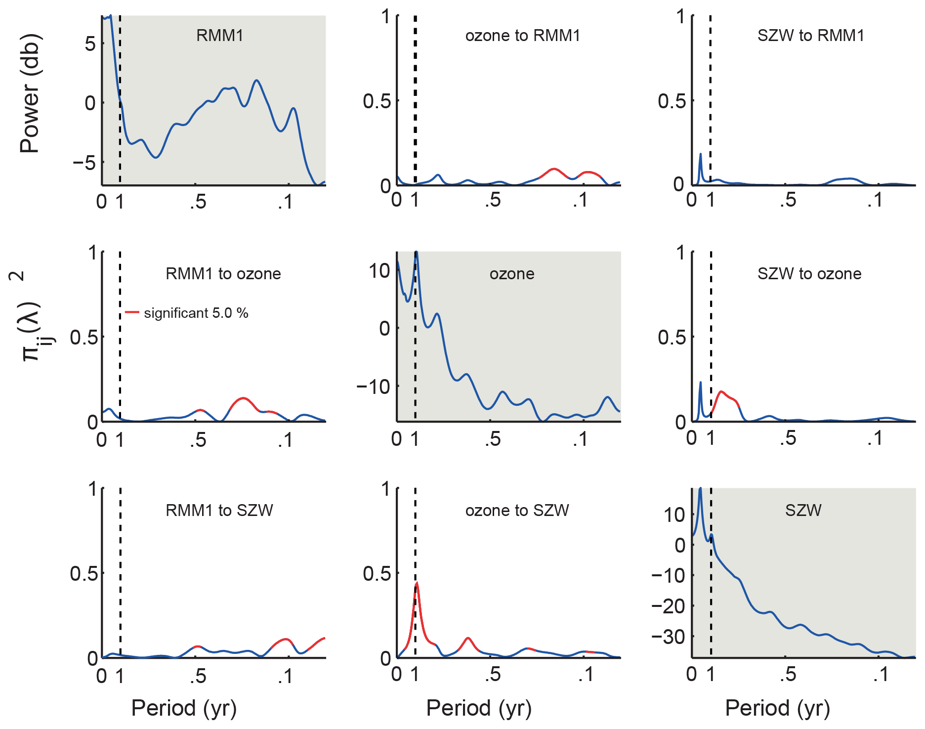
Figure 2PDC between tropical stratospheric ozone and stratospheric zonal wind (SZW) as well as the RMM MJO index at the fast (>20 d) timescale; frequencies are given are given in cycles per year. Panels in the main diagonal show the power spectral density of each time series. Off-diagonal panels indicate the PDC values between the time series. For each panel, the x axis represents the frequency and y axis the value of the PDC. Red lines represent the PDC values that were statistically significant.
From the time series of the amplitudes of the normal-mode functions we compute the energy within a group of modes, consisting of the sum of the squares of their amplitudes weighted by their equivalent depths Dm:
where , and are wavenumber truncations. Throughout the text we select different N to represent different modes (e.g., Kelvin, Rossby, westward inertio-gravity).
Time series of the stratospheric zonal wind at 30 Mb, the equatorial ozone concentration in the stratosphere, and the RMM index are presented in Fig. 1. The autoregressive fitting of the time series was found to be well-represented by passing the Portmanteau test (Lutkepohl, 2005). The PDC analysis for the fast (interannual) timescale, shown in Fig. 2, indicates that there is a statistically significant interaction between the stratospheric mean zonal wind and the MJO and between tropical stratospheric ozone and the MJO; the results here are presented only for RMM1 (RMM2 yields similar results). Concerning the influence of the stratospheric variables on the MJO, tropical stratospheric ozone is shown to have a significant causality (in the Granger sense) on the MJO indices, influencing RMM1 during periods of around 1 month, which corresponds to the higher-frequency range of an MJO cycle. The periods when ozone influences RMM1 and RMM2 show, by the definition of Granger causality, that information on ozone should improve the MJO predictability.
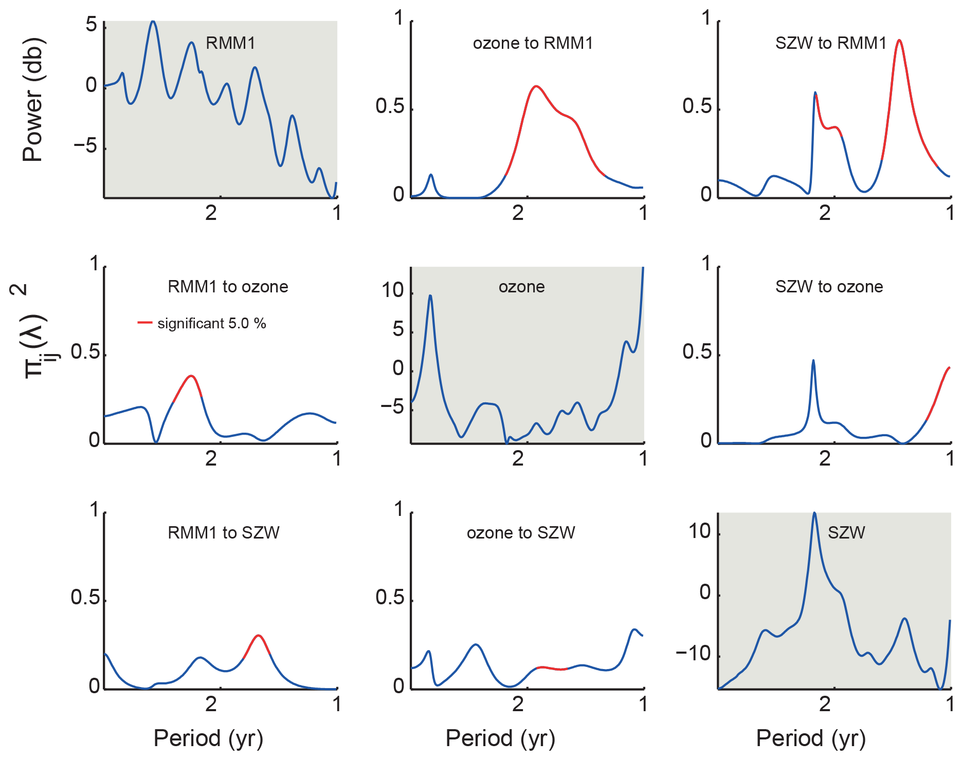
Figure 3PDC analysis between the MJO and stratospheric zonal wind (SZW) at the slow (>1-year periods) timescale. Results indicate significant interaction on annual–biennial timescales. Figure conventions are the same as in Fig. 2.
In order to investigate the interaction between the stratospheric variables and the MJO index we performed a 6-month resampling procedure. Results are presented in Fig. 3. Ozone is found to significantly influence the MJO, as can be seen in Fig. 2, on the annual timescale for RMM2, possibly due to the annual cycle, and on the timescale of 1.6–2.1 years, possibly associated with the QBO. Both RMM indices are found to be significantly affected at frequencies with a peak at 11 years, which is a strong indication of the effect of the solar cycle on the MJO through ozone, which could explain the solar-cycle-related monsoon variability (van Loon and Meehl, 2012); see also Hood (2018) for evidence of the impact of solar variability on the MJO. Interactions that are significant are found from ozone to the MJO in a period ranging from 1 to 2 years, possibly as a combination of the effects of the annual cycle and the QBO, corroborating recent results in the literature (Marshall et al., 2017; Son et al., 2017; Yoo and Son, 2016).
Several studies point to the role of the interaction of waves with different vertical structures in the dynamics of the MJO. For instance, Majda and Biello (2003) studied the interaction of barotropic and baroclinic Rossby waves in the interaction of the tropics and extratropics since barotropic waves are not equatorially confined as baroclinic ones are. Raupp et al. (2008) further explored this mechanism in the initiation of the MJO. A similar mechanism could in principle play a role in stratospheric–tropospheric interactions, with modes with dominant energy in the stratosphere interacting with modes that have more energy in the troposphere. We therefore aim to test such a hypothesis.
We initially perform a linear regression analysis between the time series associated with the MJO indices and the stratospheric zonal wind representative of the QBO, aiming to find which normal modes best represent such oscillations. This analysis was introduced by Žagar et al. (2015) in a normal-mode decomposition of the MJO. Žagar and Franzke (2015) showed that the dominant modes in the decomposition are the symmetric Rossby mode (with the largest contribution coming from the Rossby mode with meridional index 1, denoted by RSSY1) and Kelvin waves (KWs). Both Kelvin and Rossby modes have a larger regression coefficient for the vertical mode indices 5–9, which have a first baroclinic structure in the troposphere. We performed a similar analysis with the daily time series of equatorial zonal wind at 30 hPa, which is dominated by the QBO. We find that the dominant modes in our regression analysis are westward-propagating gravity waves (WIGs) and the first asymmetric Rossby modes (meridional index 2, denoted by RWASY1); we refer to Raphaldini et al. (2020) for details on the normal-mode decomposition of the QBO.
We search for interactions between the MJO and QBO normal modes. In order to do so, we calculate the time series of the energy associated with each of the modes (i.e., a weighted sum of the square of the absolute value of each of the modes). We begin by describing the interaction between modes associated with the MJO and the QBO as well as tropical stratospheric ozone forcing on sub-annual timescales. Due to the large number of variables we split the analysis into three sets, each containing all the “stratospheric variables” against one of the variables associated with the MJO. Since the most important interactions between QBO modes and MJO modes are through the QBO-related WIG waves, we restrict the analysis to these modes.
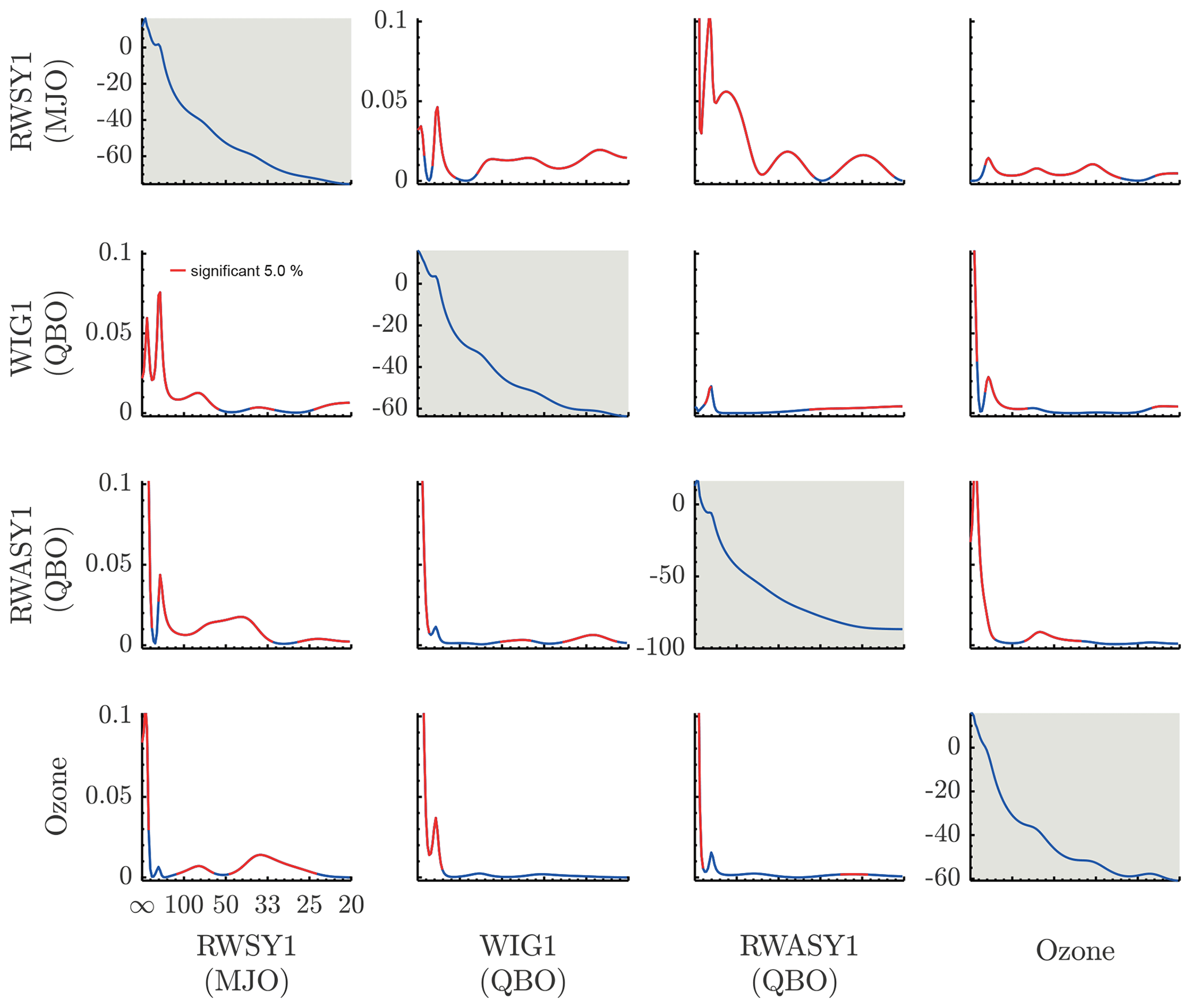
Figure 4PDC analysis of the interaction of Kelvin, asymmetric Rossby, and westward gravity modes with ozone at the fast timescale (periods given in days). Significant interactions (red curve) between the MJO and ozone as well as QBO-related modes are found on intraseasonal, semi-annual, and annual timescales. Panels in the main diagonal show the power spectral density of each time series. Off-diagonal panels indicate the PDC values between the time series; PDC direction is from the time series indicated in the column to the one indicated in the row. For each panel, the x axis represents the frequency and y axis the value of the PDC. Red lines represent the PDC values that were statistically significant.
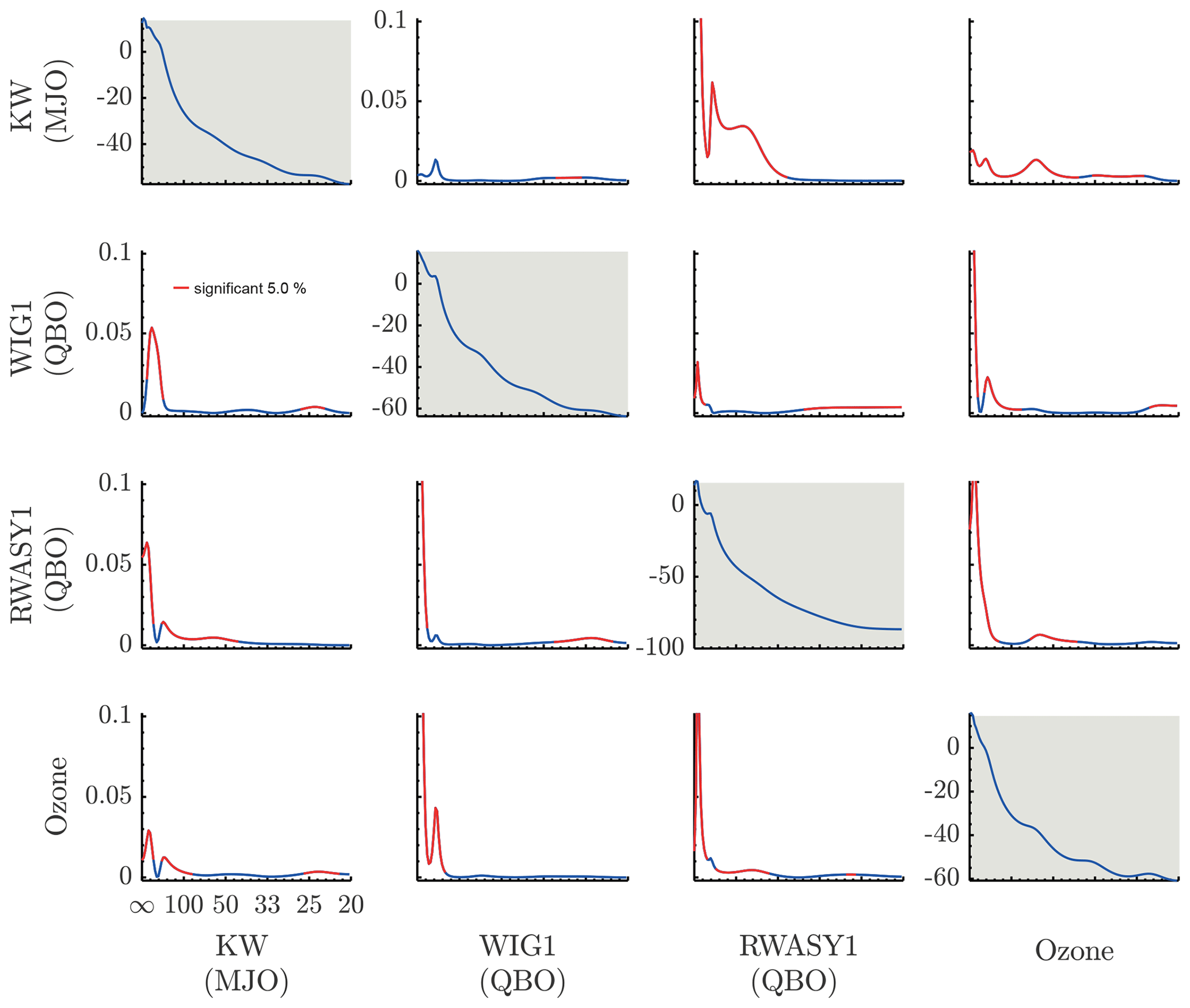
Figure 5PDC analysis of the interaction of symmetric Rossby n=1, asymmetric Rossby n=1, and westward gravity modes with ozone at the fast timescale (periods given in days). Again, significant interactions (red curve) between the MJO and ozone as well as QBO-related modes is found on intraseasonal, semi-annual, and annual timescales. Figure conventions are the same as in Fig. 4.
In Fig. 5 we present the PDC analysis of the interaction of Kelvin waves vs. westward inertio-gravity waves vs. stratospheric ozone vs. asymmetric Rossby waves. The first three variables are associated with stratospheric phenomena and the last one is associated with the MJO. We observe that the ozone forcing acts directly on the MJO-related Kelvin waves, most notably on intraseasonal timescales, with a peak around 50 d. The influence of ozone on this mode is also relevant on a semi-annual and annual timescale, both associated with the annual cycle. WIG waves are found to influence the Kelvin waves on the timescale of 30 d, while asymmetric Rossby waves are found to influence the Kelvin waves on timescales from around 50 d to semi-annual and annual timescales. We find a feedback from Kelvin waves to the stratospheric-related variables on intraseasonal, semi-annual, and annual timescales.
Finally, we perform a PDC analysis of the interaction between symmetric Rossby waves (the dominant mode in the MJO decomposition), asymmetric Rossby waves, WIG waves, and stratospheric ozone on the fast timescale. The corresponding PDC plot is presented in Fig. 4. The influence of stratospheric ozone on symmetric Rossby waves has peaks at 40, 60 d, and on a semi-annual timescale. The influence of the modes associated with the stratospheric zonal wind on the MJO-related Rossby mode seems to be significant throughout the entire intraseasonal timescale range, most notably around 30–40 d, as well as on semi-annual and annual timescales. Similarly to the previous cases, the feedback of the MJO-related mode to the stratospheric-related variables takes place on intraseasonal, semi-annual, and annual timescales.
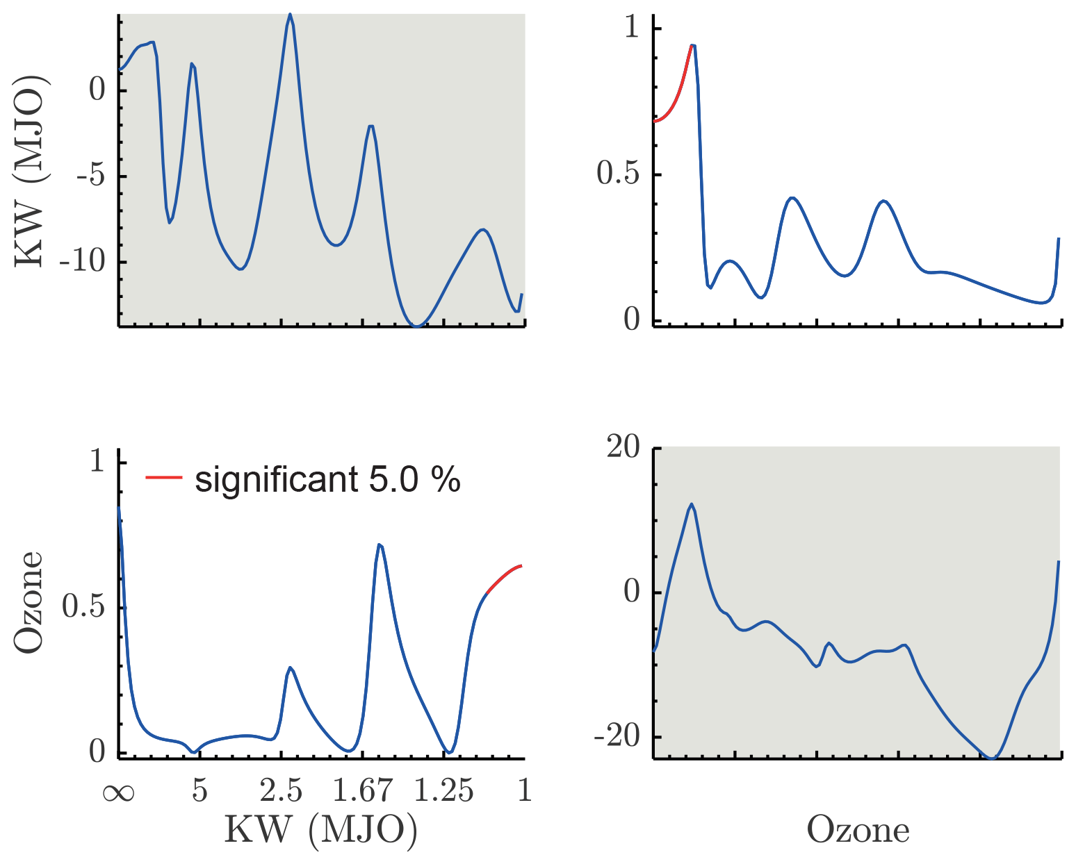
Figure 6PDC analysis of the interaction of ozone modes and Kelvin waves (KWs) at the slow timescale (periods given in years). The results show that KWs influence ozone on the annual timescale, while ozone influences KWs on decadal timescales. Figure conventions are the same as in Fig. 4.
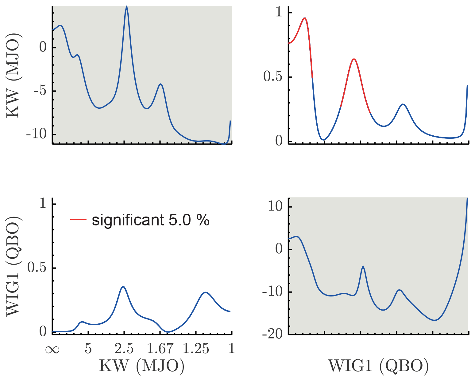
Figure 7PDC analysis of the interaction of Kelvin modes (KWs) and westward gravity modes (WIGs) at the slow timescale (periods given in years). The results show a strong influence of the WIG mode on KWs on biennial and decadal timescales. Figure conventions are the same as in Fig. 4.
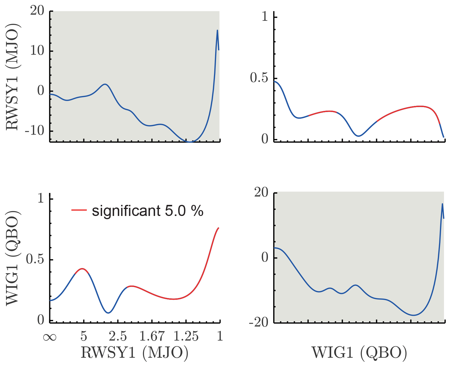
Figure 8PDC analysis of the interaction of symmetric Rossby modes (meridional index 1, denoted by RWSY1) and westward gravity modes (WIG1) at the slow timescale (periods given in years). Important interactions are found on annual to interannual timescales. Figure conventions are the same as in Fig. 4.
We proceed by analyzing the PDC between the modes associated with stratospheric zonal wind and stratospheric ozone vs. MJO-related modes on slow timescales (annual–decadal timescales). Most importantly, we search for stratospheric influences on the MJO on decadal and biennial timescales. The analysis of the interaction between Kelvin waves, associated with the MJO and tropical stratospheric ozone is presented in Fig. 6. It shows that there is a significant causality from ozone to Kelvin waves on a decadal timescale. Given that both spectra have a peak on the decadal timescale we can say that ozone, which is directly influenced by solar variability, has a peak directly associated with the solar cycle, and the peak on the Kelvin wave spectrum is at least partially explained by the influence of ozone on it. Kelvin waves, on the other hand, influence ozone on annual timescales, probably due to the annual cycle. The analysis of the interaction between gravity waves associated with the stratospheric zonal wind and the MJO-related Kelvin waves is presented in Fig. 7. We found an important influence of the westward inertio-gravity waves on the Kelvin waves on biennial timescales and on decadal timescales. The first one is clearly associated with the biennial peak on the inertio-gravity wave spectrum, which is a product of the quasi-biennial oscillation and might be associated with the results of Yoo and Son (2016) and subsequent articles on the relationship between the QBO and the MJO. The PDC peak on the decadal timescale is possibly associated with the solar cycle, and the gravity modes are forced by the ozone (Fig. 9). Since we do not find spectral peaks in this range, we suspect that this is related to the nearest peak, which is annual. A strong causality is also found on a decadal timescale, again probably due to the solar cycle. The influence of WIG modes on the MJO-related Rossby modes is presented in Fig. 8, showing an influence of WIG modes on Rossby modes on annual and biennial timescales.
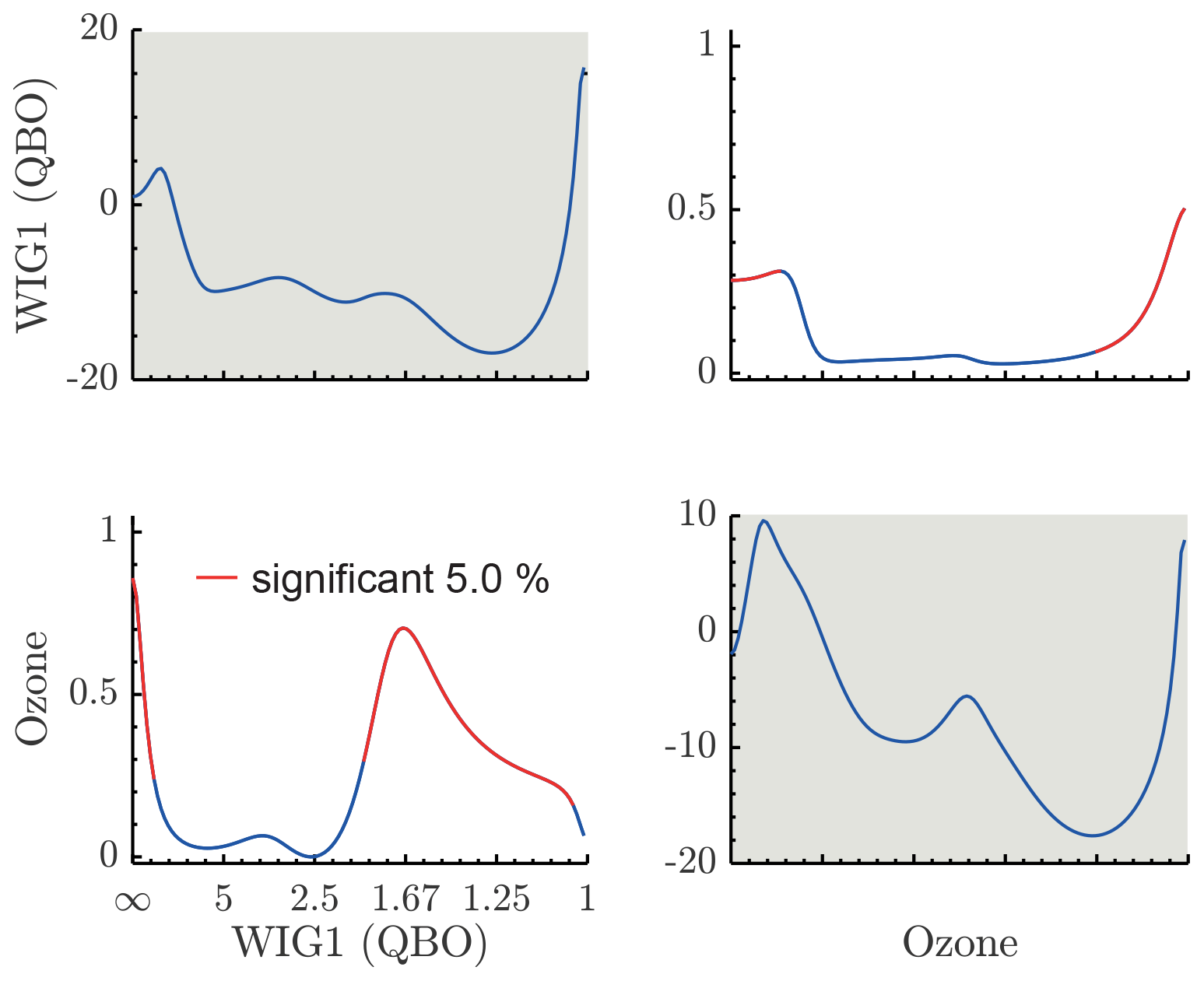
Figure 9PDC analysis of the interaction of westward gravity modes and ozone at the slow timescale (periods given in years). Important interactions are found on annual–biennial timescales and on the decadal timescale. Figure conventions are the same as in Fig. 4.
4.1 Evolution of MJO normal modes
Previous studies point to different MJO behavior depending on the phase of the QBO (east or west) (Yoo and Son, 2016); it is therefore important to examine how and if these differences manifest in the MJO-related normal modes. In order to do so, we follow the methodology used in Franzke et al. (2019) to study the Northern Hemisphere extratropical response of the MJO using normal-mode decomposition. We construct composites representing velocity and pressure fields associated with MJO normal modes for each phase of the MJO. In order to exclude periods without MJO events we include in our analysis only days on which . We then divide the MJO events into eight phases depending on the phase of the MJO for which QBO (positive or negative) state and for which MJO phase () we calculated the mean velocity and pressure fields associated with rotational (ROT) and Kelvin modes at 200 Mb.
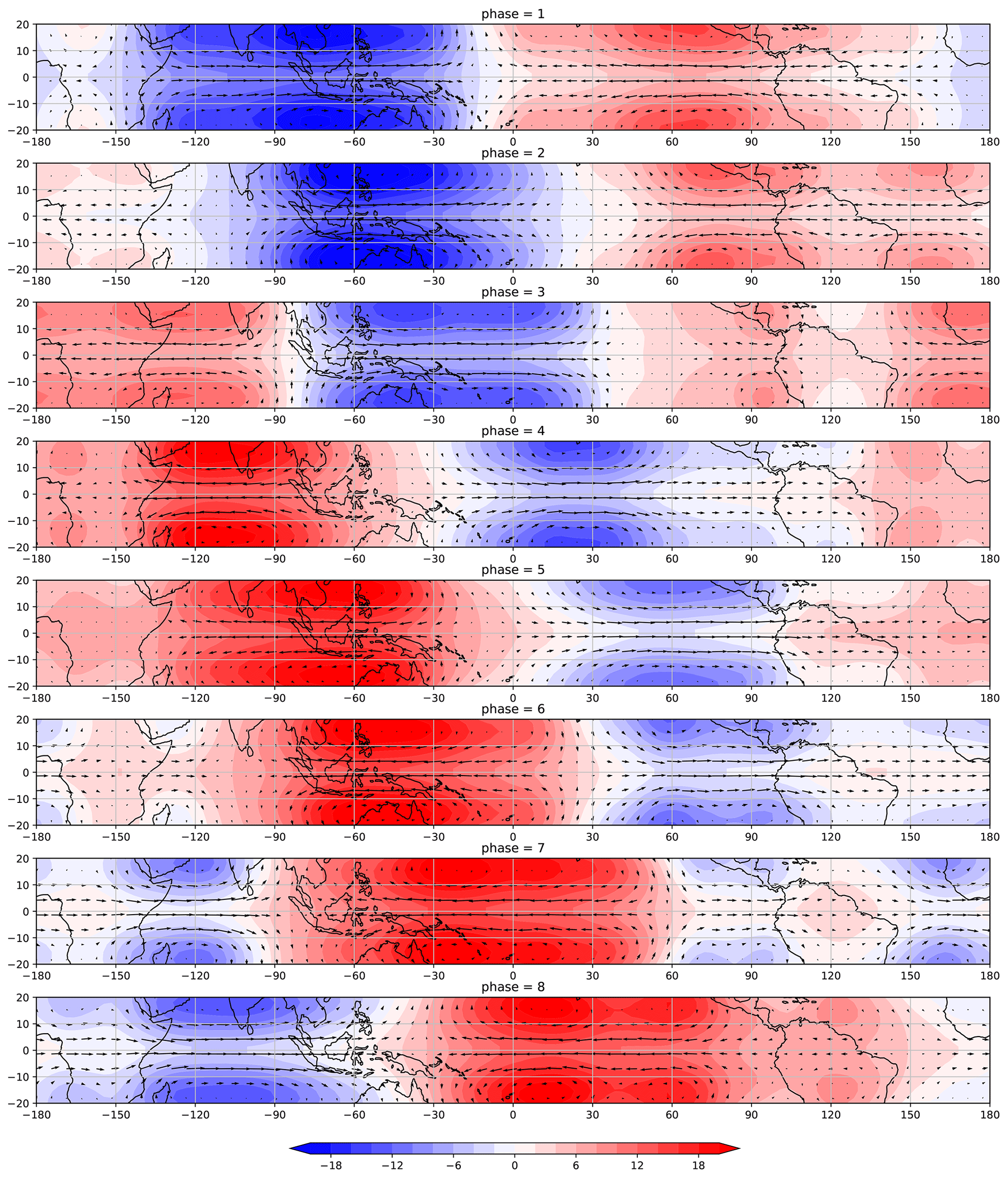
Figure 10Reconstruction at 200 Mb of the velocity and geopotential height fields associated with ROT modes with (positive stratospheric zonal wind) SZW30+.

Figure 11Reconstruction at 200 Mb of the velocity and geopotential height fields associated with ROT modes with (negative stratospheric zonal wind) SZW30−.
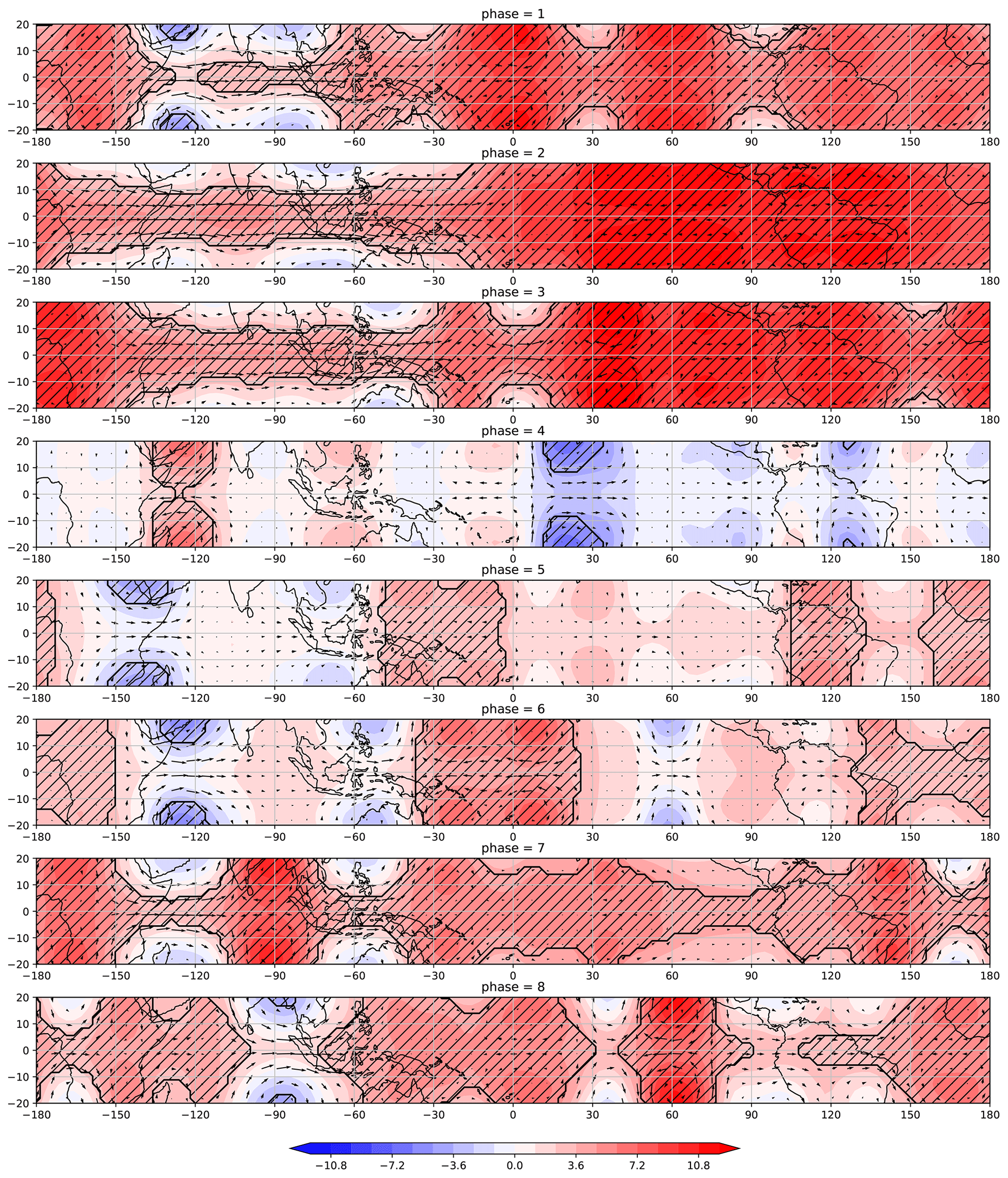
Figure 12Difference between the velocity and geopotential height fields associated with ROT modes with SZW30+ and SZW30−. The hatched region corresponds to a significant difference of the geopotential height values under the 5 % confidence level.
Figures 10 and 11 respectively display the composites associated with the reconstructions of velocity and geopotential height fields associated with ROT modes for each of the eight MJO phases with positive (SZW30+) and negative (SZW30−) stratospheric zonal wind at 30 mb. In order to compare the two composites we compute the difference between SZW30+ and SZW30− of each field for each MJO phase. This is displayed in Fig. 12. We notice that for phases 1–3 the difference (of the geopotential height fields represented by the hatched region) is statistically significant for almost the entire domain. For phase 4 the fields are more similar, with small regions of significant difference associated with Rossby double vortices. Between phases 5 and 8 the areas with significant difference become larger again.
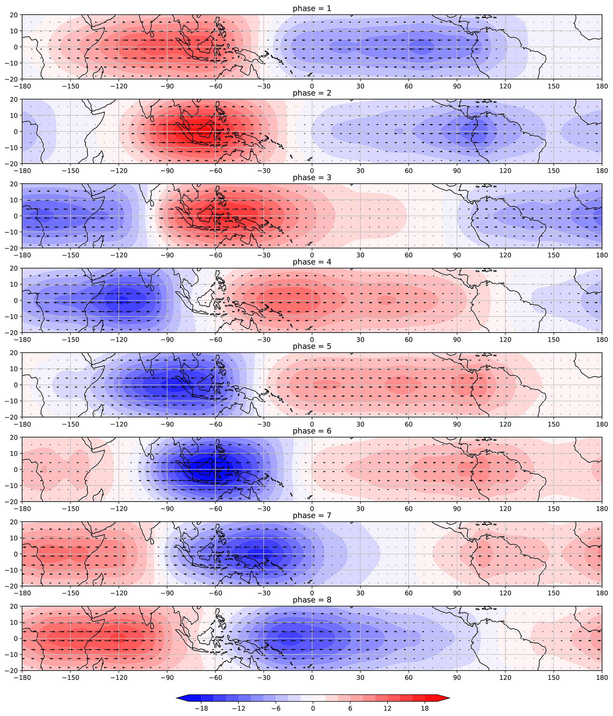
Figure 13Reconstruction at 200 Mb of the velocity and geopotential height fields associated with Kelvin modes with SZW30−.

Figure 14Reconstruction at 200 Mb of the velocity and geopotential height fields associated with Kelvin modes with SZW30−.
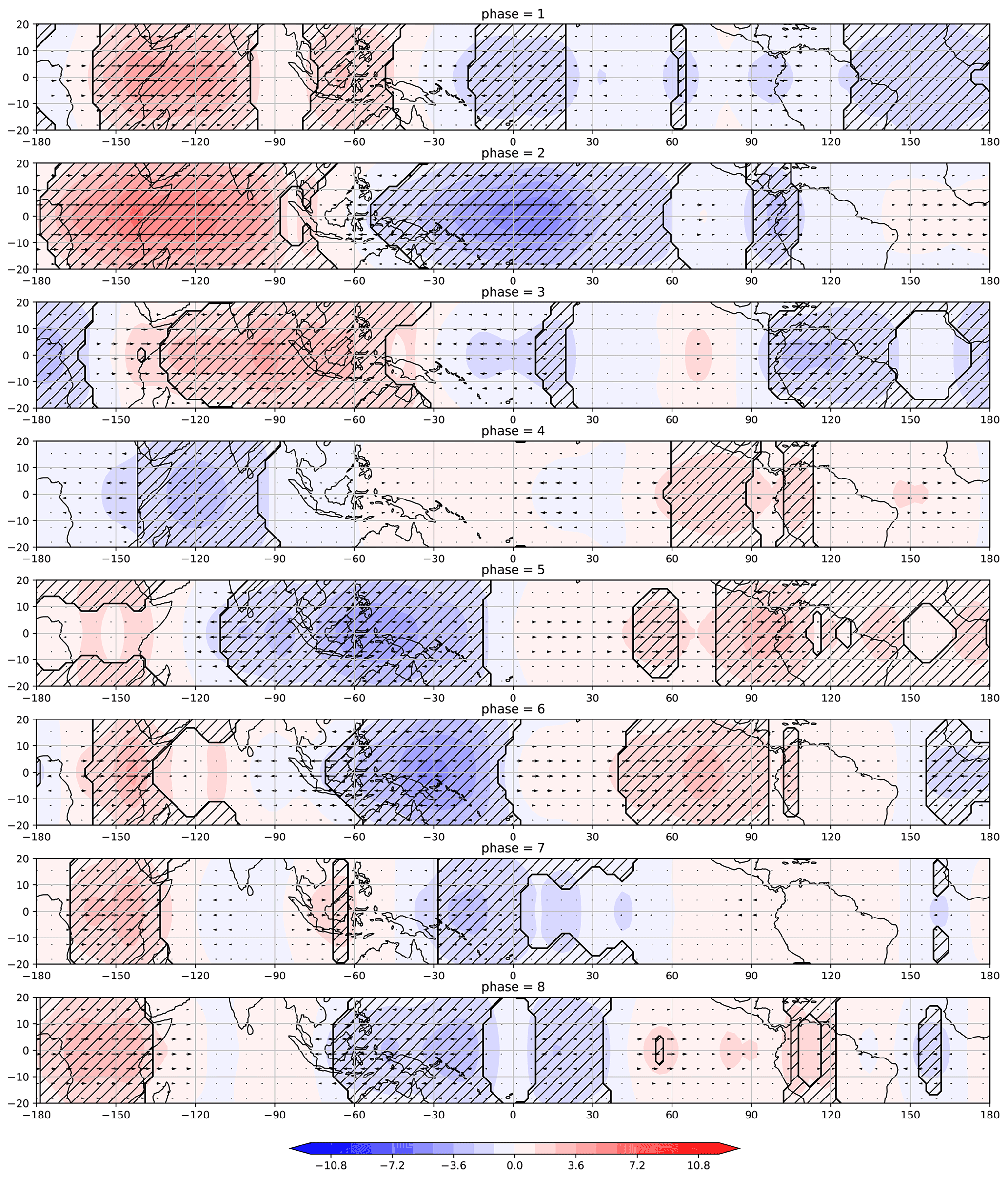
Figure 15Difference between the velocity and geopotential height fields associated with Kelvin modes with SZW30+ and SZW30−. The hatched region corresponds to a significant difference of the geopotential height values under the 5 % confidence level.
Figures 13 and 14 respectively display the composites associated with the reconstructions of velocity and geopotential height fields associated with the Kelvin mode for each of the eight MJO phases with positive (SZW30+) and negative (SZW30−) stratospheric zonal wind at 30 mb. In order to compare the two composites we compute the difference between SZW30+ and SZW30− of each field for each MJO phase. This is displayed in Fig. 15. We notice that for phases 1–3 the difference (of the geopotential height fields represented by the hatched region) is statistically significant for almost the entire domain. Unlike in the case of ROT modes, for the Kelvin modes the distribution of statistically significant difference is more even throughout an MJO cycle, with a larger area in phase 2 and more similar fields in phase 4. It is possible to notice a propagation pattern with a negative geopotential height anomaly beginning in phase 4 and ending in phase 7.
The PDC results show strong coupling between tropical ozone, stratospheric zonal wind, and the MJO. Most notable are the effects of tropical stratospheric winds and ozone influencing the MJO on both intra-annual and interannual timescales. The PDC analysis shows that tropical stratospheric ozone influences the MJO in periods of 30–60 d and 1.5–2.5 years. The first period agrees with the MJO period range, suggesting that stratospheric ozone may play a role in the MJO dynamics. The second roughly agrees with the QBO period, and the third suggests a solar cycle influence on the MJO. Stratospheric zonal winds also influence the MJO during periods that fall into the QBO period range, in agreement with the recent results of Yoo and Son (2016), who showed that there is interannual variability in the MJO amplitude that depends on the QBO phase. Marshall (2016) also shows that the QBO explains up to 40 % of the MJO interannual variability in the boreal winter (see also Son et al., 2017).
By the definition of Granger causality, one signal causes a second signal if the information from the first helps to predict the future of the other after taking into account the past of the second signal. In this sense, we confirm the results of the recent studies cited above. We also show that tropical stratospheric ozone improves MJO predictability on interannual and decadal timescales. The periods of interaction suggest that the QBO might be an important process in troposphere–stratosphere coupling through the MJO. This conclusion agrees with numerical studies such as that of Meehl et al. (2009), stressing the importance of a realistic QBO in coupled troposphere–stratosphere models. We note that ozone influences the MJO on intraseasonal timescales, raising the possibility of tropical stratospheric ozone fluctuations contributing to the initiation of the MJO cycle. On the decadal timescale, ozone and the QBO are modulated by solar activity, and ozone was shown to have important impacts on the MJO on this timescale. There is strong evidence in the literature for a solar cycle impact on the Asian monsoons from both instrumental observations and paleoclimatic reconstructions, with the rainfall rate on the Indian subcontinent increasing by up to 20 % during the solar maximum (van Loon and Meehl, 2012). Since monsoons are linked to the MJO, especially in the Indian region where the MJO signal is strongest, it would be natural to hypothesize that the MJO is a mediator between solar variability and monsoons.
It was also found that the MJO can affect stratospheric ozone, a possible mechanism for this being the impact of deep convection on the tropopause height (Tian et al., 2007). Another interesting question is whether the relationship between the MJO and the QBO is affected by the recent anomalous behavior of the QBO (Osprey et al., 2016; Raphaldini et al., 2020).
As for physical mechanisms that could link stratospheric heating driven by solar UV forcing and tropical convection, tropopause changes caused by ozone absorption are possible candidates. Kang et al. (2011) suggested a polar latitude mechanism associated with changes in wave momentum flux due to ozone depletion associated with the ozone hole. Although this mechanism was proposed for high latitudes, it would be interesting to investigate whether it can be extended to the tropics and to ozone changes due to annual and solar cycles. Recently, Lu et al. (2017) suggested that changes in the waveguides of planetary waves in the stratosphere, caused by solar forcing changes in the mean flow of the stratosphere, might cause downward planetary wave reflection under conditions of high solar activity.
We performed a linear regression analysis of the MJO index and stratospheric zonal winds against the time series of the amplitudes of the Hough modes. We confirm that the MJO is explained mainly by the first symmetric Rossby mode (meridional index 1) and Kelvin modes, in agreement with Žagar and Franzke (2015). The stratospheric zonal wind variability is explained mainly by the WIG modes and the first asymmetric Rossby modes (meridional index 2). We analyzed the interaction among those variables and tropical stratospheric ozone. The exchange of energy between the modes and their interaction with the ozone forcing explain the previous results. We highlight the strong influence of ozone on the MJO-related modes on intraseasonal timescale and on decadal timescales, the last one possibly being a result of the solar cycle. We found the influences of the gravity modes on the MJO-related modes to be the most relevant on biannual timescales. This at least partially explains the work of Yoo and Son (2016) and subsequent articles on the QBO–MJO relation.
A composite analysis of the velocity and geopotential height of the Kelvin and Rossby modes associated with the MJO reveals the differences in the characteristics of these modes during MJO events when the winds are positive at 30 Mb and when they are negative. For the Rossby modes, differences (Fig. 12) are shown to be more significant during the initial (1–3) and final (7–8) phases of an MJO cycle, and the spatial pattern is that expected of the rotational component of the MJO with a double vortex pattern. The differences reveal a stronger rotational component of the MJO when the zonal winds at 30 Mb are positive. For Kelvin modes, significant differences are found throughout the whole MJO cycle, and the composite for the difference between the fields from both QBO phases follows a propagation pattern that seems to evolve eastward with a similar speed as a typical MJO event (5 m s−1). This suggests that the QBO effect on the Kelvin mode is more uniform throughout a QBO cycle, and in the Rossby modes this effect takes place in the initial and final phases of the MJO.
The time series for the amplitudes of the selected normal modes studied here is provided under the following DOI: https://doi.org/10.5281/zenodo.4437766 (Raphaldini et al., 2021).
The supplement related to this article is available online at: https://doi.org/10.5194/esd-12-83-2021-supplement.
BR proposed the study, wrote the paper, and did the statistical analysis. DYT and LM worked on the PDC analysis. AST performed the normal-mode decomposition analysis, and PLdSD helped with the discussion and the interpretation of the analysis.
The authors declare that they have no conflict of interest.
This research was supported by the FAPESP-PACMEDY project (grant nos. 2015/50686-1 and 2017/23417-5), CAPES IAG/USP PROEX (grant no. 0531/2017), and the Meteorology Graduate Program at IAG-USP (CAPES finance code 001).
This paper was edited by Ben Kravitz and reviewed by Christian Franzke and two anonymous referees.
Amos, D. E. and Koopmans, L. H.: Tables of the distribution of the coefficient of coherence for stationary bivariate Gaussian processes, Sandia Corporation, Albuquerque, United States, 1963.
Baccala, L. A. and Sameshima, K.: Overcoming the limitations of correlation analysis for many simultaneously processed neural structures, Prog. Brain Res., 130, 33–47, https://doi.org/10.1016/S0079-6123(01)30004-3, 2001. a, b, c, d
Baccala, L., De Brito, C., Takahashi, D., and Sameshima, K.: Unified asymptotic theory for all partial directed coherence forms, Philos. T. R. Soc. A, 371, 1–13, https://doi.org/10.1098/rsta.2012.0158, 2013. a, b, c, d, e
Baldwin, M. P., Gillett, N. P., Forster, P., Gerber, E. P., Hegglin, M. I., Karpechko, A. Y., Kim, J., Kushner, P. J., Morgenstern, O. H., and Reichler, T.: Effects of the Stratosphere on the Troposphere, chap. 10, in: WMO/ICSU/IOC World Climate Research Programme, Springer, Dordrecht, https://doi.org/10.1007/978-1-4020-8217-7_9, 2010. a
Bianco-Martinez, E. and Baptista, M. S.: Space-time nature of causality, Chaos, 28, 075509, https://doi.org/10.1063/1.5019917, 2018. a
Bressler, S. L. and Seth, A. K.: Wiener–Granger causality: a well established methodology, Neuroimage, 58, 323–329, https://doi.org/10.1016/j.neuroimage.2010.02.059, 2011.
Came, R. E., Oppo, D. W., and McManus, J. F.: Amplitude and timing of temperature and salinity variability in the subpolar North Atlantic over the past 10 ky, Geology, 35, 315–318, https://doi.org/10.1130/G23455A.1, 2007. a
Dee, D. P., Uppala, S. M., Simmons, A. J., Berrisford, P., Poli, P., Kobayashi, S., Andrae, U., Balmaseda, M. A., Balsamo, G., Bauer, P., Bechtold, P., Beljaars, A. C. M., van de Berg, L., Bidlot, J., Bormann, N., Delsol, C., Dragani, R., Fuentes, M., Geer, A. J., Haimberger, L., Healy, S. B., Hersbach, H., Hólm, E. V., Isaksen, L., Kållberg, P., Köhler, M., Matricardi, M., McNally, A. P., Monge‐Sanz, B. M., Morcrette, J.-J., Park, B.-K., Peubey, C., de Rosnay, P., Tavolato, C., Thépaut, J.‐N., and Vitart, F.: The ERA-Interim reanalysis: configuration and performance of the data assimilation system, Q. J. Roy. Meteor. Soc., 137, 553–597, https://doi.org/10.1002/qj.828, 2011. a
Densmore, C. R., Sanabia, E. R., and Barrett, B. S.: QBO influence on MJO amplitude over the Maritime Continent: Physical mechanisms and seasonality, Mon. Weather Rev., 147, 389–406, https://doi.org/10.1175/MWR-D-18-0158.1, 2019. a
Diallo, M., Riese, M., Birner, T., Konopka, P., Müller, R., Hegglin, M. I., Santee, M. L., Baldwin, M., Legras, B., and Ploeger, F.: Response of stratospheric water vapor and ozone to the unusual timing of El Niño and the QBO disruption in 2015–2016, Atmos. Chem. Phys., 18, 13055–13073, https://doi.org/10.5194/acp-18-13055-2018, 2018.
Feldstein, S. B. and Lee, S.: Intraseasonal and Interdecadal Jet Shifts in the Northern Hemisphere: The Role of Warm Pool Tropical Convection and Sea Ice, J. Climate, 27, 6497–6518, https://doi.org/10.1175/JCLI-D-14-00057.1, 2014.
Feng, P. N. and Lin, H.: Modulation of the MJO – related teleconnections by the QBO, J. Geophys. Res.-Atmos., 124, 12022–12033, https://doi.org/10.1029/2019JD030878, 2019. a
Franzke, C. L., Jelic, D., Lee, S., and Feldstein, S. B.: Systematic decomposition of the MJO and its Northern Hemispheric extratropical response into Rossby and inertio-gravity components, Q. J. Roy. Meteor. Soc., 145, 1147–1164, https://doi.org/10.1002/qj.3484, 2019. a
Freitas, A. C. V., Aimola, L., Ambrizzi, T., and de Oliveira, C. P.: Changes in intensity of the regional Hadley cell in Indian Ocean and its impacts on surrounding regions, Meteorol. Atmos. Phys., 43, 1245–1253, https://doi.org/10.1007/s00703-016-0477-6, 2016.
Garfinkel, C. I. and Hartmann, D. L.: The influence of the quasi-biennial oscillation on the troposphere in wintertime in a hierarchy of models. Part I: Simplified dry GCMs, J. Atmos. Sci., 68, 1273–1289, https://doi.org/10.1175/2011JAS3665.1, 2011.
Geweke, J. F.: Measures of conditional linear dependence and feedback between time series, J. Am. Stat. Assoc., 79, 907–915, https://doi.org/10.2307/2288723, 1984.
Granger, C. W. J.: Investigating causal relations by econometric models and cross-spectral methods, Econometrica, 37, 424–438, https://doi.org/10.2307/1912791, 1969. a
Gray, L. J., Beer, J., Geller, M., Haigh, J. D., Lockwood, M., Matthes, K., Cubasch, U., Fleitmann, D., Harrison, G., Hood, L., Luterbacher, J., Meehl, G. A., Shindell, D., Van Geel, B., and White, W.: Solar influence on climate, Rev. Geophys., 48, RG4001, https://doi.org/10.1029/2009RG000282, 2010. a
Haigh, J. D. and Blackburn, M.: Solar influences on dynamical coupling between the stratosphere and troposphere, Space Sci. Rev., 125, 331–344, https://doi.org/10.1007/s11214-006-9067-0, 2006.
Hendon, H. H. and Abhik, S.: Differences in Vertical Structure of the Madden–Julian Oscillation Associated With the Quasi–Biennial Oscillation, Geophys. Res. Lett., 45, 4419–4428, https://doi.org/10.1029/2018GL077207, 2018. a, b
Holton, J. R. and Tan, H. C.: The influence of the equatorial quasi-biennial oscillation on the global circulation at 50 mb, J. Atmos. Sci., 37, 2200–2208, https://doi.org/10.1175/1520-0469(1980)037<2200:TIOTEQ>2.0.CO;2, 1980. a
Hood, L. L.: Short-term solar modulation of the Madden–Julian climate oscillation, J. Atmos. Sci., 75, 857–873, https://doi.org/10.1175/JAS-D-17-0265.1, 2018. a
Hui, E. C. and Chen, J.: Investigating the change of causality in emerging property markets during the financial tsunami, Physica A, 391, 3951–3962, https://doi.org/10.1016/j.physa.2012.03.007, 2012. a
Huybers, P. and Curry, W.: Links between annual, Milankovitch and continuum temperature variability, Nature, 441, 329–332, https://doi.org/10.1038/nature04745, 2006. a
Kang, S. M., Polvani, L. M., Fyfe, J. C., and Sigmond, M.: Impact of Polar Ozone Depletion on Subtropical Precipitation, Science, 332, 951, https://doi.org/10.1126/science.1202131, 2011. a
Kasahara, A. and Puri, K.: Spectral representation of three-dimensional global data by expansion in normal mode functions, Mon. Weather Rev., 109, 37–51, https://doi.org/10.1175/1520-0493(1981)109<0037:SROTDG>2.0.CO;2, 1981. a
Khouider, B., Majda, A. J., and Stechmann, S. N.: Climate science in the tropics: waves, vortices and PDEs, Nonlinearity, 26, R1, https://doi.org/10.1088/0951-7715/26/1/R1, 2012. a
Kidston, J., Scaife, A. A., Hardiman, S. C., Mitchell, D. M., Butchart, N., Baldwin, M. P., and Gray, L. J.: Stratospheric influence on tropospheric jet streams, storm tracks and surface weather, Nat. Geosci., 8, 433–440, https://doi.org/10.1038/ngeo2424, 2015. a
Kim, H., Caron, J. M., Richter, J. H., and Simpson, I. R.: The lack of QBO-MJO connection in CMIP6 models, Geophys. Res. Lett., 47, e2020GL087295, https://doi.org/10.1029/2020GL087295, 2020. a
Kitsios, V., O'Kane, T. J., and Žagar, N.: A Reduced-Order Representation of the Madden–Julian Oscillation Based on Reanalyzed Normal Mode Coherences, J. Atmos. Sci., 76, 2463–2480, https://doi.org/10.1175/JAS-D-18-0197.1, 2019. a
Kretschmer, M., Cohen, J., Matthias, V., Runge, J., and Coumou, D.: The different stratospheric influence on cold-extremes in Eurasia and North America, npj Clim. Atmos. Sci., 1, 44, https://doi.org/10.1038/s41612-018-0054-4, 2018.
Li, K.-F., Tian, B., Waliser, D. E., Schwartz, M. J., Neu, J. L., Worden, J. R., and Yung, Y. L.: Vertical structure of MJO-related subtropical ozone variations from MLS, TES, and SHADOZ data, Atmos. Chem. Phys., 12, 425–436, https://doi.org/10.5194/acp-12-425-2012, 2012.
Liu, Y., Wang, L., and Zhou, W.: Three Eurasian teleconnection patterns: Spatial structures, temporal variability, and associated winter climate anomalies, Clim. Dynam., 42, 2817–2839, https://doi.org/10.1007/s00382-014-2163-z, 2014.
Longuet-Higgins, M. S.: The eigenfunctions of Laplace's tidal equation over a sphere, Philos. T. Roy. Soc. A, 262, 511–607, https://doi.org/10.1098/rsta.1968.0003, 1968. a
Lu, H., Scaife, A. A., Marshall, G. J., Turner, J., and Gray, L. J.: Downward Wave Reflection as a Mechanism for the Stratosphere–Troposphere Response to the 11-Yr Solar Cycle, J. Climate, 30, 2395–2414, https://doi.org/10.1175/JCLI-D-16-0400.1, 2017. a, b
Lutkepohl, H.: New Introduction to Multiple Time Series Analysis, Springer, Berlin, https://doi.org/10.1007/978-3-540-27752-1, 2005. a, b
Majda, A. J. and Biello, J. A.: The nonlinear interaction of barotropic and equatorial baroclinic Rossby waves, J. Atmos. Sci., 60, 1809–1821, https://doi.org/10.1175/1520-0469(2003)060<1809:TNIOBA>2.0.CO;2, 2003. a
Massaroppe, L. and Baccala, L. A.: Detecting nonlinear Granger causality via the kernelization of partial directed coherence, ISI-International Statistical Institute, Rio de Janeiro, RJ, 2015a. a
Massaroppe, L. and Baccala, L. A.: Kernel-nonlinear-PDC extends Partial Directed Coherence to detecting nonlinear causal coupling, in: 2015 37th Annual International Conference of the IEEE Engineering in Medicine and Biology Society (EMBC), 25–29 August 2015, Milan, Italy, IEEE, 2864–2867, https://doi.org/10.1109/EMBC.2015.7318989, 2015b.
Marshall, A. G., Hedon, H. H., Son, S.-W., and Lim, Y.: Impact of the quasi-biennial oscillation on predictability of the Madden–Julian oscillation, Clim. Dynam., 49, 1365–1377, https://doi.org/10.1007/s00382-016-3392-0, 2016. a, b
Meehl, G. A., Arblaster, J. M., Matthes, K., Sassi, F., and van Loon, H.: Amplifying the Pacific climate system response to a small 11-year solar cycle forcing, Science, 325, 1114–1118, https://doi.org/10.1126/science.1172872, 2009. a
Monster, D., Fusaroli, R., Tylén, K., Roepstorff, A., and Sherson, J. F.: Causal inference from noisy time-series data – Testing the Convergent Cross-Mapping algorithm in the presence of noise and external influence, Future Gener. Comp. Sy., 73, 52–62, https://doi.org/10.1016/j.future.2016.12.009, 2017. a
Nappo, C. J.: An introduction to atmospheric gravity waves, Academic Press, Knoxville, Tennessee, USA, ISBN: 978-0-12-514082-9, 2013. a
Nishimoto, E. and Yoden, S.: Influence of the stratospheric quasi-biennial oscillation on the Madden–Julian oscillation during austral summer, J. Atmos. Sci., 74, 1105–1125, https://doi.org/10.1175/JAS-D-16-0205.1, 2017. a
Osprey, S. M., Butchart, N., Knight, J. R., Scaife, A. A., Hamilton, K., Anstey, J. A., Schenzinger, V., and Zhang, C.: An unexpected disruption of the atmospheric quasi-biennial oscillation, Science, 353, 6306, 1424–1427, https://doi.org/10.1126/science.aah4156, 2016. a
Percival, D. B. and Walden, A. T.: Spectral Analysis for Physical Applications: Multitaper and Conventional Univariate Techniques, Cambridge University Press, Cambridge, https://doi.org/10.1017/CBO9780511622762, 1993.
Raphaldini, B., Wakate Teruya, A. S., Silva Dias, P. L., Chavez Mayta, V. R., and Takara, V. J.: Normal mode perspective on the 2016 QBO disruption: Evidence for a basic state regime transition, Geophys. Res. Lett., 47, e2020GL087274. https://doi.org/10.1029/2020GL087274, 2020. a, b, c
Raphaldini, B., Teruya, A. S., Dias, P. L. S., Takahashi, D. Y., and Massaroppe, L.: Stratospheric Ozone and Quasi-Biennial Oscillation (QBO) interaction with the tropical troposphere on intraseasonal and interannual timescales: a normal-mode perspective, Zenodo, https://doi.org/10.5281/zenodo.4437766, 2021. a
Raupp, C. F., Silva Dias, P. L., Tabak, E. G., and Milewski, P.: Resonant wave interactions in the equatorial waveguide, J. Atmos. Sci., 65, 3398–3418, https://doi.org/10.1175/2008JAS2387.1, 2008. a
Schelter, B., Winterhalder, M., Eichler, M., Peifer, M., Hellwig, B., Guschlbauer, B., and Timmer, J.: Testing for directed influences among neural signals using partial directed coherence, J. Neurosci. Meth., 152, 210–219, https://doi.org/10.1016/j.jneumeth.2005.09.001, 2006. a
Sameshima, K. and Baccalá, L. A.: Using partial directed coherence to describe neuronal ensemble interactions, J. Neurosci. Meth., 94, 93–103, https://doi.org/10.1016/S0165-0270(99)00128-4, 1999.
Sameshima, K., Takahashi, D. Y., and Baccalá, L. A.: On the statistical performance of Granger-causal connectivity estimators, Brain Inf., 2, 119–133, https://doi.org/10.1007/s40708-015-0015-1, 2015. a, b
Sato, J. R., Takahashi, D. Y., Arcuri, S. M., Sameshima, K., Morettin, P. A., and Baccalá, L. A.: Frequency domain connectivity identification: an application of partial directed coherence in fMRI, Hum. Brain Mapp., 30, 452–461, https://doi.org/10.1002/hbm.20513, 2009. a
Serfling, R. J.: Approximation Theorems of Mathematical Statistics, John Wiley and Sons, New York, https://doi.org/10.1002/9780470316481, 1980. a
Singh, S. V., Kripalani, R. H., and Sikka, D. R.: Interannual variability of the Madden-Julian oscillations in Indian summer monsoon rainfall, J. Climate, 5, 973–978, https://doi.org/10.1175/1520-0442(1992)005<0973:IVOTMJ>2.0.CO;2, 1992.
Sugihara, G., May, R., Ye, H., Hsieh, C. H., Deyle, E., Fogarty, M., and Munch, S.: Detecting causality in complex ecosystems, Science, 338, 496–500, https://doi.org/10.1126/science.1227079, 2012. a, b
Son, S.-W., Lim, Y., Yoo, C., Hendon, H. H., and Kim, J.: Stratospheric control of Madden-Julian Oscillation, J. Climate, 30, 1909–1922, https://doi.org/10.1175/JCLI-D-16-0620.1, 2017. a, b, c
Takahashi, D. Y., Baccala, L. A., and Sameshima, K.: Connectivity inference between neural structures via partial directed coherence, J. Appl. Stat., 10, 1259–1273, https://doi.org/10.1080/02664760701593065, 2007. a, b, c, d
Takahashi, D. Y., Baccalá, L. A., and Sameshima, K.: Information theoretic interpretation of frequency domain connectivity measures, Biol. Cybern., 103, 463–469, https://doi.org/10.1007/s00422-010-0410-x, 2010. a, b, c, d
Tirabassi, G., Sommerlade, L., and Masoller, C.: Inferring directed climatic interactions with renormalized partial directed coherence and directed partial correlation, Chaos, 27, 035815, https://doi.org/10.1063/1.4978548, 2017.
Tian, B., Yung, Y., Waliser, D., Tyranowski, T., Kuai, L., Fetzer, E., and Irion, F.: Intraseasonal variations of the tropical total ozone and their connection to the Madden-Julian Oscillation, Geophys. Res. Lett., 34, L08704, https://doi.org/10.1029/2007GL029451, 2007. a
Tirabassi, G., Sommerlade, L., and Masoller, C.: Inferring directed climatic interactions with renormalized partial directed coherence and directed partial correlation, Chaos, 27, 035815, https://doi.org/10.1029/2012GL051977, 2017. a
van Loon, H. and Meehl, G. A.: The Indian summer monsoon during peaks in the 11 year sunspot cycle, Geophys. Res. Lett., 39, L13701, https://doi.org/10.1029/2012GL051977, 2012. a, b
Wahl, B., Feudel, U., Hlinka, J., Wächter, M., Peinke, J., and Freund, J. A.: Granger-causality maps of diffusion processes, Phys. Rev. E, 93, 022213, https://doi.org/10.1103/PhysRevE.93.022213, 2016. a
Wheeler, M. C. and Hendon, H. H.: An All-Season Real-Time Multivariate MJO Index: Development of an Index for Monitoring and Prediction, Mon. Weather Rev., 132, 1917–1932, https://doi.org/10.1175/1520-0493(2004)132<1917:AARMMI>2.0.CO;2, 2004. a
Winterhalder, M., Schelter, B., and Timmer, J.: Detecting coupling directions in multivariate oscillatory systems, Int J Bifurcat. Chaos, 17, 3735–3739, https://doi.org/10.1142/S0218127407019664, 2007. a
Yoo, C. and Son, S.-W.: Modulation of the boreal winter time Madden-Julian oscillation by thestratospheric quasi-biennial oscillation, Geophys. Res. Lett., 43, 1392–1398, https://doi.org/10.1002/2016GL067762, 2016. a, b, c, d, e, f, g
Žagar, N. and Franzke, C. L.: Systematic decomposition of the Madden–Julian Oscillation into balanced and inertio-gravity components, Geophys. Res. Lett., 42, 6829–6835, https://doi.org/10.1002/2015GL065130, 2015. a, b, c, d
Žagar, N., Kasahara, A., Terasaki, K., Tribbia, J., and Tanaka, H.: Normal-mode function representation of global 3-D data sets: open-access software for the atmospheric research community, Geosci. Model Dev., 8, 1169–1195, https://doi.org/10.5194/gmd-8-1169-2015, 2015. a, b, c, d
Zhang, C.: Madden–julian oscillation, Rev. Geophys., 43, RG2003, https://doi.org/10.1029/2004RG000158, 2005. a
Zhang, C. and Zhang, B.: QBO-MJO Connection, J. Geophys. Res.-Atmos., 123, 2957–2967, https://doi.org/10.1002/2017JD028171, 2018. a
Zhang, T., Wang, T., Krinner, G., Wang, X., Gasser, T., Peng, S., Piao, S., and Yao, T.: The weakening relationship between Eurasian spring snow cover and Indian summer monsoon rainfall, Sci. Adv., 5, eaau8932, https://doi.org/10.1126/sciadv.aau8932, 2019.