the Creative Commons Attribution 4.0 License.
the Creative Commons Attribution 4.0 License.
 | 30 Jun 2021
Comparison of uncertainties in land-use change fluxes from bookkeeping model parameterisation
Kerstin Hartung
Tobias B. Nützel
Julia E. M. S. Nabel
Richard A. Houghton
Julia Pongratz
Fluxes from deforestation, changes in land cover, land use and management practices (FLUC for simplicity) contributed to approximately 14 % of anthropogenic CO2 emissions in 2009–2018. Estimating FLUC accurately in space and in time remains, however, challenging, due to multiple sources of uncertainty in the calculation of these fluxes. This uncertainty, in turn, is propagated to global and regional carbon budget estimates, hindering the compilation of a consistent carbon budget and preventing us from constraining other terms, such as the natural land sink. Uncertainties in FLUC estimates arise from many different sources, including differences in model structure (e.g. process based vs. bookkeeping) and model parameterisation. Quantifying the uncertainties from each source requires controlled simulations to separate their effects.
Here, we analyse differences between the two bookkeeping models used regularly in the global carbon budget estimates since 2017: the model by Hansis et al. (2015) (BLUE) and that by Houghton and Nassikas (2017) (HN2017). The two models have a very similar structure and philosophy, but differ significantly both with respect to FLUC intensity and spatiotemporal variability. This is due to differences in the land-use forcing but also in the model parameterisation.
We find that the larger emissions in BLUE compared to HN2017 are largely due to differences in C densities between natural and managed vegetation or primary and secondary vegetation, and higher allocation of cleared and harvested material to fast turnover pools in BLUE than in HN2017. Besides parameterisation and the use of different forcing, other model assumptions cause differences: in particular that BLUE represents gross transitions which leads to overall higher carbon losses that are also more quickly realised than HN2017.
Please read the corrigendum first before continuing.
-
Notice on corrigendum
The requested paper has a corresponding corrigendum published. Please read the corrigendum first before downloading the article.
-
Article
(4009 KB)
- Corrigendum
- Companion paper
-
Supplement
(168 KB)
-
The requested paper has a corresponding corrigendum published. Please read the corrigendum first before downloading the article.
- Article
(4009 KB) - Full-text XML
- Corrigendum
- Companion paper
-
Supplement
(168 KB) - BibTeX
- EndNote


Changes in land use and management are estimated to have contributed to a global source of CO2 to the atmosphere from the pre-industrial period until the present, and to account for more than 10 % of the total CO2 emissions over the past decade according to the Global Carbon Budget 2019 (Friedlingstein et al., 2019). Fluxes from land-use change and management (FLUC) result from changes in vegetation and soil carbon stocks and product pools due to human activities, such as deforestation, forest degradation, afforestation and reforestation, as well as management practices such as wood harvest and shifting cultivation (rotation cycle between forest and agriculture), and subsequent regrowth of natural vegetation following harvest or agricultural abandonment.
Reconstructing these changes consistently over the globe for the past centuries (let alone millennia) is, however, challenging and associated with high uncertainties (Hurtt et al., 2020; Klein Goldewijk et al., 2017; Pongratz et al., 2014; Ramankutty and Foley, 1999). This uncertainty in forcing translates directly to uncertainties in FLUC estimates (Gasser et al., 2020; Pongratz et al., 2009; Stocker et al., 2011). Moreover, differences in definitions and terminology, and on how indirect environmental effects such as increasing atmospheric CO2 concentration are considered lead to large differences in FLUC estimated by different methods (Gasser and Ciais, 2013; Grassi et al., 2018; Pongratz et al., 2014; Stocker and Joos, 2015). Grassi et al. (2018) have shown that by harmonising definitions of managed land, estimates of FLUC by a bookkeeping (BK) model, dynamic global vegetation models (DGVMs) and national inventories can be in part reconciled. The indirect environmental effects (accounted for in DGVMs but not in BK models) can be calculated by factorial simulations, in order to compare estimates from these two methods (Bastos et al., 2020). Whether and how these indirect effects are accounted for in FLUC creates large differences between estimates but can be resolved by a consistent terminology (Grassi et al., 2018; Pongratz et al., 2014). Besides uncertainty in historical land-use change (LUC) areas and terminological issues, studies also differ with respect to which LUC practices are considered. Several studies have shown that including management practices such as shifting cultivation, crop or wood harvesting might increase FLUC by 70 % or more in individual DGVM estimates (Arneth et al., 2017; Pugh et al., 2015) with management processes explaining some of the differences between biospheric fluxes from DGVMs and top-down estimates (Bastos et al., 2020).
In the global carbon budgets since 2017 (Friedlingstein et al., 2019; Le Quéré et al., 2018a, b), FLUC estimates for recent decades are taken as the mean of the estimates of two BK models, the one from Houghton and Nassikas (2017) (HN2017) and the BLUE model described in Hansis et al. (2015). However, even for these similar methods, estimates differ considerably (Bastos et al., 2020; Friedlingstein et al., 2019). Cumulative FLUC from 1850 until the present day by these two BK models is 205±60 PgC in the Global Carbon Budget 2019 (Friedlingstein et al., 2019; GCB2019 in the following). The FLUC uncertainty after 1959 has been defined by best value judgement that there is a 68 % likelihood that actual FLUC lies within ±0.7 PgC yr−1 of the two models' mean, and for earlier periods, the standard deviation of a group of DGVMs was used. This uncertainty range reflects uncertainties in parameterisations of the BK models, in the applied land-use change forcings as well as definitions, processes considered, and is large enough to encompass the two models' estimates.
Besides differences in cumulative FLUC, BLUE and HN2017 also show very different temporal behaviours (Friedlingstein et al., 2019, and see Fig. 2 below). Noteworthy is an increase in FLUC in BLUE but decrease in HN2017 in the 1950s, which is likely attributable to the change in methodology in HYDE (Klein Goldewijk et al., 2017) from using FAOSTAT (FAOSTAT, 2015) estimates to population-based extrapolation in the past (Bastos et al., 2016). This comes on top of a generally steeper increase in FLUC in BLUE in 1870–1950. A second notable difference in temporal dynamics can be observed in the 2000s, as has been shown by Bastos et al. (2020). Here, BLUE shows a strong increasing trend starting 2000, while HN2017 estimates start decreasing after the late 1990s.
The estimated uncertainty of FLUC in the global carbon budgets is thus approximately 0.7 PgC yr−1 or approximately ±50 % of the average value, substantially larger than that of fossil fuel emissions. This uncertainty, in turn, is propagated to global and regional carbon budget estimates and affects the land sink term, which has often been quantified as residual depending on FLUC. Houghton (2020) further noted that while net FLUC can be constrained by the global carbon budgets, the component gross fluxes (sources such as deforestation and sinks, e.g. by afforestation) are even more uncertain.
Differences in initial land-cover distribution and transitions across different forcing datasets can also lead to substantial differences in estimated FLUC (Di Vittorio et al., 2020; Li et al., 2018; Gasser et al., 2020). A detailed analysis of the impact of the forcing datasets on LUC estimated by the OSCAR bookkeeping (BK) model has been performed by Gasser et al. (2020), and Hartung et al. (2021) analysed the effect of the different LUC from the Land-Use Harmonization dataset (LUH2v2.1) (Hurtt et al., 2020) and of various internal model assumptions in BLUE on FLUC.
Despite the relevance of the BLUE and HN2017 estimates for the global carbon budget analyses, stark discrepancies between these two models (Friedlingstein et al., 2019) and the long-standing appreciation of various factors contributing to such differences (Hansis et al., 2015; Houghton et al., 2012), no quantitative analysis on the contribution of model differences to this discrepancy has so far been performed. Both models rely on observation-based estimates for their parameterisations and forcing datasets, and the choices on spatial and plant functional type representation, starting year and other aspects are well justified in both models. However, these multiple differences add to uncertainty in FLUC estimates and make it difficult to attribute differences in FLUC and their trends to specific aspects of the FLUC calculation.
In this study, we fill this gap and assess to which extent the different parameterisations in BLUE and HN2017 affect global and regional FLUC estimates and their trends. We further investigate the effect of the different parameter choices on the gross LUC fluxes.
2.1 Model characteristics and datasets used
In this study, we focus on the two BK models used in the GBC2019 as well as in the Intergovernmental Panel on Climate Change's Special Report on Climate Change and Land (IPCC, 2019) to estimate FLUC: the Bookkeeping of Land-Use change Emissions model, BLUE (Hansis et al., 2015) and the model from Houghton and Nassikas (2017), which is referred to as HN2017.
The two models differ in several aspects, the most relevant ones summarised in Table 1. An important difference, which we will account for in this study, is that BLUE estimates FLUC from gross LUC transitions, while HN2017 uses net transitions. Gross transitions resolve that within a unit (grid cell for BLUE, country/region for HN2017) there may be concurrent back-and-forth transitions between a pair of land-use types; for example, 30 % of the unit area may be transformed from forest to cropland, while on 20 % cropland is abandoned and forest regrows. Net transitions would represent this as a 10 % forest to cropland transition. These sub-unit changes are particularly important for large units (large grid cells or country level; Wilkenskjeld et al., 2014) and in regions where shifting cultivation prevails (in particular in the tropics; Heinimann et al., 2017) or with small-scale dynamics such as in Europe (Fuchs et al., 2015). HN2017 implicitly includes shifting-cultivation effects if these are captured by FAO (2015) data and allows degraded lands start to accumulate carbon again after 10 years of no change. The two models are also forced by distinct LUC datasets: HN2017 calculated FLUC at country level based on statistics of changes in croplands and pastures extent since 1961 and harvest data and changes in forests and other land since 1990 (FAO, 2015; FAOSTAT, 2015), with extrapolations to earlier time periods. BLUE, on the other hand, is forced by spatially explicit transitions and harvest at 0.25×0.25∘ resolution from LUH2v2.1 (Friedlingstein et al., 2019; Hurtt et al., 2020). LUH2v2.1 calculates cropland, pasture, urban and ice/water fractions between 850 and 2018 based on the HYDE3.1 dataset (Klein Goldewijk et al., 2017). HYDE3.1 in turn, also used FAOSTAT (2015) data for country-level agricultural areas (cropland, pasture, rangelands) data after 1961, extrapolated backwards in time using total population and agricultural area per-capita ratios for each country. The cropland and forest area estimates from these two different datasets (LUH2v2.1 vs. FAO) differ considerably in several key LUC areas, for example, South America and SE Asia (Li et al., 2018), which can lead to large differences in FLUC and their trends found in those regions (Bastos et al., 2020; Di Vittorio et al., 2020).
Table 1Summary of the most important characteristics of the two FLUC estimates from the two BK models used in the GCB2019 (BLUE and HN2017), including how FLUC is calculated in the standard version and configuration of each model, the processes represented and how they are parameterised. The model assumptions and parameterisations investigated in this study (see Table 2) are highlighted in bold.
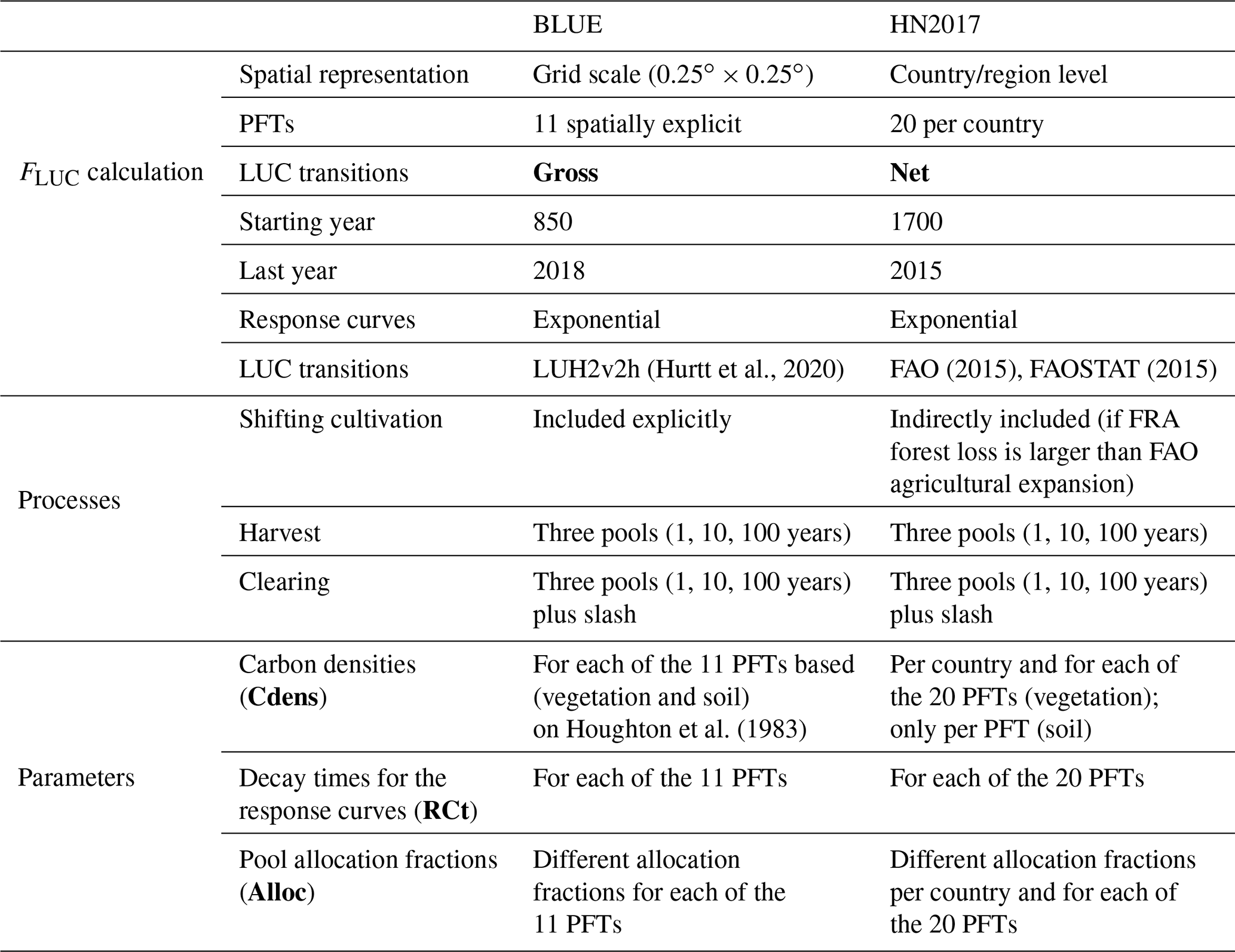
Following a transition, C stocks in the different pools will decay following response curves with characteristic decay times (fast for biomass pools and slow for soil pools). To estimate changes in C stocks, the models rely on values of C density in above- and below-ground pools which are plant functional type (PFT) specific and based on measurements (Table A2). However, the models differ in the number of plant functional types (Table A1) and their spatial distribution (per country in HN2017 and spatially explicit in BLUE).
For harvest and clearing, the dislocated C is distributed between a dead soil pool and three product pools of different lifetimes: 1, 10 and 100 years (Table A3). In the case of BLUE these fractions are fixed and PFT specific, while HN2017 distinguishes between harvested wood use over time (fuel, 1-year, industrial, 10- and 100-year timescales), so that the fraction allocated to each pool changes over time.
Parameters in BLUE and HN2017 are defined on a PFT basis, but HN2017 distinguishes 20 PFTs (3 of them desert PFTs), while BLUE distinguishes 11 PFTs. In order to compare the parameterisations, the different PFTs need to be mapped. Most HN2017 PFTs can be aggregated into the often more broadly defined BLUE PFTs but some of the PFTs in BLUE do not correspond to HN2017 PFTs (e.g. summergreen shrubs) (Table A1). A map of the PFT distribution from HN2017 is not available, as the PFT fractions are defined on a per-country basis. When aggregated globally, the values of BLUE and HN2017 show good agreement in the global extent of croplands (15.3 and 13.8 million km2 for HN2017 and BLUE, respectively, in 2015) and forests (39.9 and 40.9 million km2 for HN2017 and BLUE, respectively, in 2015).
When more than one PFT class from HN2017 is aggregated to one PFT in BLUE, we estimate the corresponding parameter value as the average value weighted by the HN2017 PFT fractions within that country. We use therefore spatially explicit values in the model simulations (as in Fig. A1), but they are summarised as spatially averaged values in Table A1.
2.2 Factorial simulations
In order to attribute differences in FLUC between the two models to specific aspects from Table 1, we perform a set of factorial simulations with BLUE (see Table 2), in which we replace the BLUE parameters with those from HN2017 (see also schematic in Fig. 1). We then compare these simulations with the fluxes estimated by HN2017, published in Houghton and Nassikas (2017) and Friedlingstein et al. (2019).

Figure 1Schematic description of the BLUE model set up and of the changes made in each of the factorial simulations (highlighted in blue boxes and summarised in Table 2). The model is forced by a map of grid-cell-level land-use transitions occurring at time t (gross vs. net). These are then combined with a potential vegetation map of 11 natural vegetation types (Table A1), each having specific carbon densities in vegetation and soil pools (Cdens), to calculate the carbon dislocated by each transition. The mass of dislocated carbon is then distributed among different slash and product pools (Alloc), with specific response curves with different decay times (t).
Table 2Selected settings in the simulations conducted with BLUE. The row in bold highlights the reference simulation.

The different simulations performed and their justification are as follows (summarised in Table 2):
-
SBL is the BLUE simulation performed for GCB2019, following the setup described in Table 1, i.e. the standard BLUE configuration.
-
SBL-Net (reference simulation) is the BLUE simulation as SBL but starting in 1700 and using net transitions rather than gross transitions. The difference to SBL provides an estimate of the impact of the core setup of HN2017 (net transitions and starting in 1700). In this simulation, net land conversion is taken first from primary land; i.e. abandonment (to secondary land) is allowed to cancel clearing from preferentially primary land in addition to secondary land, which reduces emission estimates more than if abandonment were allowed to cancel clearing only of secondary land (Hansis et al., 2015). The choice for net transition implementation aims to make FLUC estimates more comparable to the approach in HN2017, albeit keeping the different original forcing (LUH2v2.1 in BLUE as compared to FAO in HN2017). All subsequent simulations are run with this setup but with different parameterisations (Table 2).
-
In SHNCdens, BLUE is run using the C densities in vegetation and soil parameters from HN2017. Although C density parameters in HN2017 are defined on a per-country and per-PFT basis, only vegetation C densities differ between countries for a given PFT, while soil C densities only differ per PFT (for example, for tropical evergreen broadleaved forest in Fig. A1). The global average values per PFT for BLUE and HN2017 are given in Table A2. BLUE has generally higher vegetation and soil C densities in the tropics and most temperate PFTs, and lower vegetation and soil C densities in pastures, and lower soil C densities in croplands, compared to the average values of HN2017.
-
In SHNAlloc, BLUE is run using the harvest and clearing allocation fractions, and the slash fractions following clearing from HN2017, but the C densities in vegetation and soil from BLUE. The global average values for BLUE and HN2017 are given in Table A3. In the actual HN2017 model run (Houghton and Nassikas, 2017), the allocations vary over time. Since BLUE uses temporally static fractions, we used an average over the full period (1850–2015). Harvest slash fractions in BLUE (with timescales of 5–15 years in BLUE) are larger in BLUE than in HN2017 for all PFTs. HN2017 allocates more harvest product to the long-lived pool over the period 1850–2015 than BLUE (Table A3). For clearing, the short and long-lived pools are relatively similar between the models but the medium-lived pool is larger in BLUE, depending however on the PFT considered. The slash fractions following clearing from HN2017 are also used instead of those in BLUE.
-
In SHNt, the decay times from HN2017 are used in BLUE.
-
In SHNFull, BLUE is run using net LUC transitions, starting in 1700 and using HN2017 parameters for C densities, harvest and clearing allocation fractions and decay times (i.e. a combination of SHNCdens, SHNAlloc and SHNt).
In those simulations where BLUE is run with all or a subset of HN2017 parameters (SHNCdens, SHNAlloc, SHNt), instead of global values per PFT, the values per PFT from HN2017 are translated into BLUE PFTs and organised into parameter maps that can be read by BLUE. The difference between these simulations and SBL-NET provides an estimate of FLUC differences each including one set of parameters from HN2017 in BLUE. For SHNFull, the difference with SBL-NET is not expected to be simply the sum of the corresponding SHNCdens, SHNAlloc and SHNt differences because of interactions between C densities, allocation fractions and response times, with differences in model structure and LUC forcing, as described in Fig. 1.
2.3 Model comparison
We calculate FLUC from the different simulations between 1850 and 2015 (the period common to both datasets) for the globe and for the 18 regions used in Bastos et al. (2020) to evaluate sources of uncertainty in land carbon budgets: Canada (CAN), USA, central America (CAM), northern South America (NSA), Brazil (BRA), southern South America (SSA), Europe (EU), northern Africa (NAF), equatorial Africa (EQAF), southern Africa (SAF), the Middle East (MIDE), Russia (RUS), the Korean Peninsula and Japan (KAJ), central Asia (CAS), China (CHN), southern Asia (SAS), SE Asia (SEAS) and Oceania (OCE). We then evaluate separately the contribution of running BLUE with the reference HN2017 setup, i.e. with net instead of gross transitions and starting in the 1700s (SBL-Net–SBL). SBL-Net is then used as the baseline for comparison with other simulations, which follow the same setup (net emissions in simulations starting in 1700).
Both BLUE and HN2017 add emissions from peat burning (van der Werf et al., 2017) and drainage (Hooijer et al., 2010) in a post-processing step. For easier comparison of direct model output, we do not include these post-processing steps.
For all simulations, we compare both the interannual variability in FLUC and the resulting cumulative emissions between 1850 and 2015. The discrepancies in interannual variability of estimated FLUC between HN2017 and each simulation from BLUE (Si) are assessed by the root mean square difference of FLUC from each simulation, calculated as
where N is the number of years. In addition, we compare the effect of the different parameterisations on the gross LUC fluxes: fluxes from clearing of primary or secondary natural vegetation, wood harvest (net of decay and regrowth), abandonment of agricultural land (cropland and pasture) and transitions between cropland and pasture.
3.1 Global FLUC
We analyse annual FLUC from 1850 until 2015 (Fig. 2, left panel). The BLUE simulation for GCB2019 (SBL, dark blue line) estimates higher emissions from LUC than HN2017 (black line). The cumulative emissions between 1850–2015 (Fig. 2, right panel) are 139 PgC for HN2017 and 245 PgC for SBL. SBL-Net shows lower FLUC, but results in cumulative emissions only approximately 13 % lower (214 PgC) than when using gross transitions. As in previous BLUE estimates, both SBL and SBL-Net show an increase in FLUC from 1850 until the mid-20th century, peaking at around 1960 and then decreasing sharply until the 1990s, while HN2017 shows less variability. The two datasets further show contrasting trends from around 1975 until 2015, with BLUE increasing sharply after the late 1990s, when HN2017 shows a decrease.
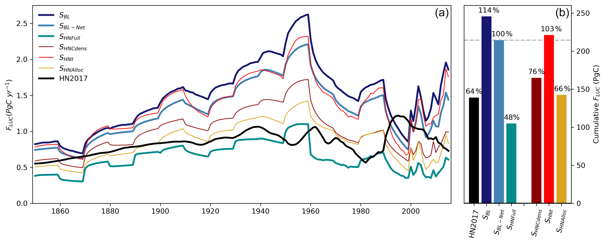
Figure 2Global FLUC between 1850 and 2015 (a) from the two bookkeeping model estimates in GCB2019 (HN2017 in black and SBL for BLUE in dark blue), the BLUE simulations with net LUC transitions and standard BLUE parameterisation (light blue, SBL-Net, used as reference for all subsequent BLUE runs) and using all tested HN2017 parameterisations together (cyan, SHNFull). The factorial simulations with only one set of parameters changed are shown in thin lines (SHNCdens in dark red, SHNt in red, SHNAlloc in yellow). The corresponding cumulative totals between 1850 and 2015 are shown in panel (b), and values relative to SBL-Net are shown by the numbers above bars.
All BLUE simulations show similar interannual variability patterns, consistent with the use of the LUH2v2.1 forcing, but these variations are dampened when the parameters for C densities, allocation fractions and time constants from HN are used. The BLUE simulation using the full set of HN2017 parameters (SHNFull) shows FLUC close to those of HN2017 until the 1980s and with a weak peak in emissions in 1960s and relatively stable FLUC rather than an increasing trend in 2000–2015. The resulting cumulative FLUC for SHNFull is 104 PgC, 52 % lower than SBL-NET, at the low end of previous estimates (Hansis et al., 2015; Houghton et al., 2012). This value is substantially outside the cumulative budget range of the GCB2019 (205±60 PgC 1850–2018) but still consistent with the uncertainty range of ±0.7 PgC yr−1 provided by GCB2019 after 1959.
The parameters that lead to larger differences in global FLUC are the C densities (SHNCdens, Fig. 2, dark red) and the allocation rules (SHNAlloc, yellow), while changing the decay times have small effect. Both SHNCdens and SHNAlloc result in lower FLUC over the 1850–2015 period, and weaker increasing trends between 2000 and 2015, which indicates that the trends in this period are not only due to forcing differences (Bastos et al., 2020) but in part from model parameterisation. The cumulative FLUC in 1850–2015 is 164 and 142 PgC for SHNCdens and SHNAlloc respectively, i.e. 24 % and 34 % lower than SBL-Net, and closer to the HN2017 estimate on global scale. The lower FLUC with HN2017 C densities can be explained by the HN2017 lower C densities in both vegetation and soil for most PFTs and the smaller difference between primary and secondary forest C stocks (Table A2) compared to BLUE. In particular, BLUE often features higher vegetation carbon in broadleaf forests and higher soil carbon in most other ecosystems than HN2017, which, together with lower soil carbon assumed for cropland and pasture, leads to substantially larger carbon losses in BLUE for many transitions (Table A2). Even though SHNt results in a small positive difference in cumulative FLUC relative to SBL-NET (221 PgC), effect of response-curve times is multiplicative (Fig. 1), therefore the FLUC trends are amplified (Fig. 2, left panel).
3.2 Regional patterns
The global differences between simulations result from interactions between the different factors and in the types of LUC occurring in a given point in space and time. We first analyse the temporal evolution of regional FLUC for each simulation (Fig. 3).
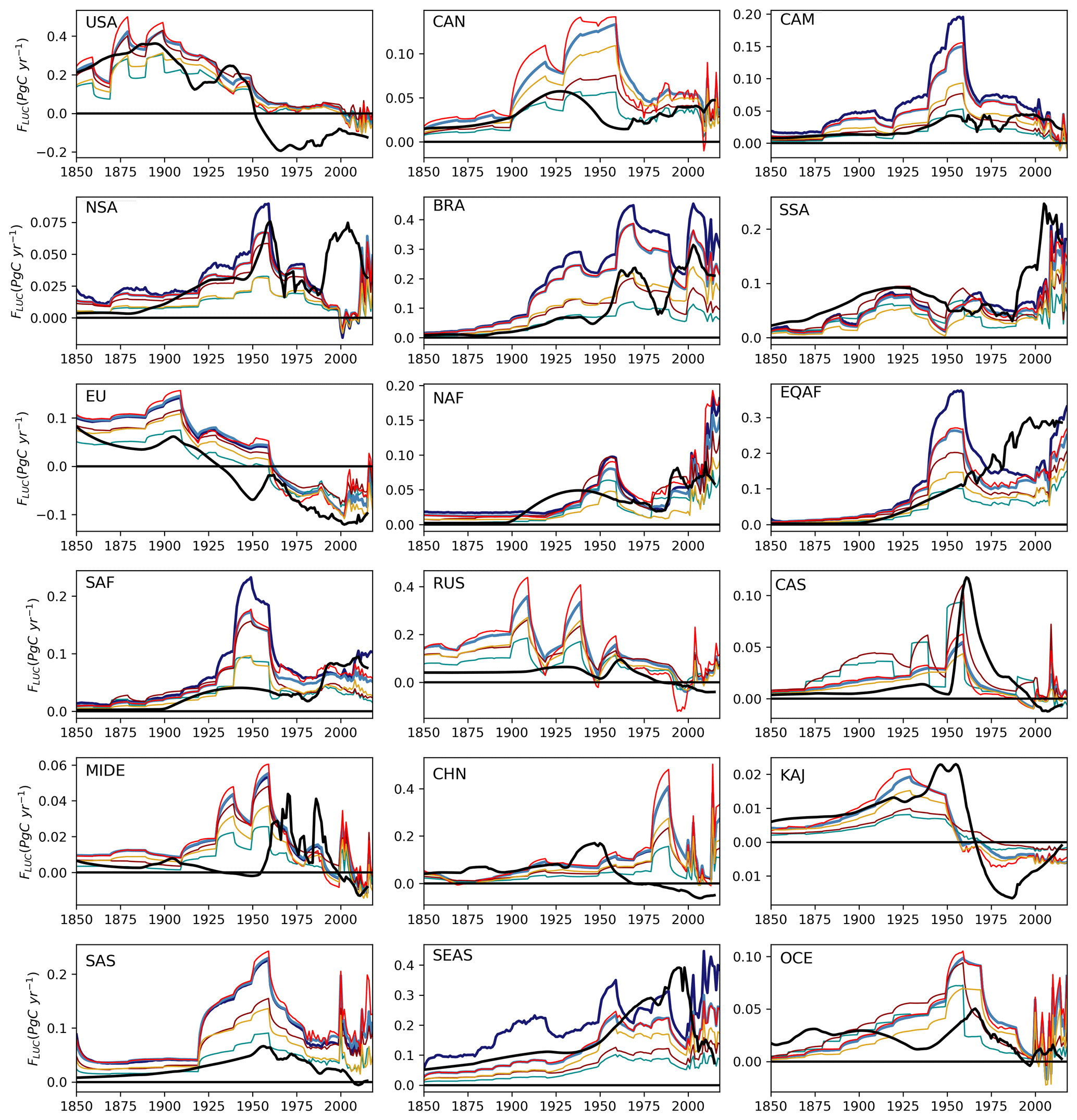
Figure 3Regional FLUC between 1850 and 2015 from the two BK model estimates in GCB2019 (HN2017 in black and SBL for BLUE in dark blue), the BLUE simulations with net LUC transitions and standard parameterisation (light blue, SBL-Net) and using HN2017 parameterisations (cyan, SHNFull). The factorial simulations with only one set of parameters changed are shown in thin lines (SHNCdens in dark red, SHNt in red, SHNAlloc in yellow).
The factorial analysis sheds light on the underlying reasons of the diverging trends in the 2000s, where BLUE showed an upward trend, opposing the downward trend in FLUC from HN2017. In absolute terms, the upward trend in BLUE stems foremost from BRA (a peak of about 0.45 PgC yr−1 in the early 2000s, then a decline; similar in HN2017 but peaking at about 0.3 PgC yr−1), SSA (also captured by HN2017 but accelerating from the 2000s to the 2010s in BLUE, decelerating in HN2017), NAF (by comparison more stable in HN2017), EQAF (similar values as in HN2017 but with 0.15 PgC yr−1 FLUC in BLUE in the 1970s–2000s is only about half that of HN2017) and SEAS (where HN2017 has a peak in the 1990s, then a steep drop of 0.3 PgC yr−1 to 2015, while BLUE FLUC picks up by about 0.2 PgC yr−1 over the 2000s). Additionally, BLUE shows an increase in FLUC in CHN for the 2010s, while HN2017 estimates a sink due to afforestation. In all of these regions, adjusting BLUE partly or fully to HN2017 parameters does not obviously bring trends closer together, because a lowering of the 2000s FLUC in BLUE, which results from several of the factorial experiments, would lead to lower FLUC in earlier time periods as well.
To summarise these patterns, we calculate the relative average differences in regional cumulative FLUC from SBL-Net and SHNFull with SBL (top panel of Fig. 4a, values in percent change) and the root mean square difference with HN2017 (Eq. 1, RMSDHN-BLUE), which reflects differences in interannual variability (top panel of Fig. 4b, in TgC yr−1).
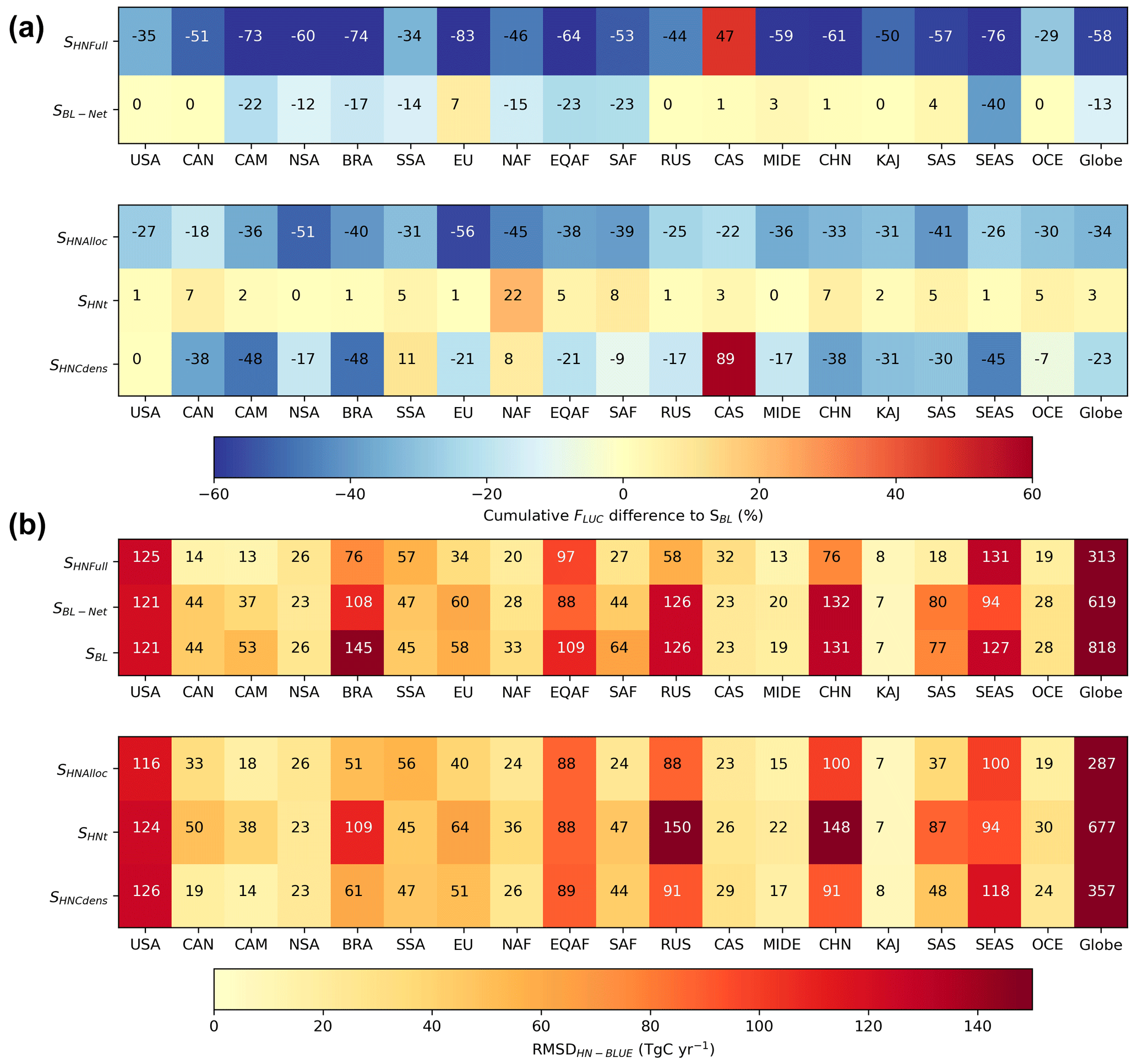
Figure 4(a) Relative changes in cumulative simulated FLUC between 1850–2015 for each region for SBL-Net and SHNFull compared to SBL (top two rows) and the relative effect of each parameter change, compared to SBL-NET (bottom three rows) indicated by the colours and numbers in the centre of cells. (b) The RMSDHN-BLUE for each simulation indicated by the colours and numbers in the centre of cells. All panels show results for the period 1850–2015.
Even though SBL-Net results in a small (−13 %) decrease in global FLUC compared to SBL as discussed above, regional differences show stronger decreases, especially in regions with intensive shifting cultivation practices, such as SEAS (−40 %), CAM (−22 %), SAF and EQAF (−23 % in both). SBL-Net additionally leads to higher agreement in interannual variability with HN2017 at global scale but also for most regions (i.e. lower RMSDHN-BLUE, Fig. 4b). Europe shows 7 % higher cumulative FLUC for SBL-Net than SBL, likely because of the importance of subpixel post-abandonment recovery and re-/afforestation dynamics in Europe (Bayer et al., 2017; Fuchs et al., 2015). However, this increases the RMSDHN-BLUE by only 2 TgC yr−1.
As seen for global FLUC, the simulation using HN2017 parameter values (SHNFull) leads to a reduction of FLUC by 50 % or more compared to SBL in many regions (dark blue colours, see values in the centre of grid cells in Fig. 4a), except for CAS, where an increase of 47 % is estimated, mainly due to differences in C density parameters. The reductions in cumulative FLUC differences in CAM, BRA, EU and SEAS. Decreases in the RMSDHN-BLUE between SHNFull and SBL-Net globally and for 11 of the 18 regions (Fig. 4b), with small increases elsewhere. This shows that differences in setup and parameterisation cancel differences arising from the different land-use forcing in BLUE and HN2017 in some regions. In addition, the reductions in RMSDHN-BLUE in SHNFull compared to SBL are stronger than for SBL-Net, indicating that parameterisation differences have stronger contribution to RMSDHN-BLUE than the impact of simulation net/gross transitions.
The differences between SBL-Net and each of the factorial simulations (bottom panel of Fig. 4a) shows that C densities and allocation rules are the dominant factors not just for global FLUC, but also in most regions, and lead to lower RMSDHN-BLUE, compared to SBL-Net (Fig. 4b). Using HN2017 allocation fractions to pools for harvest and clearing results in lower cumulative FLUC everywhere (SHNAlloc) and decreases the RMSDHN-BLUE at global scale and in all regions but NSA and SSA. Altering C densities (SHNCdens) has contrasting effects in cumulative FLUC between regions, increasing cumulative FLUC in 3 out of 18 regions. Strong reductions in RMSDHN-BLUE for SHNFull are found in BRA, RUS, CHN and SAS (top panel in Fig. 4b), explained by RMSDHN-BLUE reductions by changing the C densities in vegetation and soil pools (SHNCdens) and allocation fractions. In SEAS, cumulative FLUC is reduced when using HN2017 parameters (SHNFull) but with a higher RMSDHN-BLUE. In this region, C density parameters contribute the most to the reduction of bias, compared to SBL-Net, and both C density parameters and allocation fractions contribute to the increase in RMSDHN-BLUE. This highlights the importance of interactions between different parameters to the overall FLUC variability. The decay times generally contribute to small increases in cumulative FLUC compared to SBL-Net, except NAF where they increase FLUC by 22 % and would slightly amplify RMSDHN-BLUE globally and in 13 of the 18 regions.
3.3 Effects on gross FLUC component fluxes
To better understand the effects of the different parameterisations on FLUC, we analyse the spatial distribution of the differences between SHNFull, SHNCdens, SHNAlloc, SHNt and SBL-Net decomposed into gross FLUC: fluxes from harvest, clearing, abandonment/regrowth and transitions between crop and pasture (Fig. 5).

Figure 5Spatial distribution of relative differences in average FLUC between 1850–2018 for each of the four simulations with HN2017 parameters (SHNFull, SHNCdens, SHNAlloc, SHNt), compared to SBL-Net for different FLUC components: wood harvest, abandonment, clearing and crop–pasture transitions. Regions with average low values of FLUC (e.g. deserts) are masked.
In most grid cells, the difference between SHNFull and SBL-Net is dominated by the effects of the parameterisation of C densities in gross fluxes and allocation rules for abandonment fluxes. For FLUC from abandonment and clearing to agriculture (crop and pasture), the differences are mostly negative (i.e. higher uptake from recovery and lower emissions from clearing to agriculture using HN2017 parameterisation), while for the fluxes from transitions between crop and pastures and harvest, regional contrasts between positive and negative differences are found. The lower FLUC from clearing to agriculture for SHNFull in most grid cells is linked with the lower vegetation and soil C densities for most forest PFTs (Table A2). Higher FLUC from wood harvest are simulated by SHNFull in eastern and northern North America, central Europe and Scandinavia and China, mostly related with response-curve time constants. Other transitions (crop to pasture or pasture to crop) result in higher FLUC for SHNFull in most semi-arid regions, which is explained to a larger extent by differences in C densities and time constants between the two models (SHNCdens, SHNt) than by allocation rules (SHNAlloc) (Table A2).
Fluxes from land-use change and management are one of the most uncertain and least constrained components of the global carbon cycle (Bastos et al., 2020; Friedlingstein et al., 2019; Houghton, 2020). Several sources of uncertainty in FLUC have been previously analysed, such as the choice of gross vs. net LUC transitions (Bayer et al., 2017; Fuchs et al., 2015; Gasser et al., 2020; Wilkenskjeld et al., 2014), the definitions and terminology used (Grassi et al., 2018; Pongratz et al., 2014) or the management processes considered (Arneth et al., 2017; Pugh et al., 2015). The two bookkeeping models used in the global carbon budgets may differ in their FLUC estimates due to differences in the forcing data and differences in model structure, parameterisation and in how certain processes are represented. The impact of the LUC forcing on FLUC has been extensively investigated in previous studies (Bastos et al., 2020; Gasser et al., 2020; Hartung et al., 2021). Both models have a similar structure (Table 2) and both models use parameters from different sources that are based on observations which are, however, uncertain. Here, we evaluate how the different model parameterisations impact FLUC estimates and whether they can explain differences in global and regional average FLUC and on variability between the two models since 1850.
The simulation with net transition (SBL-Net) reduces differences in the average and interannual variability of FLUC estimates from BLUE and HN2017. The contribution of gross to FLUC is smaller than previous estimates (15 %–38 %, Arneth et al., 2017; Fuchs et al., 2015; Hansis et al., 2015) and also lower than in earlier BLUE simulations that used the same rule. Cancelling of primary and secondary land clearing, with primary first, gave 24 % lower emissions in Hansis et al. (2015). The differences are likely explained by the substantial changes that came in with the change from LUH1 to LUH2 versions, in particular the change to Heinimann et al. (2017) shifting cultivation maps.
Based on observation-based constraints by atmospheric inversions Bastos et al. (2020) pointed out that FLUC estimated by DGVMs and BLUE in BRA, SEAS, EU and EQAF were probably too high. Our analysis shows that FLUC estimates for these regions, except EU would be lower if the setup of HN2017 were used, i.e. starting in 1700 instead of 850 and using net transitions, and all four regions would show even larger reductions in FLUC if the parameterisation of HN2017 were used in BLUE. However, these changes would also bring down FLUC estimates in many regions that were not deemed too high in FLUC based on the constraint by observations. This suggests that neither the BLUE nor HN2017 setup and parameterisation can be judged as being superior to the other for all regions of the world and all time periods.
The rules for allocation of displaced carbon to different pools have the strongest effect on average FLUC, as well as their variability, followed by C density parameters. Contrary to C densities (Sect. 4.1), at the moment no global dataset of allocation parameters exists that could be compared to the allocation fractions used here. BLUE and HN2017 FLUC in 1850–2015 show better agreement in temporal variability, mostly because fact that the C density and allocation parameterisations of HN2017 dampen the effect of differences in land-use change transitions.
This elimination of the 2000s trend difference in some regions comes at the cost of larger divergences in earlier times. With high LUC dynamics in the 20th century in some regions, which is more strongly captured by BLUE with its representation of gross transitions, slightly larger C density losses with the transformation of natural vegetation to agriculture or degradation by wood harvesting and rangelands may lead to an increase in FLUC beyond what would be expected from net land-use areas alone. On top comes a distribution of cleared and harvested material to faster pools (more slash in BLUE, more long-lived products in HN2017), which also emphasises the effects of LUC dynamics. The differences between BLUE and HN2017 are thus a combination of higher LUC dynamics in BLUE (by using LUH2v2.1 and accounting for gross transitions) and of faster material decay than in HN2017. The different trends of BLUE and HN2017 in the 1950s and after 1990 are instead largely attributable to the different LUC forcing (Gasser et al., 2020).
4.1 Constraining C densities
The parameterisation of C densities of vegetation and soil pools is the second most relevant parameter but one that affects all flux components. Even though both models were parameterised based on observation-based C densities, these parameters are highly uncertain, as they are derived from sparse plot-level data with high variance across datasets (Brown and Lugo, 1982; Post et al., 1982; Schlesinger, 1984; Zinke et al., 1986). Remote-sensing-based estimates of potential vegetation C stocks in undisturbed lands and well as present-day C stocks have been produced by Erb et al. (2018), including their uncertainty. The values of Erb et al. (2018) can, therefore, be compared to the potential C stocks simulated by HN2017 and by BLUE using the different configurations in this study (circles in Fig. 6), as well as of simulated present-day carbon stocks (small circles, end of arrows). In addition, we compare simulated C stocks with those of Anav et al. (2013) for the present day.
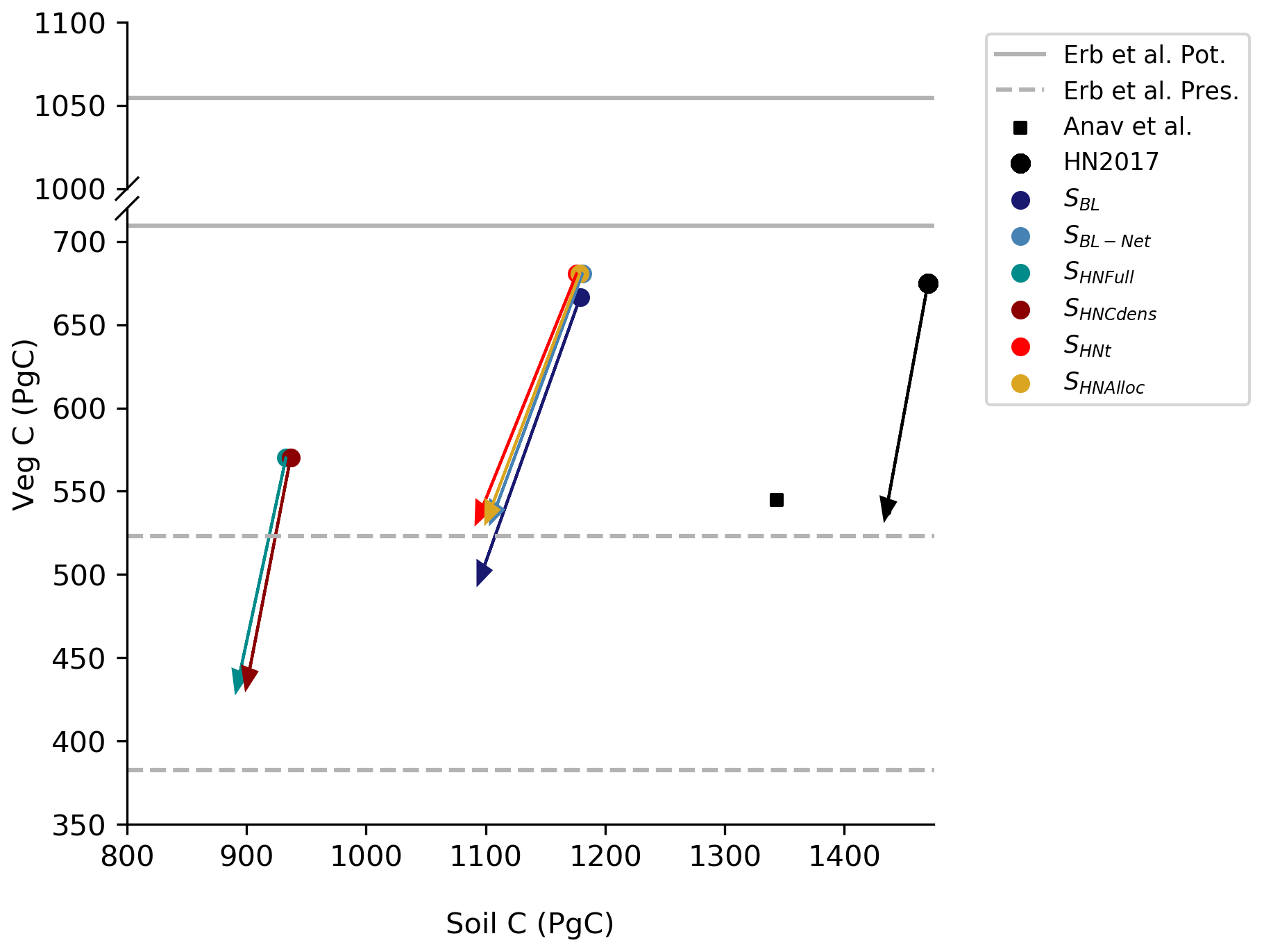
Figure 6Carbon stocks in vegetation (y axis) and soils (x axis) simulated by BLUE for the pre-industrial period (1850, big circles) and present time (2018, small circles, end of arrows). These values are compared to two observation-based reference datasets: that of Anav et al. (2013) for both vegetation and soil carbon stocks (black square) and the upper and lower values of potential (solid lines) and present-day (dashed lines) carbon stocks in vegetation from Erb et al. (2018).
All BLUE simulations, as well as HN2017, have 4 %–6 % lower potential C stocks in vegetation than estimates in Erb et al. (2018) (Fig. 6). Since the values of potential biomass in Erb et al. (2018) were estimated for present day, they include the effect of environmental changes such as CO2 fertilisation, and are expected to be up to 10 % higher than they would be without these effects (Pongratz et al., 2014). Therefore, the C stocks in vegetation simulated both by BLUE and HN2017 are consistent with these remote-sensing based estimates, if environmental effects are excluded. The methodology of using the highest percentiles in a moving window as a potential value in Erb et al. (2018) could overestimate biomass because it has a bias towards capturing the oldest rather than average forests in a cycle of natural disturbances. Additionally, these simulations result in present-day C stocks in vegetation that are within the range provided by Erb et al. (2018), or close to its upper limit, and are also consistent with the reference value from Anav et al. (2013). All simulations estimate lower C stocks in the soil, compared to Anav et al. (2013). HN2017 has higher C stocks in soil both for the pre-industrial period and the present day, compared to BLUE simulations, which are close to the values estimated by Anav et al. (2013). The two simulations using HN2017 carbon densities (SHNFull, and SHNCdens) result in too-low C stocks in soils, compared to Anav et al. (2013), and much lower potential vegetation C stocks than Erb et al. (2018). However, present-day vegetation C stocks for SHNFull and SHNCdens are consistent with their values.
We conclude that differences between BLUE and HN2017 arise from the higher allocation of cleared and harvested material to quickly decomposing pools in BLUE, compared to HN2017, combined with higher emissions in BLUE due to often larger differences in soil and vegetation C densities between natural and managed vegetation or primary and secondary vegetation. It should be noted, however, that specific transitions and prevalence of specific PFTs in certain regions prohibits generalising this statement. Together with the larger land-use dynamics which stem from BLUE representing gross transitions and its usage of LUH2v2.1 as LUC forcing, these changes lead to overall higher carbon losses that have a faster decay.
The two reference datasets of global C stocks seem to support the choice of C densities used in the default BLUE configuration and therefore the higher estimates of FLUC by BLUE. However, it should be noted that both models have limited representation of spatial variability in C densities: BLUE ignores spatial variability in vegetation and soil C within each PFT distribution, for example, due to less favourable climate in some regions; HN2017 includes country-specific C densities for vegetation, but not for soil, and no spatial variability within each country.
The large contribution of the C densities to the differences between the FLUC estimates of the two BK models found in our results highlights the importance of deriving spatially explicit maps of vegetation, and soil C densities discriminated per vegetation type would be required. Producing such maps is challenging, especially for the estimates of C densities in undisturbed land, as most of the land surface has been directly or indirectly impacted by human activity. However, observation-based maps of vegetation and soil C densities in both disturbed and undisturbed land would be highly valuable, as they could be used in BK models to reduce uncertainties in FLUC.
Similarly, improvements in allocation can be performed. Bookkeeping models, and many DGVMs, follow very simple assumptions of the fate of cleared or harvested material, often along the lines of the “Grand Slam Protocol” (McGuire et al., 2001) but developed for bookkeeping models earlier (Houghton et al., 1983), which distinguishes only three product pools (fast, medium, slow), with timescales defined rather ad hoc as 1, 10 or 100 years. The fractions going into these and into slash are compiled from individual studies for specific regions (Houghton et al., 1983; Hurtt et al., 2020) but are hard to quantify on the global level throughout several centuries. Such long timescales are needed, however, to capture the slow dynamics of decay and regrowth and thus to capture legacy fluxes accurately. For the last decades, however, more detailed data have become available than those currently used in the models of the global carbon budgets, such as global sets of dynamic carbon-storage factors (Mason Earles et al., 2012) that define a larger number of product pools and time-varying fractions of allocation.
Table A1Plant functional types in HN2017 and in BLUE, and the correspondence used in this study.
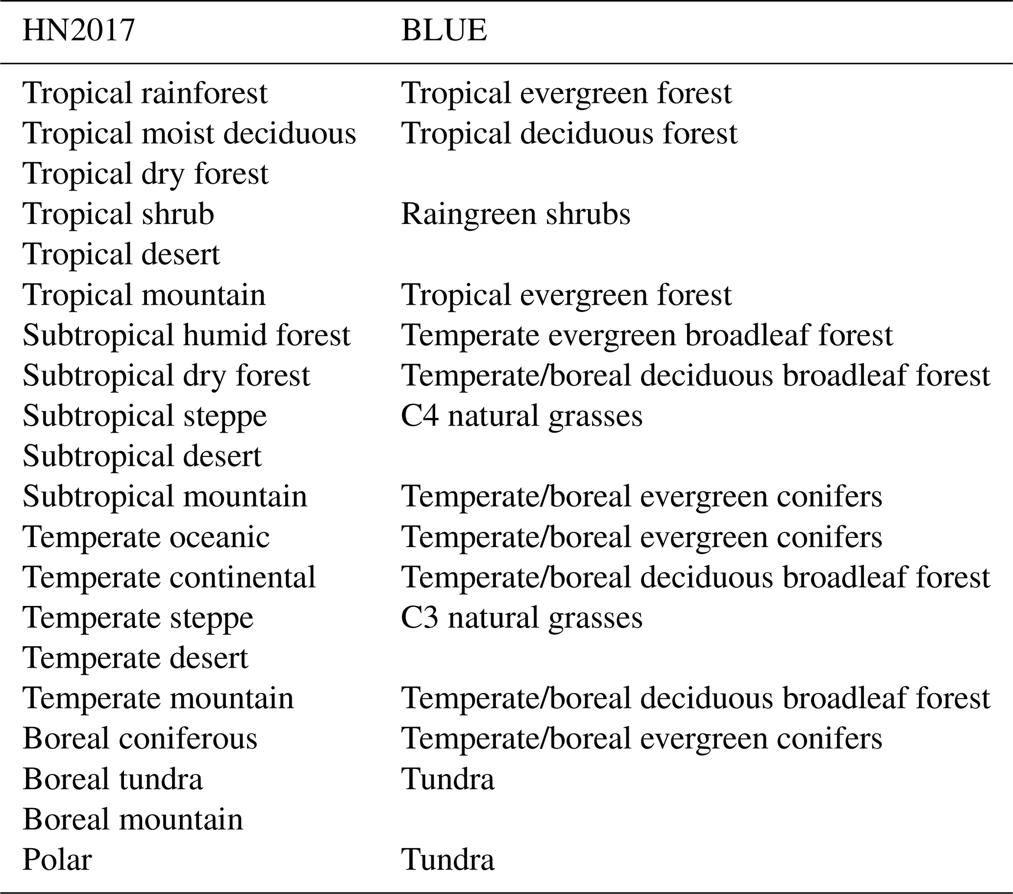
Table A2Global median value across countries per PFT for vegetation C densities and PFT-dependent soil C densities from BLUE, and from HN2017 converted to BLUE PFT classes as used for the simulations with parameters from HN2017. Units are tC ha−1.
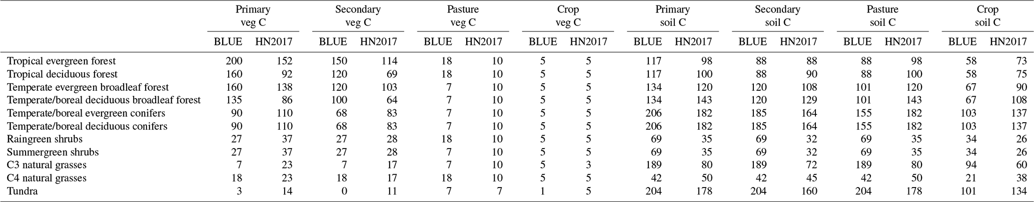
Table A3Global median values of harvest and clearing allocation rules to the short-, medium- and long-lived pools (1, 10 and 100 years) for BLUE PFTs, from the standard BLUE setup and used for the simulations with parameters from HN2017 (converted to BLUE PFT classes). The slash fraction from clearing is calculated as the 1 minus the sum of the 1-, 10- and 100-year pools.

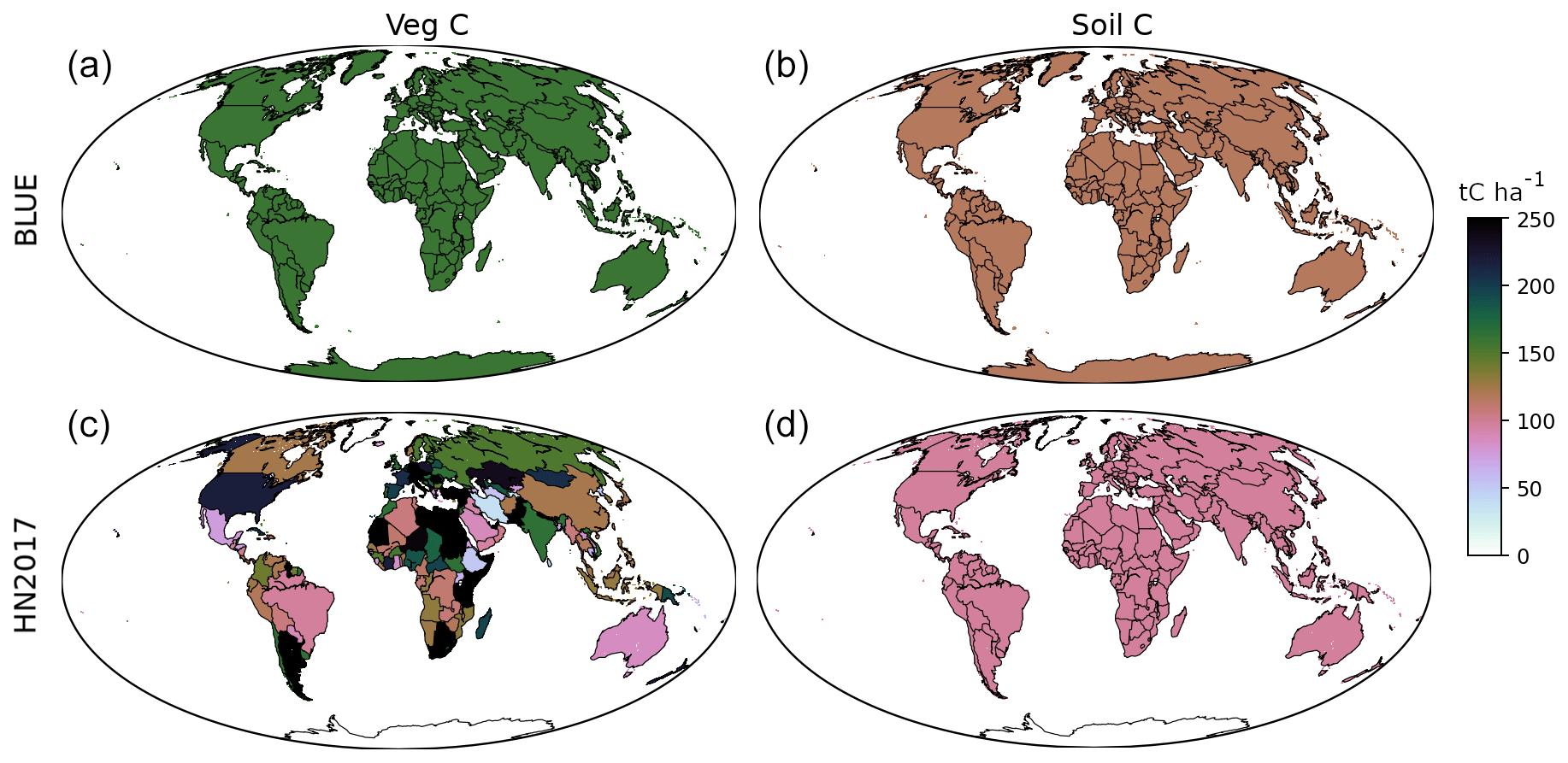
Figure A1Carbon densities in vegetation (a, c) and soil (b, d) for tropical broadleaved evergreen forests for BLUE (a, b) and HN2017 (c, d) in tC ha−1. It should be noted that even though C density values are assigned on a per-country basis in HN2017, they do not differ between countries for soil C. Note that C densities are assigned to all countries, even if evergreen broadleaved forest is not present in a given country.
The bookkeeping model code can be requested from Richard A. Houghton (HN2017) and Julia Pongratz (BLUE). Other scripts are available upon request to the corresponding author.
The global and regional fluxes from HN2017 and the BLUE simulations are provided in the Supplement. The gridded fields of the BLUE simulations can be provided by the contact author upon request.
The supplement related to this article is available online at: https://doi.org/10.5194/esd-12-745-2021-supplement.
AB designed the study together with JP, with input from KH, JEMSN and TBN. AB planned and executed the model simulations as well as the overall analysis. RAH and JP provided expert knowledge on each of the two bookkeeping models. TBN prepared Fig. 1. KH, JP, RAH and JEMSN contributed to the discussion of the results. AB prepared the original draft; all other co-authors participated in the review and editing of the paper.
The authors declare that they have no conflict of interest.
Publisher's note: Copernicus Publications remains neutral with regard to jurisdictional claims in published maps and institutional affiliations.
We thank Andrea Castanho and Alexander A. Nassikas for support in extracting parameters from the HN2017 model.
The article processing charges for this open-access publication were covered by the Max Planck Society.
This paper was edited by Zhenghui Xie and reviewed by two anonymous referees.
Anav, A., Friedlingstein, P., Kidston, M., Bopp, L., Ciais, P., Cox, P., Jones, C., Jung, M., Myneni, R., and Zhu, Z.: Evaluating the Land and Ocean Components of the Global Carbon Cycle in the CMIP5 Earth System Models, J. Climate, 26, 6801–6843, https://doi.org/10.1175/JCLI-D-12-00417.1, 2013.
Arneth, A., Sitch, S., Pongratz, J., Stocker, B., Ciais, P., Poulter, B., Bayer, A., Bondeau, A., Calle, L., Chini, L. P., Gasser, T., Fader, M., Friedlingstein, P., Kato, E., Li, W., Lindeskog, M., Nabel, J. E. M. S., Pugh, T. A. M., Robertson, E., Viovy, N., Yue, C., and Zaehle, S.: Historical carbon dioxide emissions caused by land-use changes are possibly larger than assumed, Nat. Geosci., 10, 79–84, https://doi.org/10.1038/ngeo2882, 2017.
Bastos, A., Ciais, P., Barichivich, J., Bopp, L., Brovkin, V., Gasser, T., Peng, S., Pongratz, J., Viovy, N., and Trudinger, C. M.: Re-evaluating the 1940s CO2 plateau, Biogeosciences, 13, 4877–4897, https://doi.org/10.5194/bg-13-4877-2016, 2016.
Bastos, A., O'Sullivan, M., Ciais, P., Makowski, D., Sitch, S., Friedlingstein, P., Chevallier, F., Rödenbeck, C., Pongratz, J., and Luijkx, I.: Sources of uncertainty in regional and global terrestrial CO2-exchange estimates, Global Biogeochem. Cy., 34, e2019GB006393, https://doi.org/10.1029/2019GB006393, 2020.
Bayer, A. D., Lindeskog, M., Pugh, T. A. M., Anthoni, P. M., Fuchs, R., and Arneth, A.: Uncertainties in the land-use flux resulting from land-use change reconstructions and gross land transitions, Earth Syst. Dynam., 8, 91–111, https://doi.org/10.5194/esd-8-91-2017, 2017.
Brown, S. and Lugo, A. E.: The Storage and Production of Organic Matter in Tropical Forests and Their Role in the Global Carbon Cycle, Biotropica, 14, 161–187, https://doi.org/10.2307/2388024, 1982.
Di Vittorio, A. V., Shi, X., Bond-Lamberty, B., Calvin, K., and Jones, A.: Initial Land Use/Cover Distribution Substantially Affects Global Carbon and Local Temperature Projections in the Integrated Earth System Model, Global Biogeochem. Cy., 34, e2019GB006383, https://doi.org/10.1029/2019GB006383, 2020.
Erb, K.-H., Kastner, T., Plutzar, C., Bais, A. L. S., Carvalhais, N., Fetzel, T., Gingrich, S., Haberl, H., Lauk, C., Niedertscheider, M., Pongratz, J., Thurner, M., and Luyssaert, S.: Unexpectedly large impact of forest management and grazing on global vegetation biomass, Nature, 553, 73–76, https://doi.org/10.1038/nature25138, 2018.
FAO: Global Forest Resources Assessment 2015 (FRA2015), Food and Agriculture Organization of the United Nations, Rome, 2015.
FAOSTAT: FAOSTAT: Food and Agriculture Organization of the United Nations, Rome, Italy, 2015.
Friedlingstein, P., Jones, M. W., O'Sullivan, M., Andrew, R. M., Hauck, J., Peters, G. P., Peters, W., Pongratz, J., Sitch, S., Le Quéré, C., Bakker, D. C. E., Canadell, J. G., Ciais, P., Jackson, R. B., Anthoni, P., Barbero, L., Bastos, A., Bastrikov, V., Becker, M., Bopp, L., Buitenhuis, E., Chandra, N., Chevallier, F., Chini, L. P., Currie, K. I., Feely, R. A., Gehlen, M., Gilfillan, D., Gkritzalis, T., Goll, D. S., Gruber, N., Gutekunst, S., Harris, I., Haverd, V., Houghton, R. A., Hurtt, G., Ilyina, T., Jain, A. K., Joetzjer, E., Kaplan, J. O., Kato, E., Klein Goldewijk, K., Korsbakken, J. I., Landschützer, P., Lauvset, S. K., Lefèvre, N., Lenton, A., Lienert, S., Lombardozzi, D., Marland, G., McGuire, P. C., Melton, J. R., Metzl, N., Munro, D. R., Nabel, J. E. M. S., Nakaoka, S.-I., Neill, C., Omar, A. M., Ono, T., Peregon, A., Pierrot, D., Poulter, B., Rehder, G., Resplandy, L., Robertson, E., Rödenbeck, C., Séférian, R., Schwinger, J., Smith, N., Tans, P. P., Tian, H., Tilbrook, B., Tubiello, F. N., van der Werf, G. R., Wiltshire, A. J., and Zaehle, S.: Global Carbon Budget 2019, Earth Syst. Sci. Data, 11, 1783–1838, https://doi.org/10.5194/essd-11-1783-2019, 2019.
Fuchs, R., Herold, M., Verburg, P. H., Clevers, J. G. P. W., and Eberle, J.: Gross changes in reconstructions of historic land cover/use for Europe between 1900 and 2010, Global Change Biol., 21, 299–313, https://doi.org/10.1111/gcb.12714, 2015.
Gasser, T. and Ciais, P.: A theoretical framework for the net land-to-atmosphere CO2 flux and its implications in the definition of “emissions from land-use change”, Earth Syst. Dynam., 4, 171–186, https://doi.org/10.5194/esd-4-171-2013, 2013.
Gasser, T., Crepin, L., Quilcaille, Y., Houghton, R. A., Ciais, P., and Obersteiner, M.: Historical CO2 emissions from land use and land cover change and their uncertainty, Biogeosciences, 17, 4075–4101, https://doi.org/10.5194/bg-17-4075-2020, 2020.
Grassi, G., House, J., Kurz, W. A., Cescatti, A., Houghton, R. A., Peters, G. P., Sanz, M. J., Viñas, R. A., Alkama, R., Arneth, A., Bondeau, A., Dentener, F., Fader, M., Federici, S., Friedlingstein, P., Jain, A. K., Kato, E., Koven, C. D., Lee, D., Nabel, J. E. M. S., Nassikas, A. A., Perugini, L., Rossi, S., Sitch, S., Viovy, N., Wiltshire, A., and Zaehle, S.: Reconciling global-model estimates and country reporting of anthropogenic forest CO2 sinks, Nat. Clim. Change, 8, 914–920, https://doi.org/10.1038/s41558-018-0283-x, 2018.
Hansis, E., Davis, S. J., and Pongratz, J.: Relevance of methodological choices for accounting of land use change carbon fluxes, Global Biogeochem. Cy., 29, 1230–1246, https://doi.org/10.1002/2014GB004997, 2015.
Hartung, K., Bastos, A., Chini, L., Ganzenmüller, R., Havermann, F., Hurtt, G. C., Loughran, T., Nabel, J. E. M. S., Nützel, T., Obermeier, W. A., and Pongratz, J.: Net land-use change carbon flux estimates and sensitivities – An assessment with a bookkeeping model based on CMIP6 forcing, Earth Syst. Dynam. Discuss. [preprint], https://doi.org/10.5194/esd-2020-94, in review, 2021.
Heinimann, A., Mertz, O., Frolking, S., Christensen, A. E., Hurni, K., Sedano, F., Chini, L. P., Sahajpal, R., Hansen, M., and Hurtt, G.: A global view of shifting cultivation: Recent, current, and future extent, PLOS One, 12, e0184479, https://doi.org/10.1371/journal.pone.0184479, 2017.
Hooijer, A., Page, S., Canadell, J. G., Silvius, M., Kwadijk, J., Wösten, H., and Jauhiainen, J.: Current and future CO2 emissions from drained peatlands in Southeast Asia, Biogeosciences, 7, 1505–1514, https://doi.org/10.5194/bg-7-1505-2010, 2010.
Houghton, R. and Nassikas, A. A.: Global and regional fluxes of carbon from land use and land cover change 1850–2015, Global Biogeochem. Cy., 31, 456–472, https://doi.org/10.1002/2016GB005546, 2017.
Houghton, R., Hobbie, J., Melillo, J. M., Moore, B., Peterson, B., Shaver, G., and Woodwell, G.: Changes in the Carbon Content of Terrestrial Biota and Soils between 1860 and 1980: A Net Release of CO2 to the Atmosphere, Ecol. Monogr., 53, 235–262, https://doi.org/10.2307/1942531, 1983.
Houghton, R. A.: Terrestrial Fluxes of Carbon in GCP Carbon Budgets, Global Change Biol., 26, 3006–3014, https://doi.org/10.1111/gcb.15050, 2020.
Houghton, R. A., House, J. I., Pongratz, J., van der Werf, G. R., DeFries, R. S., Hansen, M. C., Le Quéré, C., and Ramankutty, N.: Carbon emissions from land use and land-cover change, Biogeosciences, 9, 5125–5142, https://doi.org/10.5194/bg-9-5125-2012, 2012.
Hurtt, G. C., Chini, L., Sahajpal, R., Frolking, S., Bodirsky, B. L., Calvin, K., Doelman, J. C., Fisk, J., Fujimori, S., Klein Goldewijk, K., Hasegawa, T., Havlik, P., Heinimann, A., Humpenöder, F., Jungclaus, J., Kaplan, J. O., Kennedy, J., Krisztin, T., Lawrence, D., Lawrence, P., Ma, L., Mertz, O., Pongratz, J., Popp, A., Poulter, B., Riahi, K., Shevliakova, E., Stehfest, E., Thornton, P., Tubiello, F. N., van Vuuren, D. P., and Zhang, X.: Harmonization of global land use change and management for the period 850–2100 (LUH2) for CMIP6, Geosci. Model Dev., 13, 5425–5464, https://doi.org/10.5194/gmd-13-5425-2020, 2020.
IPCC: Climate Change and Land: an IPCC special report on climate change, desertification, land degradation, sustainable land management, food security, and greenhouse gas fluxes in terrestrial ecosystems, edited by: Shukla, P. R., Skea, J., Calvo Buendia, E., Masson-Delmotte,V., Pörtner, H.-O., Roberts, D. C., Zhai, P., Slade, R., Connors, S., van Diemen, R., Ferrat, M., Haughey, E., Luz, S., Neogi, S., Pathak, M., Petzold, J., Portugal Pereira, J., Vyas, P., Huntley, E., Kissick, K., Belkacemi, M., and Malley, J., available at: https://www.ipcc.ch/site/assets/uploads/2019/11/SRCCL-Full-Report-Compiled-191128.pdf (last access: 28 June 2021), 2019.
Klein Goldewijk, K., Beusen, A., Doelman, J., and Stehfest, E.: Anthropogenic land use estimates for the Holocene – HYDE 3.2, Earth Syst. Sci. Data, 9, 927–953, https://doi.org/10.5194/essd-9-927-2017, 2017.
Le Quéré, C., Andrew, R. M., Friedlingstein, P., Sitch, S., Pongratz, J., Manning, A. C., Korsbakken, J. I., Peters, G. P., Canadell, J. G., Jackson, R. B., Boden, T. A., Tans, P. P., Andrews, O. D., Arora, V. K., Bakker, D. C. E., Barbero, L., Becker, M., Betts, R. A., Bopp, L., Chevallier, F., Chini, L. P., Ciais, P., Cosca, C. E., Cross, J., Currie, K., Gasser, T., Harris, I., Hauck, J., Haverd, V., Houghton, R. A., Hunt, C. W., Hurtt, G., Ilyina, T., Jain, A. K., Kato, E., Kautz, M., Keeling, R. F., Klein Goldewijk, K., Körtzinger, A., Landschützer, P., Lefèvre, N., Lenton, A., Lienert, S., Lima, I., Lombardozzi, D., Metzl, N., Millero, F., Monteiro, P. M. S., Munro, D. R., Nabel, J. E. M. S., Nakaoka, S., Nojiri, Y., Padin, X. A., Peregon, A., Pfeil, B., Pierrot, D., Poulter, B., Rehder, G., Reimer, J., Rödenbeck, C., Schwinger, J., Séférian, R., Skjelvan, I., Stocker, B. D., Tian, H., Tilbrook, B., Tubiello, F. N., van der Laan-Luijkx, I. T., van der Werf, G. R., van Heuven, S., Viovy, N., Vuichard, N., Walker, A. P., Watson, A. J., Wiltshire, A. J., Zaehle, S., and Zhu, D.: Global Carbon Budget 2017, Earth Syst. Sci. Data, 10, 405–448, https://doi.org/10.5194/essd-10-405-2018, 2018a.
Le Quéré, C., Andrew, R. M., Friedlingstein, P., Sitch, S., Hauck, J., Pongratz, J., Pickers, P. A., Korsbakken, J. I., Peters, G. P., Canadell, J. G., Arneth, A., Arora, V. K., Barbero, L., Bastos, A., Bopp, L., Chevallier, F., Chini, L. P., Ciais, P., Doney, S. C., Gkritzalis, T., Goll, D. S., Harris, I., Haverd, V., Hoffman, F. M., Hoppema, M., Houghton, R. A., Hurtt, G., Ilyina, T., Jain, A. K., Johannessen, T., Jones, C. D., Kato, E., Keeling, R. F., Goldewijk, K. K., Landschützer, P., Lefèvre, N., Lienert, S., Liu, Z., Lombardozzi, D., Metzl, N., Munro, D. R., Nabel, J. E. M. S., Nakaoka, S., Neill, C., Olsen, A., Ono, T., Patra, P., Peregon, A., Peters, W., Peylin, P., Pfeil, B., Pierrot, D., Poulter, B., Rehder, G., Resplandy, L., Robertson, E., Rocher, M., Rödenbeck, C., Schuster, U., Schwinger, J., Séférian, R., Skjelvan, I., Steinhoff, T., Sutton, A., Tans, P. P., Tian, H., Tilbrook, B., Tubiello, F. N., van der Laan-Luijkx, I. T., van der Werf, G. R., Viovy, N., Walker, A. P., Wiltshire, A. J., Wright, R., Zaehle, S., and Zheng, B.: Global Carbon Budget 2018, Earth Syst. Sci. Data, 10, 2141–2194, https://doi.org/10.5194/essd-10-2141-2018, 2018b.
Li, W., MacBean, N., Ciais, P., Defourny, P., Lamarche, C., Bontemps, S., Houghton, R. A., and Peng, S.: Gross and net land cover changes based on plant functional types derived from the annual ESA CCI land cover maps, Earth Syst. Sci. Data, 10, 219–234, https://doi.org/10.5194/essd-10-219-2018, 2018.
Mason Earles, J., Yeh, S., and Skog, K.: Timing of carbon emissions from global forest clearance, Nat. Clim. Change, 2, 682–685, https://doi.org/10.1038/nclimate1535, 2012.
McGuire, A. D., Sitch, S., Clein, J. S., Dargaville, R., Esser, G., Foley, J., Heimann, M., Joos, F., Kaplan, J., Kicklighter, D. W., Meier, R. A., Melillo, J. M., Moore, B., Prentice, I. C., Ramankutty, N., Reichenau, T., Schloss, A., Tian, H., Williams, L. J., and Wittenberg, U.: Carbon balance of the terrestrial biosphere in the Twentieth Century: Analyses of CO2, climate and land use effects with four process-based ecosystem models, Global Biogeochem. Cy., 15, 183–206, https://doi.org/10.1029/2000GB001298, 2001.
Pongratz, J., Reick, C., Raddatz, T., and Claussen, M.: Effects of anthropogenic land cover change on the carbon cycle of the last millennium, Global Biogeochem. Cy., 23, GB4001, https://doi.org/10.1029/2009GB003488, 2009.
Pongratz, J., Reick, C. H., Houghton, R., and House, J.: Terminology as a key uncertainty in net land use and land cover change carbon flux estimates, Earth Syst. Dynam., 5, 177–195, https://doi.org/10.5194/esd-5-177-2014, 2014.
Post, W. M., Emanuel, W. R., Zinke, P. J., and Stangenberger, A. G.: Soil carbon pools and world life zones, Nature, 298, 156–159, https://doi.org/10.1038/298156a0, 1982.
Pugh, T., Arneth, A., Olin, S., Ahlström, A., Bayer, A., Goldewijk, K. K., Lindeskog, M., and Schurgers, G.: Simulated carbon emissions from land-use change are substantially enhanced by accounting for agricultural management, Environ. Res. Lett., 10, 124008, https://doi.org/10.1088/1748-9326/10/12/124008, 2015.
Ramankutty, N. and Foley, J. A.: Estimating historical changes in global land cover: Croplands from 1700 to 1992, Global Biogeochem. Cy., 13, 997–1027, https://doi.org/10.1029/1999GB900046, 1999.
Schlesinger, W. H.: Soil Organic Matter: a Source of Atmospheric CO2, in: The Role of Terrestrial Vegetation in the Global Carbon Cycle: Measurement by Remote Sensing, edited by: Woodwell, G. M., John Wiley & Sons Ltd, available at: https://scope.dge.carnegiescience.edu/SCOPE_23/SCOPE_23_3.2_chapter4_111-127.pdf (last access: 28 June 2021), 1984.
Stocker, B. and Joos, F.: Quantifying differences in land use emission estimates implied by definition discrepancies, Earth Syst. Dynam., 6, 731–744, https://doi.org/10.5194/esd-6-731-2015, 2015.
Stocker, B. D., Strassmann, K., and Joos, F.: Sensitivity of Holocene atmospheric CO2 and the modern carbon budget to early human land use: analyses with a process-based model, Biogeosciences, 8, 69–88, https://doi.org/10.5194/bg-8-69-2011, 2011.
van der Werf, G. R., Randerson, J. T., Giglio, L., van Leeuwen, T. T., Chen, Y., Rogers, B. M., Mu, M., van Marle, M. J. E., Morton, D. C., Collatz, G. J., Yokelson, R. J., and Kasibhatla, P. S.: Global fire emissions estimates during 1997–2016, Earth Syst. Sci. Data, 9, 697–720, https://doi.org/10.5194/essd-9-697-2017, 2017.
Wilkenskjeld, S., Kloster, S., Pongratz, J., Raddatz, T., and Reick, C. H.: Comparing the influence of net and gross anthropogenic land-use and land-cover changes on the carbon cycle in the MPI-ESM, Biogeosciences, 11, 4817–4828, https://doi.org/10.5194/bg-11-4817-2014,, 2014.
Zinke, P. J., Millemann, R. E., and Boden, T. A.: Worldwide organic soil carbon and nitrogen data, Carbon Dioxide Information Center, Environmental Sciences Division, Oak Ridge, USA, https://doi.org/10.2172/543663, 1986.
The requested paper has a corresponding corrigendum published. Please read the corrigendum first before downloading the article.
- Article
(4009 KB) - Full-text XML
- Corrigendum
- Companion paper
-
Supplement
(168 KB) - BibTeX
- EndNote