Modelled land use and land cover change emissions – a spatio-temporal comparison of different approaches

Quantifying the net carbon flux from land use and land cover changes (f_LULCC) is critical for understanding the global carbon cycle and, hence, to support climate change mitigation. However, large-scale f_LULCC is not directly measurable and has to be inferred from models instead, such as semi-empirical bookkeeping models and process-based dynamic global vegetation models (DGVMs). By definition, f_LULCC estimates are not directly comparable between these two different model types. As an important example, DGVM-based f_LULCC in the annual global carbon budgets is estimated under transient environmental forcing and includes the so-called loss of additional sink capacity (LASC). The LASC results from the impact of environmental changes on land carbon storage potential of managed land compared to potential vegetation and accumulates over time, which is not captured in bookkeeping models. The f_LULCC from transient DGVM simulations, thus, strongly depends on the timing of land use and land cover changes mainly because LASC accumulation is cut off at the end of the simulated period. To estimate the LASC, the f_LULCC from pre-industrial DGVM simulations, which is independent of changing environmental conditions, can be used. Additionally, DGVMs using constant present-day environmental forcing enable an approximation of bookkeeping estimates. Here, we analyse these three DGVM-derived f_LULCC estimations (under transient, pre-industrial, and present-day forcing) for 12 models within 18 regions and quantify their differences as well as climate- and CO₂-induced components and compare them to bookkeeping estimates. Averaged across the models, we find a global f_LULCC (under transient conditions) of 2.0±0.6 PgC yr⁻¹ for 2009–2018, of which ∼40 % are attributable to the LASC (0.8±0.3 PgC yr⁻¹). From 1850 onward, the f_LULCC accumulated to 189±56 PgC with 40±15 PgC from the LASC. Around 1960, the accumulating nature of the LASC causes global transient f_LULCC estimates to exceed estimates under present-day conditions, despite generally increased carbon stocks in the latter. Regional hotspots of high cumulative and annual LASC values are found in the USA, China, Brazil, equatorial Africa, and Southeast Asia, mainly due to deforestation for cropland. Distinct negative LASC estimates in Europe (early reforestation) and from 2000 onward in the Ukraine (recultivation of post-Soviet abandoned agricultural land), indicate that f_LULCC estimates in these regions are lower in transient DGVM compared to bookkeeping approaches. Our study unravels the strong dependence of f_LULCC estimates on the time a certain land use and land cover change event happened to occur and on the chosen time period for the forcing of environmental conditions in the underlying simulations. We argue for an approach that provides an accounting of the f_LULCC that is more robust against these choices, for example by estimating a mean DGVM ensemble f_LULCC and LASC for a defined reference period and homogeneous environmental changes (CO₂ only).

1 Introduction

Terrestrial ecosystems play an important role for the global carbon cycle as they act as substantial sinks and sources of carbon (C) (Keenan and Williams, 2018). In both directions, fluxes in the land carbon cycle have significantly been altered in previous centuries due to anthropogenic land use and land cover changes (LULCCs), in particular through deforestation driven by early agricultural expansion in the mid-latitudes, recent tropical deforestation, and recent forest expansion in the mid- and high latitudes (Klein Goldewijk et al., 2011). Since 1850, the accumulated global net flux from LULCC (f_LULCC) contributed approximately one-third of global anthropogenic CO₂ emissions and was the dominant source until the 1950s, when fossil fuel emissions drastically increased (Friedlingstein et al., 2019). Despite its decreasing relative contribution, f_LULCC comprises an important share of the global carbon budget (GCB) and might again account for the bulk of anthropogenic C emissions in the future, if fossil emissions can be drastically reduced as described in some socio-economic pathways (Popp et al., 2017; Krause et al., 2018). The f_LULCC may also gain an important role in the quest for negative CO₂ emissions technologies, with LULCCs such as reforestation and afforestation (denoted reforestation in the following) bearing significant potential to sequester atmospheric CO₂ (Griscom et al., 2017; Fuss et al., 2018; Sonntag et al., 2016; Arneth et al., 2017). Accordingly, f_LULCC quantification is essential to better understand global carbon cycle dynamics, to estimate future climate change, and to support the assessment of greenhouse gas reduction efforts (Friedlingstein et al., 2019).

There is so far no general agreement on a single valid definition and approach to assess the f_LULCC. This is because the f_LULCC cannot be directly measured on a global scale due to the co-occurrence with natural C sinks and sources. For example, in managed forests, C fluxes result from logging and subsequent regrowth, which is part of the f_LULCC, but also change in response to interannual variability or long-term trends in environmental conditions (Friedlingstein et al., 2019). Inventories or satellite-based measurements cannot distinguish C fluxes induced by LULCC from those induced by environmental changes. To separate these terms, models are applied. Here, various approaches exist. In the 2019 GCB of the Global Carbon Project (hereafter GCB2019; Friedlingstein et al., 2019), two bookkeeping models are used: “Bookkeeping of Land Use Emissions” (hereafter BLUE; Hansis et al., 2015) and “Houghton and Nassikas 2017” (hereafter H&N2017; Houghton and Nassikas, 2017). The bookkeeping mean f_LULCC in the GCB2019 is combined with the uncertainty derived from process-based dynamic global vegetation models (DGVMs). DGVMs exist in much larger numbers and their process-based methods to calculate C fluxes allow one to account for the interplay of multiple drivers on C fluxes, which bookkeeping models cannot do.

However, estimates from bookkeeping models and DGVMs are not directly comparable due to underlying assumptions on C stocks (Pongratz et al., 2014). Bookkeeping models are semi-empirical models that combine observation-based C densities with information on areas affected by different types of LULCCs and response curves characterizing the speed of C uptake and release after specific LULCCs to calculate the f_LULCC. In contrast, to isolate the LULCC effects from those of environmental changes, DGVM-based f_LULCC is generally estimated as the difference of net land C uptake from net biome productivity (NBP) between simulations with and without LULCC. Within the GCB2019, these simulations are conducted under transient environmental conditions (such as climate, CO₂ concentrations, and nitrogen deposition); therefore, synergistic fluxes between LULCCs and environmental changes are included.

The transient DGVM approach includes the loss of additional sink capacity (LASC), representing C fluxes in response to environmental changes on managed land (typically croplands with low C sink capacity and fast turnover rates) as compared to potential natural vegetation (typically forests with large C sink capacity and slower turnover rates; Gitz and Ciais, 2003; Pongratz et al., 2014; Gasser and Ciais, 2013; Peng et al., 2014). As an example, when an area that acted as C sink is deforested, the stored C is lost at harvest time corresponding to an instantaneous f_LULCC. The resulting agricultural area typically does not constitute a major sink. In the simulation without LULCCs, the forest persists and may increase its C density over time, storing additional C in its slow-turnover woody and soil C pools in response to favourable environmental changes such as increased CO₂ concentrations. Compared to the simulation without LULCC, the sink capacity would consequently be diminished in the simulation with LULCC. Thus, even though the instantaneous emissions of the deforestation event may have ceased, deforestation continues to alter the f_LULCC since the reference simulation assumes the potential vegetation cover in the absence of LULCCs and simulates its response to environmental changes. This example illustrates an interesting aspect of the LASC: it has been acknowledged that the LASC in its literal sense (a loss of carbon, positive LASC values) is an unrealized C uptake potential and is not reflected in any real change in atmospheric CO₂ concentration (Pongratz et al., 2014). However, as the LASC captures the foregone C sinks that were destroyed by a LULCC event (and likely accumulates even in absence of further LULCCs), it manifests in the budget of atmospheric CO₂ as compared to a reference excluding LULCCs (Pongratz et al., 2014). In contrast to the theoretical nature of positive LASC values, negative values counted towards the LASC, for example due to reforestation, depict realized C uptake that is theoretically observable (though observations in the field are highly complex due to co-occurrence of natural carbon fluxes).

The result of a permanent reduction of a C sink on the LASC, as due to deforestation, is difficult to predict over time. Natural C sinks are subject to changes and can even turn into C sources for periods of time, due to the interplay of multiple factors that control the C balance of ecosystems simultaneously. For example, the LASC may increase because of an increased C uptake via higher NBP resulting from atmospheric CO₂ increases (Albani et al., 2006; Schimel et al., 2015; or review of CO₂ effect in Walker et al., 2021) or global-warming-induced longer growing seasons in northern latitudes and higher altitudes (Keenan et al., 2014; O'Sullivan et al., 2020). Conversely, environmental driven decreases in C stock turnover times, for example due to an increased frequency and severity of drought and heat stress events (Bastos et al., 2020) or increased fire (included in some DGVMs of the GCB2019), may reduce NBP and thus may cause LASC decreases (and lower f_LULCC estimates). The LASC will thus differ in magnitude and direction over time and across space.

Environmentally induced C stock changes not only alter the LASC, but also the instantaneous f_LULCC. For example, the f_LULCC from clearing pristine forest is expected to be higher today than during pre-industrial times if the forest has grown denser over time. Additionally, legacy effects result from the ongoing adaption of ecosystems to historical environmental changes (Krause et al., 2020). Such transient environmental effects are excluded in bookkeeping approaches – either through using constant C densities, or through purposefully excluding alterations in C densities from transient DGVM simulations in reduced-complexity Earth system models (Gasser et al., 2020). The independence or dependence of vegetation and soil C densities from environmental conditions is thus another difference between transient DGVM and bookkeeping approaches. Here, DGVM simulations under constant environmental forcing can help to attribute f_LULCC quantities independent of the timing of LULCCs.

DGVM simulations under constant environmental conditions have been performed within the project “Trends and drivers of the regional-scale sources and sinks of carbon dioxide” (TRENDY; Le Quéré et al., 2013; Sitch et al., 2015), when conducting the simulations for the GCB2019 (Friedlingstein et al., 2019). This included a first set of simulations that quantify the f_LULCC based on constant present-day environmental conditions. This approach is more similar to bookkeeping estimates and can be evaluated against Earth observation or inventory data as it most closely represents the observable state under today's conditions and excludes transient flux alterations. Moreover, recent observations are commonly used to estimate the past, for example by combining observed C densities with vegetation coverage reconstructions to infer C stocks in human absence or with historical area changes for time series of C stock losses (Sanderman et al., 2017; Erb et al., 2018).

However, as f_LULCC quantities derived under constant present-day conditions are independent of long-term environmental trends, the increased C stocks due to spinup with present-day environmental conditions may lead to comparably higher f_LULCC estimates, especially in early simulation years (environmental changes during the industrial period, in general and on global scale, increased C stocks; refer to Fig. 1 for illustration). More realistic f_LULCC estimates for the early period can be derived assuming that pre-industrial environmental conditions prevailed over time (Pongratz et al., 2014; Stocker and Joos, 2015); however, despite being based on the same land use dataset, this leads to comparably lower f_LULCC estimates, in particular for later LULCCs (Stocker and Joos, 2015).

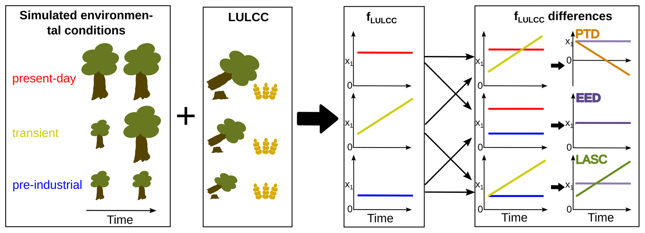
Figure 1 Illustration of the different f_LULCC estimations and their differences. The altered sizes of trees (box 1) indicate that vegetation responds to the historical trends in environmental conditions (such as increased CO₂ levels and global warming). Historically and globally, environmental changes led to an increase in land C stocks, therefore present-day environmental conditions are associated with taller trees in our scheme. When a LULCC occurs that reduces C stocks (box 2) the higher C stocks will cause a higher f_LULCC (box 3: red line (present-day) higher than blue line (pre-industrial); yellow line (transient) increasing with time). The f_LULCC is derived by subtracting the net biome productivity from a simulation without LULCCs from one with LULCCs. Additionally, the different f_LULCC estimations can be compared to each other (box 4): the loss of additional sink capacity (LASC; green line; Eq. 4), environmental equilibrium difference (EED; purple line; Eq. 5), and “present-day” vs. “transient” environmental conditions difference (PTD; orange line; Eq. 6).

Assuming constant environmental conditions or C densities over time is clearly unrealistic and requires an arbitrary decision on the time period to determine these variables' values. On the other hand, as discussed, the lost sinks in DGVM-based f_LULCC under realistic, transient environmental conditions do not correspond to observable fluxes. This poses the question about a proper definition of f_LULCC for a robust and realistic attribution that is valid across time and space. It needs to be decided whether the LASC should be included or excluded (as argued, e.g. in Gasser and Ciais, 2013; Gasser et al., 2020) as part of the f_LULCC and consequently be counted towards the terrestrial C sink or not. The urgent need to address this question is underlined by the fact that past LULCCs are estimated to have committed a reduction in the potential global C sink of 80–150 PgC by 2100, which depending on the scenario, translates into a share of ∼70 % of the total global f_LULCC (Strassmann et al., 2008).

This study aims to strengthen the basis for a decision on how to define the f_LULCC, in particular with respect to the ability of different approaches to resolve the LASC, and thus is a guide on the future role of DGVMs in f_LULCC attribution. To this end, we present analyses concerning the relevance of different assumptions on environmental conditions, for which the recent extended set of TRENDY DGVM simulations was performed. In particular, our study (1) discusses and quantifies three DGVM-derived f_LULCC (under pre-industrial, transient, and present-day environmental conditions) and bookkeeping estimates in conjunction with their inherent differences on global scale, (2) quantifies the temporal evolution of the differences in DGVM-derived f_LULCC estimates for 18 regions, (3) differentiates between climate- and CO₂-induced f_LULCC components as derived by DGVMs, and (4) aims to approach a spatio-temporally homogenized attribution of the f_LULCC as derived by models.

2 Data and methods

This study is based on an ensemble of TRENDY v8 models (http://sites.exeter.ac.uk/trendy/, last access: 5 April 2021) that ran simulations with and without LULCC for the period 1700–2018 (used in the GCB2019 to quantify the f_LULCC uncertainty and to estimate the natural terrestrial C sink; Friedlingstein et al., 2019). It is ensured that all models have reached (1) a steady state after spinup (offset in global NBP < 0.1 PgC yr⁻¹ and drift < 0.05 PgC yr⁻¹ per century), (2) a net land flux over the 1990s within 90 % confidence of constraints by global atmospheric and oceanic observations, and (3) f_LULCC as a C source to the atmosphere over the 1990s (Friedlingstein et al., 2019).

2.1 Models and simulations

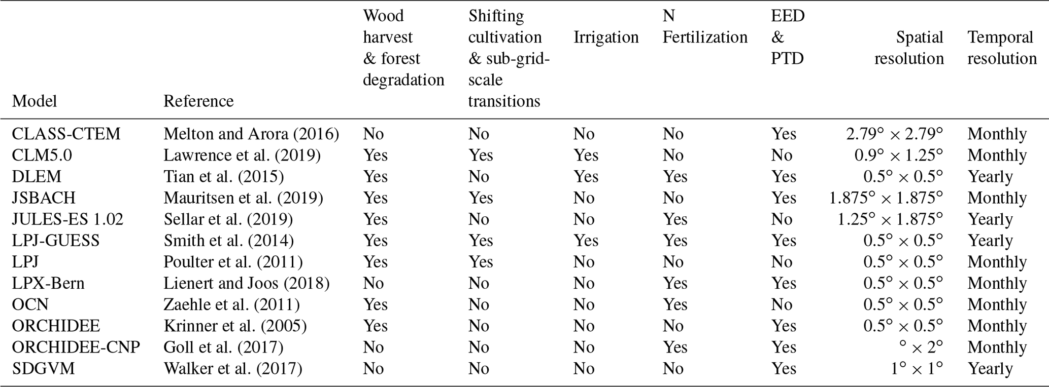
We use 12 TRENDY v8 DGVMs that provide gridded output of NBP with and without LULCCs under both transient (historically observed) and pre-industrial (constant) environmental conditions (called S0, S2, S3, S4 in the TRENDY v8 protocol; see Table 1) to calculate the LASC on a regional level (see Table 2 for a comparison of the model output and relevant processes included in the DGVMs; additional information can be found in Table A1 in Friedlingstein et al., 2019). Note, for SDGVM, model output from TRENDY v9 was used due to erroneous merging of land cover and LULCC datasets in earlier versions that caused a C loss over the period ∼1900–1970 mainly in semi-arid regions. For eight models that provided simulations under constant present-day environmental forcing (S5, S6), the f_LULCC was also calculated under present-day environmental conditions. All TRENDY v8 simulations were started in 1700 after C stocks reached equilibrium with environmental conditions in the models to enable reproducible results with minimized initialization effects for the analysed time period starting in 1850. This implies two separate spinups: one for simulations conducted under present-day environmental conditions (S5, S6) and one for those starting from or keeping pre-industrial conditions (all others).

Table 1 Overview of the simulations used in our study comprising transient (observed historical evolution), pre-industrial or present-day (constant) forcing for environmental conditions (such as climate and atmospheric CO₂ concentrations), and transient or fixed pre-industrial land use and cover distribution (with an additional description of their purpose of use). For the underlying forcing data and protocol, refer to Friedlingstein et al. (2019). All runs were performed within the TRENDY v8 efforts for the GCB2019.

Melton and Arora (2016)Lawrence et al. (2019)Tian et al. (2015)Mauritsen et al. (2019)Sellar et al. (2019)Smith et al. (2014)Poulter et al. (2011)Lienert and Joos (2018)Zaehle et al. (2011)Krinner et al. (2005)Goll et al. (2017)Walker et al. (2017)

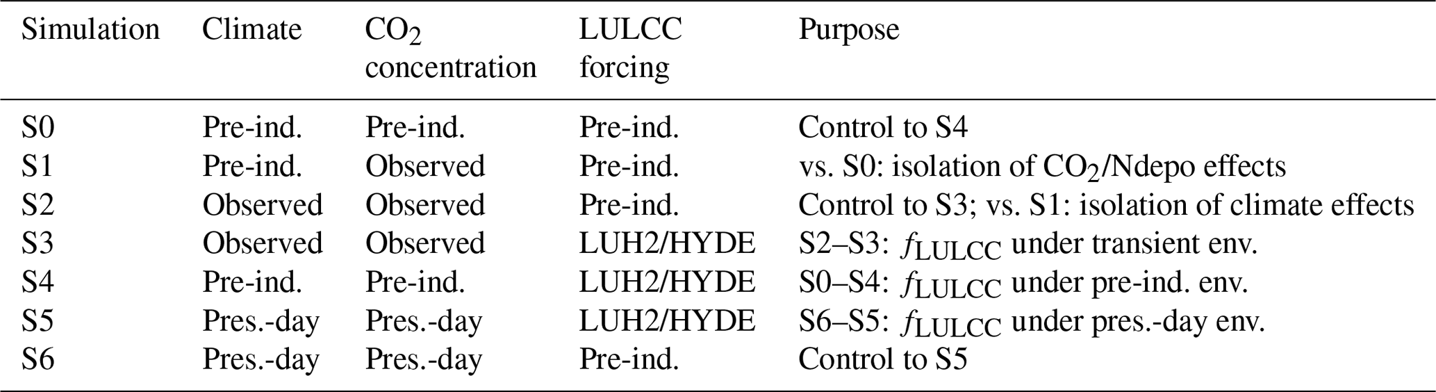
Table 2 Overview of the TRENDY v8 DGVM model output provided and used in this study and of selected processes included that are relevant for the f_LULCC. Also indicated is if a plausible derivation of the environmental equilibrium difference (EED, Eq. 5 and Sect. 2.2.1) and “present-day” vs. “transient” environmental conditions difference (PTD, Eq. 6 and Sect. 2.2.1) was possible.

The DGVM simulations with observed transient environmental conditions used observation-based temperature, precipitation, and incoming surface radiation data at 0.5×0.5 degree spatial resolution of the Climatic Research Unit (CRU) and Japanese Reanalysis (JRA; Friedlingstein et al., 2019; Harris et al., 2014). Annual time series of global atmospheric CO₂ concentrations for 1700–2018 was derived from ice core data (before 1958; Joos and Spahni, 2008) merged with National Oceanic and Atmospheric Administration (NOAA) data (from 1958 onward; Dlugokencky and Tans, 2020). Models used land use change data from the History Database of the Global Environment (HYDE), which provides annual, half-degree, fractional data on cropland, rangeland, and pasture areas based on annual statistics of the Food and Agriculture Organization of the United Nations (FAO; Klein Goldewijk et al., 2017; Goldewijk et al., 2017) or the updated harmonized land use change data (LUH2; Hurtt et al., 2011, 2020). While HYDE agricultural areas are used in LUH2, the main difference lies in LUH2 additionally adding wood harvest from the Global Forest Resources Assessments of the FAO and sub-grid-scale (“gross”) transitions to capture shifting cultivation in the tropics.

For pre-industrial simulations, the CO₂ concentration and LULCC data from 1700 were applied, and climate was derived by recycling the mean and variability from 1901–1920. For present-day simulations, the CO₂ concentrations from 2018 were taken as constant, and climate was derived by recycling the mean and variability from 1999–2018.

2.2 Data processing

2.2.1 Three alternative f_LULCC estimates and their differences

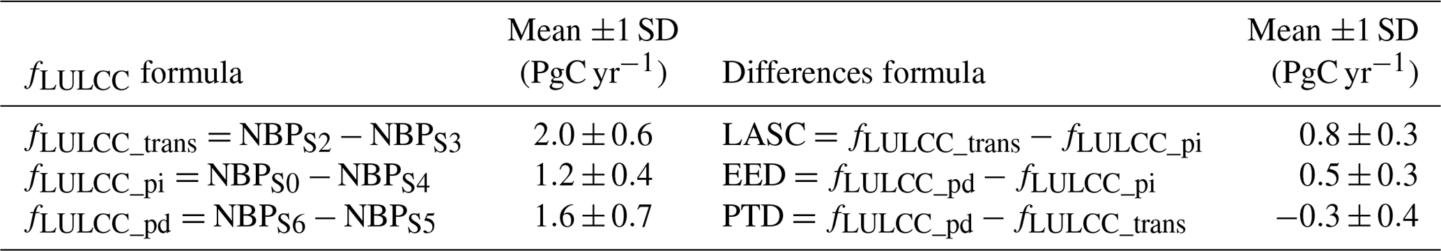
We infer the three different DGVM-based f_LULCCs each from the differences in NBP of a simulation with and one without LULCCs (Eqs. 1 to 3; see Table 1 for description of simulations S0 to S6 and Fig. 1 for a schematic of resulting carbon fluxes). For example, we derive the f_LULCC under transient environmental conditions by subtracting NBP in S3 from NBP in S2 (Eq. 1). Using yearly aggregated NBP values, the f_LULCC is derived for each DGVM, time step, and grid cell under transient (subscript trans), constant pre-industrial (pi), and constant present-day (pd) environmental conditions from the TRENDY v8 simulations as follows:

$$\begin{array}{}\text{(1)}& {\displaystyle }& {\displaystyle }{f}_{\mathrm{LULCC}\mathrm{\_}\mathrm{trans}}={\mathrm{NBP}}_{\mathrm{S}\mathrm{2}}-{\mathrm{NBP}}_{\mathrm{S}\mathrm{3}}\text{(2)}& {\displaystyle }& {\displaystyle }{f}_{\mathrm{LULCC}\mathrm{\_}\mathrm{pi}}={\mathrm{NBP}}_{\mathrm{S}\mathrm{0}}-{\mathrm{NBP}}_{\mathrm{S}\mathrm{4}}\text{(3)}& {\displaystyle }& {\displaystyle }{f}_{\mathrm{LULCC}\mathrm{\_}\mathrm{pd}}={\mathrm{NBP}}_{\mathrm{S}\mathrm{6}}-{\mathrm{NBP}}_{\mathrm{S}\mathrm{5}}.\end{array}$$

Here, a lower NBP in the simulation including LULCC (S3 to S5) compared to the one excluding LULCC (control, S0 to S2 and S6) represents a net flux of CO₂ out of the terrestrial biosphere into the atmosphere (emissions) due to LULCC causing reduced C uptake or C losses. Conversely, a higher NBP in the simulation including LULCCs relates to a net flux from the atmosphere into the biosphere due to LULCCs that enhanced C uptake.

As outlined in the introduction, the derivation of f_{LULCC_trans} (Eq. 1; definition as used for uncertainty assessment in the GCB2019; Friedlingstein et al., 2019) inherently includes the LASC. The LASC represents theoretical emissions resulting from transient alterations of environmental conditions since the beginning of the simulation runs (historical changes in climate and atmospheric CO₂ and N deposition, the latter for models including N-cycling) and, thus, can be quantified with reference to f_{LULCC_pi}, fluxes that would have occurred if pre-industrial environmental conditions prevailed during and after the time LULCCs occurred (Eq. 4; e.g. Strassmann et al., 2008; Pongratz et al., 2009; Gitz and Ciais, 2003; Gasser et al., 2020).

$$\begin{array}{}\text{(4)}& \begin{array}{rl}\mathrm{LASC}& =f_{\mathrm{LULCC}\mathrm{\_}\mathrm{trans}}-f_{\mathrm{LULCC}\mathrm{\_}\mathrm{pi}}=\left({\mathrm{NBP}}_{\mathrm{S}\mathrm{2}}-{\mathrm{NBP}}_{\mathrm{S}\mathrm{3}}\right)\\ & -\left({\mathrm{NBP}}_{\mathrm{S}\mathrm{0}}-{\mathrm{NBP}}_{\mathrm{S}\mathrm{4}}\right)\end{array}\end{array}$$

The LASC hinders comparison of f_{LULCC_trans} with flux estimates based on present-day environmental conditions (f_{LULCC_pd}). Per definition, the latter represent the closest approximation of bookkeeping fluxes and recent C density observations via DGVMs. Therefore, we compare f_{LULCC_trans} and f_{LULCC_pd} to determine times and regions that are most sensitive to the differences introduced when DGVM-derived f_{LULCC_trans} is jointly used with bookkeeping estimates, as in the GCB2019. We call this the “present-day” vs. “transient” environmental conditions difference (PTD) and derive it according to Eq. (5):

$$\begin{array}{}\text{(5)}& \begin{array}{rl}\mathrm{PTD}& =f_{\mathrm{LULCC}\mathrm{\_}\mathrm{pd}}-f_{\mathrm{LULCC}\mathrm{\_}\mathrm{trans}}=\left({\mathrm{NBP}}_{\mathrm{S}\mathrm{6}}-{\mathrm{NBP}}_{\mathrm{S}\mathrm{5}}\right)\\ & -\left({\mathrm{NBP}}_{\mathrm{S}\mathrm{2}}-{\mathrm{NBP}}_{\mathrm{S}\mathrm{3}}\right).\end{array}\end{array}$$

It is not clear even at global scale if the PTD is negative or positive. On one hand, f_{LULCC_pd} can be higher than f_{LULCC_trans} because C stocks had been brought into equilibrium with present-day conditions during spinup, i.e. ecosystems had time to equilibrate with high CO₂ levels, implying more biomass and higher soil C stocks being affected by – historically prevalent – deforestation. On the other hand, the LASC accumulates over time (Sect. 1 and Fig. 1 for illustration) and therefore f_{LULCC_trans} could become larger than f_{LULCC_pd}. This difference is assumed to be particularly pronounced in former forested areas under beneficial environmental conditions over the past where LULCCs happened early, as the LASC could accumulate for a long time (high sensitivity of forest productivity to rising CO₂ in DGVMs; compare, e.g. Peng et al., 2014).

The LASC and PTD add up to the difference of f_{LULCC_pd} and f_{LULCC_pi}. The latter two are derived under constant environmental forcing, meaning that both are indifferent to long-term environmental trends (see Fig. 1 for illustration). However, the choice of the time period from which constant environmental conditions are taken is arbitrary. Nonetheless, comparison of these two simulations is interesting, as they span the minimum and maximum range of assumptions on environmental conditions that would make sense to consider under typical industrial-era simulations. Up to now, no comparison of f_{LULCC_pi} with f_{LULCC_pd} exists in the literature, which is why we derive their difference and introduce it as the environmental equilibrium difference (EED; Eq. 6):

$$\begin{array}{}\text{(6)}& \begin{array}{rl}\mathrm{EED}& =f_{\mathrm{LULCC}\mathrm{\_}\mathrm{pd}}-f_{\mathrm{LULCC}\mathrm{\_}\mathrm{pi}}=\left({\mathrm{NBP}}_{\mathrm{S}\mathrm{6}}-{\mathrm{NBP}}_{\mathrm{S}\mathrm{5}}\right)\\ & -\left({\mathrm{NBP}}_{\mathrm{S}\mathrm{0}}-{\mathrm{NBP}}_{\mathrm{S}\mathrm{4}}\right).\end{array}\end{array}$$

Twelve TRENDY v8 DGVMs were compared regarding the f_{LULCC_pi}, f_{LULCC_trans}, and LASC. The f_{LULCC_pd} (and consequently the EED and PTD) could not be derived for CLM5.0, JULES, LPJ, and OCN (no S5 and S6 simulation; eight models). A discussion of the performance of individual models can be found in the appendix (Sect. A1).

To gain insight into the spatial trends and drivers of the three DGVM-derived f_LULCC estimates and their differences, a regional analysis was conducted based on the REgional Carbon Cycle Assessment and Processes, Phase 2 (RECCAP2) regions defined in Tian et al. (2019) and shown in Fig. A2. Since all global and regional analyses were performed based on the original model output, the RECCAP2 map was regridded to each model's native resolution using largest area fraction remapping (to compare globally summed NBP in this study and in the GCB2019, refer to Fig. A13). Note, for grid point-wise comparison, all model output was regridded to 720×360 grid boxes using first-order conservative remapping (Jones, 1999).

Due to high interannual NBP variability, the resulting regional and global f_LULCC estimates were smoothed by a Savitzky–Golay filter using 5 % of the spatially summed annual data points (16 years). Savitzky–Golay smoothing was applied to preserve peak heights and widths, which are known to be removed by other smoothing practices such as moving averages.

All data pre-processing and statistical analysis were performed using Climate Data Operator software (CDO, v1.9.3; Schulzweida, 2019), netCDF Operators (NCO, v4.7.7; Rew et al., 1997), and raster- (v2.8-4; Hijmans and van Etten, 2014), ncdf4- (v1.16.1; Pierce, 2019), matrixStats- (v0.56.0; Bengtsson et al., 2020), and pracma- (v2.2.9; Borchers, 2019) packages of the CRAN R universe (v3.4.4; R Core Team, 2018).

2.2.2 Relative climate- vs. CO₂-induced f_LULCC components

Climate-change-related environmental alterations might increase or decrease NBP over time (compare Sect. 1) and, thus, cause higher or lower f_{LULCC_trans} and f_{LULCC_pd} compared to f_{LULCC_pi} or bookkeeping estimates. While increasing CO₂ concentrations are assumed to generally increase C stocks across the globe, alterations by other environmental changes (mainly precipitation- and temperature-related) are more heterogeneous. To gain knowledge about the underlying environmental drivers for changes in f_LULCC quantities, this study aims to differentiate between their climate- and CO₂-induced components. We approximate them using S1 and S2 simulations, which differ only with respect to inclusion of climatic changes (Table 1). These simulations do not include transient LULCCs and can therefore not directly be used to estimate the climate vs. CO₂ related alteration of the f_LULCC. However, assuming that the proportions of climate- vs. CO₂-induced C stock changes (we use the total C stocks in vegetation and soil, cTot) translate linearly into the CO₂-induced f_{LULCC_trans} component at each grid cell ($f_{\mathrm{LULCC}\mathrm{\_}{\mathrm{CO}}_{\mathrm{2}}}$), we derive the latter based on the ratio of cTot in S1 to S2 simulations (Eq. 7). The validity of this approach is supported by the f_LULCC in many regions, correlating well with biomass stocks across models (Li et al., 2017). Thus, although LULCCs may affect C stocks with different strengths – based on the extent, practice, and local ecosystem conditions (including C stock distribution) – it seems appropriate to assume that the f_LULCC is not independent from the environmental driver of C stock changes.

$$\begin{array}{}\text{(7)}& f_{\mathrm{LULCC}\mathrm{\_}{\mathrm{CO}}_{\mathrm{2}}}=f_{\mathrm{LULCC}\mathrm{\_}\mathrm{trans}}\times \left({\mathrm{cTot}}_{\mathrm{S}\mathrm{1}}/{\mathrm{cTot}}_{\mathrm{S}\mathrm{2}}\right)\end{array}$$

Ratios of cTot were derived based on the annual averages in the last decade of the simulation period across all models (2009–2018). Due to generally increased differences and ratios of cTot_S1 and cTot_S2 over the simulated period (Fig. A1), our $f_{\mathrm{LULCC}\mathrm{\_}{\mathrm{CO}}_{\mathrm{2}}}$ provides the maximum possible contribution of CO₂-induced change in the f_LULCC. Here we note that interacting effects of elevated CO₂ concentrations and temperature or precipitation on biomass productivity (observed under experimental setups; e.g. Obermeier et al., 2017) might obscure this attribution (Lombardozzi et al., 2018). Nevertheless, the assessment of the relative contribution through this approach seams valid as no significant interactions between these influencing factors on C stocks were observed within the TRENDY ensemble (Fernández-Martínez et al., 2019) nor within a fully coupled single model investigation (Devaraju et al., 2016).

C stocks from LPX-Bern and CLM5.0 were excluded from derivation of multi-model mean C stocks due to very high values, in particular in high latitudes of the Northern Hemisphere due to the inclusion of peatlands (for LPX-Bern, compare Spahni et al., 2013). C stock outliers smaller than 0 were excluded.

As no TRENDY v8 control simulation with pre-industrial LULCC and CO₂ concentrations and observed (transient) climate exists, we indirectly assess the climate-only f_LULCC component (f_{LULCC_Climate}; Eq. 8). Note that by subtracting $f_{\mathrm{LULCC}\mathrm{\_}{\mathrm{CO}}_{\mathrm{2}}}$ from the total f_LULCC to derive the climate-only flux shares, this approach assumes zero synergies between the effects of CO₂ concentrations and climatic changes on NBP in the DGVMs. While in reality they may be substantial (e.g. increased water use efficiency due to stomatal closure under elevated CO₂), it is beyond the possibilities of the available data to quantitatively assess these synergistic effects.

$$\begin{array}{}\text{(8)}& \begin{array}{rl}{f}_{\mathrm{LULCC}\mathrm{\_}\mathrm{Climate}}& =f_{\mathrm{LULCC}\mathrm{\_}\mathrm{trans}}-f_{\mathrm{LULCC}\mathrm{\_}{\mathrm{CO}}_{\mathrm{2}}}\\ & =f_{\mathrm{LULCC}\mathrm{\_}\mathrm{trans}}-f_{\mathrm{LULCC}\mathrm{\_}\mathrm{trans}}\\ & \times \left({\mathrm{cTot}}_{\mathrm{S}\mathrm{1}}/{\mathrm{cTot}}_{\mathrm{S}\mathrm{2}}\right)\end{array}\end{array}$$

Note that within the TRENDY v8 simulations, pre-industrial and present-day climate forcing is defined as a recycling of climates in the earliest decades of the 20th and 21st century, respectively (see Sect. 1). Consequently, the climate change impact derived in this study roughly represents the last hundred years, which seems a reasonable approximation of the history, given that proxy-based temperature reconstructions, for example, cannot detect a warming earlier than the beginning of 20th century (Hegerl et al., 2019).

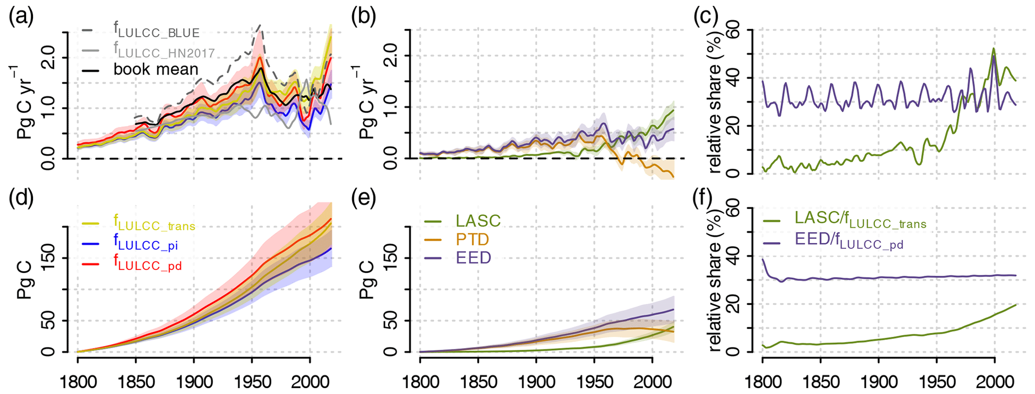
Figure 2 Multi-model means of smoothed global annual values (a–c) and cumulative sums (d–f) of f_LULCC estimates (a, d), the loss of additional sink capacity (LASC; b, c), the “present-day” vs. “transient” environmental conditions difference (PTD; b, c), the environmental equilibrium difference (EED; b, c), and the relative contributions of the LASC and EED to f_{LULCC_trans} and f_{LULCC_pd} respectively (c, f) from 1800 to 2018. Additionally, the f_LULCC from the bookkeeping models BLUE and H&N2017 as well as their average is plotted (data for GCB2019; not shown for cumulative sums due to shorter data coverage). For absolute values from this study, the 95 % confidence intervals are also shown. See Figs. 3 and 4 for an individual model's results for f_LULCC estimates and their differences, respectively.

3 Results and discussion

3.1 Differences in f_LULCC estimates on the global scale

A general overview of most recent annual and cumulative estimates of f_LULCC shows that our estimates are in good agreement with published estimates (Friedlingstein et al., 2019; Gasser et al., 2020; Tables 3 to A3). Slight differences (<0.1 PgC yr⁻¹) between f_{LULCC_trans} derived in this study and the DGVM-derived GCB2019 estimates are attributable to the fact that we used only a subset (n=12) of the models analysed within the GCB2019 (n=15) in order to consistently use the same models where possible. Additionally, the inclusion of TRENDY v9 model output for SDGVM (for the reasons, refer to Sect. 2) caused, for example, a lower LASC of 0.8 PgC yr⁻¹ for 2009–2018 in this study (0.84 PgC yr⁻¹ with two decimal places) as compared to consistently using TRENDY v8 output, where the resulting LASC (usually rounded to one decimal place) is 0.9 PgC yr⁻¹ due to rounding of 0.85 PgC yr⁻¹.

Table 3 Overview of global annual f_LULCC estimates and their differences (loss of additional sink capacity, LASC; “present-day” vs. “transient” environmental conditions difference, PTD; environmental equilibrium difference, EED) for the time period 2009–2018. Mean and standard deviation refer to the DGVM model ensemble.

As expected (Sect. 1), f_{LULCC_pd} is the DGVM-based f_LULCC estimate that is most similar to the bookkeeping mean in the GCB2019 when compared over multiple years. The LASC explains the relatively high difference of f_{LULCC_trans} to the bookkeeping estimates in the GCB2019 and by Gasser et al. (2020) since bookkeeping models, by their nature, do not include the LASC. Lower LASC estimates in the GCB2019 compared to our findings are based on an early version of the reduced-complexity Earth system model OSCAR, which was constrained to the land sink without LULCC perturbation as estimated by DGVMs (Gasser and Ciais, 2013; Gasser et al., 2017). Later revised OSCAR versions constrained to the net land flux as residual from fossil emissions, atmospheric growth, and the ocean sink yielded higher LASC estimates (that were more similar to our study; Gasser et al., 2020).

A closer look at the historical evolution of the three global f_LULCC estimates reveals similarities, despite the substantial differences in their annual and cumulative quantities shown before. In particular, trends remain similar over time, with an increase since the start of the simulations peaking in the 1950s and again at the end of the simulation (Figs. 2a and 3a–c). Congruent patterns of f_{LULCC_pd} and bookkeeping mean values highlight the validity of our approach to investigate regions that are most sensitive towards the choice of transient DGVM- vs. bookkeeping-based estimates (Figs. 2a and 3c). A widely congruent trend was also found across the DGVMs, while their absolute values partly differ strongly across models, for example global f_{LULCC_trans} and f_{LULCC_pi} from OCN is largely higher than in the other models, with estimates more than twice as large as the one from ORCHIDEE and LPX-Bern (Fig. 3a and b and Sect. A1 for a discussion of individual model results). Note, a high internal climate variability translates into a high interannual variability in NBP and consequently a high variability of f_LULCC estimates (Figs. 3, 5, and A13) and of their respective differences (Figs. 4 and 6). For the differences in f_LULCC estimates, some artefacts might additionally arise due to the comparison of simulations with different forcing cycles (e.g. on the global scale with periodic fluctuations in annual relative shares of the EED to f_{LULCC_pd} in Fig. 2c and, on a regional scale, in Figs. 6 and A4 to A6 with pronounced oscillations in some regions).

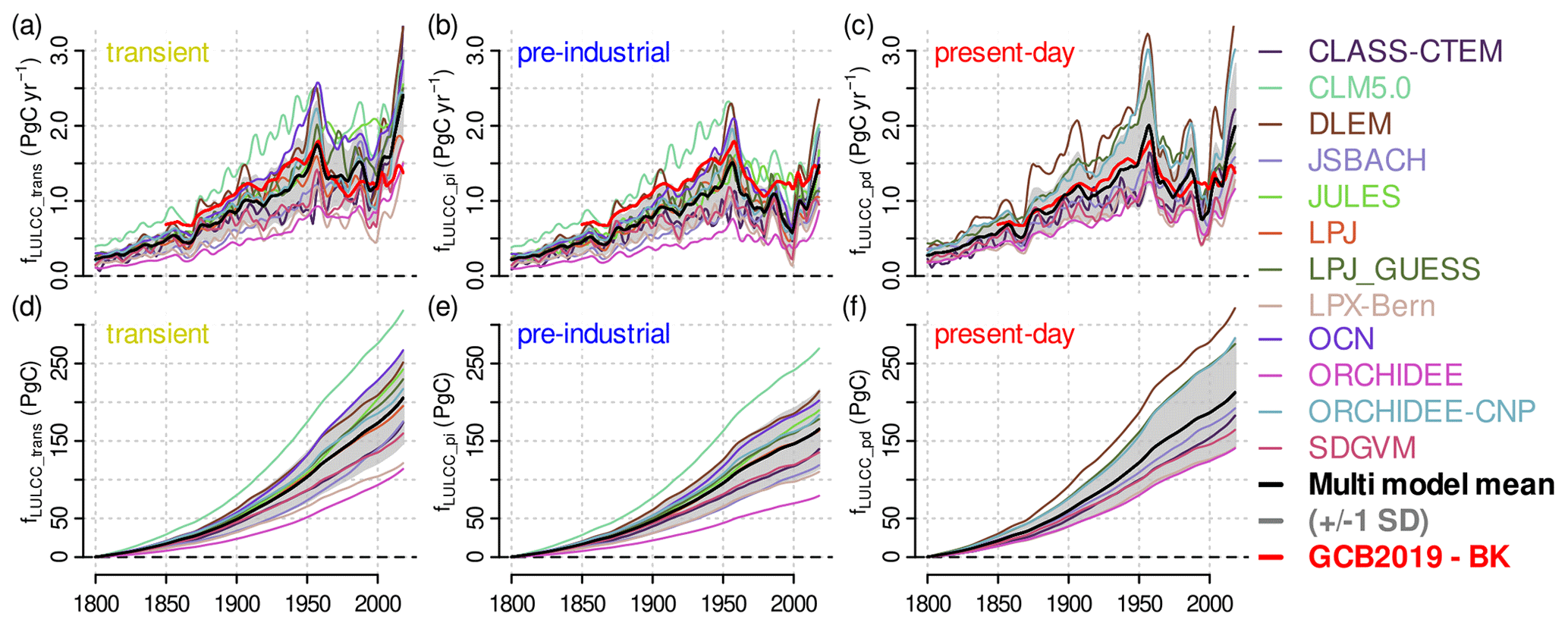
Figure 3 Smoothed global annual means (a–c) and cumulative sums(d–f) of f_{LULCC_trans} (a, d), f_{LULCC_pi} (b, e), and f_{LULCC_pd} (c, f) for the investigated DGVMs from 1800 to 2018. For the derivation formulas refer to Eqs. (1) to (3) and for discussion of individual models refer to Sect. A1. f_{LULCC_pd} was not derived for CLM5.0, JULES, LPJ, and OCN (compare Table 2). For comparison, we also included the GCB2019 bookkeeping mean (same values in all panels).

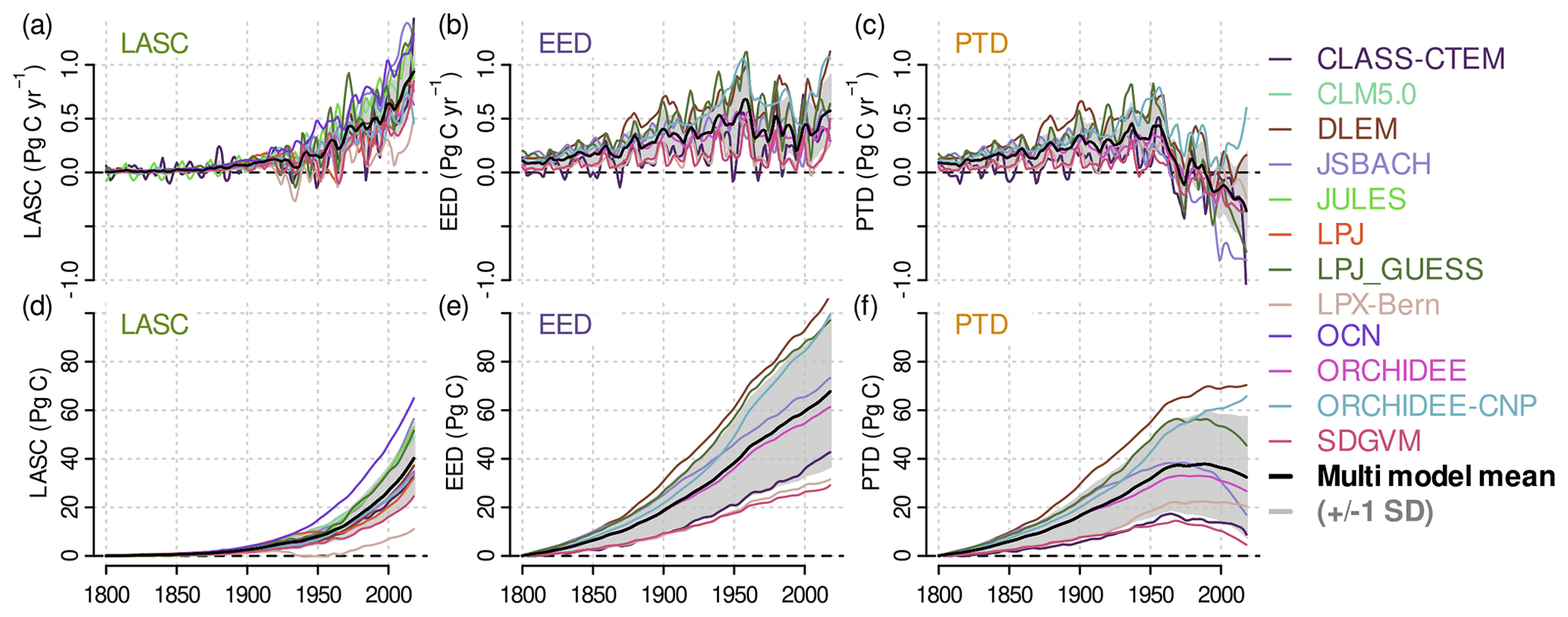
Figure 4 Smoothed global annual values (a–c) and their cumulative sums (d–f) of the differences in f_LULCC estimates for the investigated DGVMs from 1800 to 2018: loss of additional sink capacity (LASC; a, d), environmental equilibrium difference (EED; b, e), and “present-day” vs. “transient” environmental conditions difference in the f_LULCC (PTD; c, f). For the derivation formulas refer to Eqs. (4) to (6) and for discussion of individual models refer to Sect. A1. The EED and PTD were not derived for CLM5.0, JULES, LPJ, and OCN (compare Table 2).

Figure 5 Region-wise smoothed multi-model mean annual f_{LULCC_trans} (a, b), f_{LULCC_pi} (c, d), and f_{LULCC_pd} (e, f) from 1800 to 2018, derived according to Eqs. (1) to (3). For discussion of individual models refer to Sect. A1 and Figs. A7 to A9. f_{LULCC_pd} was not derived for CLM5.0, JULES, LPJ, and OCN (Table 2).

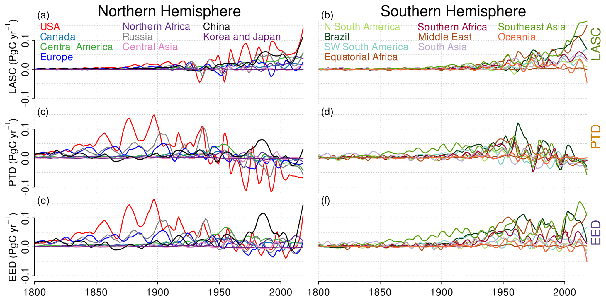
Figure 6 Region-wise smoothed multi-model mean annual loss of additional sink capacity (LASC; a, b), difference between the f_LULCC under present-day and pre-industrial environmental conditions (environmental equilibrium difference, EED; c, d), and “present-day” vs. “transient” environmental conditions difference in the f_LULCC (PTD; e, f) from 1800 to 2018, derived according to Eqs. (4) to (6). For discussion of individual models refer to Sect. A1 and Figs. A4 to A6 and Figs. A10 to A12. The PTD was not derived for CLM5.0, JULES, LPJ, and OCN (Table 2).

Throughout the 19th century, hardly any differences are found between f_{LULCC_trans} and f_{LULCC_pi} (i.e. a LASC around 0; Figs. 2a–d and 4a and d) indicating a negligible impact from environmental changes (i.e. CO₂ concentrations and climate). Accordingly, the constantly higher and faster increasing annual and cumulative f_{LULCC_pd} (concomitantly the PTD and EED; Figs. 2a, b, d, e and 4b, c, e, f) can be explained by higher C stocks due to their equilibration to present-day conditions rather than pre-industrial ones (see Fig. 8 for historical C stock changes in the transient simulation). Similarly, the higher bookkeeping mean values compared to f_{LULCC_trans} and f_{LULCC_pi} up to the 1950s are attributable to their use of recent inventory-based C densities (Figs. 2a and 3a, b).

By the end of 19th century, annual and cumulative f_{LULCC_trans} estimates start to exceed f_{LULCC_pi} estimates (Fig. 2a and d). This can be related to higher C stocks due to an accelerated atmospheric CO₂ increase where LULCCs leading to net loss in C stocks occurred (e.g. deforestation). Additionally, the aforementioned nature of the LASC, as a synergistic effect of changes in environmental conditions and any LULCC that occurred since the start of the simulation, comes into play. In general, beneficial environmental alterations for C sequestration widely increased the potential C stocks (Fig. 8) and, thus, the LASC steadily increased (Figs. 2b, e and 4a, d), reaching about ∼40 % in recent annual and ∼20 % in cumulative contributions to f_{LULCC_trans} (Fig. 2c and f). Despite this LASC increase, global annual and cumulative f_{LULCC_pd} estimates still increase faster than the other estimates during this period (first half of 20th century; the EED and PTD continue to increase), indicating that synergistic effects of LULCCs with higher C stocks under present-day conditions still outweigh the amount of additional emissions accumulated by the LASC (an EED greater than the LASC is also represented by positive PTD values; Figs. 2b and 4c).

In the 1950s, global peaks in annual f_{LULCC_pi} and f_{LULCC_pd} estimates were observed (Figs. 2a and 3b, c). As these estimates neglect transient environmental conditions and do not include the LASC, these peaks simply relate to a strongly increased amount of LULCCs depleting C stocks, in particular on C-dense land where historic environmental changes would have highly increased the potential C stocks (Fig. 8). The latter is highlighted by the simultaneous peak in the EED, which in essence is the intersection of LULCCs with the difference in standing biomass and actual soil C stocks due to altered environmental conditions over the last hundred years (under pre-industrial vs. present-day environmental conditions; compare Fig. 2a with Fig. 2b and Sect. 2.2.2).

The LASC becomes particularly evident after the 1950s (Figs. 2b and 4a, d) when the global peak of converted C stocks by LULCCs was passed and a reduced amount of LULCCs decreasing C stocks caused strongly decreased annual f_{LULCC_pi} and f_{LULCC_pd} (and EED) estimates. By contrast, f_{LULCC_trans} decreased only slightly, as the LASC grows largely due to a combination of large areas that have been transformed from natural vegetation to fast-turnover agricultural areas (not least during the 1950s peak in global LULCCs) and CO₂ levels accelerating their increase (Fig. A1). This accelerating increase of the LASC causes annual f_{LULCC_trans} estimates to surpass those of f_{LULCC_pd} starting, for the multi-model mean, around 1960. The PTD, as a consequence, becomes small then negative (a small temporal lag is caused by the reduced subset of models used for PTD derivation). Around the same time, the LASC becomes larger than the EED, indicating that the foregone sinks by LULCCs outweigh the flux changes upon LULCCs under present-day vs. pre-industrial environmental conditions post 1950 (with presumably higher estimates from DGVMs as compared to bookkeeping models). These changing differences in f_LULCC estimates over time highlight how sensitive the choice of the f_LULCC definition is to the considered timescales even on the global scale (with a relative contribution of the EED to f_{LULCC_pd} of ∼35 %, Fig. 2c and f).

3.2 Differences in f_LULCC estimates on regional level

Where does the LASC occur, and which regions are most sensitive towards the investigated DGVM-based f_LULCC definitions (under constant pre-industrial and present-day or transient environmental conditions)? Compared to smoothed global curves, where signals average out, it must be expected that synergistic effects of C stock alterations in combination with the occurrence and timing of LULCCs cause higher differences between the three f_LULCC estimations on a regional scale. We assess these differences on a spatio-temporally explicit level using the RECCAP2 regions (Fig. A2) and show regional annual values of multi-model mean f_{LULCC_trans}, f_{LULCC_pi}, and f_{LULCC_pd} (Fig. 5) and of their differences LASC, PTD, and EED (Fig. 6; cumulative estimates are shown in Figs. A10 to A12). Global maps of the cumulative sums and most recent annual mean estimates are shown in Figs. 9 and 10; individual model results are discussed in Sect. A1 and shown in Figs. A4 to A12.

A large sensitivity of cumulative f_LULCC towards choice of pre-industrial vs. present-day environmental forcing is found in vast stretches across the globe: EED cumulated >8 PgC in the USA (mainly eastern parts), Brazil (mainly southern parts), and Southeast Asia; >5 PgC in Russia, China, equatorial Africa, and southern Africa; and >2 PgC in Europe (mainly eastern parts), southwest South America and South Asia from 1800 until 2018 (Figs. 10e and A12). Strikingly, the last decade saw the tropics become more dominant in positive EED than other regions due to recent clearings (Figs. 5 and 10f). All these reflect particularly forested areas where LULCCs caused the highest f_LULCC quantities (Figs. 5 and 9a, c, e; compare increasing deviation of linear model from 1:1 line with higher values) due to the conversion of land with high NBP where positive changes in potential C stocks between 1800 and 2018 occurred (Fig. 8).

Conversely, very distinct regions of negative cumulative EED in Central Europe reflect increased C storage and, thus, a relatively stronger negative f_{LULCC_pd} due to early and widespread reforestation causing increased C uptake (Fig. 9e). Such a strong C uptake due to reforestation also caused globally widespread negative EED values in the last decade (Fig. 10f; with hotspots in northeastern Brazil, southern Africa and the Eurasian steppe zone), while the poor representation of recent large-scale reforestation programmes with a concomitantly increased C sink in China (Lu et al., 2018; Chen et al., 2019) in the LUH2 data prevents the EED (and also f_LULCC estimates) from becoming negative in this region.

Regions that were only a little affected by LULCCs, for example remote rainforests, hardly show up in the EED. The pattern of the EED is thus dominated by the pattern of LULCC with variations due to ecosystem sensitivity (namely in NBP) to environmental conditions (see Fig. 7). This shows that the choice of pre-industrial vs. present-day environmental conditions can play a substantial role in the regional f_LULCC attribution.

Figure 7 Multi-model means of the relative share of cumulative environmental equilibrium difference (EED) to f_{LULCC_pd} from 1800 to 2018. Grid points with cumulative f_{LULCC_pd}<0.5 and $>-\mathrm{0.5}$ were excluded from mapping.

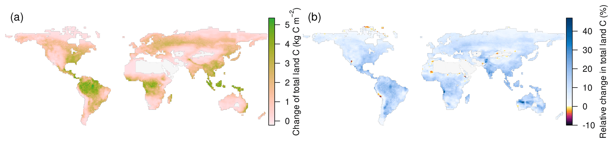
Figure 8 Multi-model means of absolute (a) and relative (b) changes in total carbon stocks (cTot; soil and vegetation carbon combined) from ∼1800 (average from 1800–1809) until today (average from 2009–2018) in the S2 simulation (including all environmental changes) within the vegetation extent of 1700. Grid points < 1 kgC m⁻² cTot in the later period were excluded.

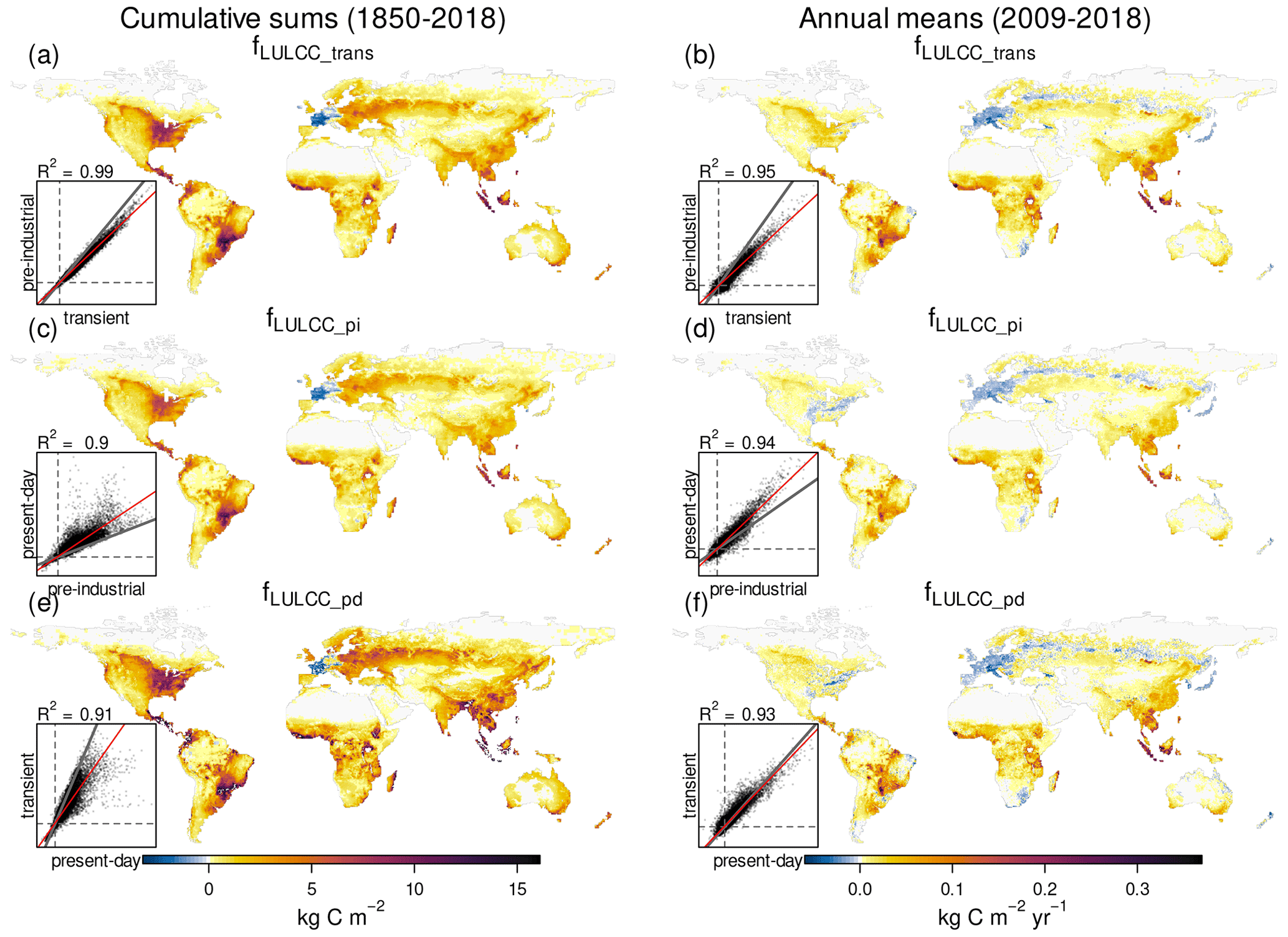
Figure 9 Cumulative sums from 1850 onward (a, c, e) and annual means for 2009–2018 (b, d, f) of f_{LULCC_trans} (a, b), f_{LULCC_pi} (c, d), and f_{LULCC_pd} (e, f) averaged across the models. Additionally, correlation plots between the pixel-wise estimations are shown; here, the grey line represents the 1:1 line, the dashed grey lines depict zero lines, and the red line shows a fitted linear model. f_{LULCC_pd} was not derived for CLM5.0, JULES, LPJ, and OCN models (compare Table 2).

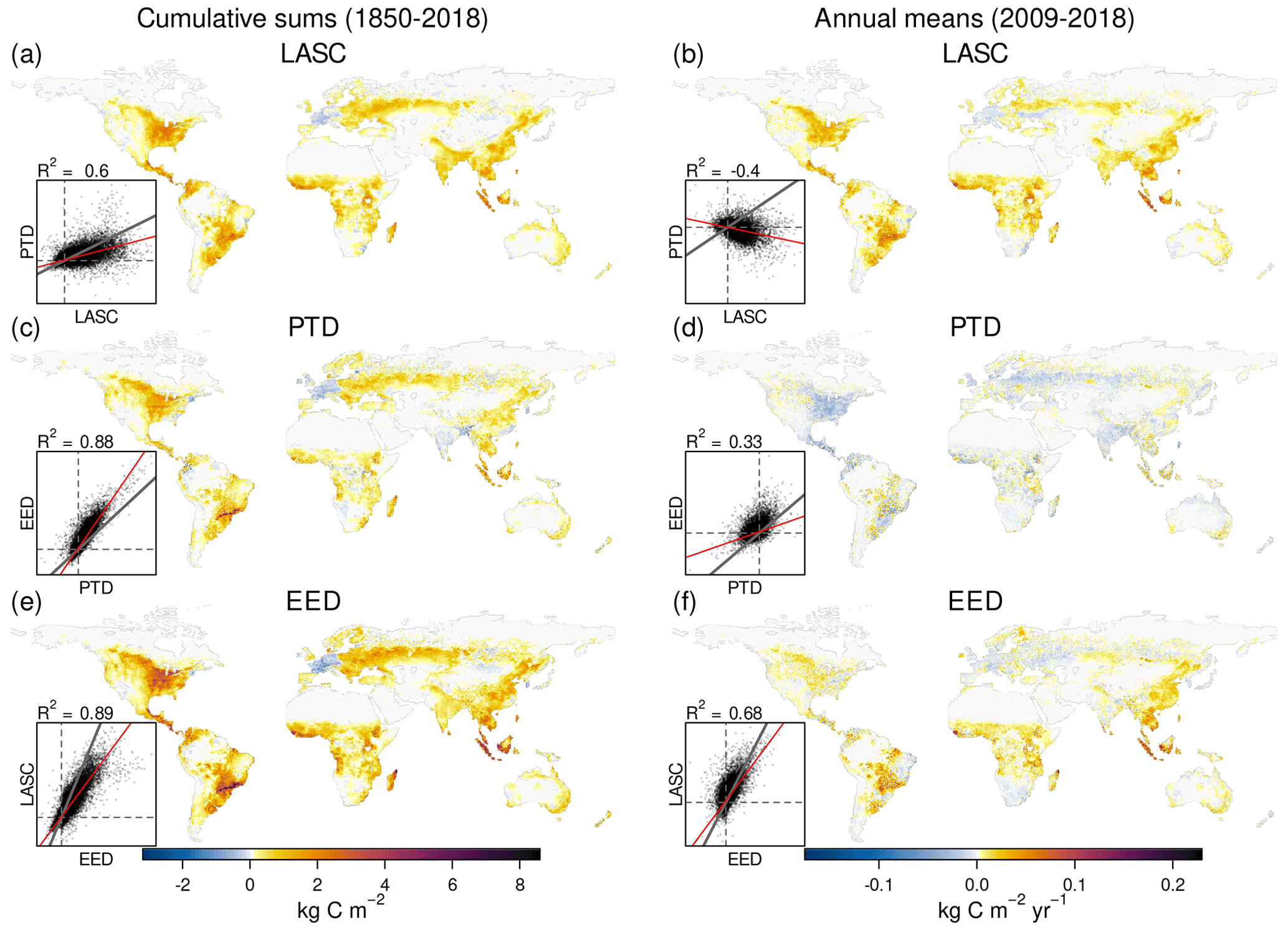
Figure 10 Cumulative sums from 1850 onward (a, c, e) and annual means for 2009–2018 (b, d, f) of the loss of additional sink capacity (LASC; a, b), the “present-day” vs. “transient” environmental conditions difference (PTD; c, d) and the environmental equilibrium difference (EED; e, f) averaged across the models. Additionally, correlation plots between the different pixel-wise estimations are shown; here, the grey line represents the 1:1 line, the dashed grey lines depict zero lines, and the red line shows a fitted linear model. The EED and PTD were not derived for CLM5.0, JULES, LPJ, and OCN models (see Table 2).

As seen for the global estimates, the approach to derive the f_LULCC under transient environmental conditions introduces even more complexity, as it includes the LASC and strongly depends on the timing of LULCCs. Along these lines, the PTD undergoes a trend reversal with widely negative values in the most recent period in many regions (Figs. 6c, d and 10d), which we discuss in detail in the next section.

3.2.1 Regions of positive loss of additional sink capacity – a lost carbon sink?

Not surprisingly, the regions of the largest LASC values are related to the EED (compare Figs. 6 and 10a, e, with strong correlation between the LASC and EED shown in the latter) and similar values to the PTD (Fig. 10c) are in line with the cumulative LASC amounting to about half of the EED globally (Fig. 2e). But marked differences in patterns exist, which reflect that although the LASC is driven by environmental differences, just as the EED, it differs in causing legacy fluxes on any area cleared in the past via the reference simulation seeing the potential vegetation within its pre-industrial extent. These differences are pronounced in the last decade (Figs. 6 and 10b, d, f): regions, in particular forested regions, that were cleared between 1700 and the middle of the 20th century (when the accelerated CO₂ increase causes a strongly accumulating LASC) and stayed non-forested continuously create emissions during later times when the LASC is included and cause the LASC to be larger than the EED (i.e. a negative PTD).

While the EED is more relevant than the LASC for cumulative industrial-era emissions (change of sign in correlation with inlet Fig. 10e compared to Fig. 10f), the accumulating LASC heavily alters recent f_LULCC estimates; Fig. 10b shows which regions would be attributed much higher emissions when the LASC is included in the f_LULCC definition. Aggregated time series for the RECCAP2 regions reveal that the LASC started to increase in  ∼1850 in the USA, Russia, and Southeast and South Asia and in ∼1900 in southwest South and Central America and southern Africa (Figs. 6a, b and A4). It then becomes even more pronounced ∼1950 in Brazil, equatorial Africa and China, with the latter two and Southeast Asia showing a particular strong increase after 2000 (Figs. 6a, b, 10b and A4). Overall, the LASC accumulated to more than 4 PgC in the USA, Brazil, equatorial Africa, and Southeast Asia, and to 2–4 PgC in China, Russia,southwest South and Central America, southern Africa, and South Asia (Figs. 10a and A10). As stated above, these high cumulative and annual LASC estimates mainly result from an initial high forest coverage and subsequent C losses in particular on areas where higher C stocks resulted from environmental changes over time (Sect. 3.4 and Fig. 8). Due to the different start of organized human agriculture, the forest clearings in the USA (mid-19th century, with an early LASC initiation) though on forests with comparably low C stocks (Fig. A3) have caused similar cumulative sums compared to the much later widespread LULCCs (beginning of 20th century) in Brazil, equatorial Africa, China, and Southeast Asia (Fig. A10) due to rapidly increasing and pronounced higher vegetation C stocks in these regions (with strong response to CO₂ increase).

The widely negative PTD values across the globe for the period 2009–2018 indicate that the LASC causes recent f_LULCC estimates from the current DGVM approach (under transient conditions) to be higher compared to bookkeeping estimates (which are similar to f_{LULCC_pd}). However, small areas exist where the EED remains larger than the LASC (i.e. positive PTD values) for the recent decade; here, more recent LULCCs caused an even shorter period for the LASC to accumulate in the tropics (mainly Brazil, Tanzania, Indonesia), sub-tropics (eastern China, southern Australia), and in the transition zones from temperate to boreal zone (Scandinavia, Russia). These regions would likely be attributed higher emissions by bookkeeping approaches than by f_{LULCC_trans} from DGVMs. This highlights another difficulty especially in the regional f_LULCC attribution: as the LASC accumulates emissions caused by past LULCCs, recent LULCCs are given less weight in relative terms. This also applies to recent LULCCs reducing atmospheric CO₂ such as reforestation, which cannot quickly compensate for past LULCC in approaches including the LASC, while they could in f_{LULCC_pi} and f_{LULCC_pd} estimates.

3.2.2 Regions of negative loss of additional sink capacity – a gained carbon sink?

While it has been shown above that the LASC is strong and positive in many regions, adding globally almost 1 PgC yr⁻¹ to the recent annual f_LULCC, the LASC may be negative in some regions. Negative cumulative LASC estimates from 1800 onward are seen for wide areas of Europe, small areas in Brazil (eastern parts) and southern Africa (eastern parts), and with lower quantities spread over Canada, Russia, and China (Figs. 10a and A10). Negative annual LASC estimates for the period 2009–2018 are observed in the same regions but are more widespread in Brazil and southern Africa and have striking negative values in the Ukraine (Figs. 6, 10b, and A4). These negative LASC estimates can mainly be explained by LULCCs beneficial for C stocks (e.g. reforestation) on areas that experienced beneficial environmental conditions afterwards, with a negative cumulative LASC indicating that the positive effects of LULCCs on the C stocks outweighed the effects of, mostly earlier, LULCCs that decreased C stocks. Note that this depends on the time LULCCs occurred, as the LASC accumulation periods differ in their duration as well as the underlying transient environmental conditions. Along these lines, the strong negative cumulative and annual LASC estimates across France, Germany, and Italy result from widespread reforestation after 1700, but also from the fact that the pre-industrial land use already had low forest coverage due to pre-1700 deforestation (Klein Goldewijk et al., 2017), despite belonging to the forest biome. Most recent negative LASC values in the Ukraine can be linked to recultivation of post-Soviet abandoned agricultural land, in particular in the Steppe zone (Smaliychuk et al., 2016). However, a negative LASC may also represent a negative climate change impact on C stocks (e.g. reduced precipitation) in areas where LULCCs decreasing C stocks happened (e.g. the Iberian Peninsula and eastern parts of South Africa).

The areas with a negative LASC are consequently attributed lower f_LULCC emissions to the atmosphere when the LASC is included in the calculation. If political reporting were based on DGVM-based f_{LULCC_trans} estimates of the GCB instead of a bookkeeping approach, these regions would “profit” the most (be attributed less emissions). In other areas of widespread reforestation, most recent annual LASC estimates remain positive albeit decreasing, depending on how much the LASC has accumulated before as synergy between the timing of LULCCs and later environmental C stock alterations. Here, a negative PTD indicates that the LASC accumulated more than the difference of the actual fluxes upon detrimental LULCCs under transient vs. present-day conditions (e.g. due to a long accumulation period) or that beneficial LULCCs caused smaller negative emissions in f_{LULCC_trans} as compared to f_{LULCC_pd}.

Comparing the different f_LULCC estimates over time and across space, previous discussion has shown that the choice of method to derive the f_LULCC strongly impacts the estimated quantities. The effects of the interaction of the environmental forcing with the timing of the actual LULCC is particularly pronounced for estimates under transient environmental forcing and where NBP was strongly altered by environmental changes.

3.3 Relative climate- and CO₂-induced f_{LULCC_trans} components

As discussed (Sect. 2.2.2), patterns of CO₂ and climate changes may have very different effects on the f_LULCC across the globe. The mean simulated global vegetation C stock increased by ∼23 % from 664 to 815 PgC from 1800 until today in both the S1 and S2 simulation (which by protocol exclude effects from LULCCs; see Figs. 8 and A3 for maps and Fig. A1b for global estimates). The mean simulated global soil C stock increased from 1494 to 1569 PgC (∼5 %) in S1 and to 1553 PgC (∼4 %) in the S2 simulation (see Fig. A1c). In line with the more pronounced soil C stock increase in the S1 simulation (excluding climatic changes), the general increase in cTot can mainly be attributed to an altered CO₂ exposure under rising atmospheric CO₂ (Lal, 2008). However, although climate change (here roughly the last 100 years due to model assumptions; compare Sect. 2.2.2) induces lower changes in C stocks on global scale, it has high impact on local and regional scale.

Climate change increased cTot mainly through vegetation changes in the mid- and high latitudes, which can be explained by increased temperatures leading to longer growing seasons, boreal expansion of biomes (Peng et al., 2014; Piao et al., 2019), and increased precipitation in some regions (e.g. CMIP5 precipitation changes of last century in Becker et al., 2013; van den Besselaar et al., 2013). Negative climate change impacts on C stocks are mainly found across the tropics for vegetation and in most regions of the world for soil C. These negative climate-induced stock alterations likely relate to reduced precipitation amounts (e.g. Ren et al., 2013; van den Besselaar et al., 2013) with an increased frequency and intensity of droughts (e.g. Bastos et al., 2020), increased temperatures further increasing the vapour pressure deficit (potentially enhancing transpirational water losses) and increasing soil respiration and mineralization processes (reducing soil C stocks; Lal, 2008; Crowther et al., 2016; Davidson and Janssens, 2006), and increased disturbances such as forest fires (Bowman et al., 2009; Archibald et al., 2018). The apparent dipoles in climate-induced vegetation and total C stock alterations in the USA and over Europe are most likely triggered by environmental changes during the 20th century with reduced stocks in the western USA and southern Europe where precipitation decreased (and droughts happen more frequent) and higher stocks in the eastern USA where precipitation widely increased (and droughts get less likely; e.g. Peterson et al., 2013; van den Besselaar et al., 2013) and northern Europe due to global- warming-induced longer growing seasons (e.g. Keenan et al., 2014; O'Sullivan et al., 2020) .

In line with the homogeneously altered C stocks due to increased CO₂, spatial patterns of the CO₂-induced f_LULCC component ($f_{\mathrm{LULCC}\mathrm{\_}{\mathrm{CO}}_{\mathrm{2}}}$) widely reflect f_{LULCC_trans} and thus LULCC activities, while the climate-induced f_LULCC component is much more heterogeneously spread (Sect. 2.2.2 and Fig. 11). The highest $f_{\mathrm{LULCC}\mathrm{\_}{\mathrm{CO}}_{\mathrm{2}}}$ occurs in the tropics and in the mid-latitudes, where changes in vegetation C dominate the C pool changes and vast areas have been transformed by LULCCs that decreased C stocks (Figs. A3 and 11a, b). Negative $f_{\mathrm{LULCC}\mathrm{\_}{\mathrm{CO}}_{\mathrm{2}}}$ estimates are mainly found where f_{LULCC_trans} is also negative and can be explained by agricultural abandonment and/or reforestation (for small areas in the northeast USA and northeast Brazil and wide areas in Europe, parts of Russia, Georgia, Korea, Japan, and South Africa).

Figure 11 Cumulative sums from 1850–2018 (a, c, e) and annual means for 2009–2018 (b, d, f) of $f_{\mathrm{LULCC}\mathrm{\_}{\mathrm{CO}}_{\mathrm{2}}}$ (a, b), f_{LULCC_Climate} (c, d), and percentage change in f_{LULCC_trans} due to climate change only (e, f; $\mathrm{100}\times (f_{\mathrm{LULCC}\mathrm{\_}\mathrm{trans}}-f_{\mathrm{LULCC}\mathrm{\_}{\mathrm{CO}}_{\mathrm{2}}})/f_{\mathrm{LULCC}\mathrm{\_}\mathrm{trans}}$). Grid boxes < 1 kgC m⁻² total C stock excluded from mapping.

Although comparably low in absolute values, climate-change-induced alterations in the f_LULCC are much more heterogeneously spread over the globe and range from −23 % to +28 % with particular high alterations on areas with comparably low C stocks (compare Figs. 11c–f and A3). A reduced f_{LULCC_Climate} occurs where vegetation C is also reduced due to climate, mainly in the tropics and sub-tropics with particular hotspots in northeastern Brazil, the Mediterranean region, southern and eastern Africa, China, southern Asia, southwestern Australia, and Central America (the latter, despite higher vegetation C), and in the temperate zone in western USA and Mongolia. In contrast to this climate-induced f_LULCC reduction, climate strongly increased f_LULCC in particular in the colder environments of higher latitudes and altitudes where higher C stocks resulted from climate change (Sect. 2.2.2).

4 Proposal for a standard f_LULCC estimation

The previous sections have shown for the first time that f_LULCC patterns depend not only on the timing of occurrence and type of LULCCs, but also on the simulated time period and the assumptions on environmental conditions (with spatially very diverse effects from climate alterations). From a policy standpoint and disregarding considerations from the natural land sink perspective, these results highlight the need for a f_LULCC estimate that is comparable over time and across space. For example, including the LASC in f_LULCC estimates may be perceived as appropriate because LULCCs could have destroyed or created vegetation with long C turnover (e.g. deforestation or reforestation) leading to decreased or increased C sinks (while current f_LULCC reporting neglects such foregone sinks). However, including the LASC implies attributing fluxes to a region's emission budget that are partly a fate of history; particularly in the temperate regions, LULCCs detrimental to C stocks historically happened earlier compared to LULCCs increasing C stocks. Thus, the committed emissions included in the LASC often have longer accumulation periods for detrimental as compared to beneficial LULCCs whose accumulation periods are more likely to be cut off at the simulation end (2018 in the GCB2019). The accumulation periods may be further altered if, over the historic period, various LULCCs occurred on the same area. This is further complicated because environmental changes over the historic period modified the LASC with a widely accelerated accumulation rate in later periods due to higher and faster increasing CO₂ concentrations but very heterogeneously spread alterations by climatic changes. Thus, even for the same LULCC with the same accumulation duration, the LASC will be different depending on the timing and location of the LULCC.

To circumvent these issues, as could be desired in the political context, one could derive f_LULCC and the LASC based on simulations forced with the cycled climate and CO₂ conditions that occurred during the actual LULCC event. However, this would still result in differing accumulation periods and varying environmental conditions during and following a LULCC event. While the influence of the latter could be reduced using cycled pre-industrial or present-day environmental forcings, these neglect transient C stock changes. To consider the LASC but counteract spatial heterogeneity in f_LULCC differences resulting from synergistic effects of environmental conditions and the timing of LULCCs, one could derive the f_LULCC and LASC from a defined reference period that is independent of the actual time that LULCCs occurred and shares the same reference conditions. For example, the f_LULCC and LASC could always be modelled for the second half of the 21st century, as here the environmental C stock changes have been amplified due to the accelerating increase of atmospheric CO₂ concentrations (alternative start times are of course conceivable). By using such a reference period, the LASC could also be fully captured for most recent LULCCs (regardless of whether they act positive or negative on C stocks) and foregone sinks would be more equally counted (same length of accumulation period with similar environmental changes). Along these lines, it may be considered to calculate such an adapted LASC based on CO₂-only simulations as in this case the impact of humans is more homogeneously distributed, while the spatially heterogeneous climate impact on f_LULCCs, determined foremost by action outside the location of LULCCs, causes a questionable attribution of the regional f_LULCC when compared across the globe (without even considering externalized f_LULCCs; e.g. due to remote market demand of food and timber; Lambin and Meyfroidt, 2011; Meyfroidt et al., 2013). To detach f_LULCC estimates from the timing of LULCCs and the spatially heterogeneous climate evolution, we argue to address the delineation of an adapted LASC in future studies, where, in particular, the reference to calculate the LASC should further be investigated. Such methodology could limit the f_LULCC to locally determined factors (namely LULCCs) and reduce the dependence on the timing of LULCCs while still reflecting the foregone C sink capacity by human intervention.

5 Conclusions

Accurate quantification of the net carbon flux from land use and land cover changes (f_LULCC) is essential, foremost to project carbon (C) cycle dynamics and estimate the strength of negative CO₂ emission technologies. However, the f_LULCC can only be estimated by models – typically bookkeeping or dynamic global vegetation models (DGVMs) – and requires decisions on how to account for the effects of environmental changes. We show that these decisions have major consequences for flux attribution, particularly at the regional scale because C stocks evolve very heterogeneously in both space and time. DGVM estimates under present-day environmental forcing most closely resembled bookkeeping estimates (used in the annual global carbon budgets, GCBs) and are generally higher compared to the f_LULCC under pre-industrial environmental conditions. This environmental equilibrium difference (EED; accounting for ∼35 % of global f_LULCC when using present-day C stocks) is caused by higher C stocks, mainly in response to increased present-day atmospheric CO₂ and only to a smaller extent by climatic changes. The EED becomes negative in some regions, mainly due to environmental conditions decreasing C stocks (e.g. increased frequency and intensity of droughts and reduced precipitation). In the GCB, cumulative bookkeeping f_LULCC estimates are jointly published with DGVM-derived uncertainties under transient environmental conditions, which we show implies pronounced regional differences (named “present-day” vs. “transient” environmental conditions difference; PTD), strongly depending on the timing and placement of land use and land cover changes. We explain PTD values mainly by the loss of additional sink capacity (LASC), emissions due to destroyed C uptake potential that are only captured by the transient DGVM approach. In our multi-model mean for 2009–2018, a LASC of 0.8±0.3 PgC yr⁻¹ accounts for ∼40 % of recent global f_LULCC estimates of 2.0±0.6 PgC yr⁻¹ (under transient conditions).

The LASC causes regionally strongly increased transient f_LULCC (>0.1 PgC yr⁻¹) where LULCCs detrimental to C stocks, such as deforestation, happened early within the simulated period (long accumulation period for lost potential C uptake; foremost in the USA) or later on areas with strong positive C stock response to environmental changes (e.g. in Brazil, Southeast Asia, and equatorial Africa). The LASC from deforestation is unaccounted for in nations that deforested prior to the beginning of the accounting period (e.g. widespread deforestation in Europe). Further, in many of these cases the LASC is negative and transient f_LULCC is strongly decreased due to early reforestation on previously deforested land where re-established forest carbon stocks profited from environmental change (e.g. widespread in Europe). Within the political context, if environmental effects on C sink capacity are to be accounted for in regional budgets (requiring DGVMs for the assessment) we argue for a consistent method that includes the LASC and emphasize that care must be taken in choosing the beginning of the accounting period. As LASC values derived by the approach taken so far in the GCB are widely independent of locally determined environmental changes (rather, they depend on globally determined climatic changes) and strongly dependent on accumulation periods (defined by the timing of LULCCs and the end year of the simulations), we argue for a f_LULCC attribution that is more robust against choices of environmental drivers and accumulation period by using an adapted LASC, for example, based on a defined common reference period and homogeneously altered environmental conditions (such as only being driven by CO₂ alterations).

Appendix A

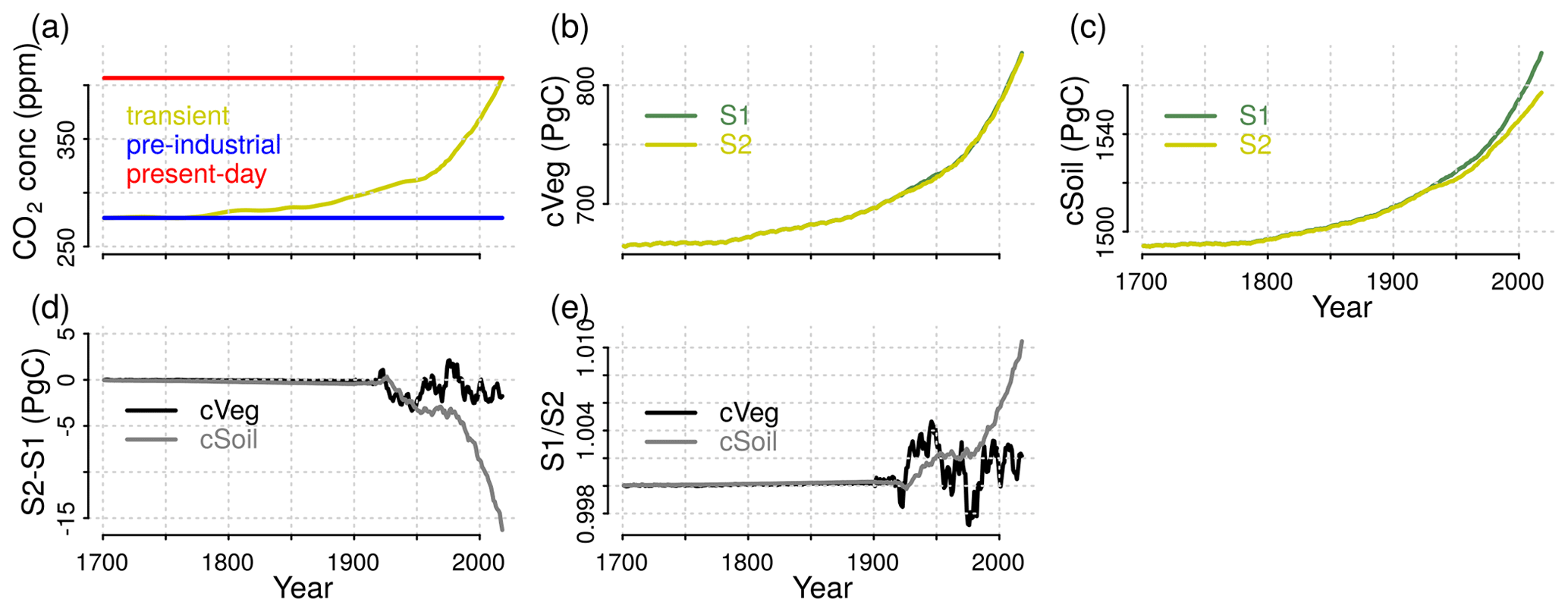
Figure A1 Global forcings of annual CO₂ fields and ensemble mean C stocks in vegetation and soil of the S1 (pre-industrial climate and transient CO₂) and S2 (transient climate and CO₂) simulation runs. Additionally, the differences and ratios in S1 and S2 C stocks in vegetation and soil are plotted.

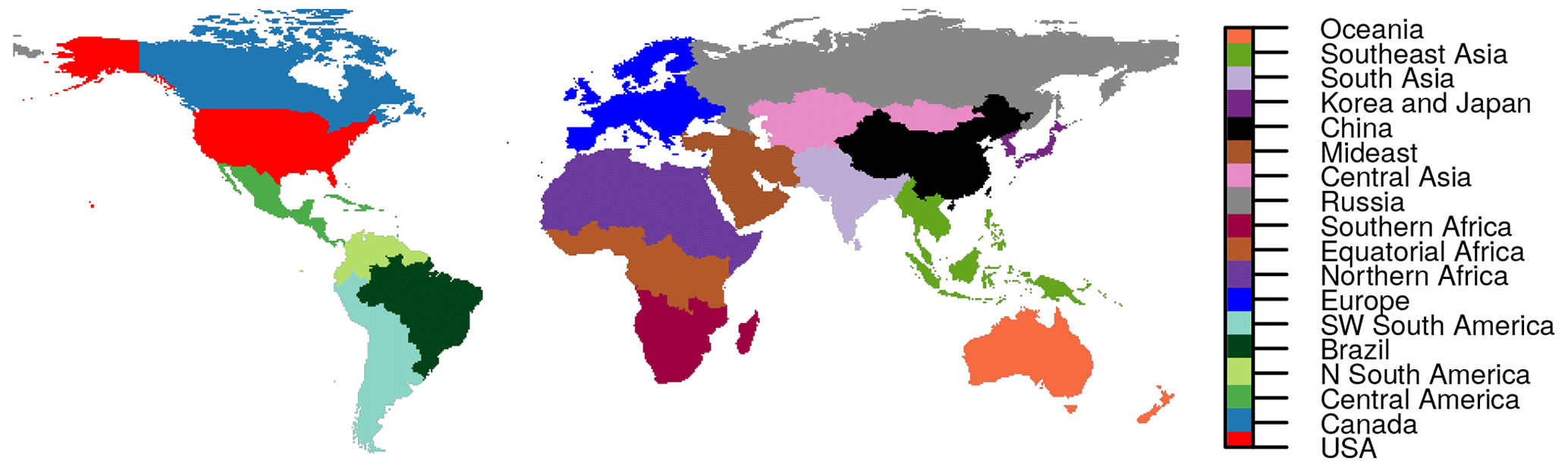
Figure A2 REgional Carbon Cycle Assessment and Processes', Phase 2 (RECCAP2) regions as defined in Tian et al. (2019).

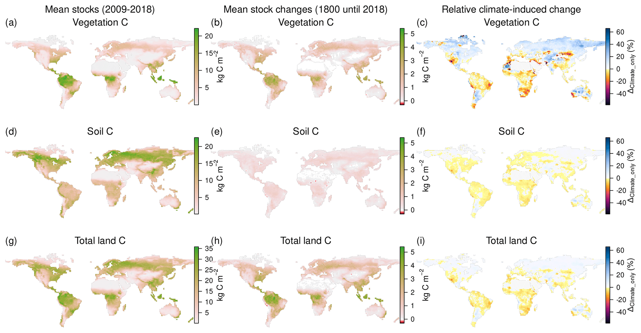
Figure A3 Ensemble mean C stocks from 2009–2018 in the S2 simulation (a, d, g; observed environmental conditions and pre-industrial land use and land cover), mean C stock changes between 1800 and 2018 (b, e, h), and their climate-induced percentage changes (c, f, i, $\mathrm{100}\times (\mathrm{S}\mathrm{2}-\mathrm{S}\mathrm{1})/\mathrm{S}\mathrm{2})$ of vegetation (a–c; for relative change, values $<-\mathrm{60}$ % were set to −60 %), soils (d–f), and their totals (g–i). The relative climate-induced changes indicate additional (blueish) and reduced (reddish) stocks due to historic climate change (grid points <1 kgC m⁻² total C stock excluded).

Figure A4 Region-wise smoothed annual loss of additional sink capacity (LASC) in the investigated DGVMs from 1800 to 2018, derived according to Eq. (4). For discussion of individual models refer to Sect. A1. The last two panels show regional ensemble means on a uniform scale.

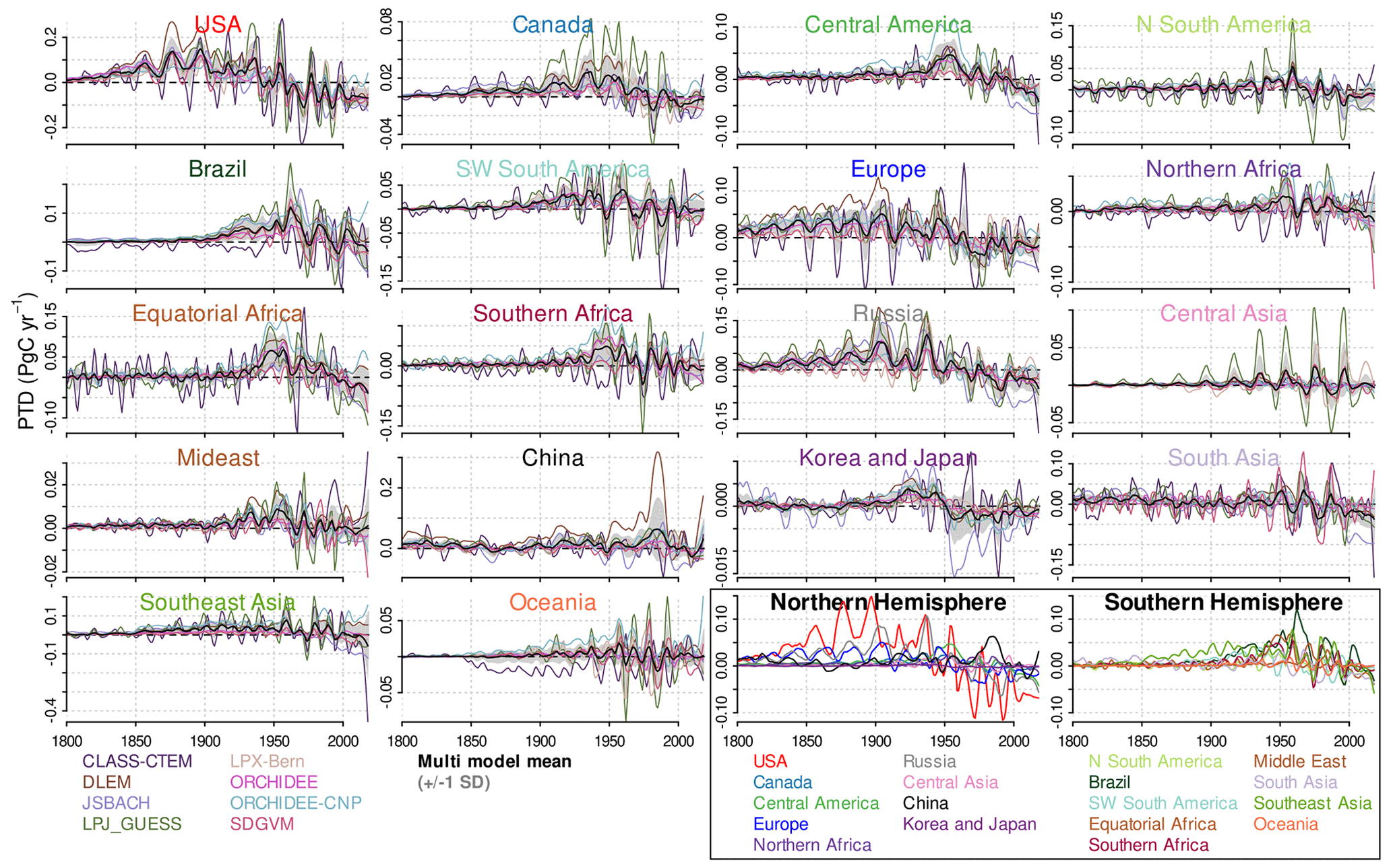
Figure A5 Region-wise smoothed annual “present-day” vs. “transient” environmental conditions difference in the f_LULCC (PTD) in the used models from 1800 to 2018, derived according to Eq. (5). For a discussion of individual models refer to Sect. A1. The PTD was not derived for CLM5.0, JULES, LPJ, and OCN (compare Table 2). The last two panels show regional ensemble means on a uniform scale.

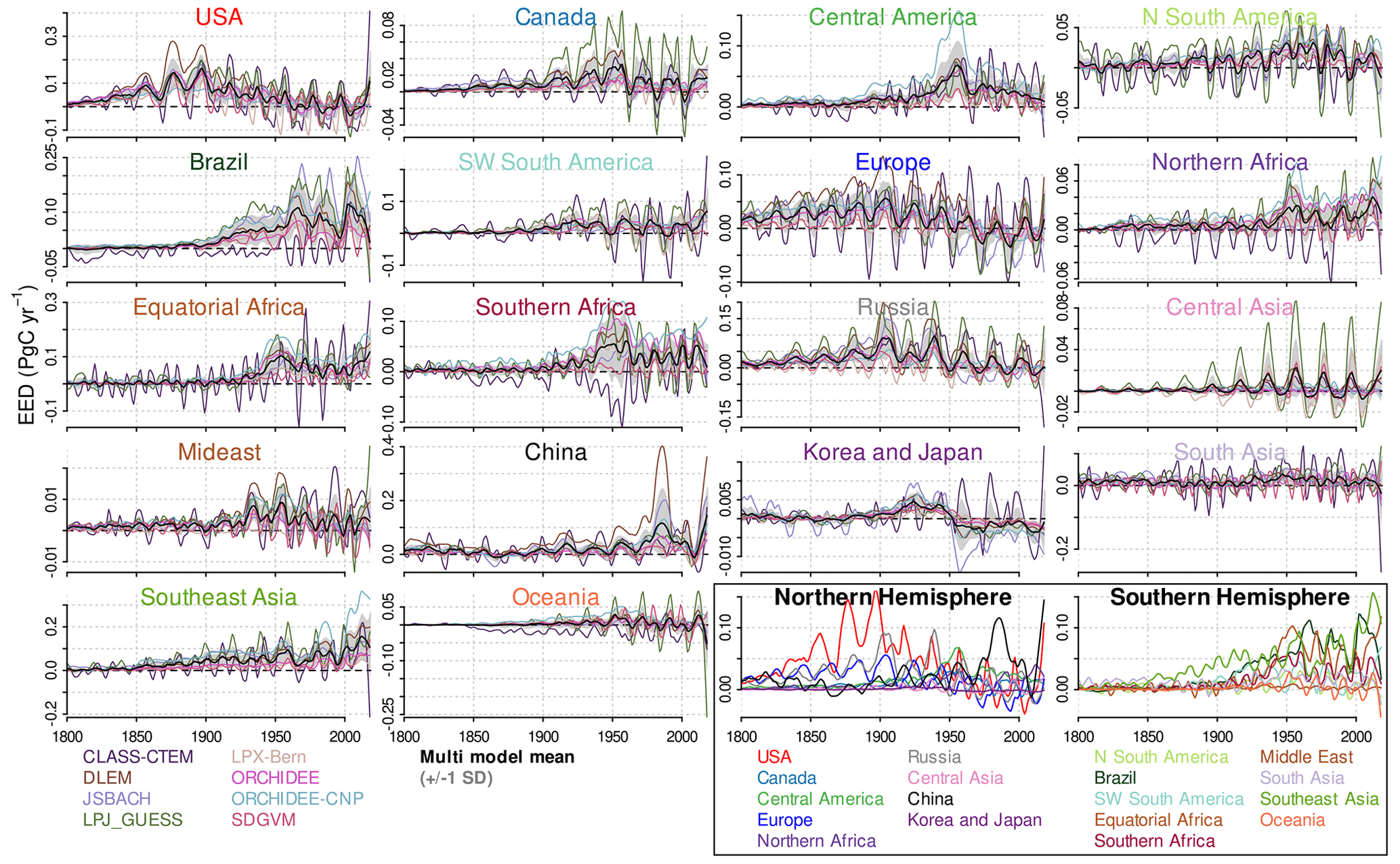
Figure A6 Region-wise smoothed annual difference between the f_LULCC under present-day and pre-industrial environmental conditions (environmental equilibrium difference, EED) in the used models from 1800 to 2018, derived according to Eq. 6. For a discussion of individual models refer to Sect. A1. EED was not derived for CLM5.0, JULES, LPJ, and OCN (compare Table 2). The last two panels show regional ensemble means on a uniform scale.

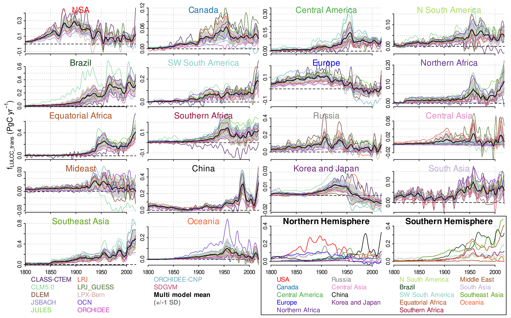
Figure A7 Region-wise smoothed annual f_{LULCC_trans} for different models from 1800 onward (compare Eq. 1). For a discussion of individual models refer to Sect. A1. The last two panels show regional ensemble means on a uniform scale.

Figure A8 Region-wise smoothed annual f_{LULCC_pi} for different models from 1800 onward (compare Eq. 2). For a discussion of individual models refer to Sect. A1. The last two panels show regional ensemble means on a uniform scale.

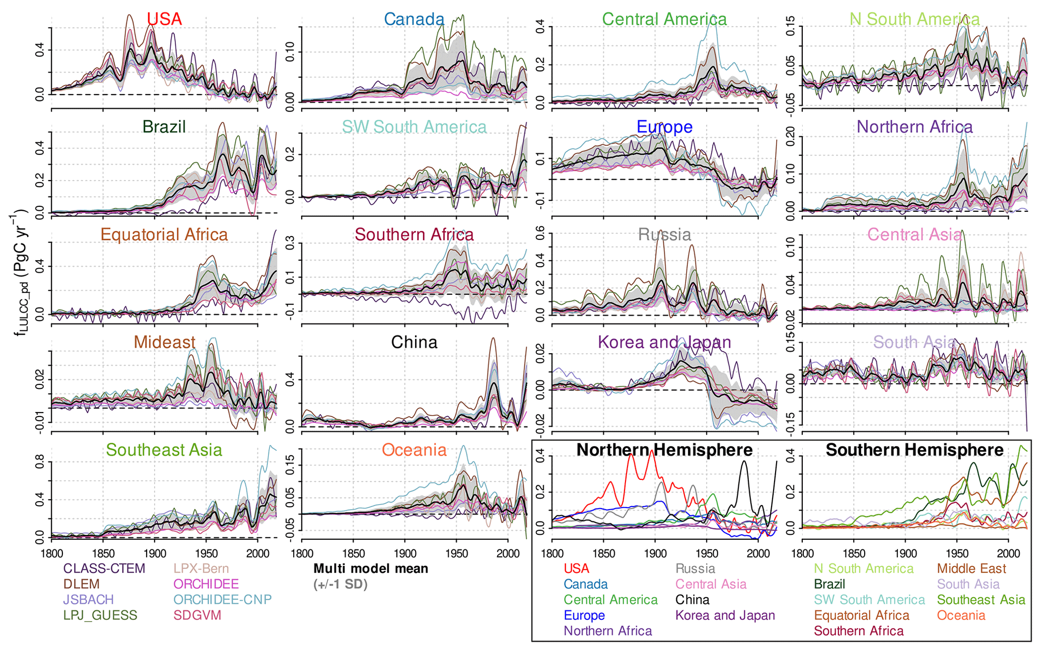
Figure A9 Region-wise smoothed annual f_{LULCC_pd} for different models from 1800 onward (compare Eq. 3). f_{LULCC_pd} was not derived for CLM5.0, JULES, LPJ, and OCN models (compare Table 2). For a discussion of individual models refer to Sect. A1. The last two panels show regional ensemble means on a uniform scale.

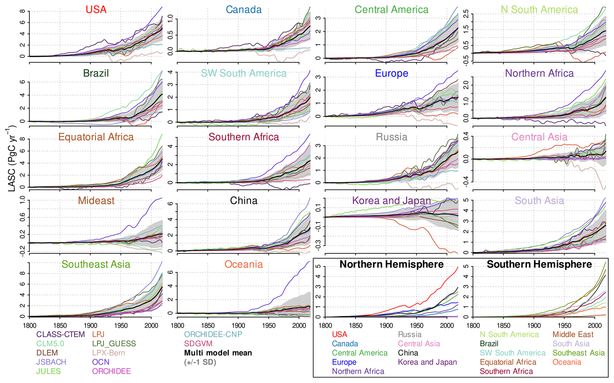
Figure A10 Region-wise smoothed cumulative loss of additional sink capacity (LASC) from 1800 onward (compare Eq. 4). For a discussion of individual models refer to Sect. A1. The last two panels show regional ensemble means on a uniform scale.

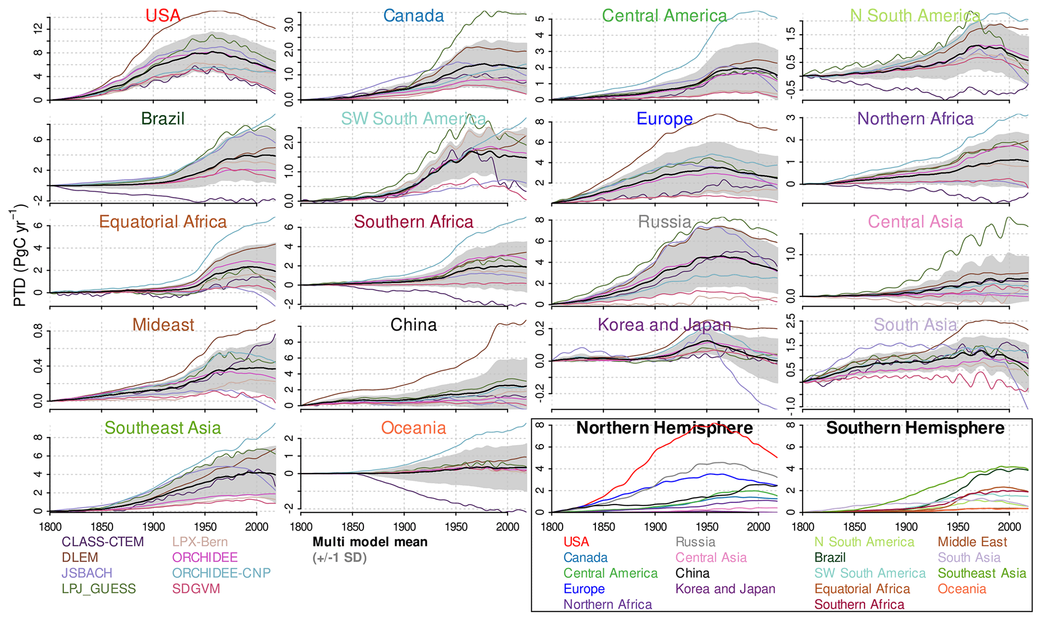
Figure A11 Region-wise smoothed cumulative “present-day” vs. “transient” environmental conditions difference in the f_LULCC (PTD) from 1800 onward (compare Eq. 5). The PTD was not derived for CLM5.0, JULS, LPJ, and OCN models (compare Table 2). For a discussion of individual models refer to Sect. A1. The last two panels show regional ensemble means on a uniform scale.

Figure A12 Region-wise smoothed cumulative difference between the f_LULCC under present-day and pre-industrial environmental conditions (environmental equilibrium difference, EED) from 1800 onward (compare Eq. 6). EED was not derived for CLM5.0, JULES, LPJ, and OCN models (compare Table 2). For a discussion of individual models refer to Sect. A1. The last two panels show regional ensemble means on a uniform scale.

Figure A13 Comparison of global annual NBP of the S0, S1, S2, and S3 simulation runs and derived f_{LULCC_trans} as aggregated in this study and published in the GCB2019 (Friedlingstein et al., 2019). The thick dashed lines (near or at 0) depict the differences (with respective colours). For the global values of this study, CDOs were used to convert NBP data per second to per year (multiplying seconds per day and, depending on the original temporal resolution, days per month or days per year) and to regrid data to the grid cell(multiplying with the area per grid cell). ORCHIDEE-CNP and SDGVM estimates were not shown since no data from the GCB2019 were available.

A1 Model variability in f_LULCC differences

The model spread in annual and cumulative f_LULCC estimates and their differences (LASC, PTD, and EED) has been shown to be large (compare Tables A1–A3) and increasing over time, in particular from 1950s onward in Brazil, northern Africa, equatorial Africa, and Southeast Asia (shaded areas in Figs. 3 and 4, showing the multi-model mean ±1 SD). This pronounced model spread can be explained by intertwining issues, such as the low quality of historical LULCC data (with different databases), the consideration or neglection of relevant processes (e.g. nitrogen fertilization), the simplified representation and uncertainty in the parameterization of management and natural processes, uncertainties in soil and vegetation C stocks, and the lack of observational constraints (Friedlingstein et al., 2019; Gasser et al., 2020; Lienert and Joos, 2018; Goll et al., 2015; Li et al., 2017).

The global EED and PTD were higher than in the other models for LPJ-GUESS, ORCHIDEE-CNP, and DLEM and lower for CLASS-CTEM, LPX-Bern and SDGVM. The PTD and EED show the highest model spread at the time of maximum LULCCs and towards the end of the simulation period, in particular in regions where vast areas of land were transformed (Brazil, equatorial Africa, Central, and South and Southeast Asia).

A particularly high model spread for global LASC at the end of the simulation period was found in Canada, north and southwest South America, Brazil, the Middle East, Korea, Japan, South and Southeast Asia, and Oceania with particularly high estimates for the OCN, CLASS-CTEM, LPJ-GUESS, and JSBACH models (Figs. A4 and A10).

High values in LPJ-GUESS likely result from high f_LULCC estimates with pronounced interannual variability (particularly prominent in Canada and Russia). This variability may be partially caused by stochastic components of the Globfirm fire model, which was used in the TRENDY LPJ-GUESS runs, causing fire emissions not necessarily synchronous in time between simulations runs.

High LASC estimates in JSBACH in Brazil and South and Southeast Asia can be explained by the strong positive response of forest productivity to rising CO₂ concentrations in the model and a consequently large LASC particularly upon clearing of tropical evergreen forests. High EED and PTD estimates in ORCHIDEE-CNP, in particular in Brazil, Southeast Asia, and equatorial and southern Africa, might result from accounting of phosphorus constraints on the biomass built up under elevated CO₂. ORCHIDEE-CNP simulates a more realistic sensitivity of plant productivity to elevated CO₂ than the version without nutrients, ORCHIDEE (discussed in detail in Sun et al., 2020), but more models are needed to draw robust conclusions about phosphorus effects on the f_LULCC.

LPX-Bern showed very low LASC, EED, and PTD estimates throughout the simulated period, which result from low f_LULCC estimates due to the exclusion of wood harvest and shifting cultivation and, particularly in most recent decades, due to the lack of tropical peatlands in the used configuration (for a detailed discussion refer to Lienert and Joos, 2018).

Low EED and PTD estimates in CLASS-CTEM likely result from a model change that led to different S0 simulations (control) for S1–S3 vs. S4–S6 simulations, which most probably also led to a pronounced variability and extreme values in some regional estimates.

JULES showed a remarkably high interannual variability for the LASC already in the early simulated period in particular in Canada, southwest South America, the Middle East, Korea, and Japan.

LPJ exhibited different interannual variability magnitudes for the pre-industrial and present-day land cover representation making it impossible to calculate the EED and PTD. The LPJ divergence in interannual variability may be due to differences in the carbon-climate sensitivity for managed grasslands and croplands compared to natural ecosystems and further work is needed to understand the mechanisms responsible.

Gasser et al. (2020)

Table A1 Overview of global annual f_LULCC estimates from this study: the ensemble of all 15 DGVMs and of two bookkeeping models (BLUE and H&N2017) from the annual global carbon budget (GCB2019; Friedlingstein et al., 2019), plus another recent bookkeeping estimate (Gasser et al., 2020). Emissions from peat fire and drainage were removed from the bookkeeping estimates to be better comparable to the DGVMs. Note that the error estimate of GCB2019's bookkeeping estimate of 0.7 PgC yr⁻¹ is an expert judgement, not direct model output. Minimum, maximum, and mean with standard deviation refer to the model ensemble.

Gasser et al. (2020)

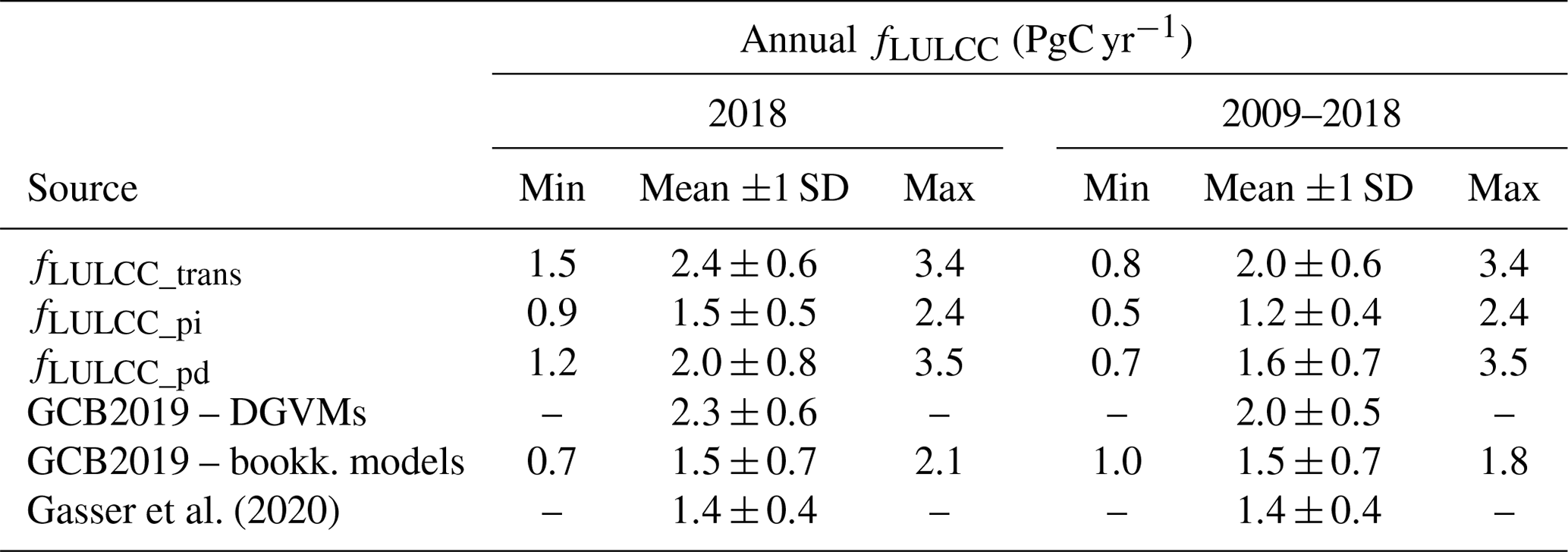
Table A2 Overview of global annual LASC estimates from this study (Friedlingstein et al. (2019) (GCB2019) and Gasser et al. (2020)). LASC estimates from GCB2019 and Gasser et al. (2020) are based on two different versions of OSCAR, which is constrained by DGVM estimates. Minimum, maximum, and mean with standard deviation refer to the model ensemble.

Gasser et al. (2020)Gasser et al. (2020)

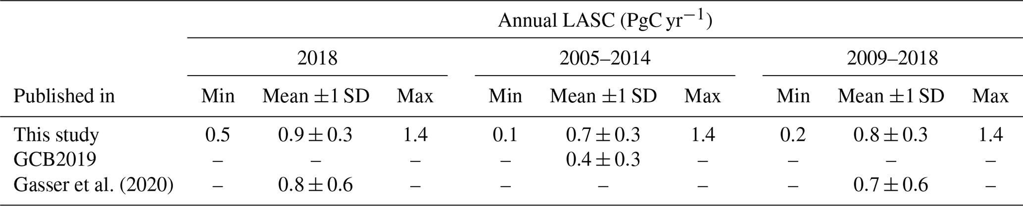
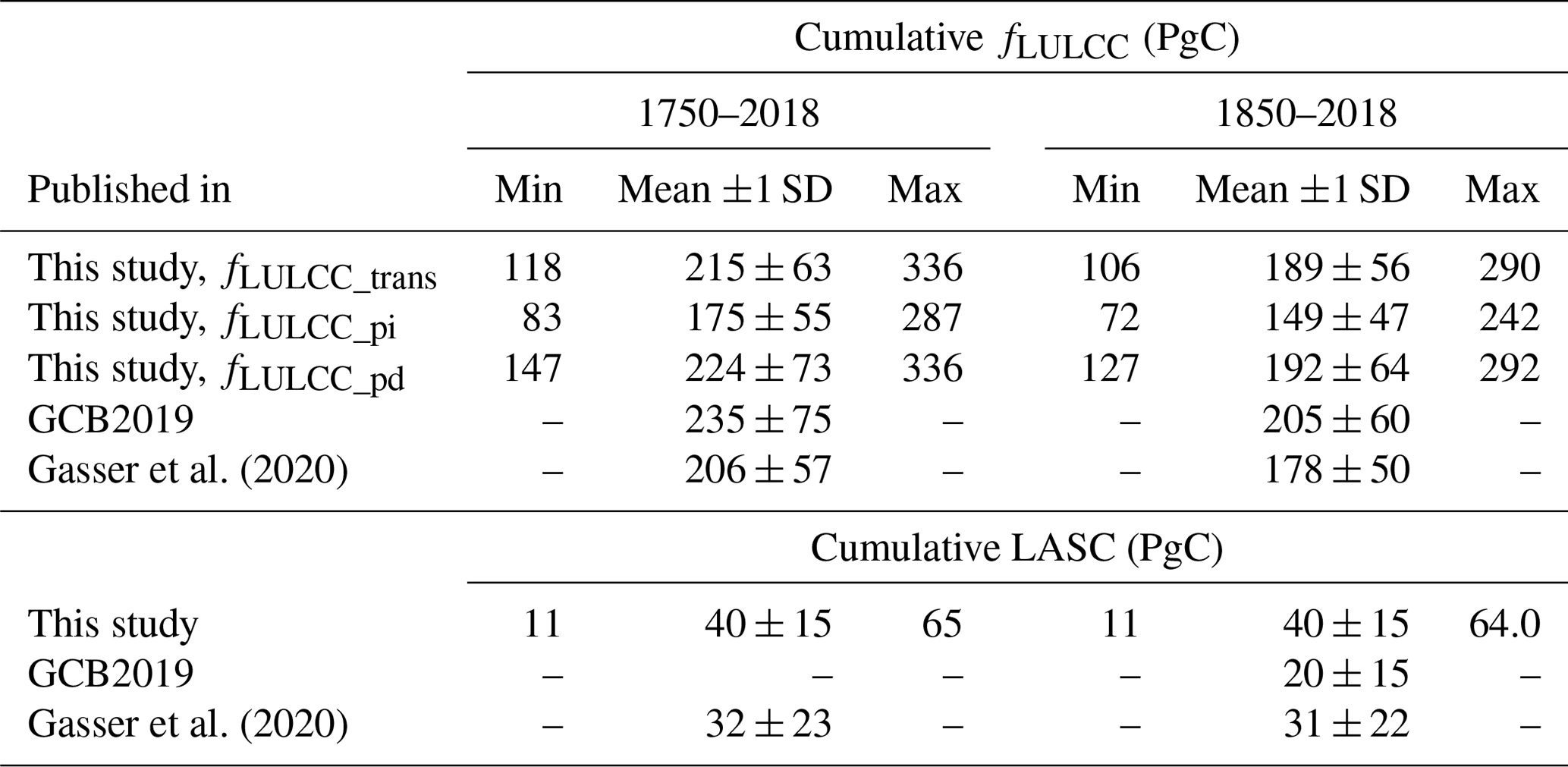
Table A3 Overview of global cumulative f_LULCC and LASC estimates from this study: the ensemble of 15 DGVMs and of two bookkeeping models (BLUE, Hansis et al., 2015 and Houghton and Nassikas, 2017) from the annual global carbon budget (GCB2019, Friedlingstein et al., 2019) plus another recent bookkeeping estimate (Gasser et al., 2020). Emissions from peat fire and drainage were removed from the bookkeeping estimates to be better comparable to the DGVMs. Note that mean cumulative GCB2019 estimates are based on bookkeeping models, while their uncertainty is derived from DGVMs. LASC estimates from GCB2019 and Gasser et al. (2020) are based on two different versions of OSCAR, which is constrained by DGVM estimates. Minimum, maximum, and mean with standard deviation refer to the model ensemble.