Regional variation in the effectiveness of methane-based and land-based climate mitigation options

Scenarios avoiding global warming greater than 1.5 or 2 ^∘C, as stipulated in the Paris Agreement, may require the combined mitigation of anthropogenic greenhouse gas emissions alongside enhancing negative emissions through approaches such as afforestation–reforestation (AR) and biomass energy with carbon capture and storage (BECCS). We use the JULES land surface model coupled to an inverted form of the IMOGEN climate emulator to investigate mitigation scenarios that achieve the 1.5 or 2 ^∘C warming targets of the Paris Agreement. Specifically, within this IMOGEN-JULES framework, we focus on and characterise the global and regional effectiveness of land-based (BECCS and/or AR) and anthropogenic methane (CH₄) emission mitigation, separately and in combination, on the anthropogenic fossil fuel carbon dioxide (CO₂) emission budgets (AFFEBs) to 2100. We use consistent data and socio-economic assumptions from the IMAGE integrated assessment model for the second Shared Socioeconomic Pathway (SSP2). The analysis includes the effects of the methane and carbon–climate feedbacks from wetlands and permafrost thaw, which we have shown previously to be significant constraints on the AFFEBs.

Globally, mitigation of anthropogenic CH₄ emissions has large impacts on the anthropogenic fossil fuel emission budgets, potentially offsetting (i.e. allowing extra) carbon dioxide emissions of 188–212 Gt C. This is because of (a) the reduction in the direct and indirect radiative forcing of methane in response to the lower emissions and hence atmospheric concentration of methane and (b) carbon-cycle changes leading to increased uptake by the land and ocean by CO₂-based fertilisation. Methane mitigation is beneficial everywhere, particularly for the major CH₄-emitting regions of India, the USA, and China. Land-based mitigation has the potential to offset 51–100 Gt C globally, the large range reflecting assumptions and uncertainties associated with BECCS. The ranges for CH₄ reduction and BECCS implementation are valid for both the 1.5 and 2 ^∘C warming targets. That is the mitigation potential of the CH₄ and of the land-based scenarios is similar for regardless of which of the final stabilised warming levels society aims for. Further, both the effectiveness and the preferred land management strategy (i.e. AR or BECCS) have strong regional dependencies. Additional analysis shows extensive BECCS could adversely affect water security for several regions. Although the primary requirement remains mitigation of fossil fuel emissions, our results highlight the potential for the mitigation of CH₄ emissions to make the Paris climate targets more achievable.

1 Introduction

The stated aims of the Paris Agreement of the United Nations Framework Convention on Climate Change (UNFCCC, 2015) are “to hold the increase in global average temperature to well below 2 ^∘C and to pursue efforts to limit the increase to 1.5 ^∘C”. The global average surface temperature for the decade 2006–2015 was 0.87 ^∘C above pre-industrial levels and is likely to reach 1.5 ^∘C between the years 2030 and 2052 if global warming continues at current rates (IPCC, 2018). The IPCC Special Report on Global Warming of 1.5 ^∘C (IPCC, 2018) gives the median remaining carbon budgets between 2018 and 2100 as 770 Gt CO₂ (210 Gt C) and 1690 Gt CO₂ (∼461 Gt C) to limit global warming to 1.5 ^∘C and 2 ^∘C, respectively. These budgets represent ∼20 and ∼41 years at present-day emission rates. The actual budgets could, however, be smaller, as they exclude Earth system feedbacks such as CO₂ released by permafrost thaw or CH₄ released by wetlands. Meeting the Paris Agreement goals will, therefore, require sustained reductions in sources of fossil carbon emissions, other long-lived anthropogenic greenhouse gases (GHGs), and some short-lived climate forcers (SLCFs) such as methane (CH₄), alongside increasingly extensive implementations of carbon dioxide removal (CDR) technologies (IPCC, 2018). Accurate information is needed about the range and efficacy of options available to achieve this.

Biomass energy with carbon capture and storage (BECCS) and afforestation–reforestation (AR) are among the most widely considered CDR technologies in the climate and energy literature (Minx et al., 2018). For scenarios consistent with a 2 ^∘C warming target, the review by Smith et al. (2016) finds this may require (i) a median removal of 3.3 Gt C yr⁻¹ from the atmosphere through BECCS by 2100 and (ii) a mean CDR through AR of 1.1 Gt C yr⁻¹ by 2100, giving a total CDR equivalent to 47 % of present-day emissions from fossil fuel and other industrial sources (Le Quéré et al., 2018). Although there are fewer scenarios that look specifically at the 1.5 ^∘C pathway, BECCS is still the major CDR approach (Rogelj et al., 2018). For the default assumptions in Fuss et al. (2018), BECCS would remove a median of 4 Gt C by 2100 and a total of 41–327 Gt C from the atmosphere during the 21st century, equivalent to about 4–30 years of current annual emissions. The land requirements for BECCS will be greater for the 1.5 ^∘C target within a given shared socio-economic pathway (e.g. SSP2), although published estimates are similar for the two warming targets, with between 380–700 Mha required for the 2 ^∘C target (Smith et al., 2016) and greater than 600 Mha for the 1.5 ^∘C target (van Vuuren et al., 2018). This is because the land requirements for bioenergy production differ strongly across the different SSPs, depending on assumptions about the contribution of residues, assumed yields and yield improvements, start dates of implementation, and the rates of deployment. While the CDR figures assume optimism about the mitigation potential of BECCS, concerns have been raised about the potentially detrimental impacts of BECCS on food production, water availability and biodiversity (e.g. Heck et al., 2018; Krause et al., 2017). Others note the risks and query the feasibility of large-scale deployment of BECCS (e.g. Anderson and Peters, 2016; Vaughan and Gough, 2016; Vaughan et al., 2018).

Harper et al. (2018) find the overall effectiveness of BECCS to be strongly dependent on the assumptions concerning yields, the use of initial above-ground biomass that is replaced, and the calculated fossil fuel emissions that are offset in the energy system. Notably, if BECCS involves replacing ecosystems that have higher carbon contents than energy crops, then AR and avoided deforestation can be more efficient than BECCS for atmospheric CO₂ removal over this century (Harper et al., 2018).

Mitigation of the anthropogenic emissions of non-CO₂ GHGs such as CH₄ and of SLCFs such as black carbon have been shown to be attractive strategies with the potential to reduce projected global mean warming by 0.22–0.5 ^∘C by 2050 (Shindell et al., 2012; Stohl et al., 2015). It should be noted that these were based on scenarios with continued use of fossil fuels. Through the link to tropospheric ozone (O₃), there are additional co-benefits of CH₄ mitigation for air quality, plant productivity and food production (Shindell et al., 2012), and carbon sequestration (Oliver et al., 2018). Control of anthropogenic CH₄ emissions leads to rapid decreases in its atmospheric concentration, with an approximately 9-year removal lifetime (and as such is an SLCF). Furthermore, many CH₄ mitigation options are inexpensive or even cost-negative through the co-benefits achieved (Stohl et al., 2015), although expenditure becomes substantial at high levels of mitigation (Gernaat et al., 2015). The extra “allowable” carbon emissions from CH₄ mitigation can make a substantial difference to the feasibility or otherwise of achieving the Paris climate targets (Collins et al., 2018).

Some increases in atmospheric CH₄ are not related to direct anthropogenic activity but indirectly to climate change triggering natural carbon and methane–climate feedbacks. These effects could act as positive feedbacks and thus in the opposite direction to the mitigation of anthropogenic CH₄ sources. Wetlands are the largest natural source of CH₄ to the atmosphere and these emissions respond strongly to climate change (Gedney et al., 2019; Melton et al., 2013). A second natural feedback is from permafrost thaw. In a warming climate, the resulting microbial decomposition of previously frozen organic carbon is potentially one of the largest feedbacks from terrestrial ecosystems (Schuur et al., 2015). As the carbon and CH₄ climate feedbacks from natural wetlands and permafrost thaw could be substantial, this causes a reduction in anthropogenic CO₂ emission budgets compatible with climate change targets (Comyn-Platt et al., 2018a; Gasser et al., 2018).

This paper models the potential for mitigation of greenhouse gases to contribute to meeting the Paris targets of limiting global warming to 1.5 ^∘C and 2 ^∘C, respectively. Specifically, we investigate the effectiveness of mitigation of anthropogenic methane emissions and land-based mitigation (e.g. implementation of BECCS and AR), combining results from three recent papers (Collins et al., 2018; Comyn-Platt et al., 2018a; Harper et al., 2018). We determine the effectiveness of these approaches in terms of their impact on the anthropogenic fossil fuel CO₂ emissions budget consistent with stabilising temperature at 1.5 and 2 ^∘C of warming. The more effective the mitigation option, the larger the fossil fuel CO₂ emissions budget can be consistent with stabilisation at a given level. We estimate the impact of these mitigation scenarios relative to an existing scenario of greenhouse gas concentrations (based on the IMAGE SSP2 baseline), spanning uncertainties in both climate model projections (both global warming and regional climate change), process representation, and the efficacy of BECCS. Section 2 provides a brief description of the models, the experimental set-up, and the key datasets used in the model runs and subsequent analysis. Section 3 presents and discusses the results, starting with a global perspective before addressing the regional dimension. For BECCS, we additionally investigate the sensitivity to key assumptions and consider the implications for water security. Section 4 contains our conclusions.

2 Approach and methodology

Our overall modelling strategy is as follows. The starting point is the prescription of global temperature profiles that match the historical record, followed by a transition to a future stabilisation at either 1.5 or 2.0 ^∘C above pre-industrial levels. For these profiles, we then determine the related pathways in atmospheric radiative forcing by inversion of the global energy balance component of the IMOGEN impacts model. IMOGEN “Integrated Model Of Global Effects of climatic aNomalies” (Sect. 2.2) (Comyn-Platt et al., 2018a; Huntingford et al., 2010) is an intermediate complexity climate model, which emulates 34 models in the CMIP5 climate model ensemble. Hence, our radiative forcing (RF) trajectories have uncertainty bounds, reflecting the different climate sensitivities of existing climate models.

For each radiative forcing pathway, we subtract the individual RF components for non-CO₂ and non-CH₄ radiatively active gases that are perturbed by human activity, using baseline and mitigation scenarios taken from the IMAGE integrated assessment model. Following this, for CH₄ we represent its atmospheric chemistry by a single atmospheric lifetime to translate the methane emissions into atmospheric concentrations. The related RF for CH₄ is also subtracted from the overall value. Hence, the remaining RF is that available for changes to atmospheric CO₂ concentration. The IMOGEN model uses pattern scaling, again fitted to the same 34 climate models, to estimate local changes in near-surface meteorology. Combined with our global temperature pathways, these pattern-based changes (as well as atmospheric CO₂ concentration) drive the Joint UK Land-Environment Simulator land surface model (JULES, Sect. 2.1) (Best et al., 2011; Clark et al., 2011). JULES estimates atmosphere–land CO₂ exchange, and IMOGEN similarly contains a single global description of oceanic CO₂ draw-down. These two estimates of carbon exchanges with the land and ocean, respectively, in conjunction with atmospheric storage being linear in the CO₂ pathway, finally determine by simple summation compatible CO₂ emissions from fossil fuel burning. We call this the anthropogenic (CO₂) fossil fuel emission budgets (AFFEB) compatible with the warming pathway, subject to the assumptions made for non-CO₂ forcings.

Our numerical simulation structure allows us to investigate the implications of three different key changes on AFFEB for stabilisation at both 1.5 and 2.0 ^∘C and in a structure that captures features of a full set of climate models. First and maybe most importantly, we work to understand how regional reductions in CH₄ emissions allow higher values of AFFEB. Second, we consider how alternative scenarios of BECCS implementation alter atmosphere–land CO₂ exchanges and again present the resultant implications for AFFEB. Third, we determine how the newer understanding of warming impacts on wetland methane emissions also affects AFFEB. Figure 1 captures the modelling framework, derivation of AFFEB, and our numerical experiments in a single overall schematic diagram.

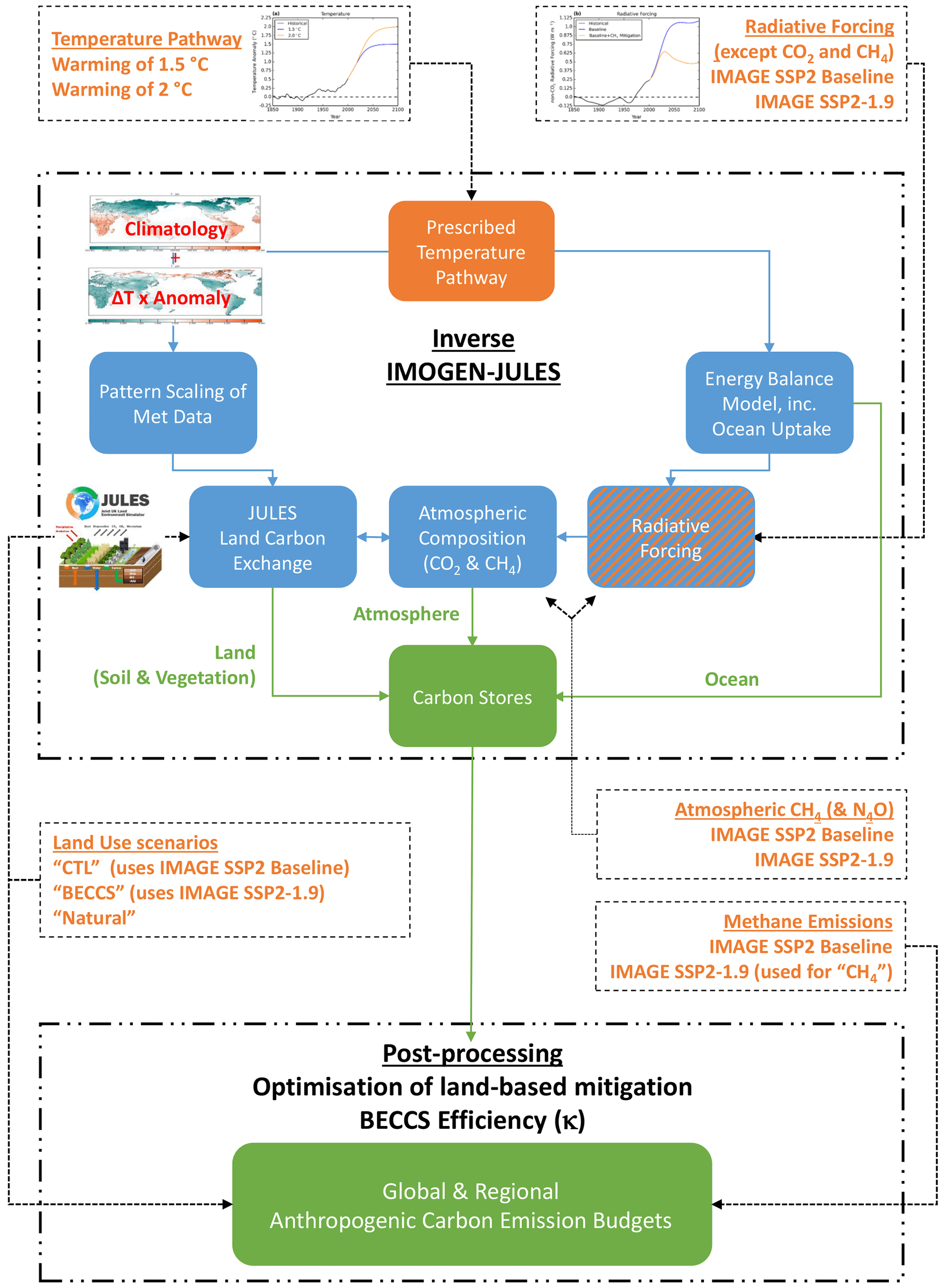
Figure 1 Schematic of the modelling approach and the workflow. The coloured boxes and text show the key components of the inverted IMOGEN-JULES model (blue), the prescribed and input data used in this study (orange), and the outputs (green).

Each of the scenarios investigated using the IMOGEN-JULES framework comprises 2 ensembles of 136 members, one ensemble for each of the warming targets. We make use of these ensembles to derive an “uncertainty” in the derived carbon budgets, specifically from climate change (as given by the 34 CMIP5 models) and from key land surface processes (methane emissions from wetlands and the ozone vegetation damage). The climate change uncertainty comprises both the range of climate sensitivities of the CMIP5 models and the different regional patterns in the models. We use the median of the 136-member ensemble as the central value to derive the carbon budgets and the interquartile range (25 %–75 %) for the uncertainty.

2.1 The JULES model

We use the JULES land surface model (Best et al., 2011; Clark et al., 2011), release version 4.8 but with a number of additions required specifically for our analysis.

1. Land use. We adopt the approach used by Harper et al. (2018) and prescribe managed land use and land use change (LULUC). On land used for agriculture, C₃ and C₄ grasses are allowed to grow to represent crops and pasture. The land use mask consists of an annual fraction of agricultural land in each grid cell. Historical LULUC is based on the HYDE 3.1 dataset (Klein Goldewijk et al., 2011), and future LULUC is based on two scenarios (SSP2 RCP1.9 and SSP2 baseline), which were developed for use in the IMAGE integrated assessment model (IAM) (Doelman et al., 2018; van Vuuren et al., 2017) (see also Sect. 2.3).

   Natural vegetation is represented by nine plant functional types (PFTs): broadleaf deciduous trees, tropical broadleaf evergreen trees, temperate broadleaf evergreen trees, needle-leaf deciduous trees, needle-leaf evergreen trees, C₃ and C₄ grasses, and deciduous and evergreen shrubs (Harper et al., 2016). These PFTs are in competition for space in the non-agricultural fraction of grid cells, based on the TRIFFID (Top-down Representation of Interactive Foliage and Flora Including Dynamics) dynamic vegetation module within JULES (Clark et al., 2011). A further four PFTs are used to represent agriculture (C₃ and C₄ crops and C₃ and C₄ pasture), and harvest is calculated separately for food and bioenergy crops (see Sect. 2.4.3, where we describe the modelling of carbon removed via bioenergy with CCS). When natural vegetation is converted to managed agricultural land, the vegetation carbon removed is placed into woody product pools that decay at various rates back into the atmosphere (Jones et al., 2011). Hence, the carbon flux from LULUC is not lost from the system. There are also four non-vegetated surface types: urban, water, bare soil, and ice.

2. Soil carbon. Following Comyn-Platt et al. (2018a), we also use a 14-layered soil column for both hydro-thermal (Chadburn et al., 2015) and carbon dynamics (Burke et al., 2017b). Burke et al. (2017a) demonstrated that modelling the soil carbon fluxes as a multi-layered scheme improves estimates of soil carbon stocks and net ecosystem exchange. In addition to the vertically discretised respiration and litter input terms, the soil–carbon balance calculation also includes a diffusivity term to represent cryoturbation–bioturbation processes. The freeze–thaw process of cryoturbation is particularly important in cold permafrost-type soils (Burke et al., 2017a). Following Burke et al. (2017b), we diagnose permafrost wherever the deepest soil layer is below 0 ^∘C (assuming that this layer is below the depth of zero annual amplitude, i.e. where seasonal changes in ground temperature are negligible (≤0.1 ^∘C)). Further, for permafrost regions, there is an additional variable to trace or diagnose “old” carbon and its release from permafrost as it thaws.

   The multi-layered methanogenesis scheme improves the representation of high latitude CH₄ emissions, where previous studies underestimated production at cold permafrost sites during “shoulder seasons” (Zona et al., 2016). Figure 2 shows the annual cycle in the observed and modelled wetland CH₄ emissions at the Samoylov Island field site (Fig. 2a) and a comparison of observed and modelled annual mean fluxes at this and other sites (Fig. 2b). The range of uncertainty used in our study (JULES low Q₁₀–JULES high Q₁₀) captures the range of uncertainty in the observations. In Fig. 2b, the error bars denote the lower and upper estimates from the low and high Q₁₀ simulations. The symbols represent the mean value between these estimates. Further, the layered methane scheme used in this work gives a better description of the shoulder season emissions when compared with the original, non-layered methane scheme in JULES. The multi-layered scheme allows an insulated sub-surface layer of active methanogenesis to continue after the surface has frozen. These model developments not only improve the seasonality of the emissions but more importantly for this study capture the release of carbon as CH₄ from deep soil layers, including thawed permafrost. Further evaluation of the multi-layer scheme can be found in Chadburn et al. (2020).

3. Methane from wetlands. Following Comyn-Platt et al. (2018a), we also use the multi-layered soil carbon scheme described in (2) above to give the local land–atmosphere CH₄ flux, $E_{{\mathrm{CH}}_{\mathrm{4}}}$ (kg C m⁻² s⁻¹):

   $$\begin{array}{}\text{(1)}& \begin{array}{rl}{E}_{{\mathrm{CH}}_{\mathrm{4}}}& =k\cdot f_{\mathrm{wetl}}\cdot \sum _{i=\mathrm{1}}^{n{C}_{\mathrm{s}}\mathrm{pools}}{\mathit{\kappa }}_i\cdot \sum _{z=\mathrm{0}\mathrm{m}}^{z=\mathrm{3}\mathrm{m}}{e}^{-\mathit{\gamma }z}{C}_{{\mathrm{s}}_{i,z}}\\ & \cdot Q_{\mathrm{10}}{\left(T_{{\mathrm{soil}}_z}\right)}^{\mathrm{0.1}\left(T_{{\mathrm{soil}}_z}-T_{\mathrm{0}}\right)},\end{array}\end{array}$$

   where k is a dimensionless scaling constant such that the global annual wetland CH₄ emissions are 180 Tg CH₄ in 2000 (as described in Comyn-Platt et al., 2018a), z is the depth in soil column (in m), i is the soil carbon pool, f_wetl (–) is the fraction of wetland area in the grid cell, κ_i (s⁻¹) is the specific respiration rate of each pool (Table 8 of Clark et al., 2011), C_s (kg m⁻²) is soil carbon, and T_soil (K) is the soil temperature. The decay constant γ (=0.4 m⁻¹) describes the reduced contribution of CH₄ emission at deeper soil layers due to inhibited transport and increased oxidation through overlaying soil layers. This representation of inhibition and of the pathways for CH₄ release to the atmosphere (e.g. by diffusion, ebullition, and vascular transport) is a simplification. However, previous work that explicitly represented these processes showed little to no improvement when compared with in situ observations (McNorton et al., 2016). We do not model CH₄ emissions from freshwater lakes (and oceans).

   Comyn-Platt et al. (2018a) varied Q₁₀ in Eq. (1) to encapsulate a range of methanogenesis process uncertainty. They derive Q₁₀ values for each GCM configuration to represent two wetland types identified in Turetsky et al. (2014) (“poor-fen” and “rich-fen”). They also include a third “low-Q₁₀”, which gives increased importance to high-latitude emissions. Their ensemble spread was able to describe the magnitude and distribution of present-day CH₄ emissions from natural wetlands, according to the models used in the then-current global methane assessment (Saunois et al., 2016). Here, we use the “low-Q₁₀” value of Comyn-Platt et al. (2018a) (=2.0) and adopt a “high-Q₁₀” value of ∼4.8 from the rich-fen parameterisation. The two Q₁₀ values used here still capture the full range of the methanogenesis process uncertainty.

4. Ozone vegetation damage. We use a JULES configuration including ozone deposition damage to plant stomata, which affects land–atmosphere CO₂ exchange (Sitch et al., 2007). JULES requires surface atmospheric ozone concentrations, O₃ (ppb), for the duration of the simulation period (1850–2100). As in Collins et al. (2018), we do not model tropospheric ozone production from CH₄ explicitly in IMOGEN. Instead, we use two sets of monthly near-surface O₃ concentration fields (January–December) from HADGEM3-A GA4.0 model runs, with the sets corresponding to low (1285 ppbv) and high (2062 ppbv) global mean atmospheric CH₄ concentrations (Stohl et al., 2015). We assume that the atmospheric O₃ concentration in each grid cell responds linearly to the atmospheric CH₄ concentration. We derive separate linear relationships for each month and grid cell and use these to calculate the surface O₃ concentration from the corresponding global atmospheric CH₄ concentration as it evolves during the IMOGEN run (Sect. 2.2.1). We use CH₄ concentration profiles from the IMAGE SSP2 Baseline and RCP1.9 scenarios (Sect. 2.3.1) adjusted for natural methane sources (see 3 above and Sect. 2.3.3). We undertake runs using both the “high” and “low” vegetation ozone damage parameter sets (Sitch et al., 2007).

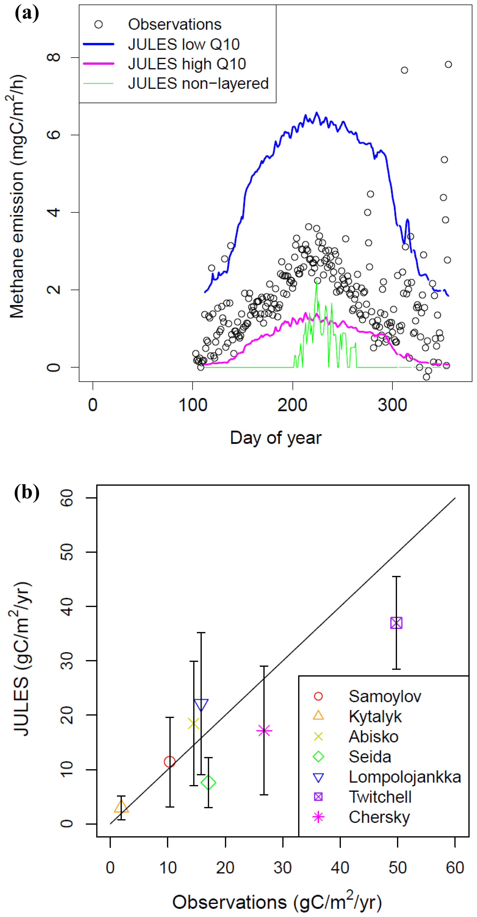
Figure 2 (a) Observed (circles) and modelled wetland methane emissions at the Samoylov Island field site. Modelled wetland methane emissions are shown for the standard JULES non-layered soil carbon configuration (green) and for the JULES layered soil carbon configurations with low (blue line) and high (magenta line) Q₁₀ temperature sensitivities; the low Q₁₀ configuration gives higher methane emissions at high-latitude sites such as the Samoylov Island field site. The methane emission data are preliminary and were provided by Lars Kutzbach and David Holl. (b) Comparison of observed and modelled annual mean wetland CH₄ emission fluxes at a number of northern high-latitude and temperate sites. The error bars denote the lower and upper estimates from the low and high Q₁₀ simulations. The symbols represent the mean value between these estimates.

2.2 The IMOGEN intermediate complexity climate model

2.2.1 IMOGEN

The IMOGEN climate impacts model (Huntingford et al., 2010) uses “pattern-scaling” to estimate changes to the seven meteorological variables required to drive JULES. Huntingford et al. (2010) assume that changes in local temperature, precipitation, humidity, wind speed, surface short-wave and long-wave radiation, and pressure are linear in global warming. Spatial patterns of each variable (based on the 34 GCM simulations in CMIP5, Comyn-Platt et al., 2018a) are multiplied by the amount of global warming over land, ΔT_L, to give local monthly predictions of climate change. When using IMOGEN in forward mode, ΔT_L is calculated with an energy balance model (EBM) as a function of the overall changes in radiative forcing, ΔQ (W m⁻²). ΔQ is the sum of the atmospheric greenhouse gas contributions (Eq. 2) (Etminan et al., 2016), which in the forward mode are either calculated (CO₂ and CH₄) or prescribed (for other atmospheric contributors) on a yearly time step.

$$\begin{array}{}\text{(2)}& \begin{array}{rl}\mathrm{\Delta }Q\left(\mathrm{total}\right)& =\mathrm{\Delta }Q\left({\mathrm{CO}}_{\mathrm{2}}\right)+\mathrm{\Delta }Q\left(\mathrm{non}{\mathrm{CO}}_{\mathrm{2}}\mathrm{GHGs}\right)\\ & +\mathrm{\Delta }Q\left(\mathrm{aerosols}\mathrm{and}\mathrm{other}\mathrm{climate}\mathrm{forcers}\right)\end{array}\end{array}$$

The EBM includes a simple representation of the ocean uptake of heat and CO₂ and uses a separate set of four parameters for each climate and Earth system model emulated (Huntingford et al., 2010): the climate feedback parameters over land and ocean, λ_l and λ_o (W m⁻² K⁻¹), respectively, the oceanic “effective thermal diffusivity”, κ (W m⁻¹ K⁻¹), representing the ocean thermal inertia and a land–sea temperature contrast parameter, ν, linearly relating warming over land, ΔT_l (K), to warming over ocean, ΔT_o (K), as ΔT_l=νΔT_o. The climate feedback parameters (λ_l and λ_o) are calibrated using model-specific data for the top of the atmosphere radiative fluxes, the mean land and ocean surface temperatures, and an estimate of the radiative forcing modelled for the CO₂ changes.

The atmospheric CH₄ concentrations available from the IMAGE database (see Sect. 2.3.1) assume a constant annual wetland CH₄ emission (van Vuuren et al., 2017). However, these emissions have interannual variability and a positive climate feedback (Comyn-Platt et al., 2018a; Gedney et al., 2019), and their correct representation is a central part of our study. We follow the same approach that we used in our previous studies (Collins et al., 2018; Comyn-Platt et al., 2018a; Gedney et al., 2019). As the IMOGEN-JULES modelling framework does not have an explicit representation of the atmospheric chemistry of methane, we represent the oxidation and hence loss of CH₄ by a single lifetime (τ).

$$\begin{array}{}\text{(3)}& \begin{array}{rl}{\displaystyle \frac{\mathrm{d}\left(\left[{\mathrm{CH}}_{\mathrm{4}}\right]-{\left[{\mathrm{CH}}_{\mathrm{4}}\right]}_{\mathrm{IMAGE}}\right)}{\mathrm{d}t}}& =C\left\{\sum F\left[{\mathrm{CH}}_{\mathrm{4}}\right]\right.\\ & \left.-\sum F{\left[{\mathrm{CH}}_{\mathrm{4}}\right]}_{\mathrm{IMAGE}}\right\}\\ & -{\displaystyle \frac{\left[{\mathrm{CH}}_{\mathrm{4}}\right]-{\left[{\mathrm{CH}}_{\mathrm{4}}\right]}_{\mathrm{REF}}}{\mathit{\tau }}}\end{array}\end{array}$$

Here, [CH₄] and [CH₄]_IMAGE are the atmospheric methane concentrations using our new wetland-based, time-varying (F[CH₄]) and the constant IMAGE (F[CH₄]_IMAGE) wetland emissions, respectively. Parameter C is a constant to convert from Tg CH₄ to a mixing ratio in parts per billion by volume (ppbv). Further, higher atmospheric concentrations of CH₄ and its oxidation product (carbon monoxide) lower the concentration of hydroxyl radicals, the major removal reaction for CH₄, thereby increasing the atmospheric lifetime of CH₄. Conversely, lower CH₄ concentrations will shorten its atmospheric lifetime. We take account of this feedback of CH₄ on its lifetime (τ) using Eq. (4) (Collins et al., 2018; Comyn-Platt et al., 2018a; Gedney et al., 2019),

$$\begin{array}{}\text{(4)}& \begin{array}{rl}\ln \left(\mathit{\tau }/{\mathit{\tau }}_{\mathrm{o}}\right)=& s\cdot \ln \left(\left[{\mathrm{CH}}_{\mathrm{4}}\right]/{\left[{\mathrm{CH}}_{\mathrm{4}}\right]}_{\mathrm{o}}\right),\\ & \mathrm{i}.\mathrm{e}.,\mathit{\tau }={\mathit{\tau }}_{\mathrm{o}}\exp \left(s\left[{\mathrm{CH}}_{\mathrm{4}}\right]/{\left[{\mathrm{CH}}_{\mathrm{4}}\right]}_{\mathrm{o}}\right).\end{array}\end{array}$$

In Eq. (4), [CH₄]_o and τ_o are the contemporary atmospheric CH₄ concentration and lifetime, and s is the CH₄–OH feedback factor, defined by $s=\partial \ln \left(\mathit{\tau }\right)/\partial \ln \left({\mathrm{CH}}_{\mathrm{4}}\right)$. We take values of τ_o=8.4 years, [CH₄]_o=1745 ppbv, and s=0.28 from Ehhalt et al. (2001, p. 248 and 250). In our earlier study on the climate–wetland methane feedback (Gedney et al., 2019), we investigated the sensitivity to the methane lifetime and the feedback factor, in addition to an analysis of the main drivers on the wetland methane–climate feedback and the main sources of uncertainty. Gedney et al. (2019) conclude that the limited knowledge of contemporary global wetland emissions is a larger source of uncertainty than that from the projected climate spread of the 34 GCMs. We quantify this uncertainty in our experimental design by using two values of Q₁₀ (see Sect. 2.1).

In response to our dynamic interactive calculations of atmospheric CH₄ concentrations, we derive the related change in methane radiative forcing (RF). We use the formulation from Etminan et al. (2016), which accounts for the short-wave absorption by CH₄ and the overlap with N₂O. The atmospheric oxidation of methane (by the hydroxyl radical) leads to the production of tropospheric ozone and stratospheric water vapour. We calculate these indirect contributions of methane to the overall radiative forcing, following the approach for methane adopted in our previous work (Collins et al., 2018; Comyn-Platt et al., 2018a; Gedney et al., 2019). Collins et al. (2018) represent the forcing contributions from O₃ and stratospheric water vapour as linear functions of the CH₄ mixing ratio, based on the analysis presented in IPCC AR5 (Myhre et al., 2013). The indirect methane forcings amount to $\mathrm{2.36}\times {\mathrm{10}}^{-\mathrm{4}}\pm \mathrm{1.09}\times {\mathrm{10}}^{-\mathrm{4}}$ W m⁻² per ppb CH₄ (i.e. 0.65±0.3 times the CH₄ radiative efficiency). Hence, we incorporate the indirect effects of these CH₄ emission changes by an approximation, multiplying the CH₄ radiative forcing by 1.65.

In this study, we use the inverse version of IMOGEN, which follows prescribed temperature pathways (Fig. 3a), to derive the total radiative forcing (ΔQ[total]) and then the CO₂ radiative forcing (ΔQ[CO₂]), using Eq. (2). Comyn-Platt et al. (2018a) describe the changes made to the EBM to create the inverse version. As each of the 34 GCMs that IMOGEN emulates has a different set of EBM parameters, each GCM has a different time-evolving radiative forcing (ΔQ) estimate for a given temperature pathway, ΔT_G(t). When IMOGEN is forced with a historical record of ΔT_G, the range of ΔQ for the near present-day values (year 2015) from the 34 GCMs is 1.13 W m⁻². To ensure a smooth transition to the modelled future, we require the historical period, 1850–2015, to match observations of both ΔT_G and atmospheric composition for all GCMs. As we have a model-specific estimate of the radiative forcing modelled for the CO₂ changes (see above), we therefore attribute the spread in ΔQ to the uncertainty in the non-CO₂ radiative forcing component, particularly the atmospheric aerosol contribution, which has an uncertainty range of −0.5 to −4 W m⁻² (Stocker et al., 2013). Apart from our modelled CH₄ and CO₂ radiative forcings and the potential future balances between them, we use the projections from the IMAGE SSP2 baseline or RCP1.9 scenario for the radiative forcing of other atmospheric contributors (Fig. 3b).

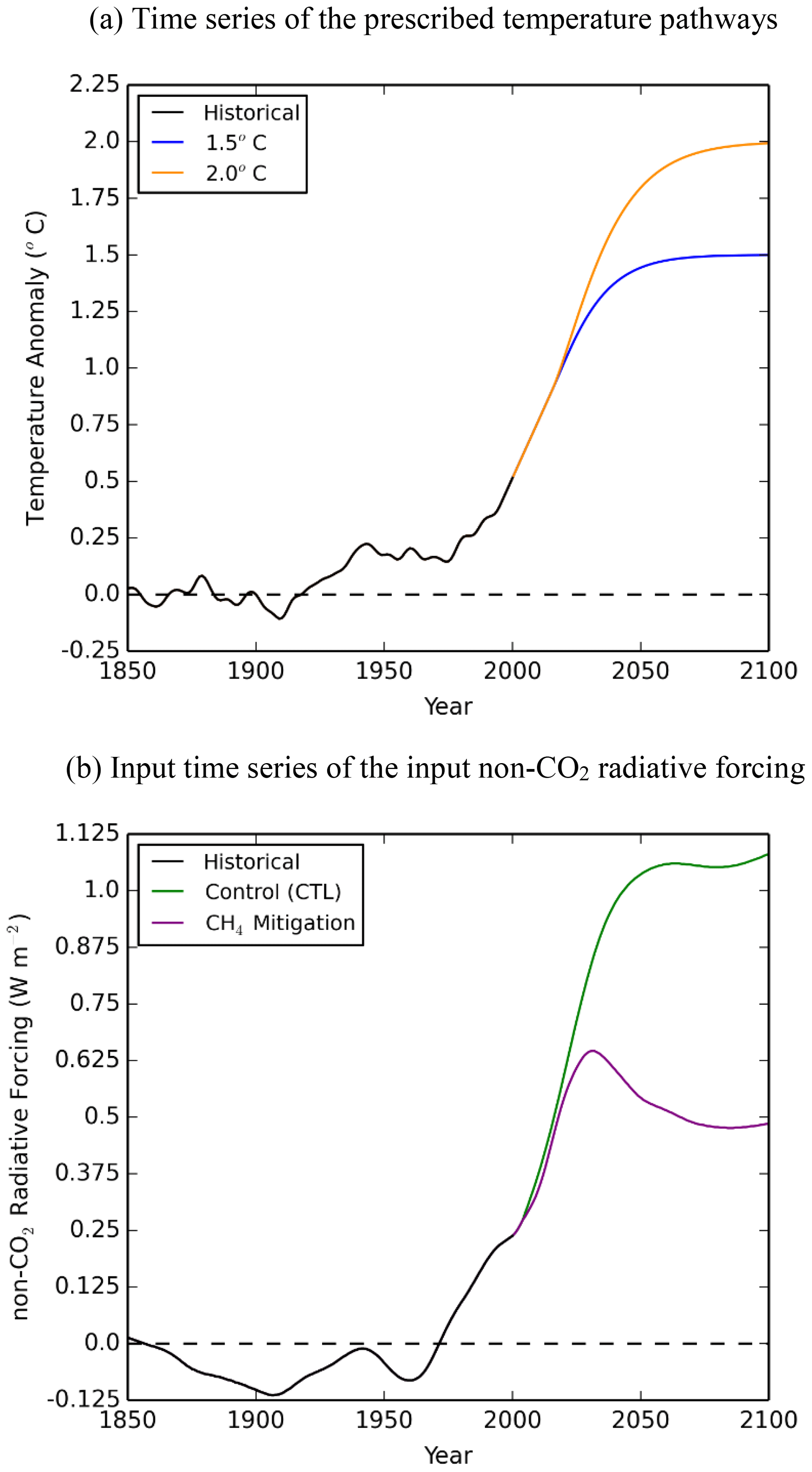
Figure 3 Time series of key datasets used in the study. (a) The historic temperature record (black) and the prescribed temperature profiles used to represent warming of 1.5 ^∘C (blue) and 2 ^∘C (orange). (b) The historic (black) and the projected non-CO₂ greenhouse gas radiative forcing (W m⁻²) for the control (green) and methane mitigation (purple) scenarios.

2.2.2 Temperature profile formulation

Huntingford et al. (2017) define a framework to create trajectories of global temperature increase, based on two parameters, and which model the efforts of humanity to limit emissions of greenhouse gases and short-lived climate forcers, and, if necessary, capture atmospheric carbon. These profiles have the mathematical form of

$$\begin{array}{}\text{(5)}& \mathrm{\Delta }T\left(t\right)=\mathrm{\Delta }{T}_{\mathrm{0}}+\mathit{\gamma }t-\left(\mathrm{1}-e^{-\mathit{\mu }\left(t\right)t}\right)\left[\mathit{\gamma }t-\left(\mathrm{\Delta }{T}_{\mathrm{Lim}}-\mathrm{\Delta }{T}_{\mathrm{0}}\right)\right],\end{array}$$

where ΔT(t) is the change in temperature from pre-industrial levels at year t, ΔT₀ is the temperature change at a given initial point (in this case ΔT₀=0.89 ^∘C for 2015), ΔT_Lim is the final prescribed warming limit, and

$$\begin{array}{}\text{(6)}& \mathit{\mu }\left(t\right)={\mathit{\mu }}_{\mathrm{0}}+{\mathit{\mu }}_{\mathrm{1}}t\mathrm{and}\mathit{\gamma }=\mathit{\beta }-{\mathit{\mu }}_{\mathrm{0}}\left(\mathrm{\Delta }{T}_{\mathrm{Lim}}-\mathrm{\Delta }{T}_{\mathrm{0}}\right),\end{array}$$

where β (= 0.00128) is the current rate of warming and μ₀ and μ₁ are tuning parameters that describe anthropogenic attempts to stabilise global temperatures (Huntingford et al., 2017). The parameter values used for the two profiles are as follows: (a) the 1.5 ^∘C profile uses ΔT_lim=1.5 ^∘C, μ₀=0.1, and μ₁=0.0, and (b) the 2 ^∘C profile uses ΔT_lim=2 ^∘C, μ₀=0.08, and μ₁=0.0.

2.3 Scenarios and model runs

We undertake a control run and other simulations with anthropogenic CH₄ mitigation or land-based mitigation, stabilising at either 1.5 ^∘C or 2.0 ^∘C warming without a temperature overshoot. We denote the control run as “CTL” and the anthropogenic CH₄ mitigation scenario, a land-based mitigation scenario using BECCS, and a variant land-based scenario focussing on AR, as “CH₄”, “BECCS”, and “Natural”, respectively. We also undertake runs combining the CH₄ and land-based mitigation scenarios (coupled “BECCS + CH₄” and coupled “Natural + CH₄”) to determine if there are any non-linearities when we combine these mitigation scenarios. We summarise the key assumptions of these scenarios in Table 1.

Table 1 The IMOGEN-JULES and post-processing scenario runs, key features, and the input and prescribed datasets used in the scenarios.

Each scenario comprises two 136-member ensembles (34 GCMs × 2 ozone damage sensitivities × 2 methanogenesis Q₁₀ temperature sensitivities): one for the 1.5 ^∘C warming target and another for the 2 ^∘C warming target. All of the above scenarios also use time series of (1) observed temperature changes between 1850 and 2015, (2) profiles of temperature change between 2015 and 2100 to achieve the 1.5 and the 2 ^∘C warming targets, and (3) the radiative forcing changes of non-CO₂ radiative forcing between 1850 and 2015. We define (a) a “prescribed” dataset as one that is used unchanged in the IMOGEN-JULES modelling and (b) an “input” dataset as one that provides the initial values that are subsequently changed.

We use future projections of atmospheric CH₄ concentrations and LULUC (specifically, the areas assigned to agriculture and within that to BECCS) from the IMAGE SSP2 projections (Doelman et al., 2018) as input or prescribed data for both the methane and land-based mitigation strategies (Table 1). This ensures that all projections are consistent and based on the same set of IAM model and socio-economic pathway assumptions. The SSP2 socio-economic pathway is described as “middle of the road” (O'Neill et al., 2017), with social, economic, and technological trends largely following historical patterns observed over the past century. Global population growth is moderate and levels off in the second half of the century. The intensity of resource and energy use declines. We define the upper and lower limits of anthropogenic mitigation as the lowest (RCP1.9, denoted “IM-1.9”) and highest (“baseline”, denoted “IM-BL”) total radiative forcing pathways, respectively, within the IMAGE SSP2 ensemble (Riahi et al., 2017). As described in Sect. 2.2.1, we modify the atmospheric concentrations of CH₄ in the IMOGEN-JULES modelling, as the IMAGE scenarios assume constant natural and hence wetland methane emissions.

2.3.1 Methane: baseline and mitigation scenario

The anthropogenic CH₄ emission increases from 318 Tg yr⁻¹ in 2005 to 484 Tg yr⁻¹ in 2100 in the IMAGE SSP2 baseline scenario but falls to 162 Tg yr⁻¹ in 2100 in the IMAGE SSP2 RCP1.9 scenario. The sectoral CH₄ emissions in 2005 (Energy Supply and Demand: 113; Agriculture: 136; Other Land Use (primarily burning): 18; Waste 52; all in Tg yr⁻¹) are in agreement with the latest estimates of the global methane cycle (Saunois et al., 2020). As summarised in Table S1 in the Supplement, the reduction in CH₄ emissions from specific source sectors is achieved as follows: (a) “coal production” by maximising CH₄ recovery from underground mining of hard coal; (b) “oil/gas production and distribution” through control of fugitive emissions from equipment and pipeline leaks and from venting during maintenance and repair; (c) “enteric fermentation” through change in animal diet and the use of more productive animal types; (d) “animal waste” by capture and use of the CH₄ emissions in anaerobic digesters; (e) “wetland rice production” through changes to the water management regime and to the soils to reduce methanogenesis; (f) “landfills” by reducing the amount of organic material deposited and by capture of any CH₄ released; and (g) “sewage and wastewater” through using more wastewater treatment plants and also recovery of the CH₄ from such plants and through more aerobic wastewater treatment. The levels of reduction vary between sectors, from 50 % (agriculture) to 90 % (fossil fuel extraction and delivery). The abatement costs are between USD 300–1000 (1995 USD) (Table S1). Figure 4 presents the IMAGE baseline and RCP1.9 CH₄ emission pathways globally and for selected IMAGE regions, including the major emitting regions of India, the USA, and China (Fig. S1 in the Supplement shows the emission pathways for all 26 IMAGE regions). These two methane emission pathways (IMAGE SSP2 baseline and RCP1.9) define our CTL and CH₄ scenarios, respectively.

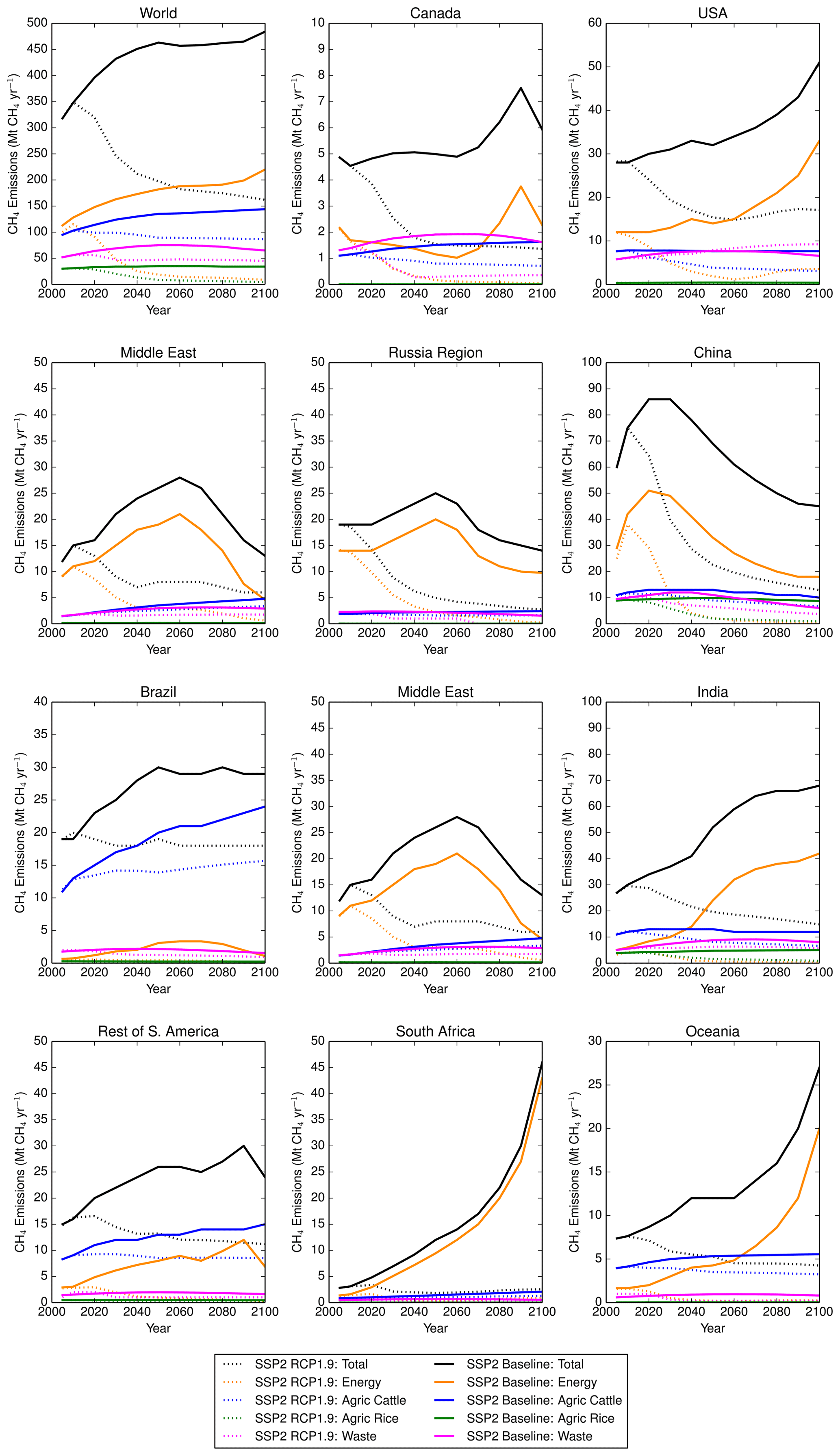
Figure 4 Time series of annual methane emissions between 2005 and 2100 from all and selected anthropogenic sources according to the IMAGE SSP2 Baseline (solid lines) and SSP2-RCP1.9 (dotted lines) scenarios, globally and for selected IMAGE regions, with total emissions in black, energy sector in red, agriculture – cattle in blue, agriculture – rice in green, and waste in magenta. Note that the y axes have different scales for clarity.

2.3.2 Land-based mitigation: baseline, BECCS, and Natural scenarios

For our land-based mitigation scenarios, we take time series of the annual areas assigned to agriculture (crops and pasture) and within that, the area allocated to bioenergy crops, from the IM-BL and IM-1.9 scenarios (defined at the start of Sect. 2.3). We use the dynamic vegetation module in JULES to calculate the evolution of the natural plant functional types and the non-vegetated surface on the remaining land area in the grid cell (see Land use in Sect. 2.1).

The IM-BL LULUC scenario assumes (a) moderate land use change regulation, (b) moderately effective land-based mitigation, (c) the current preference for animal products, (d) moderate improvement in livestock efficiencies, and (e) moderate improvement in crop yields (Table 1 in Doelman et al., 2018). It represents a control scenario within which agricultural land is accrued to feed growing populations associated with the SSP2 pathway and with no deployment of BECCS. Three types of land-based climate change mitigation are implemented in the IMAGE land use mitigation scenarios (Doelman et al., 2018): (1) bioenergy, (2) reducing emissions from deforestation and degradation (REDD or avoided deforestation), and (3) reforestation of degraded forest areas. For the IM-1.9 scenario, there are high levels of REDD and full reforestation. The scenario assumes a food-first policy (Daioglou et al., 2019) so that bioenergy crops are only implemented on land not required for food production (e.g. abandoned agricultural crop land, most notably in central Europe, southern China, and the eastern USA, and on natural grasslands in central Brazil, eastern and southern Africa, and northern Australia; Doelman et al., 2018). The IM-1.9 scenario also requires bioenergy crops to replace forests in temperate and boreal regions (notably Canada and Russia). The demand for bioenergy is linked to the carbon price required to reach the mitigation target (Hoogwijk et al., 2009). In this scenario, the area of land used for bioenergy crops expands rapidly from 2030 to 2050, reaching a maximum of 550 Mha in 2060 and then declining to 430 Mha by 2100. Table 2 gives the maximum area of BECCS deployed in each IMAGE region for the IM-1.9 scenario. This defines the land use in the BECCS scenario.

Table 2 IMAGE regions, the maximum area of BECCS deployed (Mha), and the main differences in land use between the BECCS and Natural scenarios.

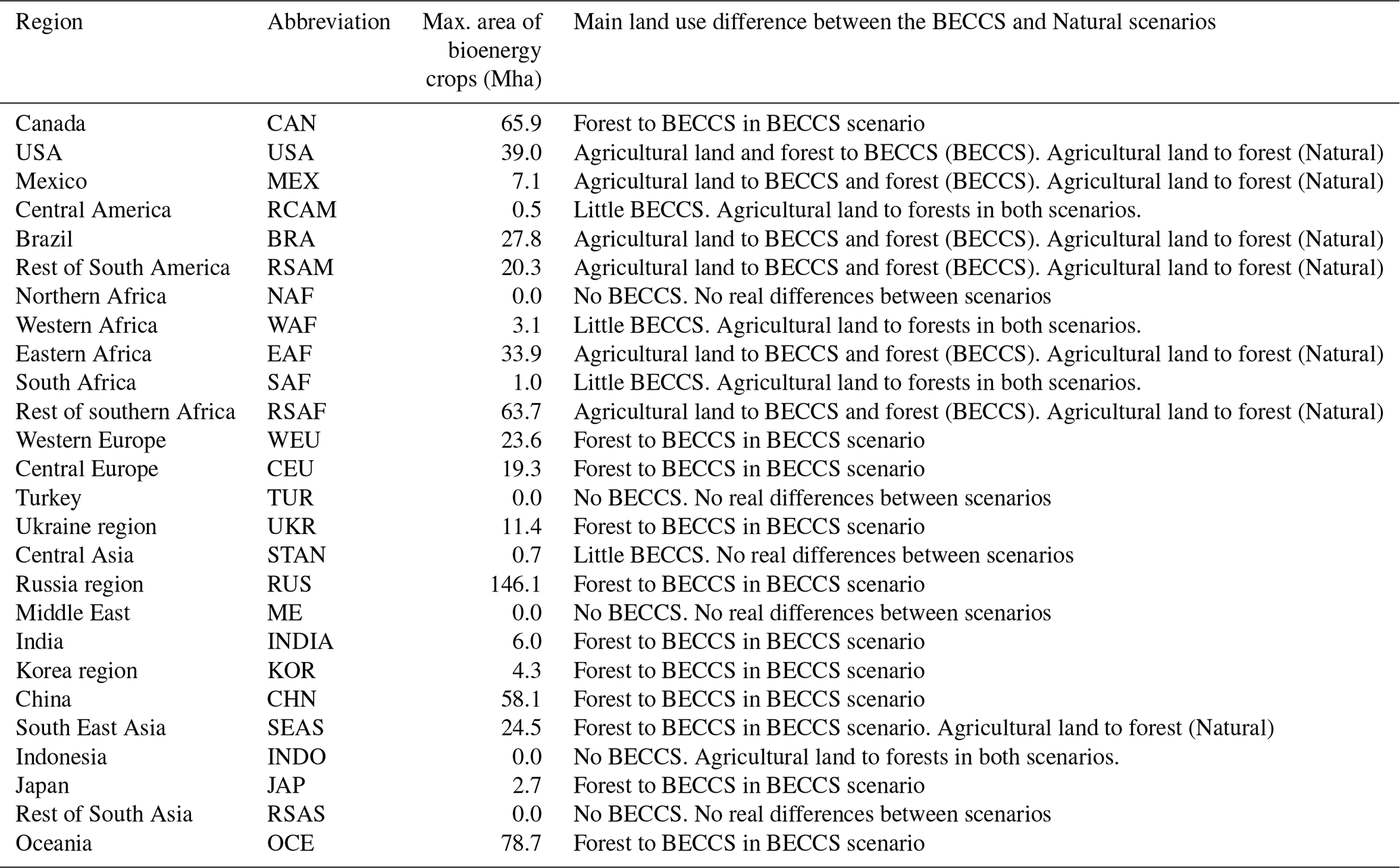
We define a third LULUC pathway, which is identical to the ”BECCS” scenario, except that any land allocated to bioenergy crops is allocated instead to natural vegetation, i.e. areas of natural land, which are converted to bioenergy crops, remain as natural vegetation, and areas that are converted from food crops or pasture to bioenergy crops return to natural vegetation. We make no allowance for any changes in the energy generation system, as this would require energy sector modelling that is beyond the scope of this study. We denote this scenario as Natural. Table 2 also summarises the main differences in land use between the BECCS and Natural scenarios for each IMAGE region.

Figure 5 presents time series of the land areas calculated for trees and prescribed for agriculture (including bioenergy crops) and bioenergy crops for the BECCS and Natural scenarios for the Russia and Brazil IMAGE regions, each as a difference to the baseline scenario (IM-BL). Figure S2 is equivalent to Fig. 5 for all the IMAGE regions.

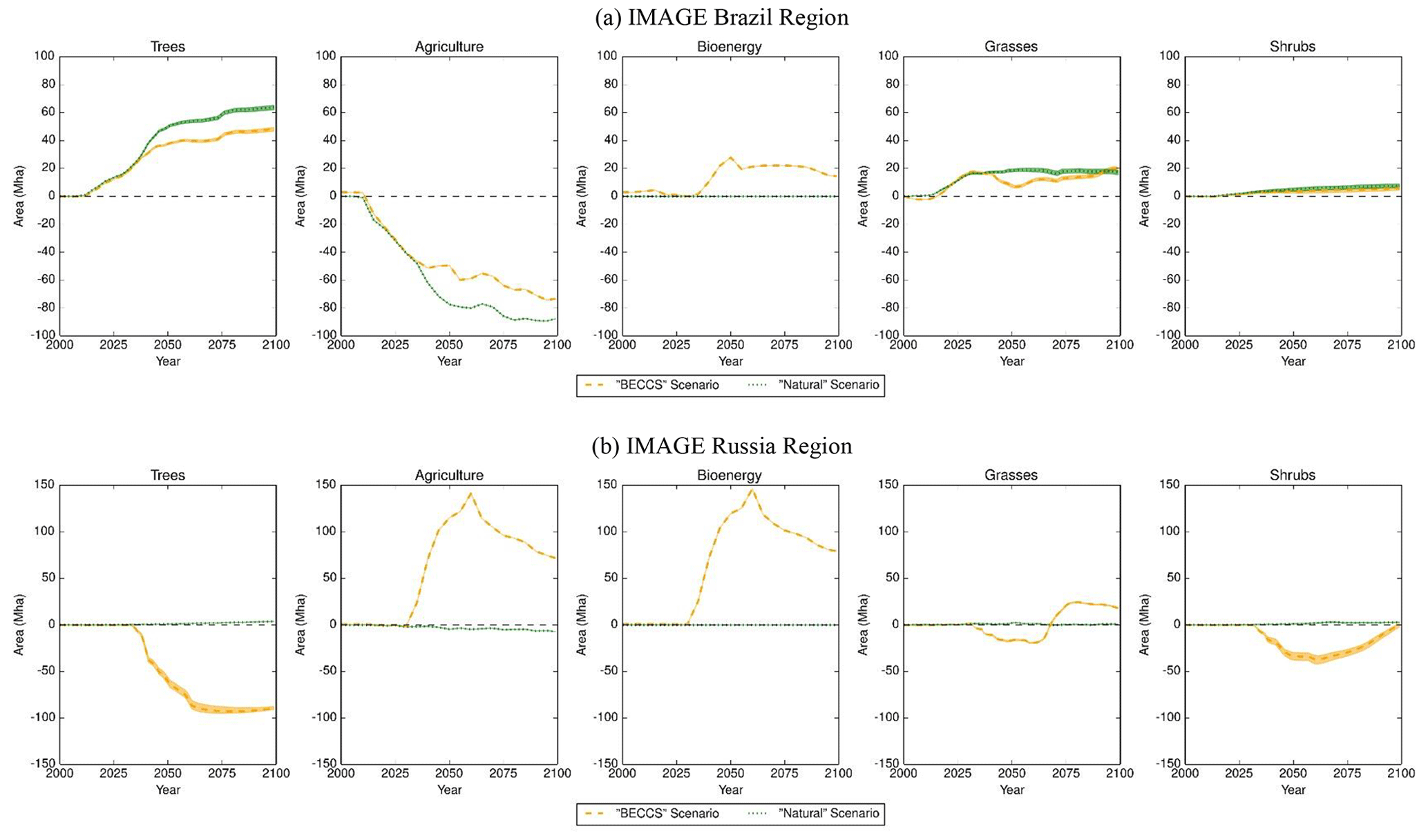
Figure 5 Time series of the land areas (in Mha) calculated for trees and prescribed for agriculture (including bioenergy crops) and bioenergy crops for the BECCS (orange) and Natural (green), as a difference to the baseline scenario (IM-BL), for Brazil (a) and Russia (b) IMAGE regions between 2000 and 2100. The dotted lines are the median and the spread the interquartile range for the 34 GCMs emulated and 4 factorial sensitivity simulations.

2.3.3 Model runs

For each temperature pathway (1.5 or 2.0 ^∘C) and for the baseline and each mitigation scenario, the set of scenario runs comprises a 136-member ensemble (34 GCMs × 2 ozone damage sensitivities × 2 methanogenesis Q₁₀ temperature sensitivities). In all model runs, we include the effects of the methane and carbon–climate feedbacks from wetlands and permafrost thaw, which we have shown previously to be significant constraints on the AFFEBs (Comyn-Platt et al., 2018a).

As shown in Fig. 1, we use a number of input or prescribed datasets: (a) time series of the annual area of land used for agriculture, including that for BECCS if appropriate; (b) time series of the global annual mean atmospheric concentrations of CH₄ (and N₂O for the radiative forcing calculations of CO₂ and CH₄); (c) time series of the overall radiative forcing by SLCFs and non-CO₂ GHGs (corrected for the radiative forcing of CH₄); and (d) time series of annual anthropogenic CH₄ emissions (used in the post-processing step). We take these from the IMAGE database for the relevant IMAGE SSP2 scenario (baseline or SSP2-1.9). Table 1 lists the main scenario runs, their key features and the prescribed datasets used (for agricultural land and BECCS, anthropogenic emissions and atmospheric concentrations of CH₄ and the non-CO₂ radiative forcing).

Figure 6 presents the effect of these scenarios on the modelled atmospheric CH₄ and CO₂ concentrations. We adjust the input atmospheric CH₄ concentrations to allow for the interannual variability in the wetland CH₄ emissions, as described in Sect. 2.2.1. As we use the same input datasets for the two warming targets, the major control on the modelled atmospheric CH₄ concentrations is the CH₄ emission pathway followed, with the temperature pathway (1.5 ^∘C versus 2 ^∘C warming) having a minor effect. For CO₂, on the other hand, the temperature and the CH₄ emission pathways both lead to increased atmospheric CO₂ concentrations, with the temperature pathway having a slightly larger effect.

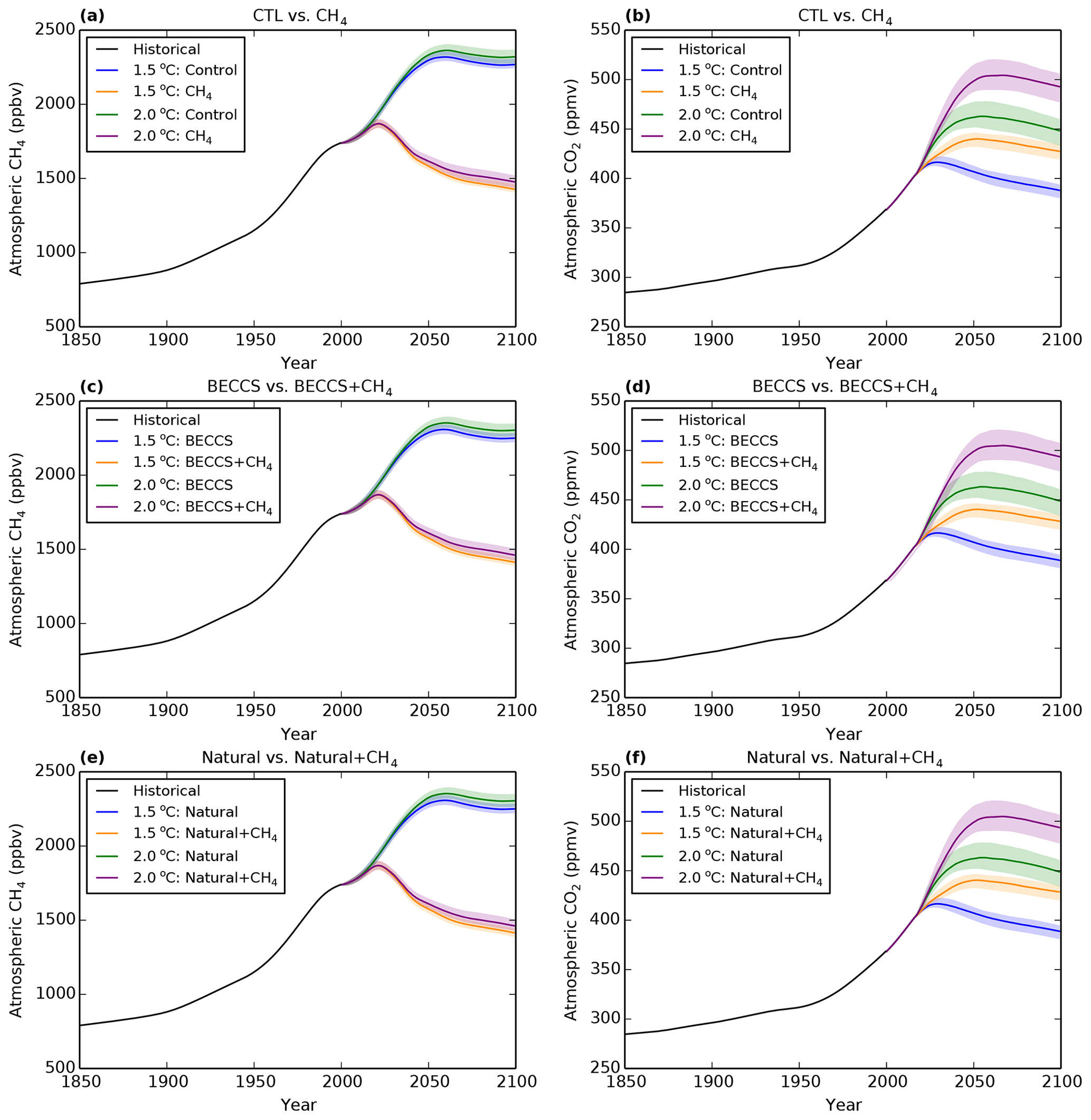
Figure 6 (a, c, e) Time series of the ensemble median atmospheric CH₄ concentrations (with interquartile range as spread) derived for each temperature profile for the following scenarios: (a) CTL and CH₄, (c) BECCS and BECCS + CH₄, (e) Natural and Natural + CH₄. Panels (d, f, h) show the corresponding time series for the atmospheric CO₂ concentrations.

2.4 Post-processing

2.4.1 Anthropogenic fossil fuel emission budget and mitigation potential

Following Comyn-Platt et al. (2018a), we define the anthropogenic fossil fuel CO₂ emission budget (AFFEB) for scenario i as the change in carbon stores from present to the year 2100:

$$\begin{array}{}\text{(7)}& \begin{array}{rl}{\mathrm{AFFEB}}_i& ={\left[C^{\mathrm{land}}\left(\mathrm{2100}\right)-C^{\mathrm{land}}\left(\mathrm{2015}\right)\right]}_i\\ & +{\left[C^{\mathrm{ocean}}\left(\mathrm{2100}\right)-C^{\mathrm{ocean}}\left(\mathrm{2015}\right)\right]}_i\\ & +{\left[C^{\mathrm{atmos}}\left(\mathrm{2100}\right)-C^{\mathrm{atmos}}\left(\mathrm{2015}\right)\right]}_i\\ & +\mathrm{BECCS}(\mathrm{2015}:\mathrm{2100}{)}_i,\end{array}\end{array}$$

where C^land(t), C^ocean(t), and C^atmos(t) are the carbon stored in the land, ocean, and atmosphere, respectively, in year t and BECCS(t₁:t₂) is the carbon sequestered via BECCS between the years t₁ and t₂. The atmospheric carbon store does not include CH₄. This is a reasonable approximation, however, given the relative magnitudes of the atmospheric concentrations of CH₄ (∼2 ppmv at the surface) and CO₂ (400 ppmv).

Within the IMOGEN-JULES modelling framework, we use (a) the IMOGEN climate emulator to derive the changes in the ocean and atmosphere carbon stores and (b) JULES for the changes in the land carbon store and carbon sequestered through BECCS. We discuss the changes in the carbon stores for the baseline and different mitigation scenarios in Sect. 3.1.

For brevity in the subsequent discussion, we use the following shorthand where the terms on the right-hand side of Eq. (7) are equivalent to those on the right-hand side of Eq. (8):

$$\begin{array}{}\text{(8)}& {\mathrm{AFFEB}}_i=\mathrm{\Delta }{C}_i^{\mathrm{land}}+\mathrm{\Delta }{C}_i^{\mathrm{ocean}}+\mathrm{\Delta }{C}_i^{\mathrm{atmos}}+{\mathrm{BECCS}}_i.\end{array}$$

We define the mitigation potential (MP) for a mitigation strategy, j, as the difference between a control AFFEB (AFFEB_ctl) and the AFFEB resulting from applying the strategy, i.e.

$$\begin{array}{}\text{(9)}& {\mathrm{MP}}_j={\mathrm{AFFEB}}_j-{\mathrm{AFFEB}}_{\mathrm{ctl}},\end{array}$$

which can be broken down into its component parts as follows:

$$\begin{array}{}\text{(10)}& \begin{array}{rl}& {\mathrm{MP}}_j={\mathrm{MP}}_j^{\mathrm{land}}+{\mathrm{MP}}_j^{\mathrm{ocean}}+{\mathrm{MP}}_j^{\mathrm{atmos}}\\ & {\mathrm{MP}}_j=\left(\mathrm{\Delta }{C}_j^{\mathrm{land}}-\mathrm{\Delta }{C}_{\mathrm{ctl}}^{\mathrm{land}}\right)+\left(\mathrm{\Delta }{C}_j^{\mathrm{ocean}}-\mathrm{\Delta }{C}_{\mathrm{ctl}}^{\mathrm{ocean}}\right)\\ & +\left(\mathrm{\Delta }{C}_j^{\mathrm{atmos}}-\mathrm{\Delta }{C}_{\mathrm{ctl}}^{\mathrm{atmos}}\right)+{\mathrm{BECCS}}_j.\end{array}\end{array}$$

2.4.2 Optimisation of the land-based mitigation

Harper et al. (2018) find that the land use pathways do not provide a clear choice for the preferred mitigation pathway. The key issue is that replacing natural vegetation with bioenergy crops often results in large emissions of soil carbon and the loss of the benefits of maintaining forest carbon stocks. In such circumstances, Harper et al. (2018) find that the loss of soil carbon in regions with high carbon density makes it difficult for BECCS to deliver a net negative emission of CO₂. Hence, to optimise the land-based mitigation (LBM), we compare the land carbon stocks in the BECCS and Natural scenarios. We then select the optimum land management option for each grid cell simulated as that which maximises the AFFEB by year 2100, i.e.

$$\begin{array}{}\text{(11)}& {\mathrm{AFFEB}}_{\mathrm{LBM}}=\mathrm{\Delta }{C}_{\mathrm{BECCS}}^{\mathrm{atmos}}+\mathrm{\Delta }{C}_{\mathrm{BECCS}}^{\mathrm{ocean}}+\mathrm{\Delta }{C}_{\mathrm{LBM}}^{\mathrm{land}},\end{array}$$

with

$$\begin{array}{}\text{(12)}& \begin{array}{rl}& \mathrm{\Delta }{C}_{\mathrm{LBM}}^{\mathrm{land}}=\\ & \left\{\begin{array}{ll}\sum _l^{\mathrm{grid}\mathrm{cells}}\mathrm{\Delta }{C}_{\mathrm{BECCS}}^{\mathrm{land}}+\mathrm{BECCS}& \mathrm{where}\mathrm{\Delta }{C}_{\mathrm{BECCS}}^{\mathrm{land}}<\mathrm{\Delta }{C}_{\mathrm{BECCS}}^{\mathrm{land}}+\mathrm{BECCS}\\ & \mathrm{or}\\ \sum _l^{\mathrm{grid}\mathrm{cells}}\mathrm{\Delta }{C}_{\mathrm{Natural}}^{\mathrm{land}}& \mathrm{where}\mathrm{\Delta }{C}_{\mathrm{Natural}}^{\mathrm{land}}>\mathrm{\Delta }{C}_{\mathrm{BECCS}}^{\mathrm{land}}+\mathrm{BECCS}\end{array}\right.,\end{array}\end{array}$$

where $\mathrm{\Delta }{C}_{\mathrm{scenario}}^{\mathrm{store}}$ is the change in carbon between 2015 and 2100 for the “store” (= atmosphere, ocean, or land) for the LULUC scenario. We use the ocean and atmosphere contributions from the BECCS simulations as the changes in store size between the BECCS and Natural simulations are negligible (i.e. <2 Gt C).

2.4.3 Assumptions about BECCS efficiency

The efficacy of the BECCS scheme implemented in JULES is significantly lower than that of other implementations (Harper et al., 2018), reflecting the importance of assumptions about the efficiency of the BECCS process and bioenergy crop yields in determining their ability to contribute to climate mitigation. More specifically, there is (1) large uncertainty in carbon losses from farm to final storage (Harper et al. , 2018, assumed a 40 % loss compared to 13 %–52 % loss found in other studies) and (2) a large range in potential productivity of second-generation lignocellulosic bioenergy crops, with JULES falling on the low end. JULES in this study and in Harper et al. (2018) simulated median average yields of ∼4.8 and ∼4.6 tDM ha⁻¹ yr⁻¹ , respectively, compared to measured median of 11.5 tDM ha⁻¹ yr⁻¹ and simulated average of 15.8 tDM ha⁻¹ yr⁻¹ in IMAGE. The JULES yield of ∼4.8 tDM ha⁻¹ yr⁻¹ corresponds to ∼59 EJ yr⁻¹ of primary energy, using the maximum area for BECCS from Table 2 of 637.7 Mha and an energy yield of 19.5 GJ t DM⁻¹ (Daioglou et al., 2017). Bioenergy supplied 55.6 EJ yr⁻¹ or ∼10 % of the primary energy requirement worldwide in 2017 (WBA, 2019). According to Smith et al. (2016), this would increase to ∼170 EJ yr⁻¹ of primary energy in 2100 for negative emissions of 3.3 Gt Ceq yr⁻¹ from BECCS (as required for a 2 ^∘C warming target).

As both of these components are assumed to be diagnostics of the simulations, we can modify the contribution of BECCS to the AFFEB via a post-processing scaling factor, κ, which represents the efficiency of (1) and (2) with respect to the JULES parameterisation. That is, Eq. (12) becomes

$$\begin{array}{}\text{(13)}& \begin{array}{rl}& \mathrm{\Delta }{C}_{\mathrm{LBM}}^{\mathrm{land}}=\\ & \left\{\begin{array}{ll}\sum _l^{\mathrm{grid}\mathrm{cells}}\mathrm{\Delta }{C}_{\mathrm{BECCS}}^{\mathrm{land}}+\mathit{\kappa }\mathrm{BECCS}& \mathrm{where}\mathrm{\Delta }{C}_{\mathrm{Natural}}^{\mathrm{land}}<\mathrm{\Delta }{C}_{\mathrm{BECCS}}^{\mathrm{land}}+\mathit{\kappa }\mathrm{BECCS}\\ & \mathrm{or}\\ \sum _l^{\mathrm{grid}\mathrm{cells}}\mathrm{\Delta }{C}_{\mathrm{Natural}}^{\mathrm{land}}& \mathrm{where}\mathrm{\Delta }{C}_{\mathrm{Natural}}^{\mathrm{land}}>\mathrm{\Delta }{C}_{\mathrm{BECCS}}^{\mathrm{land}}+\mathit{\kappa }\mathrm{BECCS}\end{array}\right..\end{array}\end{array}$$

Figure 7 presents maps of the scaling factor required for BECCS to be the preferable mitigation option, as opposed to natural land carbon uptake, for each grid cell for warming of 1.5 or 2 ^∘C. There are large factors in the northern temperate and boreal regions, parts of Africa, and Australia. As discussed in Harper et al. (2018), this follows from the loss of soil carbon in the tropics and at high northern latitudes leading to long recovery or payback times (10–100+ and >100 years, respectively, Fig. 6c in their paper). The payback time is however insignificant when bioenergy crops replace existing agriculture, for example in Europe and eastern North America.

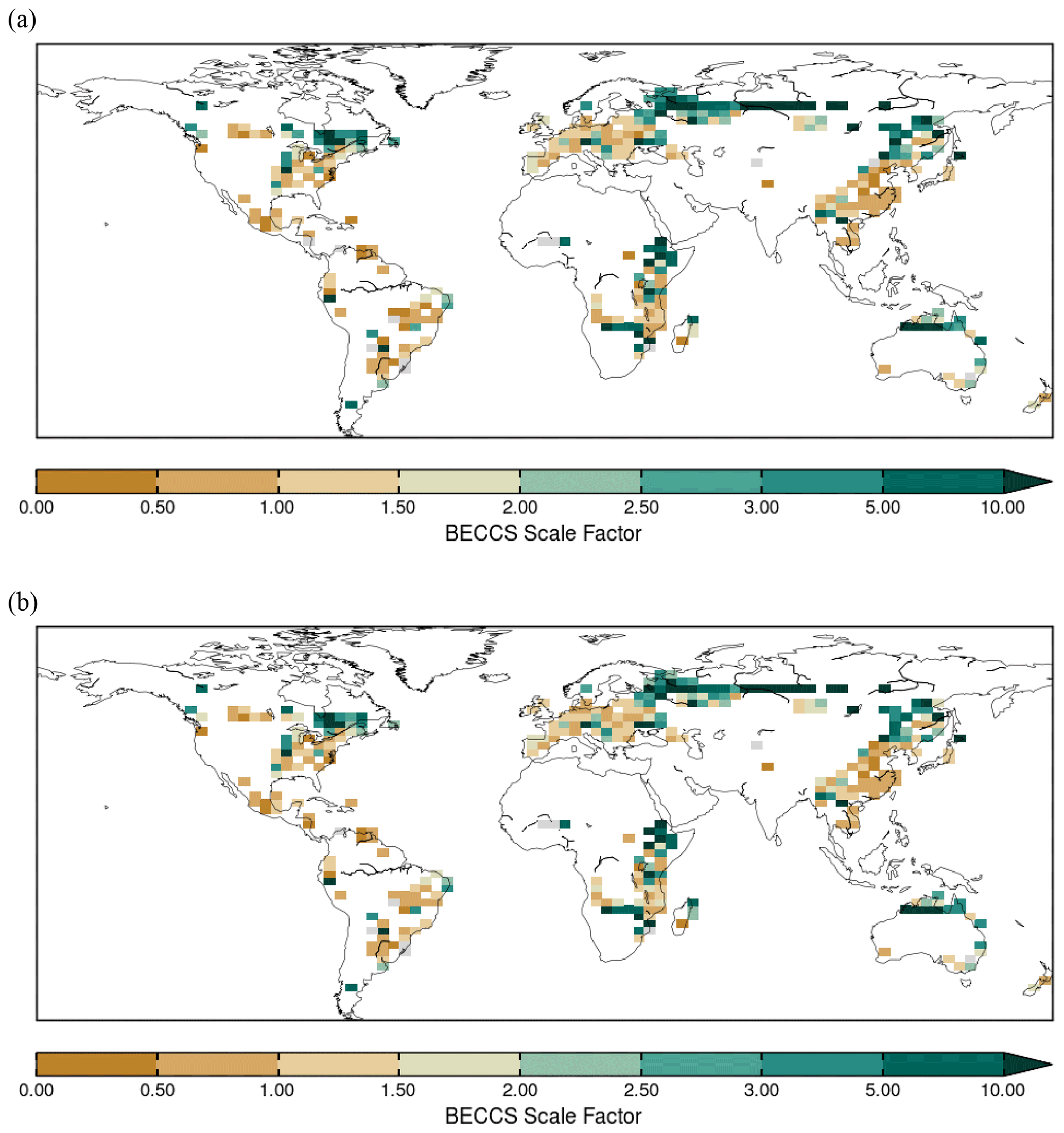
Figure 7 Scale factor required for BECCS to be the preferable mitigation option, as opposed to natural land carbon uptake. The data represents the median of the 136-member ensemble for the optimised land-based mitigation simulation. Panel (a) is for stabilisation at 1.5 ^∘C, and panel (b) is for stabilisation at 2 ^∘C.

Additionally, we define a threshold efficiency factor, κ^*, which represents the required BECCS efficiency for BECCS to be a preferable mitigation strategy for a given grid-cell, i.e.

$$\begin{array}{}\text{(14)}& {\mathit{\kappa }}^{*}={\displaystyle \frac{\mathrm{\Delta }{C}_{\mathrm{Natural}}^{\mathrm{land}}-\mathrm{\Delta }{C}_{\mathrm{BECCS}}^{\mathrm{land}}}{\mathrm{BECCS}}}.\end{array}$$

This increased efficiency can be considered to be the additional bioenergy harvest (H) and/or the reduced carbon losses from farm to storage needed to pay back the carbon debt accrued due to land use change (since carbon removed via BECCS = Hε, where ε is the assumed efficiency factor for farm to storage carbon conservation and H is the simulated biomass harvest). In addition, κ^* implies a new threshold (or break-even) level of BECCS:

$$\begin{array}{}\text{(15)}& {\mathrm{BECCS}}^{*}={\mathit{\kappa }}^{*}\cdot \mathrm{BECCS}.\end{array}$$

In other words, BECCS^* is equivalent to the carbon loss due to the land use change to grow the bioenergy crops. Our IMOGEN-JULES simulations assume a 40 % carbon loss from farm to final storage, although other studies have assumed this to be as low as 13 % (Harper et al., 2018). To assess the feasibility of meeting this break-even level of BECCS, we calculate the harvest (H^*) that would be needed if carbon losses are to be minimised, i.e. by increasing ε from 0.6 to 0.87 and assuming in Eq. (15) that

$${\mathrm{BECCS}}^{*}=\mathrm{0.87}{H}^{*}\mathrm{and}\mathrm{BECCS}=\mathrm{0.60}H,$$

so

$$\begin{array}{}\text{(16)}& H^{*}={\mathit{\kappa }}^{*}\cdot {\displaystyle \frac{\mathrm{0.6}}{\mathrm{0.87}}}\cdot H.\end{array}$$

We discuss this further in Sect. 3.2.

3 Results and discussion

3.1 Global perspective

We calculate the anthropogenic fossil fuel emission budget to limit global warming to a particular temperature target as the sum of the changes in the carbon stores of the atmosphere, land (vegetation and soil), and ocean between 2015 and 2100 (Sect. 2.4.1, Eq. 7 and 8). We use a BECCS scale factor (κ) of unity. In Fig. 8, we present the median and spread of the AFFEB (as box and whiskers) from the 136-member ensemble and the individual GCM and ESM contributions to the AFFEBs from the four carbon pools shown (points) for each of the main scenarios modelled using the IMOGEN-JULES or derived in the post-processing optimisation step (see Table 1 for description of the scenarios).

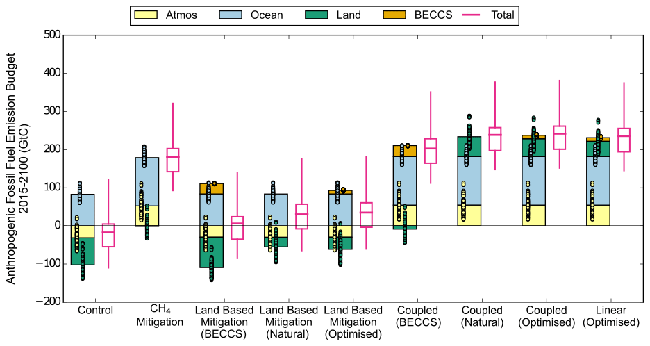
Figure 8 The contribution to the allowable anthropogenic fossil fuel emission budget (AFFEBs, Gt C) from the changes in the different carbon stores (atmosphere, ocean, land, and BECCS) for the various control and mitigation scenarios, illustrated using the temperature pathways for 1.5 ^∘C of warming. The bars are the median of the component 136-member ensembles, with the individual members shown as points. The accompanying pink box and whisker plots to the right of each set of bars are for the AFFEBs (as the sum of the changes in the component carbon stores). The box and whisker plots show the median, interquartile range, minimum, and maximum derived of the resulting AFFEB ensemble. The optimised land-based and coupled mitigation options select the land use option, which maximises the AFFEB for each model grid cell. Note that the land carbon store for the CH₄ scenario at −1.4 Gt C (median of ensemble) is not visible, although the individual ensemble members can be seen as the green points.

In all the scenarios apart from the BECCS scenario, there is an increase in the land carbon store, shown as positive changes for Coupled (Natural) and Coupled (Optimised) but as smaller negative changes for CH₄, Natural, and Optimised scenarios. In the BECCS scenario, the land carbon change becomes more negative than in the CTL scenario, as bioenergy crops replace ecosystems with higher carbon content. In the combined (coupled) CH₄ and land-based mitigation scenarios, the reduction in the emissions and hence atmospheric concentrations of CH₄ allow increased atmospheric concentrations of CO₂ (Fig. 6). There is increased uptake of carbon by the land, directly because of the increased atmospheric CO₂ concentration and indirectly through the reduction in O₃ damage. In the coupled BECCS scenario, this increased uptake of atmospheric CO₂ is again offset by the land carbon lost through conversion of the land to bioenergy crops. We also find that there is increased uptake of CO₂ by the oceans for all scenarios. A further co-benefit of reducing the CH₄ emissions and allowing more CO₂ emissions is that the oceanic drawdown of CO₂ rises (although it eventually falls to zero under climate stabilisation, and there would also be implications for ocean acidification). In Fig. 9a, we compare the AFFEBs for both the 1.5 and 2 ^∘C temperature pathways. We find that the absolute AFFEBs are 200–300 Gt C larger for the 2 ^∘C target than the 1.5 ^∘C target. These budgets are in agreement with other estimates, which include corrections to the historical period (Millar et al., 2017). In both Figs. 8 and 9, it should be noted that the land carbon store for the CH₄ mitigation option at −1.4 Gt C (median of ensemble) is not visible in these figures. There has, however, been a net increase in the land carbon store in the CH₄ scenario when compared to the land carbon store in the control scenario (−70.8 Gt C, median of ensemble). This then explains the positive changes shown for the land carbon stores in the coupled BECCS + CH₄ and coupled Natural + CH₄ scenarios.

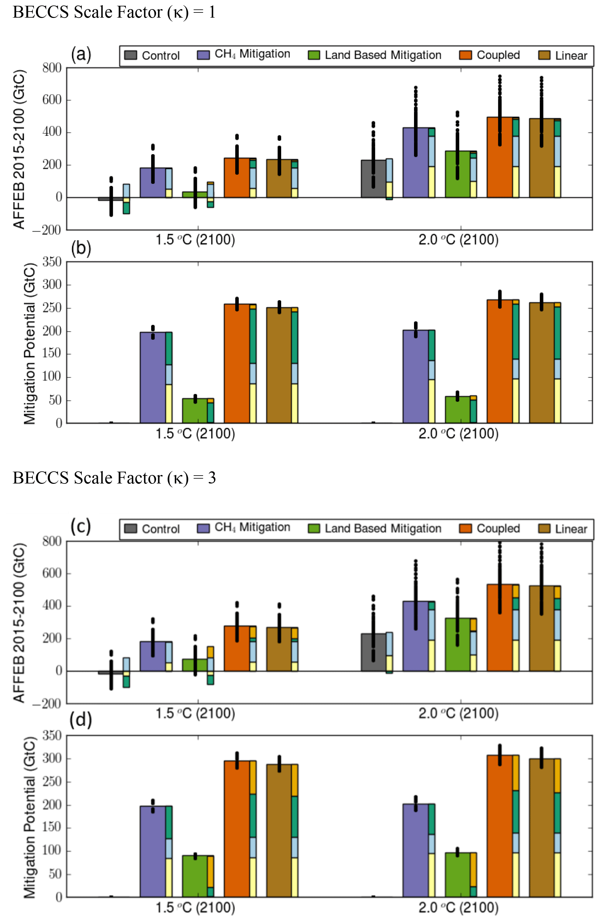
Figure 9 (a, c) The allowable anthropogenic fossil fuel emission budgets (AFFEBs; Gt C) for the control (grey), CH₄ mitigation (purple), land-based mitigation (green), coupled methane and land-based mitigation (orange), and the linearly summed methane and land-based mitigation (brown) for two temperature pathways asymptoting at 1.5 ^∘C (left) and 2.0 ^∘C (right). (b, d) The mitigation potential (Gt C) as the increase in AFFEB from the corresponding control run. The breakdown of each AFFEB and mitigation potential by the changes in the carbon stores is also shown: atmosphere (pale yellow), ocean (light blue), land (dark green), and BECCS (gold) is included alongside each bar. Note that the land carbon store for the CH₄ scenario at −1.4 Gt C (median of ensemble) is not visible. There has, however, been a net increase in the land carbon store in this scenario when compared to the land carbon store in the control run (−70.8 Gt C, median of ensemble).

Figure 9b shows the mitigation potential of each strategy, calculated as the change in the AFFEB from the corresponding control simulation, for the two temperature pathways (Sect. 2.4.1, Eqs. 9 and 10). Methane mitigation is a highly effective strategy: the AFFEBs are increased by 188–206 and 193–212 Gt C for the 1.5 and 2 ^∘C scenarios, respectively, where the range represents the interquartile range from the 136-member ensemble (34 GCMs × 2 Q₁₀ × 2 ozone sensitivities). This AFFEB increase equates to roughly 20–24 years of emissions at current rates for the 1.5 ^∘C target. Land-based mitigation strategies also provide significant increases of 51–57 and 56–62 Gt C for the 1.5 and 2 ^∘C AFFEB estimates, respectively. This is equivalent to 6–7 years of emissions at current rates. For our BECCS assumptions (see also below), we find that the BECCS contribution is small for the optimised land-based mitigation pathway and that AR is a more effective land-based mitigation strategy (Fig. 9b). Although the primary challenge remains mitigation of fossil fuel emissions, these results highlight the potential of these mitigation options to make the Paris climate targets more achievable.

Furthermore, the CH₄ and land-based mitigation strategies show little interaction, and their potential can be summed to give a comparable result to the coupled simulation (coupled vs. linear in Fig. 9a and b). This decoupling is despite the CH₄ emissions from the agricultural sector being influenced by land use choices. We can effectively treat the two mitigation strategies as independent, and their sum approximates the combined potential. Such linearity enables simpler and more direct comparisons.

Despite the substantial differences in the absolute AFFEBs for the 1.5 and 2 ^∘C targets, the mitigation potential of the CH₄ and land-based strategies is similar for the two temperature pathways considered. This similarity suggests that the mitigation strategies are robust to the target temperature; whether the international community aims for the 1.5 or 2 ^∘C target, afforestation, reforestation, reduced deforestation, and CH₄ mitigation are beneficial mitigation approaches.

For both temperature pathways (i.e. 1.5 or 2 ^∘C of warming), we investigate the contribution to the uncertainty range from “climate” as represented by the 34 GCMs emulated and from the land processes investigated (Sect. 2.1). A GCM with higher climate sensitivity will have a lower AFFEB for a specific warming target (and vice versa). In our post-processing steps, we derive a number of statistical parameters from the complete 136-member or 34-member GCM ensemble for the individual factorial runs (low Q₁₀/low O₃, low Q₁₀/high O₃, high Q₁₀/low O₃, and high Q₁₀/high O₃), such as mean, standard deviation, median, and various percentiles. Our focus is on the contribution different factors make to the overall standard deviation of the 136-member ensemble (σ_All). By factoring out the climate variation (via their means), we calculate the standard deviation for the land processes investigated (σ_land). With a knowledge of the overall standard deviation and that for land-only processes, we derive the contribution from “climate” (σ_climate) assuming that the variances are independent and can be summed (Eq. 17). The contributions of uncertainty found are by comparing ratios of σ_land to σ_climate.

$$\begin{array}{}\text{(17)}& {\mathit{\sigma }}_{\mathrm{all}}^{\mathrm{2}}={\mathit{\sigma }}_{\mathrm{climate}}^{\mathrm{2}}+{\mathit{\sigma }}_{\mathrm{land}}^{\mathrm{2}}\end{array}$$

We present the results of this analysis in Table 3 for the Anthropogenic Fossil Field CO₂ Emission Budgets and the Mitigation Potential (= scenario – CTL) for the 1.5 ^∘C temperature profile (Table S2 is equivalent table for the 2 ^∘C temperature profile). Our overall finding is that the climate uncertainty dominates the uncertainty of the AFFEBs. However, when considering different trade-offs between land uncertainty and mitigation options, the impact of climate uncertainty is much weaker. Within the land uncertainty, the O₃ vegetation damage appears to make the greater contribution (from the changes in the mean). Although there is some variation in the ratio (σ_climate:σ_land) between the scenarios (0.32±0.13, mean ± standard deviation), this gives us confidence in the robustness of the uncertainty estimates derived across the scenarios and the two temperature profiles.

Table 3 For the 1.5 ^∘C temperature profile, the mean of the 34-GCM member ensembles for the CTL and mitigation scenarios for the different factorial runs (low Q₁₀/low O₃, low Q₁₀/high O₃, high Q₁₀/low O₃ and high Q₁₀/high O₃), the standard deviation of the full 136-member ensemble (Gt C), the derived standard deviations for land processes (σ_land) and climate (σ_climate, as represented by the 34 GCMs) and the ratio of ${\mathit{\sigma }}_{\mathrm{climate}}/{\mathit{\sigma }}_{\mathrm{land}}$ for (a) the Anthropogenic Fossil Field CO₂ Emission Budgets and (b) the Mitigation Potential (= scenario − CTL).

3.2 Sensitivity to BECCS efficiency

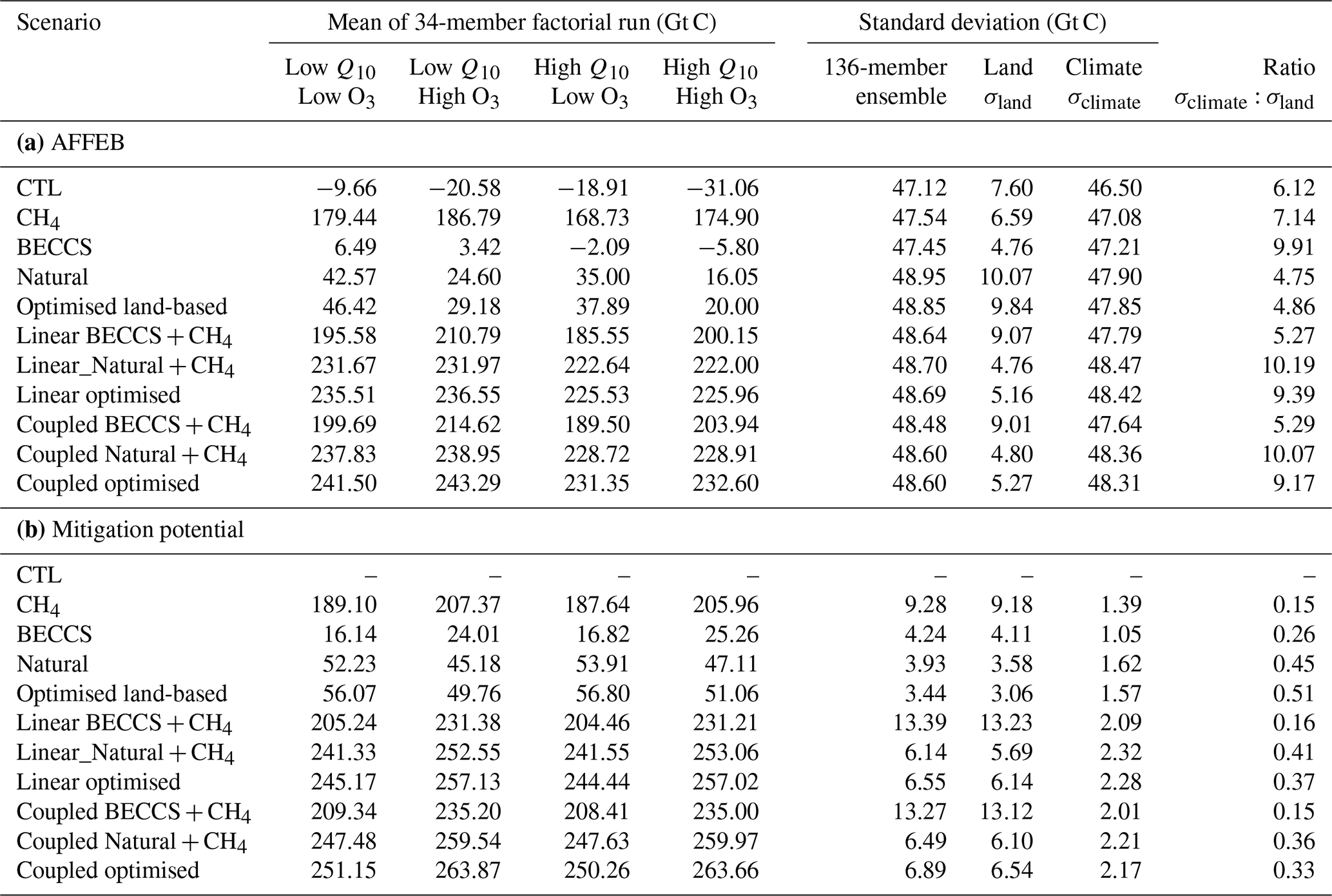
The BECCS parameterisation used here makes BECCS less effective compared to those in other studies (van Vuuren et al., 2018). Globally across the two temperature targets, our simulations imply a removal of 27–30 Gt C from the active carbon cycle via BECCS in the original BECCS scenario run, which is reduced to ∼7–12 Gt C after we optimise the land use scenario. These removal rates are significantly lower than other estimates based on the same land use scenarios: 73 Gt C in a similar dynamic global vegetation model (LPJ-GUESS) and 130 Gt C in IMAGE (Harper et al., 2018). We find that doubling the carbon captured with BECCS in our simulations (Sect. 2.4.3, κ=2) has a relatively small impact on the total mitigation potential in the optimised scenario (Fig. 10a). This low sensitivity is because the increased carbon removed by BECCS often accompanies a comparable decrease in the carbon uptake from the “natural” vegetation that it replaces. It is only when setting the BECCS carbon sequestration at 3–5 times its original value that there is a notable increase of the global AFFEB. Further, as shown in Fig. 10b, there is reduction in soil carbon in specific regions (e.g. northern temperate and boreal regions), which makes BECCS less effective for carbon sequestration than natural land management options (or there is a long payback time, as discussed in Harper et al., 2018).

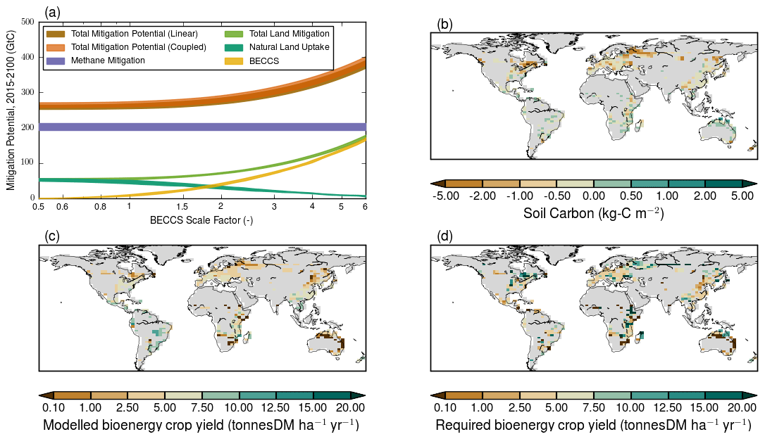
Figure 10 (a) The total and component mitigation potential (Gt C) for different mitigation options, involving methane and land use, as a function of the BECCS efficiency factor (κ, Sect. 2.4.3) for the temperature pathway reaching 1.5 ^∘C. The width of the lines represent the interquartile range of the 136-member ensembles. Maps of (b) the change of the modelled soil carbon (kg C m⁻²) between 2015 and 2099, as the difference between the scenario with BECCS and the natural land-management scenario; (c) the modelled mean bioenergy crop yield in the JULES simulations (κ=1); and (d) the required bioenergy crop yield for BECCS to provide a larger carbon uptake than forest regrowth and afforestation (assuming $\mathit{\kappa }={\mathit{\kappa }}^{*}$ and 87 % efficiency of BECCS). Grid cells that do not exceed 1 % BECCS cover for any year in the simulation are masked grey.

Increased carbon removal with BECCS could be realised through either (1) minimising the loss of carbon from farm to final storage (ε in Sect. 2.4.3) or (2) maximising the productivity of the bioenergy crop. Our IMOGEN-JULES simulations assume a 40 % carbon loss from farm to final storage, although other studies have assumed this to be as low as 13 % (Harper et al., 2018). The bioenergy crop yields in JULES (Fig. 10c) are lower than the median yield of Miscanthus (11.5 t of dry matter (t DM) ha⁻¹ yr⁻¹), as measured from 990 mostly European plots (Li et al., 2018), and are about half the productivity of those in the IMAGE simulations. We calculate for each IMOGEN grid cell the increase in carbon removed via BECCS and the associated increase in bioenergy crop yields (H^* in Sect. 2.4.3) required for BECCS to be the preferred mitigation option (Fig. 10d), rather than natural land carbon uptake, and assuming minimal amounts of carbon are lost during the BECCS life cycle (13 % carbon loss). In many places, we find that the required yield increases from <10 to 10–20 t DM ha⁻¹ yr⁻¹ are achievable but that required yields of >30 t DM ha⁻¹ yr⁻¹ would be more difficult to realise, given the range of yields observed (Li et al., 2018). We provide additional information in Table S4a–d on the modelled bioenergy yields and the yields required for bioenergy crops to be the preferred land-based mitigation option by IMAGE region. The tables also show that area of bioenergy crops and carbon sequestered by BECCS increases, as expected, with the BECCS scale factor (κ).

We conclude that our uncorrected simulations are a lower estimate for the potential of carbon removal via BECCS. We provide a more optimistic estimate of the BECCS potential using κ=3, which results from doubling the JULES yields and increasing the efficiency ε from 0.6 to 0.87 (i.e. $\mathit{\kappa }\sim \mathrm{2}\times \mathrm{0.87}/\mathrm{0.6}$). We now find the global land-based mitigation potential to be 88–100 Gt C across the two temperature targets, as shown in Fig. 9c and d. Figure S3 shows the corresponding plots for the 2 ^∘C warming target. We use κ=3 in the subsequent analysis of regional mitigation options and of BECCS water requirements.

3.3 Regional analysis

We consider the sub-continental implications of CH₄ and land-based mitigation options, using the 26 regions of the IMAGE model (Stehfest et al., 2014). Figure 11 shows the contributions of the three mitigation options – CH₄, carbon uptake through AR, and BECCS – to the AFFEBs for each IMAGE region and for the temperature pathway stabilising at 1.5 ^∘C.

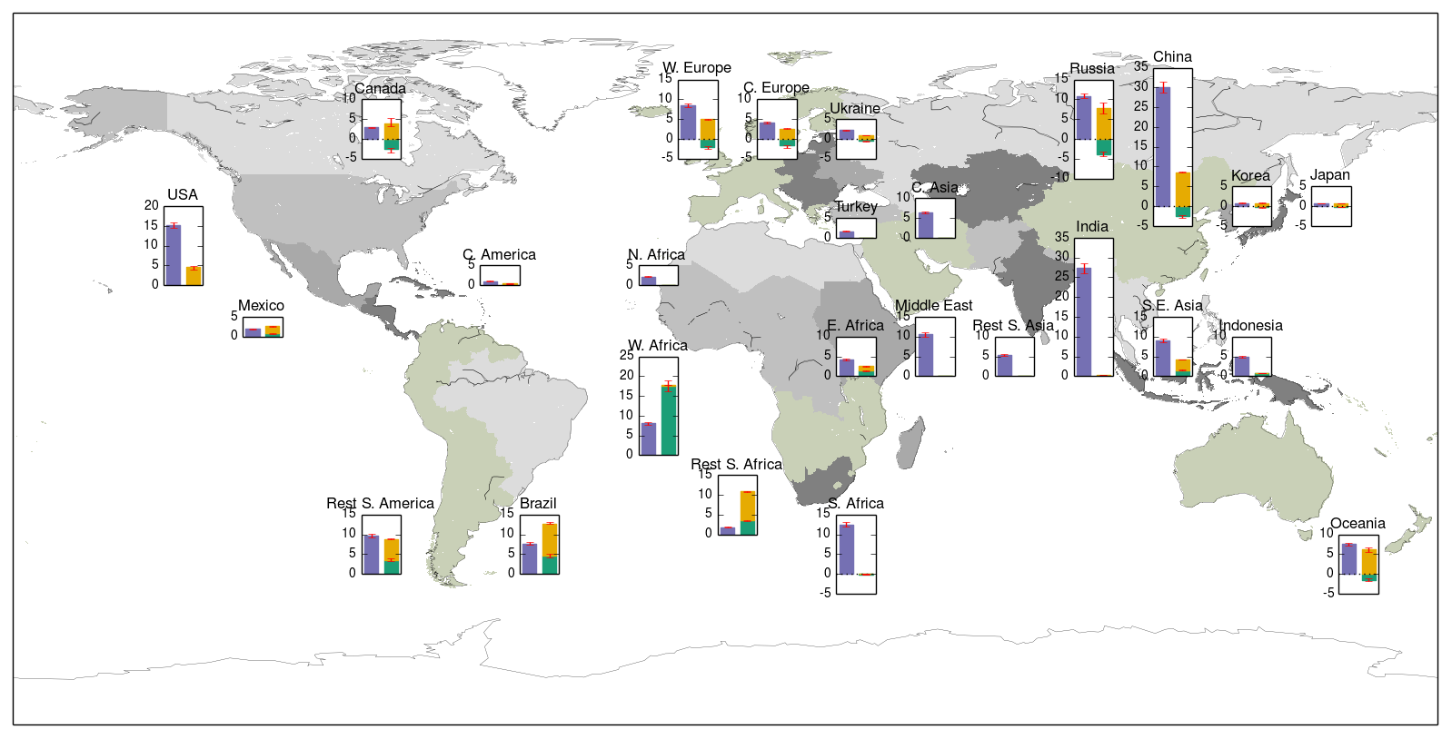
Figure 11 The contribution to the allowable carbon emission budgets (Gt C) between 2015 and 2100 for each of the 26 IMAGE IAM regions from methane mitigation (purple bars) and land-based mitigation options (green: natural land uptake; yellow: BECCS with κ=3) for the temperature pathway stabilising at 1.5°warming without overshoot. The bars and error bars show the median and the interquartile range, respectively, from the 136-member ensembles.

We estimate the regional land-based mitigation as the change in the land carbon stores plus the carbon removal via BECCS for each IMAGE region in the IMOGEN-JULES model output. In this accounting, the region where the bioenergy crops are grown is credited with the carbon removal via BECCS. We assume a 3-fold increase in carbon removal via BECCS compared to our default simulations (κ=3) to highlight regions where BECCS is potentially viable. Figure 12 shows the sensitivity of the global AFFEBs and mitigation potential for κ=1, 2, and 3 for 1.5 ^∘C of warming (Fig. S3 is the corresponding figure for 2 ^∘C of warming). For CH₄, we use regional-scale factors to allocate changes in the global atmospheric CH₄ concentration, and therefore the CH₄ mitigation potential, to each region, as shown in Table S3. To derive the regional-scale factors, we separately sum the projected anthropogenic CH₄ emissions between 2020 and 2100 between the IMAGE SSP2-Baseline and SSP2-1.9 scenarios (van Vuuren et al., 2017). We calculate the scale factor as the regional fraction of the global difference in the summed emissions (Table S3). These two CH₄ scenarios are consistent with the CH₄ concentration pathways considered in the CH₄ scenario simulations (Sect. 2.3). We use the scale factors to produce Figs. 11 and 12 (and Figs. S3 and S4).

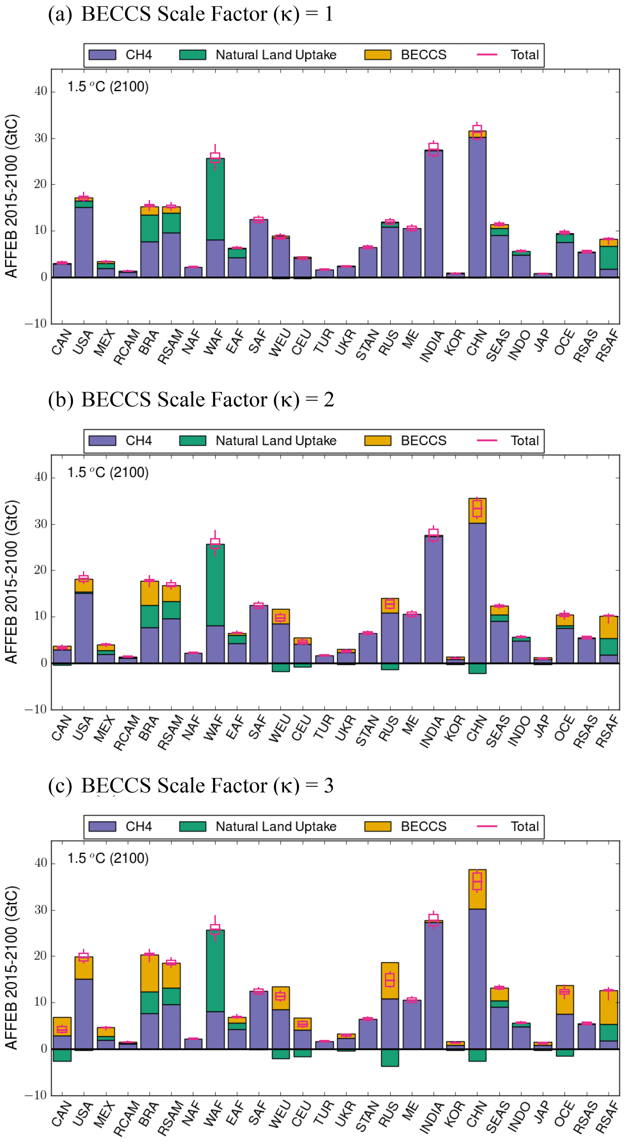
Figure 12 Contribution of different mitigation options to the increase in allowable anthropogenic fossil fuel emission budgets by IMAGE region to meet the 1.5 ^∘C target. The stacked bars represent the median methane mitigation potential (purple bars) and median land-based mitigation potential (natural land uptake, green; BECCS, brown). Panel (a) is based on a BECCS scaling factor of unity, panel (b) a BECCS scaling factor of 2, and panel (c) a BECCS scaling factor of 3. The total (pink) shows the median and interquartile range of the 136-member ensembles.

CH₄ mitigation is an effective mitigation strategy for all regions, and especially the major methane emitting regions: India, southern Africa, the USA, China, and Australasia. Figure 4 presented time series of the anthropogenic CH₄ emissions for selected IMAGE region from 2000 to 2100 (and Fig. S1 presents emission time series for all IMAGE regions). The mitigation of CH₄ emissions from fossil fuel production, distribution and use for energy is the largest contributor for India, southern Africa, the USA, China, and Australasia. The emissions from agriculture relating to cattle (for India, USA and China) and rice production (China and other Asian regions) make smaller contributions.

The impact of the land-based mitigation options links strongly to the managed land use and land use change (LULUC). As discussed in Sect. 2.3.2, we list in Table 2 the maximum area of BECCS deployed in each IMAGE region and the main differences in land use between the BECCS and Natural scenarios. Figure 5 presents time series of the land areas calculated for trees and prescribed for agriculture (including bioenergy crops) and bioenergy crops for the BECCS and Natural scenarios for the Russia and Brazil IMAGE regions, each as a difference to the baseline scenario (IM-BL) (see Fig. S2 for all the IMAGE regions). The West Africa region shows the largest natural land carbon uptake (WAF in Fig. 12). Here, there is conversion of crop and pasture to forest, with little land used for bioenergy crops for BECCS. For Brazil (Fig. 5a) and the rest of South America, both bioenergy crops and forest expand at the expense of agricultural land. For many other regions, notably Canada, Russia, western and central Europe, China, and Oceania, there is less carbon uptake from the “land” in the optimised mitigation scenario, even though the overall carbon uptake has increased. For Canada and Russia, this results from the loss of forest in the BECCS land use scenario (see Figs. 5b and S3). The carbon uptake by BECCS increases as κ increases from 1 to 3 because there are more grid cells where “BECCS” is the preferred mitigation option in the optimisation process, as evidenced by the increase in area of bioenergy crops (Table S4a and c). As κ only affects the “BECCS” term (Sect. 2.4.3, Eq. 13), the increased carbon removed by BECCS is often accompanied by a decrease in the carbon uptake from the “natural” vegetation that it replaces. This can be seen more clearly in Fig. 12 (and Fig. S3 for 2 ^∘C warming) and Table S4b and d. The version of JULES used in this study currently lacks a fire regime. There will be risks to long-term storage of carbon stored in vegetation in regions with significant areas of fire-dominated vegetation cover (e.g. savannah in Brazil and Africa). Further, this version of JULES does not include a nitrogen cycle, which has been implemented in more recent versions of the model. This will enable the impact of changes in land use and agriculture on N₂O emissions to be integrated into the assessments.

There is relatively little difference in the additional allowable carbon emission budgets introduced by CH₄ and/or the land-based mitigation between 2015 and 2100 for the two temperature pathways considered (Fig. S4 for the contributions at 2 ^∘C of warming).

3.4 Water resources

Smith et al. (2016) estimate the global water requirements for different negative emission technologies, including BECCS. We also derive the water requirements from the carbon uptake by BECCS for our optimised land-based mitigation scenarios. The IM-1.9 land use scenario (Sect. 2.3.2) assumes that bioenergy crops are grown sustainably and are rain-fed (Daioglou et al., 2019; Hoogwijk et al., 2005). Our land surface modelling system explicitly accounts for this. We derive the additional water requirements for BECCS, using κ=3 and assuming (a) a marginal increase in water use of 80 m³ (tC eq)⁻¹ yr⁻¹ when replacing the average short vegetation (i.e. ${\mathrm{C}}_{\mathrm{3}}/{\mathrm{C}}_{\mathrm{4}}$ grasses in JULES) by a biomass energy crop (Smith et al., 2016) and (b) 450 m³ (tC eq)⁻¹ yr⁻¹ for the CCS component (Smith et al., 2016).

Following Postel et al. (1996), we derive the accessible runoff, using their assumptions that only 5% of the total runoff is geographically and/or temporally accessible for the Brazil, Russia, and Canada IMAGE regions and that 40 % is accessible elsewhere. Our present-day estimates of the global annual runoff (43 000–44 200 km³ yr⁻¹) and the accessible runoff for human use (11 400–11 720 km³ yr⁻¹) (see Fig. 13) are both in agreement with the values given in Postel et al. (1996), i.e. total and accessible runoffs of 40 700 and 12 500 km³ yr⁻¹, respectively.

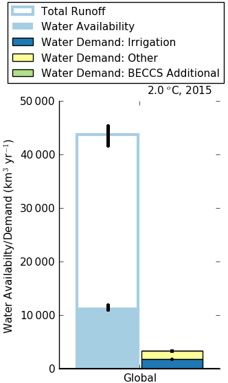
Figure 13 Global water availability (filled light blue bar) as a regionally dependent fraction of runoff (hollow light blue bar) for the year 2015. The water demand for irrigation (dark blue) and for other uses (i.e. energy generation, industry, and domestic; yellow) are taken from the SSP2-RCP2.6-IMAGE database. Note that there is very little BECCS additional water demand (green) in 2015.

We use the water withdrawals for each IMAGE region given in the IMAGE-SSP2-RCP2.6 scenario for the water demand for agricultural irrigation (Rost et al., 2008) and for other human activities, such as energy generation, industry, and domestic usage (Bijl et al., 2016) between 2015 and 2100 (Table 4a and b). We assume the same water demands from these sectors for both the 1.5 and 2 ^∘C warming targets.

Table 4 (a) Comparison by IMAGE region of the modelled available water (km³ yr⁻¹), the projected water withdrawals (km³ yr⁻¹) for irrigation and for other anthropogenic activities (energy generation, industry, domestic) from the IMAGE SSP2-RCP2.6 scenario, and the additional water required for BECCS (km³ yr⁻¹ and as percentages of the net available water and of the water withdrawals for irrigation and other) for the year 2060. The percentage of runoff available for human use by IMAGE region is also included. Section (b) is the same as (a) but for 2100.

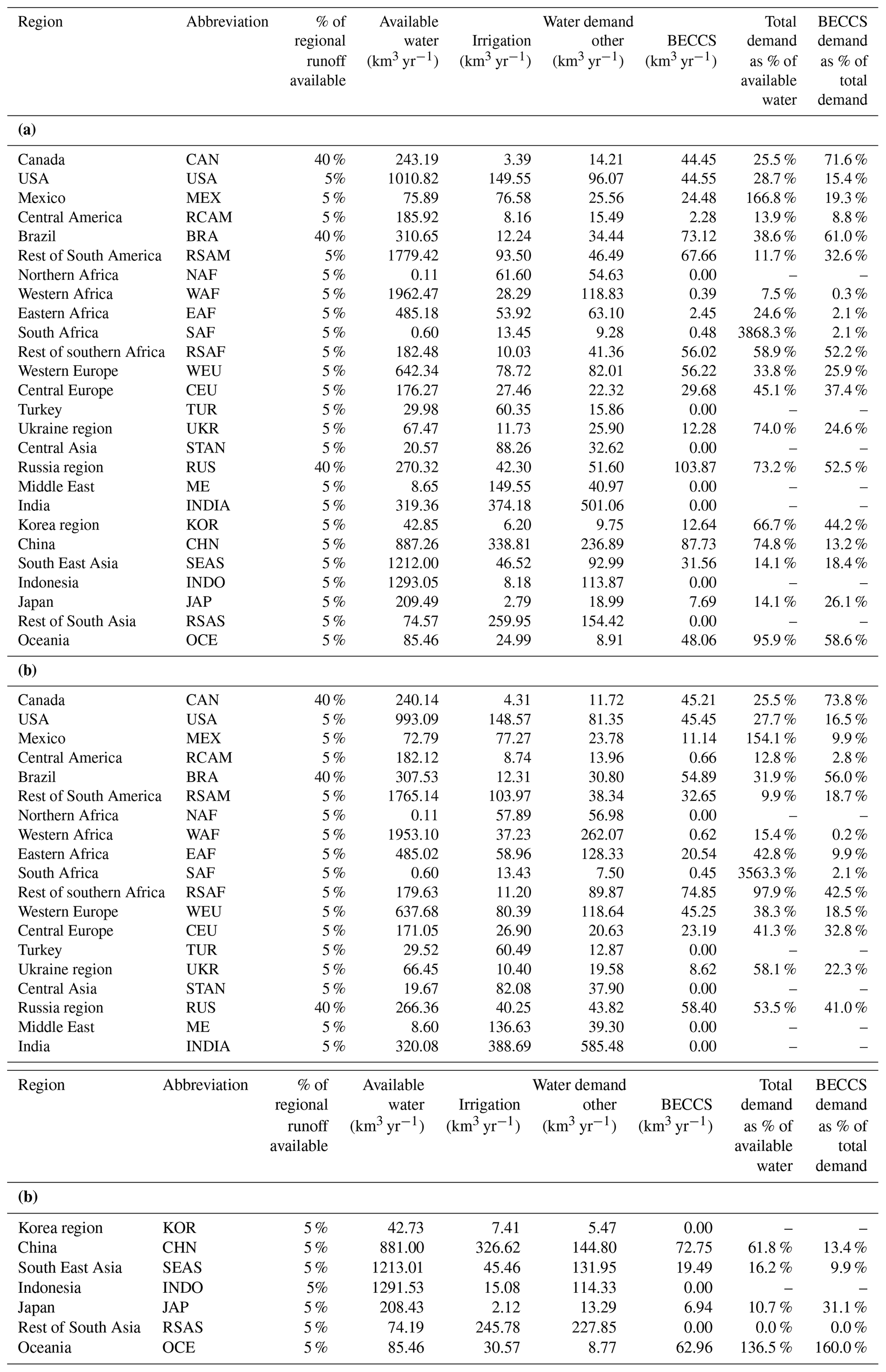
Figure 14 compares the accessible water with the water demand for BECCS and other human activities for the regions that produce a substantial amount of BECCS, Canada, USA, Brazil, Europe, Russia, China, southern Africa, and Oceania, for the optimised land-based mitigation. Table 4a and b show the additional water requirements of BECCS calculated for 2060 and 2100, respectively, for the 2 ^∘C warming target. We find that the additional demand for BECCS would lead to an exceedance (or use >90 %) of the available water for the Oceania and rest of southern Africa regions. We also find that the additional demand for BECCS is greater than the total water withdrawals from anthropogenic activities for the Canada and Brazil IMAGE regions. Our estimates represent a maximum possible water usage for BECCS as (i) the SSP2 scenario used already accounts for the lower power generation efficiencies and hence higher water requirements in switching from fossil fuels to bioenergy crops, which could be up to 20 %–25 %, and (ii) the figure used for the CCS component does not allow for future technological improvements in water use. For example, Fajardy and Mac Dowell (2017) indicate a 30-fold reduction in water use when changing from a once-through to a recirculating cooling tower. Our results are less severe than other studies considering BECCS water requirements (Séférian et al., 2018; Yamagata et al., 2018) because the carbon removed by BECCS in this study (30 Gt C) is already limited to regions where it is more beneficial to the AFFEB than forest-based mitigation options. We also note from Bijl et al. (2016) that the water demand for irrigation, derived using the coupled IMAGE-LPJmL models, is low compared to other estimates in the literature. Higher water demand for irrigation existing agriculture would be an additional constraint on the water available for BECCS. Nevertheless, our results indicate that the additional water demand for BECCS would have large impacts in half of the regions substantially invested in BECCS: Oceania, rest of southern Africa, Brazil, and Canada.

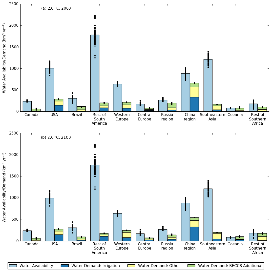
Figure 14 Water availability (light blue), SSP2-IMAGE water demand estimates for irrigation (dark blue), other uses (i.e. energy generation, industry, and domestic; yellow), and the additional water demand from BECCS (green) for the years 2059–2060 and 2099–2100 for the 2.0 ^∘C warming target, with a BECCS κ factor of 3. The points are the individual results from the 136-member ensembles, while the bars are the corresponding median values of the ensembles.

4 Conclusions

Our paper brings together previous studies that looked separately into the potential of methane mitigation (Collins et al., 2018) and land management options (especially forest conservation and BECCS) (Harper et al., 2018), into a single unified framework. Uniquely, this allows us to compare these options at local and regional scales. We utilise the detailed JULES land surface model, which includes methane production from wetlands and permafrost thaw (Comyn-Platt et al., 2018a) and the effect of CH₄ emissions on land carbon storage via ozone impacts on vegetation (Sitch et al., 2007), and we also span the range of climate model projections using the IMOGEN ESM emulator. For each temperature pathway and each of the three mitigation options, the set of scenario runs comprises a 136-member ensemble (34 GCMs × 2 ozone damage sensitivities × 2 methanogenesis Q₁₀ temperature sensitivities).

This analysis quantifies the regional differences in potential CH₄ and/or land-based strategies to aid mitigation of climate change. We present our findings within a full probabilistic framework, capturing uncertainty in climate projections across the CMIP5 ensemble, as well as process uncertainties associated with the strength of natural CH₄ climate feedbacks from wetlands and ozone-induced vegetation damage. Globally, mitigation of anthropogenic CH₄ emissions and the optimised land-based mitigation can potentially offset (i.e. allow extra) fossil fuel carbon dioxide emissions of 188–212 and 51–100 Gt C, respectively. These bounds are almost independent of the eventual global warming target or the climate sensitivity of the climate models emulated. As shown in Sect. 3.1, the CH₄ and land-based mitigation strategies show little interaction and their potential can be summed to give a comparable result to the corresponding coupled simulation. This decoupling is despite the CH₄ emissions from the agricultural sector being influenced by land use choices. We can therefore treat the two mitigation strategies as independent and sum their individual potentials. Such linearity enables simpler and more direct comparisons between the carbon budgets of methane and land-based mitigation strategies. However, some caveats remain. Land surface models still require refinement, alongside improved characterisation of the assumptions inherent in the socio-economic pathways and IAM modelling. Further, we do not allow for the reduced emissions from fossil fuel combustion due to the bioenergy crop being grown (or the converse when bioenergy crops are replaced in the Natural model run), as this would require energy sector modelling that is beyond the scope of this study.

For the Natural land-based scenario (see Table  1), we find a mitigation potential of 50–55 Gt C (183–201 Gt CO₂). The land-based mitigation estimates vary over wide ranges, partly related to different assumptions on land use and carbon pools. Our results are within the wide range of the overall deployment of CO₂ removal by agriculture, forestry, and other land use (including afforestation and reforestation) to 2100 of 200 [0–550] Gt CO₂ (in IPCC, 2018, p. 2.40) and of estimates of the cumulative potential to 2100 from 80 to 260 Gt CO₂ (Table 2) in Minx et al. (2018). In the BECCS scenario, we obtain a geological carbon storage via BECCS (27±1 Gt C median, interquartile range) similar to that (30±1 Gt C) derived by Harper et al. (2018), for the same land use scenario (IM-1.9). Our result is lower as we include the natural methane feedbacks from wetlands and permafrost thaw. Inclusion of this better process description leads to ∼10 % reduction in carbon budgets (Comyn-Platt et al., 2018a). These estimates for the geological carbon storage via BECCS are much lower than the corresponding value derived by the IMAGE IAM (130 Gt C). Harper et al. (2018) discuss this difference, identifying a number of reasons for the lower value: the use of initial above-ground biomass harvested in boreal forests for BECCS; the replacement of fossil-fuel-based emissions in the energy system; and specific assumptions about crop yields, conversion efficiency, use of residues, and the proportion of bioenergy crops used with CCS. Estimates of the BECCS contribution in the literature vary over a wide range (from 178 to >1000 Gt CO₂, according to Minx et al., 2018), but in recent studies these results are typically revised downwards taking into account among others sustainability constraints (e.g. Fuss et al. (2018) suggests a potential of 0.5–5 Gt CO₂ per year in 2050).

We investigate the efficacy of our BECCS scenario by increasing the productivity of BECCS (using a scale factor κ). From comparison with observed bioenergy crop yields, we argue that the scale factor could be between 1 and 3. We highlight how using this range of κ provides characterisation of an additional source of uncertainty on the land-based mitigation potential. In our optimised land-based mitigation scenario, which maximises the land carbon uptake (Sect. 2.4.2, Eq. 13), the increased carbon removed by BECCS is often accompanied by a decrease in the carbon uptake from the “natural” vegetation that it replaces (as discussed in Sect. 3.3 and shown in Fig. 12). This concern is equivalent to the statement in Harper et al. (2018) that the “use of BECCS in regions where bioenergy crops replace ecosystems with high carbon contents could easily result in negative carbon balance”. Hence, the particularly novel feature of our paper is that our optimal approach accounts explicitly for that trade-off, only suggesting BECCS where there is a net gain. For boreal forest regions there is a preference for avoided deforestation, whereas in tropical forest regions both AR and avoided deforestation offer significant potential. From a carbon sequestration perspective, growing bioenergy crops for BECCS is only preferable where it replaces existing agricultural land. BECCS has particular potential if productivities and power production efficiencies are towards the upper limit of expected photosynthetic capability, whilst noting the strong water demand of such crops requires consideration in the context of a growing population.

Stabilising the climate primarily requires urgent action to mitigate CO₂ emissions. However, we estimate that CH₄ mitigation may offset up to 188–212 Gt C of anthropogenic CO₂ emissions, while still meeting the same global-warming targets. This offset is a direct consequence of the reduced radiative forcing by methane and of carbon cycle gains. These balances and related flexibilities have the potential to make the Paris targets more achievable. Our range of additional CO₂ emissions broadly applies to both the 1.5 and 2 ^∘C warming targets, as the mitigation potential of the CH₄ scenario is similar for the two temperature pathways considered. Although there are differences in the precise methane emission scenarios used, our mitigation potential is similar to that given in Collins et al. (2018). That paper presents values of 155 or 235 Gt C for offsetting CH₄ mitigation from a high to a medium or from a high- to a low-emission scenario, respectively. Our value, and those of Collins et al. (2018), can be compared to the increase of 130 Gt C in the carbon budget between a no and a stringent CH₄ emission mitigation scenario estimated by Rogelj et al. (2015). More recently, Harmsen et al. (2020) have also investigated the mitigation potential of methane, although their results are expressed in terms of changes in radiative forcing and temperature, rather than carbon budgets. An advantage of our analysis remains the inclusion of climate response to altered radiative forcing, enabling understanding in terms of actual CO₂ emissions. We conclude that CH₄ mitigation would be effective globally as a contribution to constraining global warming, and especially so for the major CH₄-emitting regions of India, USA, and China.