the Creative Commons Attribution 4.0 License.
the Creative Commons Attribution 4.0 License.
 | 26 Feb 2021
A dynamical systems characterization of atmospheric jet regimes
Gabriele Messori
Nili Harnik
Erica Madonna
Orli Lachmy
Davide Faranda
Atmospheric jet streams are typically separated into primarily “eddy-driven” (or polar-front) jets and primarily “thermally driven” (or subtropical) jets. Some regions also display “merged” jets, resulting from the (quasi-)collocation of the regions of eddy generation with the subtropical jet. The different locations and driving mechanisms of these jets arise from very different underlying mechanisms and result in very different jet characteristics. Here, we link the current understanding of dynamical jet maintenance mechanisms, mostly arising from conceptual or idealized models, to the phenomena observed in reanalysis data. We specifically focus on developing a unitary analysis framework grounded in dynamical systems theory, which may be applied to both idealized models and reanalysis, as well as allowing for direct intercomparison. Our results illustrate the effectiveness of dynamical systems indicators to diagnose jet regimes.
- Article
(5010 KB) - Full-text XML
- BibTeX
- EndNote


To zeroth order, the global atmospheric circulation may be construed as arising from the three-way interaction between the mean meridional circulation, mid-latitude zonal jet streams and baroclinically unstable eddies. Advection of planetary angular momentum by the mean meridional circulation, specifically by the thermally direct Hadley cell, supports so-called “thermally driven” jets (Held and Hou, 1980). Convergence of eddy momentum flux by baroclinic eddies supports so-called “eddy-driven” jets (Held, 1975; Rhines, 1975). Purely thermally driven or eddy-driven jets are largely theoretical constructs: the former would require an eddy-less, axisymmetric atmosphere (Held and Hou, 1980), while the latter can only exist in the absence of a thermally driven meridional advection of zonal-mean angular momentum (e.g. Panetta, 1993). However, there are atmospheric flows that approximate these two limiting cases to a good degree, albeit with the caveats discussed below. These are often termed “subtropical” and “polar-front” jets in reference to their geographical locations.
The subtropical jet is an upper-tropospheric jet with a strong vertical shear located at the poleward edge of the Hadley cell. While the observed tropical circulation is distinctly zonally asymmetric (e.g. Heaviside and Czaja, 2013), the underlying physical drivers of this flow may be related to the idealized axisymmetric scenario of Held and Hou (1980). Poleward of the Hadley cell, the Ferrel cell corresponds to a region of strong baroclinic activity. Here, an equivalent barotropic polar-front jet exists (e.g. Hoskins et al., 1983). While the meridional advection of zonal-mean angular momentum in the region is clearly non-zero, we can again relate this jet to one of the idealized limiting cases described above. Specifically, two-layer quasi-geostrophic models show that in this region, when a geophysical background flow is perturbed, the growing baroclinic waves that result from the perturbations can spontaneously generate a jet through converging westerly momentum flux (e.g. Panetta, 1993; Lee, 1997).
The distinction between the subtropical and polar-front jets is not always evident, and the jets display different characteristics depending on geographical location and season. In the Northern Hemisphere, the two flows are mostly separate during wintertime over the North Atlantic basin, while over parts of Asia and the Pacific the default atmospheric configuration is of a single or “merged” jet. This terminology is supported by evidence that a single jet results from the (quasi-)collocation of the regions of eddy generation with the subtropical jet such that the driving mechanisms are both thermal and eddy-related (Eichelberger and Hartmann, 2007; Li and Wettstein, 2012; O'Rourke and Vallis, 2013; Harnik et al., 2014). In the Southern Hemisphere (SH), the austral summertime circumpolar jet is located around 40–50∘ S, collocated with regions of enhanced surface baroclinicity (e.g. Nakamura and Shimpo, 2004; Koch et al., 2006). During austral winter, a single jet is seen in the Indian Ocean sector, while two distinct branches emerge in the Pacific sector: a subtropical jet at around 30∘ S and a polar-front jet at around 60∘ S (e.g. Nakamura and Shimpo, 2004; Gallego et al., 2005; Koch et al., 2006). At upper levels, the strongest flow is seen for the Pacific subtropical jet, while at lower levels the flow over the Indian Ocean sector is strongest (e.g. Nakamura and Shimpo, 2004, see also Fig. 1a). While the climatological picture shows two distinct jets co-existing in the Pacific sector, these are not well-separated every year (Bals-Elsholz et al., 2001; Nakamura and Shimpo, 2004). On shorter timescales (e.g. days or weeks), we further expect periods when the two jets are merged and others when they are distinct.
The different locations and drivers of the two jet structures, plus the intermediate merged jet, arise from very different underlying mechanisms. They in turn result in very different flow characteristics, for example in terms of the jet's variability properties, the wave spectrum and the degree of non-linearity (e.g. Lachmy and Harnik, 2016, 2020). However, our understanding of the dynamical maintenance mechanisms mostly relies on conceptual or idealized models (e.g. Held and Larichev, 1996; Son and Lee, 2005; Lachmy and Harnik, 2016; Faranda et al., 2019c). Linking these to the phenomena observed in the real atmosphere is therefore key to further our understanding of this major component of the climate system. Our goal in the present study is precisely to provide a concise quantitative overview of the jet characteristics in an idealized atmospheric model and relate them to the large-scale flows in the real atmosphere, as reproduced by reanalysis products. We specifically focus on developing a unitary analysis framework which may be applied to both the idealized model and reanalysis data, allowing for direct intercomparison.
An idealized model fit for the task at hand should be able to maintain three distinct jet regimes: a thermally driven subtropical jet, an eddy-driven polar-front jet and a merged jet. Just as in the real atmosphere, these regimes should differ in the location and variability of the jet stream, as well as in the structure, zonal wavenumber and phase speed of the dominant modes. Here, we use the two-layer modified quasi-geostrophic (QG) spherical model of Lachmy and Harnik (2014). Unlike other QG models, our setup includes advection of the zonal-mean momentum by the ageostrophic mean meridional circulation. This enables the model to resolve the momentum balance of the subtropical jet. The model can therefore reproduce the three different jet regimes and their distinct wave-mean flow feedback mechanisms (Lachmy and Harnik, 2016).
To elucidate the intrinsic dynamical characteristics of the different jet regimes, we interpret atmospheric flows as representative of the evolution of chaotic atmospheric attractors. Recent advances in dynamical systems theory have demonstrated that any instantaneous state of a chaotic system may be described by two metrics: the local dimension – related to the system's active degrees of freedom around that particular state – and a local measure of persistence (Lucarini et al., 2016; Faranda et al., 2017b). This approach can easily be applied to a variety of datasets, including suitably processed reanalysis data, and may thus be used to provide a direct analogy between modelled and observed flows. Here, we apply it for the first time to the study of atmospheric jets in both idealized model and reanalysis data. In doing so, we underscore the links that can be made between the dynamical systems metrics and the physical characteristics of the atmospheric flow.
The connection between the dynamical systems characteristics of the flow and the jet regimes arises from the wave spectrum and its interaction with the zonal-mean flow. According to Lachmy and Harnik (2016), the flow in the idealized two-layer modified QG model transitions from a subtropical jet regime to a merged jet regime and then to an eddy-driven jet regime as the eddy energy is increased. At the transition between the merged and eddy-driven jet regimes, the wave energy spectrum becomes turbulent and an inverse energy cascade takes place. At this transition, an increase in the jet's latitudinal variability and a decrease in its characteristic variability timescale are also seen (Lachmy and Harnik, 2020). We expect these changes to be reflected in the dynamical systems metrics, which capture the active degrees of freedom and the persistence of the flow.
We first provide a brief overview of the data, model and analysis approaches in Sect. 2. Sections 3 and 4 outline the dynamical characteristics of the different flow regimes in the model and reanalysis, respectively. Finally, we discuss these results in the context of both idealized models and studies of the observed atmospheric jet, and we draw our conclusions in Sect. 5.
2.1 The quasi-geostrophic model
This study uses the numerical model of Lachmy and Harnik (2014), designed as a minimal-complexity representation of jet dynamics. The model is based on the QG approximation for a sphere and includes the interactions between the zonal-mean zonal wind, the mean meridional circulation and the eddies, quantified as deviations from zonal-mean values. To balance the heat and momentum budgets, radiative damping to an equilibrium profile and surface friction are also included. The model has two vertical layers, which are meant to represent the lower and upper troposphere. Here, we refer to these with the subscripts l and u, respectively. Two key aspects of the model are a numerical hyper-diffusion scheme which dissipates energy away from the smallest scales and a representation of the advection of zonal-mean momentum by the mean meridional circulation through an ageostrophic term. The waves are treated separately from the zonal-mean flow to allow for a clear conceptual separation between them. This modified QG framework allows the study of the complex interactions between the mean flow, the waves and the mean meridional circulation while retaining the simplicity of an idealized model. Since the QG assumptions are not valid close to the Equator, the model dynamics are most relevant to the extratropics. The crude vertical resolution leads to sharp regime transitions, which would likely be smoother in a system with higher resolution. Despite its limitations, the model nonetheless captures the qualitative characteristics of the observed jet regimes (Lachmy and Harnik, 2016). For a detailed description of the model equations, we refer the reader to Appendix A.
The model setup, radiative equilibrium profile and fixed parameter values used here are the same as in Lachmy and Harnik (2016) and are provided in Appendix A. These are meant to mimic wintertime conditions. We focus our analysis, both in the model and in the reanalysis data (Sect. 2.2), on the SH because it is closer to zonal symmetry than its northern counterpart. In the model, the different flow regimes are obtained through different combinations of the layer thickness (H) and the wave-damping (r) parameters. The r parameter specifically represents the ratio between the damping parameters for the eddies and for the zonal-mean flow. As H and r are increased, the flow becomes more stable and the equilibrated eddy amplitude decreases. We consider a parameter sweep of 27 different combinations of 7 km km and . The increments of H and r are 0.5 km and 0.5, respectively. We removed the simulation with H=8 km and r=2 from the analysis because it was dominated by unrealistically regular oscillations of the eddy amplitude. These oscillations likely arise from an internal mode of wave-mean flow interaction, which is much weaker in the other simulations of the parameter sweep. The numbering of these runs is shown in Table A1. The parameter values were chosen so that all the observed jet regimes are captured, while the eddies are not completely stabilized.
In the model, we diagnose jet characteristics using barotropic zonal-mean zonal wind (), where overbars denote zonal means) and barotropic wave vorticity (). The two give complementary information on the flow by considering the zonal mean and the wave fields, respectively. We choose to analyse the barotropic (i.e. vertical mean) variables, since they capture most of the variability of both the upper- and lower-layer components. The analysis was repeated using the 3-D (upper and lower levels) full potential vorticity and wave potential vorticity fields. The results support the conclusions drawn from barotropic zonal-mean zonal wind and barotropic wave vorticity concerning the relative differences in d and θ between the different jet regimes (not shown).
2.2 Reanalysis data
Part of the analysis is conducted on data from the European Centre for Medium-Range Weather Forecasts ERA-Interim reanalysis (Dee et al., 2011). We use daily average winds interpolated at a horizontal resolution of 0.5∘ over the austral winters (June, July and August, JJA) of 1979–2017. We focus on a South Pacific domain spanning 120 ∘ W–120∘ E, 15∘ S – 75∘ S (see Fig. 1). This is chosen based on Bals-Elsholz et al. (2001), Nakamura and Shimpo (2004), and Koch et al. (2006) to focus on a longitudinal region with coherent jet characteristics displaying a range of jet regimes (see also Sect. 4). The jet is diagnosed using the 300 and 850 hPa zonal wind. These are widely used isobaric surfaces to study upper- and lower-tropospheric flows (e.g. Meleshko et al., 2016), and we select them here in analogy to the upper- and lower-level flows in the QG model. The dynamical systems metrics (Sect. 2.3 below) are then computed on barotropic zonal wind, defined as the average of the zonal wind at these two levels. We further calculate eddy kinetic energy (EKE) from daily data. To separate the eddy flow field from the mean component, we apply a 6 d high-pass Lanczos filter with 61 weights. The use of EKE allows an effective comparison with model results, as this quantity provides a clear separation between model jet regimes (Fig. 2a) and can be used to characterize SH jet variability (e.g. Inatsu and Hoskins, 2004; Shiogama et al., 2004).

Figure 1Climatological JJA zonal wind (m s−1, a) and eddy kinetic energy (EKE, m2 s−2, b). Colours show variables on the 850 hPa surface and contours on the 300 hPa surface. Contours are at 30 and 40 m s−1 in (a) and every 20 m2 s−2 starting from 60 m2 s−2 in (b). The red boxes show the South Pacific domain (120 ∘W–120 ∘E, 15 ∘–75 ∘S).
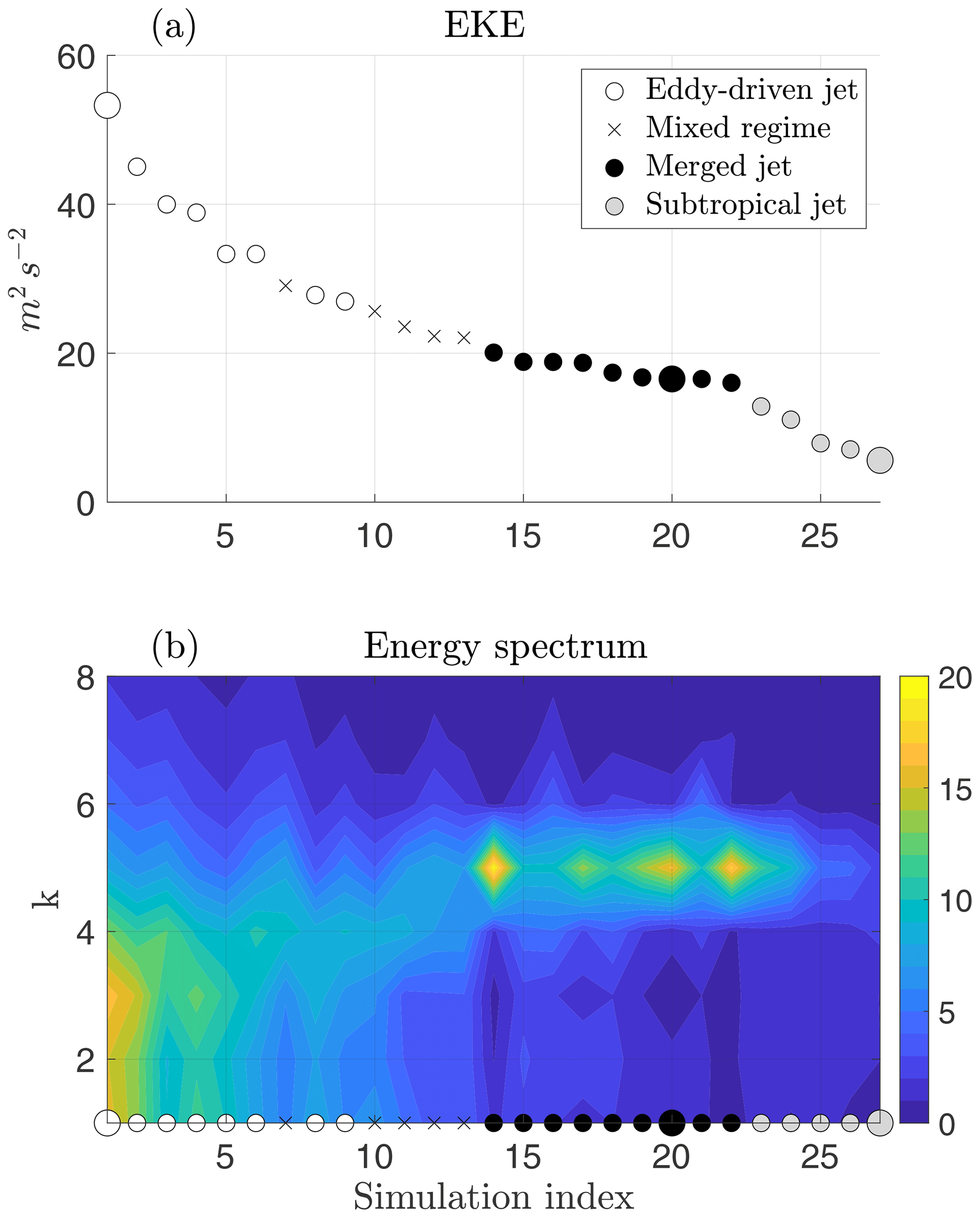
Figure 2(a) Time-mean eddy kinetic energy (EKE) averaged over the model's Southern Hemisphere and (b) the eddy energy spectrum as a function of zonal wavenumber k and simulation index (see Table A1). Units are m2 s−2 for both panels. The markers in both panels indicate the jet regime of each simulation. Open circles, black circles, grey circles, and × indicate the different jet regimes as in the legend. The larger markers indicate the simulations shown in Fig. A1.
2.3 Dynamical systems metrics
The above data are analysed by applying a recently developed approach grounded in dynamical systems theory. This evolved from the findings of Lucarini et al. (2016) and Faranda et al. (2017b), and it allows computing the instantaneous (in time) or local (in phase space) properties of a dynamical system by combining extreme value theory with Poincaré recurrences. A given succession of latitude–longitude maps of an atmospheric variable of interest is interpreted as a long trajectory in a reduced phase space of the atmospheric flow. Each map corresponds to both a specific point in this phase space and a specific time. Instantaneousness in time is therefore equivalent to locality in phase space. Local (instantaneous) properties are then computed for all points (time steps) in our dataset. We specifically compute two metrics, namely the local dimension d and the persistence θ−1.
The local dimension is the local counterpart to the attractor dimension of a dynamical system, the attractor being a geometrical object defined in the phase space hosting all the possible states of the system. The local dimension describes the geometry of the system's trajectory in a small region of the phase space around a state of interest ζ, which in our case could be a latitude–longitude map of barotropic zonal wind from reanalysis data; d may specifically be taken as a proxy for the number of active degrees of freedom of the system about ζ. In other words, it measures how many directions all possible trajectories originating from a certain state in phase space can locally take on the attractor. The persistence θ−1 of a state ζ is a measure of the system's typical residence time in the neighbourhood of ζ: that is, a measure of how long the system persists in states that closely resemble ζ. Both d and θ may be related to a state's intrinsic predictability (Messori et al., 2017; Hochman et al., 2019). Indeed, the attractor dimension is related to error growth and thus predictability. If trajectories are constrained on a low-dimensional manifold, they will be more easily predictable than if they evolve on a high-dimensional phase space with many different directions available (Buschow and Friederichs, 2018). This argument may be extended to d when considering a specific point on the attractor. Thus, a state with a low d will have higher intrinsic predictability than one with a high d. Similarly, one may interpret highly persistent states (high θ−1) as having high intrinsic predictability. Indeed, a high θ−1 implies that a persistence forecast – the simplest possible forecast one can make – will roughly capture the short-term evolution of the state. Forecasting the evolution of highly transient states (low θ−1) will typically require an understanding of the dynamics of the system and thus correspond to lower intrinsic predictability. However, since the degree of predictability is jointly determined by d and θ, specific dynamical regimes such as travelling linear waves may be comparatively predictable and display a low d yet also a low persistence. The fact that both d and θ−1 are local metrics implies that the intrinsic predictability is conceptually different from the predictability inferred from the performance of a numerical weather prediction model. Although the information provided by the two partly overlaps (Scher and Messori, 2018), the former depends on the local geometry of the attractor and on the characteristic timescales of the dynamics in the neighbourhood of the state of interest. On the other hand, the numerical forecasts depend on the specific numerical model used and, for forecasts with a long lead time, on non-local properties of the trajectory.
To estimate the local dimension we leverage the Freitas–Freitas–Todd theorem (Freitas et al., 2010), modified by Lucarini et al. (2012), which characterizes the system's recurrences around the state of interest ζ. The theorem specifically indicates that the cumulative distribution function of suitably defined recurrences of the system about ζ converges to the exponential member of the generalized Pareto distribution (GPD). As detailed in Appendix B, the local dimension may then be estimated directly from the parameters of the GPD. Here, we follow the estimation procedure of Faranda et al. (2019b).
The persistence is instead obtained from the extremal index, which we can interpret as the inverse of the mean cluster size of recurrences about ζ (Moloney et al., 2019). Further details on the estimation of the extremal index and the derivation of θ are provided in Süveges (2007) and Appendix B here. The persistence is bounded in [1,∞] and is in units of the time step of the data. It is therefore essential to use a dataset whose time step is smaller than the typical timescale of the physical processes of interest. An overly long time step would indeed result in all instantaneous states tending to . In line with previous studies, we deem daily data sufficient to capture the salient features of the large-scale jet variability (e.g. Woollings et al., 2010; Madonna et al., 2017).
As a final product of our analysis, one obtains a value of d and θ−1 for every time step and variable in the dataset. Estimating d and θ−1 for real-world data is subject to a number of caveats, as discussed in Appendix B. There are nonetheless both formal and empirical arguments supporting the application of our framework to data that deviate from the theoretical case, and indeed the two dynamical systems metrics have been successfully applied to a variety of climate datasets (e.g. Rodrigues et al., 2018; Scher and Messori, 2019; Hochman et al., 2020; Faranda et al., 2019a, b; Brunetti et al., 2019; De Luca et al., 2020a, b) and more generally to a range of chaotic dynamical systems (Faranda et al., 2020; Pons et al., 2020).
3.1 Model jet regimes
The simple model we adopt can reproduce the three jet regimes: subtropical, merged and eddy-driven. We classify our simulations according to the structure and driving mechanism of the zonal-mean zonal wind and according to the variability and spectral properties of the flow, following Lachmy and Harnik (2016). The subtropical jet is located at the edge of the Hadley cell, displays weak eddy kinetic energy and is maintained by zonal-mean advection of planetary momentum. The merged jet is located inside the Ferrel cell and is maintained mainly by eddy momentum flux convergence. It has a narrow latitudinal structure and a very low latitudinal variability. The eddy-driven jet is also maintained by eddy momentum flux convergence, but it is much wider than the merged jet and displays large fluctuations between a single- and double-jet structure. The characterization of the different flow regimes is further detailed in Appendix A. As the wave energy is increased by decreasing H and/or r (Sect. 2.1), the flow transitions from a subtropical jet regime to a merged jet regime and finally to an eddy-driven jet regime. In Fig. 2a, the different simulations are marked according to the flow regime and sorted by their time-mean EKE. The different spectral properties of the flow in the three regimes are apparent in Fig. 2b. In the merged jet regime the wave spectrum is dominated by a wavenumber 5 mode, whereas in the eddy-driven jet regime the spectrum is much wider and extends to lower wavenumbers. The model further reproduces flows which are a mixture of the eddy-driven and merged jet regimes, meaning that the simulations either vacillate between the two regimes or that the flow displays characteristics of both regimes, depending on the chosen diagnostic variable (crosses in Fig. 2).
3.2 Dynamical characteristics of the model jet regimes
The differences in the time-mean EKE and EKE spectra of the three jet regimes (plus the mixed case) reproduced by the model are related to their different spatio-temporal variabilities (see also Sect. 3.1 and Lachmy and Harnik, 2020). This, in turn, suggests that their dynamical systems characteristics should be different. Wave driving is the dominant mechanism affecting the jet and its variability on a wide range of timescales. A strong EKE and a wide EKE spectrum should favour non-linearities in the flow and allow for a rich set of possible evolutions. The converse holds for weak EKE and a narrow EKE spectrum. We would thus expect the jet stream to be more persistent (smaller θ) and display a lower local dimension d when the EKE is weak and the spectrum is narrower (see also Sect. 5).
We analyse the results for d and θ computed on both barotropic zonal-mean zonal wind and barotropic wave vorticity (Fig. 3). The former (Fig. 3b, d) displays increasing d and θ as the flow transitions from the weak EKE subtropical jet regime (turquoise dots) to the mid-range EKE merged jet (amber dots) and to the strong EKE eddy-driven jet regime (black dots) via the mixed cases (blue dots). Although the spread in d and θ within each simulation is large, the centroids of the different simulations are organized in specific regions in the d–θ phase space according to the corresponding jet regime (Fig. 3d).

Figure 3d–θ diagrams of barotropic wave vorticity (a, c) and barotropic zonal-mean zonal wind (b, d) for all time steps in the model simulations (a, b) as well as centroids for each different simulation. Colours indicate the different jet regimes as in the legend. The turquoise + symbols in (c, d) mark the centroids of the anomalous period in simulation no. 23, which is discussed in Sect. 3.2. Note that higher (lower) θ values correspond to lower (higher) persistence and that the axis ranges differ across the panels.
The picture from the barotropic wave vorticity is more nuanced (Fig. 3a, c). The subtropical jet regime (turquoise dots) typically displays low d and θ, matching the expected weak wave activity and the dominance of thermal maintenance mechanisms. The eddy-driven jet regime (black dots) shows higher d and θ, reflecting the dominant role of eddies and the large meridional excursions in jet location. The merged jet regime (amber dots) and mixed cases (blue dots) display on average a lower d yet a higher θ than the eddy-driven jet regime, although the mixed and eddy-driven cases show substantial overlap in both indicators. A low local dimension coupled with a low persistence is a somewhat unusual combination in terms of both our a priori expectations for the dynamical characteristics of the different jet regimes and the positive correlation between d and θ displayed by most atmospheric variables (e.g. Faranda et al., 2017a, b; Messori et al., 2017). This result may reflect the narrow wave spectrum driving the merged jet regime, leading to a quasi-periodic behaviour in which wave trains with a dominant zonal wavenumber develop and circle the globe with a relatively high phase speed (due to the relatively strong jet) before decaying. The wave field evolution is thus a highly predictable eastward translation with low wind speed variability and a weak meridional meandering of the jet, as reflected in the low local dimension. At the same time, the wave field displays a low persistence due to its relatively fast phase propagation. Consistently, the quasi-linear nature of this regime, in which the waves weaken the jet in place while they decay, results in d and θ values of the barotropic zonal-mean zonal wind which lie between those of the linear subtropical jet regime and the turbulent eddy-driven jet regime (Fig. 3b, d).
A more detailed picture of the evolution of the flow's dynamical characteristics can be obtained by ranking the different simulations by decreasing EKE, which closely mirrors the division between the different jet regimes (Fig. 4). The barotropic wave vorticity displays an increase in θ at the transition between the eddy-driven and merged jet regimes, as well as a large discontinuous decrease in θ at the transition between the merged and subtropical jet regimes around simulation 23 (Fig. 4a). The latter simulation is discussed in further detail below. As discussed above, we interpret the large values of θ in the merged jet regime, which indicate low persistence, as a result of the regime's narrow spectrum with a single dominant propagating wave mode. The barotropic wave vorticity d, on the other hand, shows a decrease as a function of EKE, albeit with significant variability within the individual jet regimes. The highest values of d appear in the most energetic simulations of the eddy-driven jet regime, consistent with their turbulent nature as seen in the wave spectrum (Fig. 2b) and also discussed in Lachmy and Harnik (2016). Both dynamical metrics for the barotropic zonal-mean zonal wind (Fig. 4b, d) display a largely monotonic decrease with increasing simulation index. Again, the transitions between different jet regimes, especially that between the merged and subtropical jet regimes (around simulation 23), emerge as discontinuities. Figure 4 also highlights the range of variability of the dynamical systems metrics within each simulation. Some distributions, such as the local dimension of the subtropical jet regime computed on barotropic wave vorticity (Fig. 4c), are very peaked, indicating homogeneous characteristics of the flow throughout the simulations. Others, such as the eddy-driven regime in the same panel, display a broader peak and a wider range of variability, pointing to the rich dynamical structure of the flow.

Figure 4Distributions of θ (a, b) and d (c, d) values for barotropic wave vorticity (a, c) and barotropic zonal-mean zonal wind (b, d) in the different model runs. The colour scale starts at 100 data points and indicates the number of data points per bin. Bin intervals are 0.05 (θ) or 1 (d). The markers on the x axis indicate the flow regime, as in Fig. 2. The vertical dashed lines indicate the approximate transitions between the different jet regimes. Note that higher (lower) θ values correspond to lower (higher) persistence and that the ordinate ranges differ across panels.
We conclude the overview of the QG model's jet regimes by focusing on simulation no. 23, which serves well to illustrate the sensitivity of the dynamical systems metrics to the instantaneous characteristics of the atmospheric flow. This simulation falls within the subtropical jet regime (Table A1 and Fig. 2a) but displays some anomalous characteristics during a period of approximately 1200 d in the middle of the simulation (Fig. 5c). These are clearly visible in Fig. 4 but also emerge in Fig. 3a as a cloud of turquoise points extending towards high θ values. During this period, the flow is characterized by vacillations between a high-EKE, southerly merged jet regime and a subtropical jet. Unlike the mixed jet simulations, however, this is an isolated occurrence, explaining why the simulation falls into the subtropical jet classification. The dynamical systems metrics enable us to clearly identify this anomalous transition period (red dots in Fig. 5a, b), which covers a separate region of the d–θ space compared to the rest of the simulation. Indeed, the outcropping region in Fig. 3a can be almost exclusively ascribed to the anomalous period (compare Figs. 3a and 5a). The persistence of this period for the barotropic wave vorticity is intermediate between the merged jet and subtropical jet clusters, while the local dimension is close to that of the subtropical jet cluster (turquoise cross in Fig. 3c). The barotropic zonal-mean zonal wind instead displays anomalously low local dimension and persistence, with the former being much lower than even those of the linear subtropical jet regime (turquoise cross in Fig. 3d). Thus, in simulation no. 23 the dynamical systems metrics reflect the transition of the jet to a state with peculiar dynamical properties.
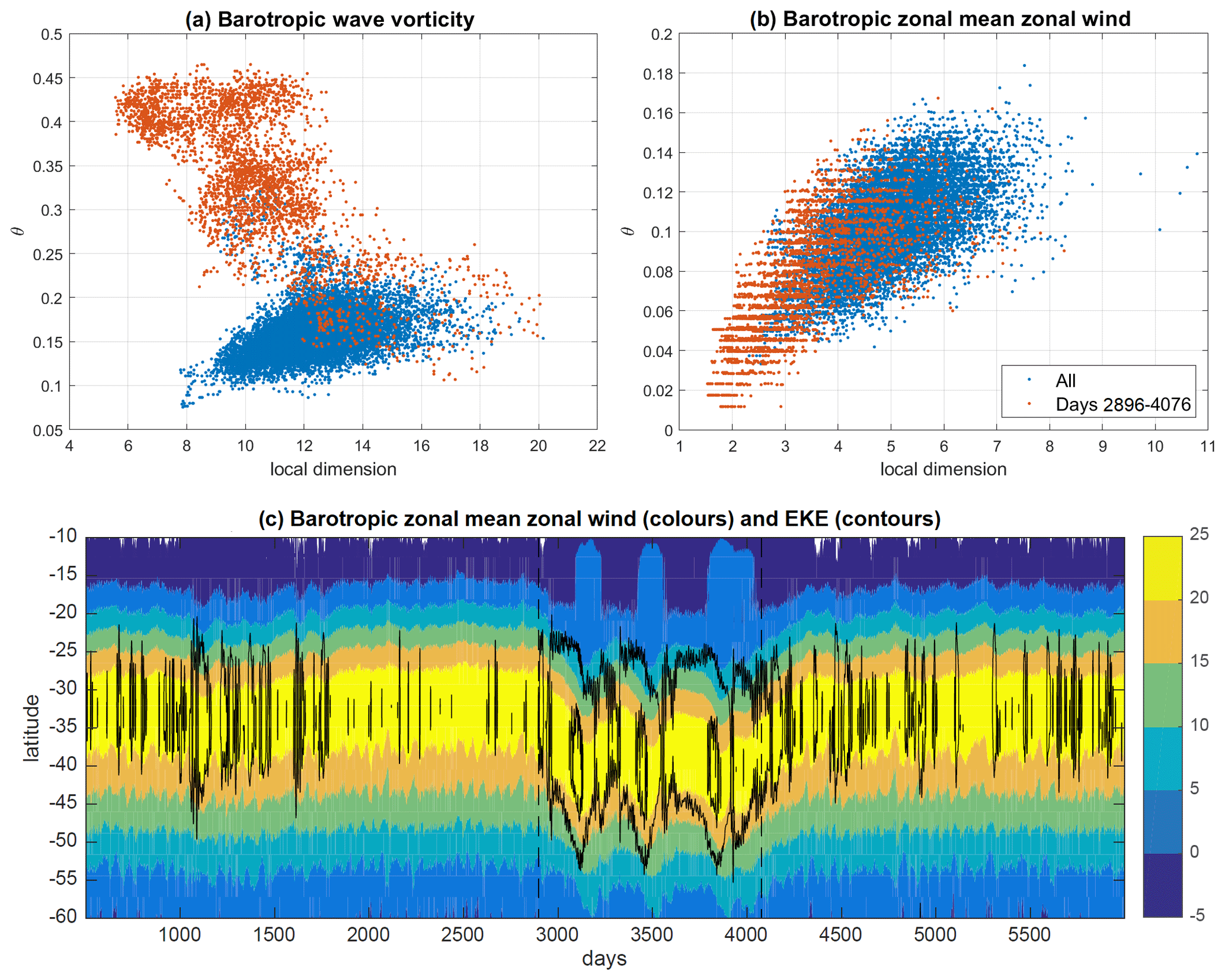
Figure 5The d–θ diagrams of barotropic wave vorticity (a) and barotropic zonal-mean zonal wind (b) for all time steps in simulation no. 23 (see Table A1). (c) Latitude–time diagram of barotropic zonal-mean zonal wind (m s−1, colours) and eddy kinetic energy (EKE, m2 s−2, contours) for the same simulation. The red dots in (a, b) correspond to days 2896–4076 in the simulation. These were chosen based on a visual inspection of panel (c) and are marked by the two vertical dashed lines. Contours in (c) are at 60 and 120 m2 s−2. Note that the axis ranges differ between panels (a) and (b).
As discussed in the Introduction, purely thermally driven or eddy-driven jets are largely theoretical constructs. Moreover, for a given region and season, the jet typically displays large intraseasonal variability and a range of different flow characteristics (e.g. Bals-Elsholz et al., 2001; Nakamura and Shimpo, 2004; Woollings et al., 2010; Harnik et al., 2014; Messori and Caballero, 2015; Madonna et al., 2017). On this basis, we expect the jets observed in the real atmosphere to blend the dynamical characteristics of the different jet regimes reproduced in the QG model.
To verify whether our dynamical systems approach can distinguish between different jet regimes in the real atmosphere, we therefore take a slightly different angle from that used in our idealized model, although the analysis tools are identical to those used above. We compute d and θ on barotropic zonal wind (see Sect. 2.2) but consider flow anomalies associated with concurrent low or high values of d and θ. We define these as values beyond the 10th or 90th percentiles of the respective distributions. The choice of joint high or low percentiles is dictated by the fact that the different jet regimes in Fig. 3b and d align chiefly along a d–θ diagonal. The analysis focuses on austral winter (JJA) over the Pacific domain shown in Fig. 1, which is chosen because it displays a variety of jet regimes. During the austral winter, the signature of the subtropical – and predominantly thermally driven – jet is evident at upper levels around 30∘ S, while that of the polar – and predominantly eddy-driven – jet emerges most clearly at lower levels around 60∘ S (Fig. 1). Periods when these flows are well-separated alternate with periods dominated by a single nearly barotropic flow, akin to a merged jet.
When both d and θ are anomalously low, the upper-level zonal wind (300 hPa) displays a clear maximum around 30∘ S, coincident with the climatological location of the subtropical jet and characterized by above-average speeds (Fig. 6a). The signature of this jet extends to the lower troposphere, where a low-level (850 hPa) zonal wind maximum located slightly poleward of the 300 hPa maximum is clearly visible on the same days, especially in the eastern part of the domain (Fig. 6c). This inference is confirmed by analysing the vertical cross section of the zonal flow, which evidences a poleward displacement of the location of the zonal wind maximum at 850 hPa compared to 300 hPa (Fig. 6e). The EKE shows widespread negative anomalies across the central and southern portions of the domain and localized positive anomalies at 300 hPa matching the latitude of the jet (Fig. 7a, c). We interpret the above characteristics as the signature of a merged jet.
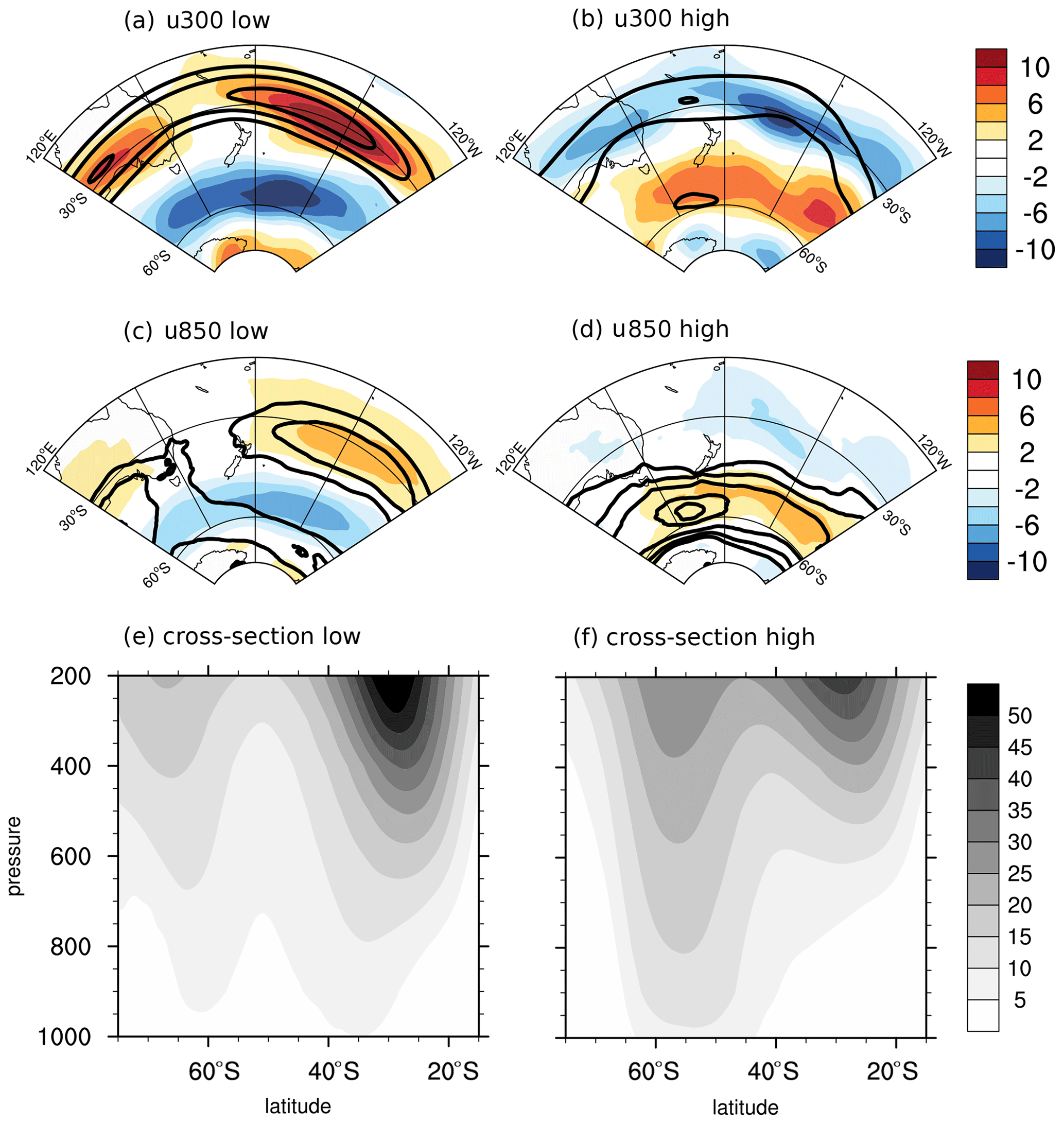
Figure 6JJA zonal wind composites (m s−1) at 300 hPa (a, b) and 850 hPa (c, d) as well as zonal-mean zonal wind composite cross sections over the South Pacific domain (120 ∘ W–120 ∘ E). Separate composites are shown for days displaying low (a, c, e) and high (b, d, f) values of d and θ. See text for details. In (a)–(d), colours show deviations from the climatology, while contours show absolute values. Contours are every 10 m s−1 starting from 30 m s−1 in (a) (b) and every 3 m s−1 starting from 6 m s−1 in (c, d).

Figure 7JJA EKE composites (m2 s−2) at 300 hPa (a, b) and 850 hPa (c, d) for days displaying low (a, c) and high (b, d) values of d and θ. See text for details. Colours show deviations from the climatology, while contours show absolute values. Contours are every 20 m2 s−2 starting from 40 m2 s−2 in (a, b) and every 5 m2 s−2 starting from 10 m2 s−2 in (c, d).
When both d and θ are anomalously high, the upper-level zonal flow evidences two maxima: a weaker-than-climatology jet around 30 ∘S and an anomalous secondary maximum at around 55∘ S, associated with large positive zonal wind speed anomalies (Fig. 6b). At low levels, there is a single jet located just to the north of 60 ∘S associated with large positive zonal flow anomalies (Fig. 6d). The southern jet therefore has a more pronounced barotropic structure than its northern counterpart, as also seen in the vertical cross section of the zonal flow (Fig. 6f). The EKE anomalies are predominantly positive across the central and southern portions of the domain (Fig. 7b, d). The above points to a primarily eddy-driven jet in the south and a primarily thermally driven jet further north, in agreement with the theoretical framework of Lee and Kim (2003) and Son and Lee (2005). It also suggests that the persistence of the double-jet configuration, with a strong eddy-driven jet, is lower (high θ) than that of the single merged jet (low θ).
We have analysed different jet regimes in a set of idealized simulations with a QG model and reanalysis data. The QG model reproduces the full range of theoretically derived jet regimes (e.g. Lee and Kim, 2003; Son and Lee, 2005; Lachmy and Harnik, 2016). These are an eddy-driven jet, a merged jet and a subtropical jet. It additionally reproduces transition states between a merged and eddy-driven jet, which we term mixed jets. Pure eddy-driven or thermally driven jets are largely theoretical constructs, and in the real atmosphere the separation between them is often blurred. Nonetheless, it is possible to identify primarily eddy-driven, primarily thermally driven and merged jets (e.g. Koch et al., 2006; Eichelberger and Hartmann, 2007; Li and Wettstein, 2012). The South Pacific sector is of particular interest in this context, since it is a region where the three main jet regimes may be observed at the same longitude (e.g. Bals-Elsholz et al., 2001; Nakamura and Shimpo, 2004).
Relating the different jet regimes identified in idealized models to those identified in reanalysis data is far from immediate. Here, we have proposed an analysis approach which may be applied to both datasets and which provides a direct link between the characteristics of the jets in the QG model and those seen in the ERA-Interim dataset. Such an approach is grounded in dynamical systems theory and is based on two metrics, d and θ, which characterize the instantaneous (local in phase space) dynamical characteristics of the jet. The local dimension d is a proxy for the number of active degrees of freedom of the system. The persistence θ−1 is a measure of the typical residence time of the system in the neighbourhood of a given state. Their computation arises from an analysis of recurrences of the system, and both may be related to the concept of predictability. Indeed, one may expect low d, high θ−1 states to be more predictable than high d, low θ−1 situations (see Sect. 2.3). This interpretation is confirmed by ongoing work by some of the authors, which finds a direct link between precipitation forecast skills at single stations in France and the values of d and θ computed for 500 hPa geopotential height fields in the preceding days. Unlike conventional approaches which diagnose the driving mechanisms of the jet in terms of complex physical processes, such as convection or eddy momentum flux convergence, the dynamical systems metrics allow us to delineate the dynamical properties of the jet uniquely from computing d and θ on the wind itself. Differently from previous studies using this approach, here we have thus attempted to link the dynamical systems metrics directly to the physical mechanisms of jet maintenance. As a caveat, we note that the absolute values of these metrics should be interpreted in a relative sense within each dataset they are computed on and that direct comparison of their magnitudes across datasets should be treated with caution. From a theoretical standpoint, there are cogent arguments supporting the use of recurrences of observables of a system to investigate the properties of the system's underlying phase space, even though all the variables defining said phase space cannot be considered (e.g. Faranda et al., 2017a, c; Barros et al., 2019). This makes our analysis affordable in terms of computational and data requirements – indeed, d and θ for a single variable from a reanalysis dataset may be computed by a modern laptop computer in a matter of hours – and versatile in terms of applicability to very different datasets (see Rodrigues et al., 2018; Faranda et al., 2019c; Pons et al., 2020). Moreover, d and θ do not require prior knowledge of the exact location of the jet.
In the QG model, d and θ allow us to characterize the different jet regimes. Specifically, when computed on barotropic zonal-mean zonal wind they highlight the eddy-driven jet as being a low-persistence, high-dimensional regime, the subtropical jet as being a high-persistence, low-dimensional regime and the merged jet as having intermediate dynamical characteristics. This reflects the wide wave spectrum and large latitudinal fluctuations in the eddy-driven jet versus the lower latitudinal variability of the subtropical jet. Indeed, in the former regime the energetic wave activity, the comparatively broad wave spectrum and the range of wave phase speeds offer a variety of different temporal evolutions of the atmospheric flow. In the latter regime, the flow instead displays a weak eddy kinetic energy and a narrow wave spectrum, with a correspondingly narrow range of wave phase speeds and meridional excursions. Moreover, the typically similar wavelength and phase speed of the waves implies that the temporal evolution of the atmospheric flow is relatively repetitive. Lachmy and Harnik (2016, 2020) further analysed the EKE budgets of different jet regimes in terms of the contributions by linear versus eddy–eddy interactions and found that the degree of linearity of the dynamics changes. The subtropical regime is comparatively linear, the merged regime's variability is dominated by wave-mean flow interactions, and the eddy-driven regime is non-linear with a turbulent upscale energy cascade. Intuitively, we expect the predictability of the flow to decrease and the jet structure to vary more strongly in time as the flow becomes more non-linear. The dynamical systems metrics thus reflect the theoretical expectations of the role of increased EKE in decreasing predictability (Leith, 1971). In contrast to the jet variability, the model's jet speed (Fig. A1) is not related to the degree of non-linearity of the flow. Because of this, changes in jet speed may not map directly onto differences in d and θ.
A natural question to ask is whether d and θ also reflect variability within the individual simulations in the QG model. A preliminary analysis of the barotropic zonal-mean zonal wind for one of the simulations classified as an eddy-driven regime (simulation no. 2; see Table A1) shows that, when d and θ are very low, the jet has large variability (red line in Fig. A2c) and a narrow profile reminiscent of the merged jet regime (compare the red line in Fig. A2b with the amber line in Fig. A1). This may be contrasted with the average jet structure for this simulation, which is quite wide with an inflection suggestive of a separation between the eddy-driven and subtropical jets (grey line, Fig. A2b). During low d and θ time steps, the jet also displays a much sharper EKE spectrum (not shown) and a more equatorward lower-level jet (red line, Fig. A2d) than climatology. On the other hand, when d and θ are anomalously large, the lower-level jet is slightly more poleward and intense than usual (compare the grey and blue lines in Fig. A2d), and the spread in jet profiles is unusually low (blue line in Fig. A2c). The resemblance between low d and θ time steps in an eddy-driven jet simulation and the flow characteristics seen in merged jet regime simulations is consistent with inter-regime differences in the two dynamical systems indicators. Indeed, simulations classified as merged jet regimes generally display lower d and θ values than simulations within the eddy-driven regime (Fig. 3b). Lachmy and Harnik (2020) also found that the temporal variability of the eddy-driven jet includes a merged-jet-like state.
The results for reanalysis data largely mirror those found for the idealized simulations. Focusing on the Pacific sector of the Southern Ocean, d and θ computed on the barotropic zonal wind again discriminate between different jet regimes. Specifically, high d, high θ days display both a thermally driven subtropical jet and a strong eddy-driven polar-front jet, while low d, low θ days display a merged jet. A key difference from the results in the QG model is that, in the reanalysis data, the South Pacific sector we consider does not display a purely thermally driven nor a purely eddy-driven jet. Indeed, both jet regimes co-occur at different latitudes during winter. The upper-level jet is stronger in the single-jet merged configuration compared to the double-jet configuration (compare Fig. 6a and b), consistent with the idealized results of Son and Lee (2005).
The distinction between eddy-driven, merged and subtropical jets also applies to the Northern Hemisphere (NH) (e.g. Eichelberger and Hartmann, 2007; Li and Wettstein, 2012). Moreover, within the same ocean basin the jet can transition between different regimes. Therefore, there is no a priori reason that our analysis framework should not be applicable to NH dynamics. For example, in the North Atlantic sector one may expect the climatological co-existence of an eddy-driven jet and a subtropical jet to correspond to high d and θ states and the rarer merged jet conditions (e.g. Harnik et al., 2014; Madonna et al., 2019) to correspond to lower d and θ values. However, zonal asymmetries linked to land–sea contrast and orography are more prominent than in the SH (e.g. Brayshaw et al., 2009). The observed separation in d–θ space between the different jet regimes may be affected by this, although it is not straightforward to infer exactly how without conducting a full analysis. Here, our intention is not to provide a systematic analysis of atmospheric jet characteristics in different geographical regions. Rather, by building upon both idealized simulations and reanalysis data, we illustrate the potential of dynamical systems indicators to diagnose jet regimes in a conceptually intuitive fashion.
The two-layer QG model, described in Sect. 2.1, solves the equations outlined below for the barotropic (vertical mean) and baroclinic (half the difference between the upper and lower layers) components of the zonal-mean zonal momentum equation,
and the diagnostic equation for ,
where , and μ≡sin ϕ. The variables u and v are the zonal and meridional winds, respectively, and ϕ is the latitude. Subscripts M and T denote the barotropic and baroclinic components, respectively. Overbars denote zonal means and primes denote deviations from the zonal mean. The constants Ω, a, τf, τr and ν are the Earth's rotation rate and radius, the surface friction timescale, the radiative damping timescale, and the numerical diffusion coefficient, respectively. The non-dimensional parameter ϵ is defined as , where N is the Brunt–Väisälä frequency.
Table A1The model simulations sorted by the EKE in descending order. The parameters H and r are the layer thickness in kilometres and the dimensionless wave-damping parameter, respectively. The simulations are categorized according to their flow regime (see text). Simulations with mixed properties of the merged jet and eddy-driven jet regimes are denoted as a “mixed regime”.
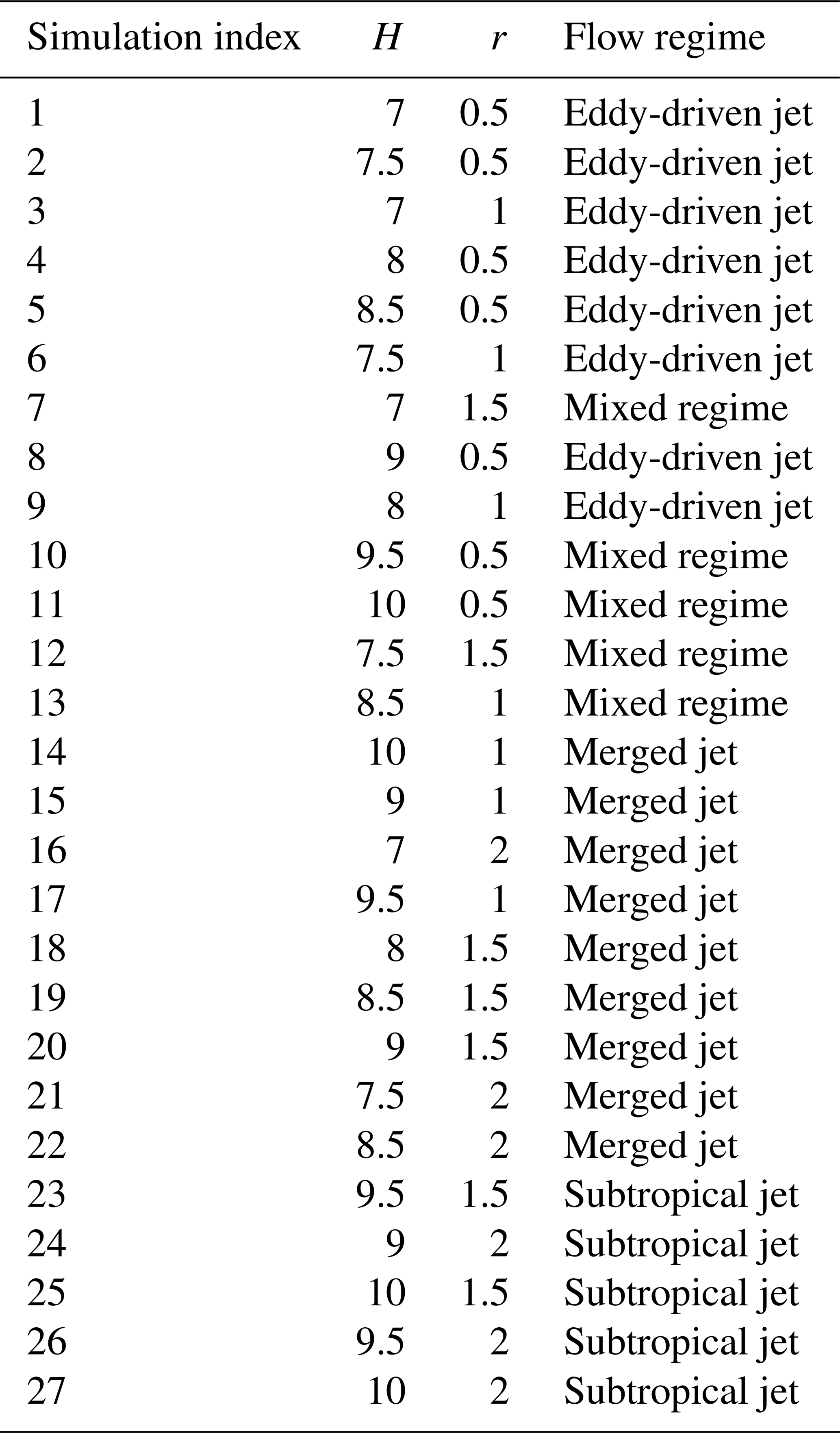
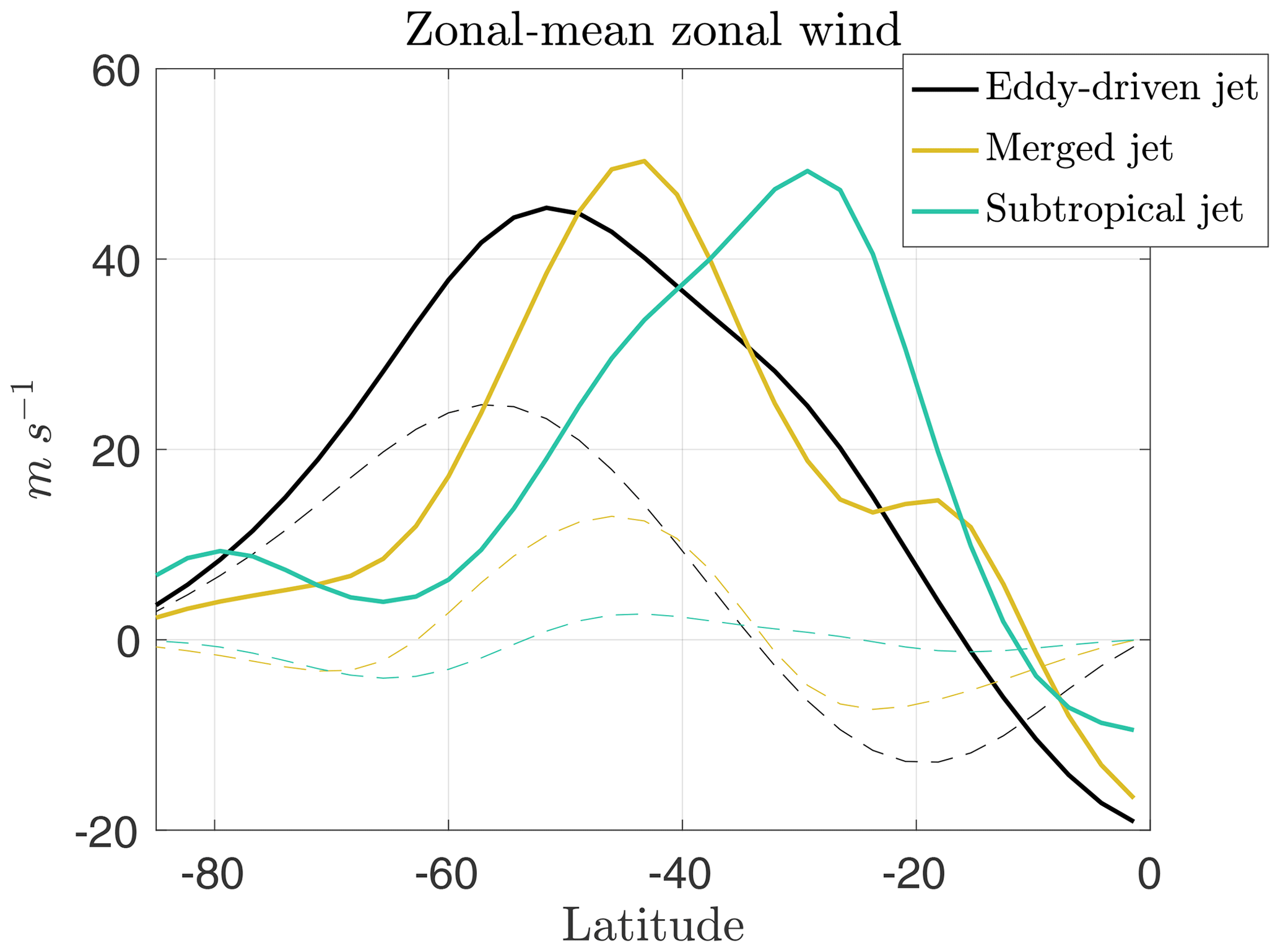
Figure A1Zonal-mean zonal wind (m s−1) in the upper (, thick solid lines) and lower (, thin dashed lines) layers of the two-layer QG model for simulation number 1 from the eddy-driven jet regime, simulation number 20 from the merged jet regime and simulation number 27 from the subtropical jet regime. Colours indicate the different jet regimes as in the legend. See Table A1 for the parameters of the simulations.
The barotropic and baroclinic components of the wave potential vorticity (PV) equation are as follows.
Here, λ is the longitude in radians; q and ψ are the PV and stream function, respectively, which satisfy the following relation:
The components of the mean PV gradient, and , which appear in Eqs. (A3a) and (A3b), are
The model includes several parameters which were fixed for all the experiments in this study. The surface friction and radiative relaxation timescales are τf=3.9 d and τr=11.6 d, respectively. The radiative equilibrium profile of the thermal wind, , is the following profile smoothed by a running average filter,
where (uT)0=15 and . This profile causes the Hadley cell's ascending branch to be concentrated around ϕ0 and is meant to simulate winter conditions for the SH of the model. The diffusion coefficients for the mean flow and the waves are m4 s−1 and m4 s−1, respectively. These parameter choices follow Lachmy and Harnik (2016).
The flow regimes in the model are characterized according to the structure of the zonal-mean flow and the properties of the wave spectrum (Lachmy and Harnik, 2016). The diagnosed regimes for each of the simulations are listed in Table A1. The different structures of the zonal-mean zonal wind are shown in Fig. A1 for three simulations, one from each regime. The upper-layer zonal wind (thick solid lines) represents the upper-tropospheric jet stream. The lower-layer zonal wind (thin dashed lines) indicates the structure of the mean meridional circulation, since according to the zonal-mean momentum balance, it is positive in the Ferrel cell and negative in the Hadley and polar cells (Lachmy and Harnik, 2014). We identify the mechanism maintaining the jet according to the relative location of the upper- and lower-layer zonal wind maxima. The subtropical jet (turquoise lines) is thermally driven, since its upper-layer zonal wind maximum is at the Hadley cell edge, where the lower-layer zonal wind is zero. The merged jet (amber lines) and eddy-driven jet (black lines) are located inside the Ferrel cell, where the lower-layer zonal wind is maximal, indicating that they are driven by eddy momentum flux convergence. In the merged jet regime the jet inside the Ferrel cell is collocated with the maximum vertical shear of the zonal wind, which indicates that it represents a merging of the subtropical and eddy-driven jets. In the eddy-driven jet regime the two maxima are separated, indicating that the upper-layer zonal wind maximum represents a purely eddy-driven jet (Lachmy and Harnik, 2016).

Figure A2A d–θ diagram of barotropic zonal-mean zonal wind (a) for simulation no. 2 (see Table A1) and composites over time steps with low (<10th) and high (>90th) percentiles of both d and θ, upper-level (b) and lower-level (d) zonal-mean zonal wind (m s−1), and (c) barotropic zonal-mean zonal wind standard deviation. The vertical bars in (b) and (d) show the standard deviations of the relevant composites at a given latitude. The red and blue dots (a) and lines and bars (b–d) correspond to low and high d–θ time steps, respectively, while grey marks all other times (a) or the simulation's climatology (b–d). The numbers in parentheses in (a) show the sample size of the each composite. Thick lines in (b) and (d) denote latitudes at which the high or low d and θ composites are significantly different from the simulation's climatology at the 95 % confidence level based on a two-sided Student's t test.
The attractor of a dynamical system is a geometric object defined in the space hosting all the possible states of the system (phase space). For each point ζ on the attractor, two dynamical indicators can be computed to characterize the recurrence properties of ζ. The local dimension d indicates the number of degrees of freedom active locally around ζ; the persistence θ−1 is a measure of the mean residence time of the system around ζ (Faranda et al., 2017b). To determine d, a key observation is the connection between extreme value theory and the Poincaré recurrences of a state ζ in a chaotic dynamical system. We consider long trajectories of a dynamical system – in our case successions of daily atmospheric latitude–longitude maps – to be a sequence of states on the attractor. This equates to approximating the attractor with its Sinai–Ruelle–Bowen (SRB) measure (Young, 2002) and establishes a connection between the attractor and the histogram of visits in phase space. For a given point ζ in phase space (e.g. a given atmospheric latitude–longitude map), one may then compute the probability that the system returns within a ball of radius ϵ centred on ζ, which follows an extreme value distribution. Indeed, the Freitas–Freitas–Todd theorem (Freitas et al., 2010), modified by Lucarini et al. (2012), states that logarithmic returns,
yield a probability distribution such that
This is the exponential member of the generalized Pareto distribution family, with and s a high threshold associated with a quantile q of the series g(x(t),ζ). Requiring that the orbit falls within a ball of radius ϵ around the point ζ is equivalent to asking that the series g(x(t),ζ) exceeds the threshold s; therefore, the ball radius ϵ is simply e−s(q). The parameters μ and σ, namely the location and the scale parameters of the distribution, depend on the point ζ in phase space; μ(ζ) corresponds to the threshold s(q), while the local dimension d(ζ) is obtained as .
When x(t) contains all the variables of the system, the estimation of d based on extreme value theory has a number of advantages over traditional methods (e.g. the box counting algorithm; Liebovitch and Toth, 1989; Sarkar and Chaudhuri, 1994). First, it does not require an estimate of the volume of different sets in scale space: the selection of s(q) based on the quantile provides a selection of different scales s, which depend on the recurrence rate around the point ζ. Moreover, it does not require the a priori selection of the maximum embedding dimension, as the observable g is always a univariate time series.
The persistence of the state ζ is measured via the extremal index , a dimensionless parameter which measures the inverse of cluster lengths for consecutive exceedances of s or, in other terms, recurrences. From this we extract , where Δt is the time step of the data. θ(ζ) is therefore the inverse of the average residence time of trajectories around ζ and is in units of frequency (in this study d−1). If ζ is a fixed point of the attractor, θ(ζ)=0. For a trajectory that leaves the neighbourhood of ζ at the next time iteration, θ=1. To estimate ϑ, we adopt the Süveges maximum likelihood estimator (Süveges, 2007). This approximates the value of ϑ for processes with asymptotically independent inter-cluster times, with the threshold s and the length of the time series as asymptotes. The estimator performs a first guess of the value of ϑ by using the exponential nature of the inter-cluster times. Then, a second estimate is given by extending the definition of clusters to include sequences of exceedances interrupted by short “gaps” which are not distributed exponentially and may therefore be viewed as single clusters. The first estimate provides an upper bound on ϑ and the second estimate a lower bound. The algorithm is then iterated until it reaches a stable point. Heuristically, clusters should be much shorter than inter-cluster times. The other assumptions underlying this calculation largely match those made to compute d, as discussed below. For ease of computation, we prefer the Süveges estimator to the exact formulas provided by Caby et al. (2020), which are anyways conceived for periodic points seldom encountered in natural systems. For further details on the extremal index, we refer the reader to Moloney et al. (2019) and Caby et al. (2020).
The above framework, in particular the Freitas–Freitas–Todd theorem (Freitas et al., 2010), holds for stationary axiom-A systems in the limit of infinite time series. In this respect, climate data, specifically reanalysis data, pose a number of challenges. The dynamics of the system are non-axiom-A and non-stationary, which means that different areas of the attractor do not necessarily share the same properties; data assimilation introduces what is effectively a stochastic component, and the available historical series are all but infinite. A formal justification of the applicability of the dynamical systems metrics to natural data is given in Caby et al. (2020). The authors link the deviations of local dimensions from the asymptotic values of the attractor dimension to singular points of the dynamics. The latter's influence at a finite time modifies the behaviour of their extended neighbourhood, producing large deviations of dynamical quantities, such as local dimensions and persistence. This points to the applicability of the extreme value framework to real-world data. Empirical tests support this conclusion, and indeed Buschow and Friederichs (2018) have shown that d successfully reflects the dynamical characteristics of the atmosphere even when applied to datasets that deviate from the theoretical case and when universal convergence to the exponential member of the GPD is not achieved.
The code to compute the dynamical systems indicators used in this study is made freely available through the cloud storage of the Centre National de la Recherche Scientifique (CNRS) under a CC BY-NC 3.0 license: https://mycore.core-cloud.net/index.php/s/pLJw5XSYhe2ZmnZ (Faranda, 2021).
ERA-Interim reanalysis data can be downloaded from https://apps.ecmwf.int/datasets/data/interim-full-daily/ (ECMWF, 2020). The two-layer QG model data used to compute the dynamical systems indicators can be downloaded from https://www.tau.ac.il/~harnik/ModelsData/ModelsData.html (Lachmy and Harnik, 2021).
GM and NH designed the study. NH and OL performed the analysis of the jet regimes on model data. DF performed the dynamical systems analysis on model data. EM and GM performed the analysis on ERA-Interim data. All authors contributed to drafting the paper. GM coordinated the revision of the paper.
The authors declare that they have no competing interests
All authors would like to thank the three anonymous reviewers for their pertinent and detailed comments as well as the editor for overseeing a very constructive review process.
Gabriele Messori has been partly supported by the Swedish Research Council Vetenskapsrådet (grant no. 2016-03724), and Nili Harnik has been supported by the Israeli Science Foundation (grant no. 1685/17).
The article processing charges for this open-access
publication were covered by Stockholm University.
This paper was edited by Rui A. P. Perdigão and reviewed by three anonymous referees.
Bals-Elsholz, T. M., Atallah, E. H., Bosart, L. F., Wasula, T. A., Cempa, M. J., and Lupo, A. R.: The wintertime Southern Hemisphere split jet: Structure, variability, and evolution, J. climate, 14, 4191–4215, 2001. a, b, c, d
Barros, V., Liao, L., and Rousseau, J.: On the shortest distance between orbits and the longest common substring problem, Adv. Math., 344, 311–339, 2019. a
Brayshaw, D. J., Hoskins, B., and Blackburn, M.: The basic ingredients of the North Atlantic storm track. Part I: Land–sea contrast and orography, J. Atmos. Sci., 66, 2539–2558, 2009. a
Brunetti, M., Kasparian, J., and Vérard, C.: Co-existing climate attractors in a coupled aquaplanet, Clim. Dyn., 53, 6293–6308, 2019. a
Buschow, S. and Friederichs, P.: Local dimension and recurrent circulation patterns in long-term climate simulations, Chaos, 28, 083124, https://doi.org/10.1063/1.5031094, 2018. a, b
Caby, T., Faranda, D., Vaienti, S., and Yiou, P.: Extreme value distributions of observation recurrences, Nonlinearity, 34, 118, https://doi.org/10.1088/1361-6544/abaff1, 2020. a, b
Caby, T., Faranda, D., Vaienti, S., and Yiou, P.: Extreme value distributions of observation recurrences, arXiv preprint, arXiv:2002.10873, 2020. a
De Luca, P., Messori, G., Faranda, D., Ward, P. J., and Coumou, D.: Compound warm–dry and cold–wet events over the Mediterranean, Earth Syst. Dynam., 11, 793–805, https://doi.org/10.5194/esd-11-793-2020, 2020a. a
De Luca, P., Messori, G., Pons, F. M., and Faranda, D.: Dynamical systems theory sheds new light on compound climate extremes in Europe and Eastern North America, Q. J. Roy. Meteor. Soc., 2020b. a
Dee, D. P., Uppala, S. M., Simmons, A. J., Berrisford,P., Poli, P., Kobayashi, S., Andrae, U., Balmaseda, M. A., Balsamo, G., Bauer, P., Bechtold, P., Beljaars, A. C. M., van de Berg, L., Bidlot, J., Bormann, N., Delsol, C., Dragani, R., Fuentes, M., Geer, A. J., Haimberger, L., Healy, S. B., Hersbach, H., Hólm, E. V., Isaksen, L., Kållberg, P., Köhler, M., Matricardi, M., McNally, A. P., Monge‐Sanz, B. M., Morcrette, J.-J., Park, B.‐K., Peubey, C., de Rosnay, P., Tavolato, C., Thépaut, J.-N., and Vitart, F.: The ERA-Interim reanalysis: Configuration and performance of the data assimilation system, Q. J. Roy. Meteor. Soc., 137, 553–597, 2011. a
ECMWF: ERA-Interim data, available at: https://apps.ecmwf.int/datasets/data/interim-full-daily/levtype=sfc/, last access: 7 July 2020. a
Eichelberger, S. J. and Hartmann, D. L.: Zonal jet structure and the leading mode of variability, J. Climate, 20, 5149–5163, 2007. a, b, c
Faranda, D.: Dyn_Sys_Analysis_Matlab_Package, available at: https://mycore.core-cloud.net/index.php/s/pLJw5XSYhe2ZmnZ, last access: 10 February 2021. a
Faranda, D., Messori, G., Alvarez-Castro, M. C., and Yiou, P.: Dynamical properties and extremes of Northern Hemisphere climate fields over the past 60 years, Nonlin. Processes Geophys., 24, 713–725, https://doi.org/10.5194/npg-24-713-2017, 2017a. a, b
Faranda, D., Messori, G., and Yiou, P.: Dynamical proxies of North Atlantic predictability and extremes, Sci. Rep.-UK, 7, 41278, https://doi.org/10.1038/srep41278, 2017b. a, b, c, d
Faranda, D., Sato, Y., Saint-Michel, B., Wiertel, C., Padilla, V., Dubrulle, B., and Daviaud, F.: Stochastic chaos in a turbulent swirling flow, Phys. Rev. Lett., 119, 014502, https://doi.org/10.1038/srep41278, 2017c. a
Faranda, D., Alvarez-Castro, M. C., Messori, G., Rodrigues, D., and Yiou, P.: The hammam effect or how a warm ocean enhances large scale atmospheric predictability, Nat. Commun., 10, 1316, https://doi.org/10.1038/s41467-019-09305-8, 2019a. a
Faranda, D., Messori, G., and Vannitsem, S.: Attractor dimension of time-averaged climate observables: insights from a low-order ocean-atmosphere model, Tellus A, 71, 1–11, 2019b. a, b
Faranda, D., Sato, Y., Messori, G., Moloney, N. R., and Yiou, P.: Minimal dynamical systems model of the Northern Hemisphere jet stream via embedding of climate data, Earth Syst. Dynam., 10, 555–567, https://doi.org/10.5194/esd-10-555-2019, 2019c. a, b
Faranda, D., Messori, G., and Yiou, P.: Diagnosing concurrent drivers of weather extremes: application to warm and cold days in North America, Clim. Dyn., 54, 2187–2201, 2020. a
Freitas, A. C. M., Freitas, J. M., and Todd, M.: Hitting time statistics and extreme value theory, Probab. Theory Rel., 147, 675–710, 2010. a, b, c
Gallego, D., Ribera, P., Garcia-Herrera, R., Hernandez, E., and Gimeno, L.: A new look for the Southern Hemisphere jet stream, Clim. Dyn., 24, 607–621, 2005. a
Harnik, N., Galanti, E., Martius, O., and Adam, O.: The anomalous merging of the African and North Atlantic jet streams during the Northern Hemisphere winter of 2010, J. Climate, 27, 7319–7334, 2014. a, b, c
Heaviside, C. and Czaja, A.: Deconstructing the Hadley cell heat transport, Q. J. Roy. Meteor. Soc., 139, 2181–2189, 2013. a
Held, I. M.: Momentum transport by quasi-geostrophic eddies, J. Atmos. Sci., 32, 1494–1497, 1975. a
Held, I. M. and Hou, A. Y.: Nonlinear axially symmetric circulations in a nearly inviscid atmosphere, J. Atmos. Sci., 37, 515–533, 1980. a, b, c
Held, I. M. and Larichev, V. D.: A scaling theory for horizontally homogeneous, baroclinically unstable flow on a beta plane, J. Atmos. Sci., 53, 946–952, 1996. a
Hochman, A., Alpert, P., Harpaz, T., Saaroni, H., and Messori, G.: A new dynamical systems perspective on atmospheric predictability: Eastern Mediterranean weather regimes as a case study, Sci. Adv., 5, eaau0936, https://doi.org/10.1126/sciadv.aau0936, 2019. a
Hochman, A., Alpert, P., Kunin, P., Rostkier-Edelstein, D., Harpaz, T., Saaroni, H., and Messori, G.: The dynamics of cyclones in the twentyfirst century: the Eastern Mediterranean as an example, Clim. Dynam., 54, 561–574, https://doi.org/10.1007/s00382-019-05017-3, 2020. a
Hoskins, B. J., James, I. N., and White, G. H.: The shape, propagation and mean-flow interaction of large-scale weather systems, J. Atmos. Sci., 40, 1595–1612, 1983. a
Inatsu, M. and Hoskins, B. J.: The zonal asymmetry of the Southern Hemisphere winter storm track, J. Climate, 17, 4882–4892, 2004. a
Koch, P., Wernli, H., and Davies, H. C.: An event-based jet-stream climatology and typology, Int. J. Climatol., 26, 283–301, 2006. a, b, c, d
Lachmy, O. and Harnik, N.: The transition to a subtropical jet regime and its maintenance, J. Atmos. Sci., 71, 1389–1409, 2014. a, b, c
Lachmy, O. and Harnik, N.: Wave and jet maintenance in different flow regimes, J. Atmos. Sci., 73, 2465–2484, 2016. a, b, c, d, e, f, g, h, i, j, k, l, m
Lachmy, O. and Harnik, N.: Tropospheric jet variability in different flow regimes, Q. J. Roy. Meteor. Soc., 146, 327–347, 2020. a, b, c, d, e
Lachmy, O. and Harnik, N. Two-layer QG model data, avalable at: https://www.tau.ac.il/~harnik/ModelsData/ModelsData.html, last access: 18 February 2021. a
Lee, S.: Maintenance of multiple jets in a baroclinic flow, J. Atmos. Sci., 54, 1726–1738, 1997. a
Lee, S. and Kim, H.-k.: The dynamical relationship between subtropical and eddy-driven jets, J. Atmos. Sci., 60, 1490–1503, 2003. a, b
Leith, C.: Atmospheric predictability and two-dimensional turbulence, J. Atmos. Sci., 28, 145–161, 1971. a
Li, C. and Wettstein, J. J.: Thermally driven and eddy-driven jet variability in reanalysis, Journal of Climate, 25, 1587–1596, 2012. a, b, c
Liebovitch, L. S. and Toth, T.: A fast algorithm to determine fractal dimensions by box counting, Phys. Lett. A, 141, 386–390, 1989. a
Lucarini, V., Faranda, D., and Wouters, J.: Universal behaviour of extreme value statistics for selected observables of dynamical systems, J. Stat. Phys., 147, 63–73, 2012. a, b
Lucarini, V., Faranda, D., de Freitas, J. M. M., Holland, M., Kuna, T., Nicol, M., Todd, M., and Vaienti, S.: Extremes and recurrence in dynamical systems, John Wiley & Sons, Hoboken, New Jersey, 2016. a, b
Madonna, E., Li, C., Grams, C. M., and Woollings, T.: The link between eddy-driven jet variability and weather regimes in the North Atlantic-European sector, Q. J. Roy. Meteor. Soc., 143, 2960–2972, 2017. a, b
Madonna, E., Li, C., and Wettstein, J. J.: Suppressed eddy driving during southward excursions of the North Atlantic jet on synoptic to seasonal time scales, Atmos. Sci. Lett., 20, e937, 2019. a
Meleshko, V. P., Johannessen, O. M., Baidin, A. V., Pavlova, T. V., and Govorkova, V. A.: Arctic amplification: does it impact the polar jet stream?, Tellus A, 68, 32330, https://doi.org/10.3402/tellusa.v68.32330, 2016. a
Messori, G. and Caballero, R.: On double Rossby wave breaking in the North Atlantic, J. Geophys. Res.-Atmos., 120, 11129–11150, 2015. a
Messori, G., Caballero, R., and Faranda, D.: A dynamical systems approach to studying midlatitude weather extremes, Geophys. Res. Lett., 44, 3346–3354, 2017. a, b
Moloney, N. R., Faranda, D., and Sato, Y.: An overview of the extremal index, Chaos, 29, 022101, https://doi.org/10.1063/1.5079656, 2019. a, b
Nakamura, H. and Shimpo, A.: Seasonal variations in the Southern Hemisphere storm tracks and jet streams as revealed in a reanalysis dataset, J. Climate, 17, 1828–1844, 2004. a, b, c, d, e, f, g
O'Rourke, A. K. and Vallis, G. K.: Jet interaction and the influence of a minimum phase speed bound on the propagation of eddies, J. Atmos. Sci., 70, 2614–2628, 2013. a
Panetta, R. L.: Zonal jets in wide baroclinically unstable regions: Persistence and scale selection, J. Atmos. Sci., 50, 2073–2106, 1993. a, b
Pons, F. M. E., Messori, G., Alvarez-Castro, M. C., and Faranda, D.: Sampling Hyperspheres via Extreme Value Theory: Implications for Measuring Attractor Dimensions, J. Stat. Phys., 179, 1698–1717, https://doi.org/10.1007/s10955-020-02573-5, 2020. a, b
Rhines, P. B.: Waves and turbulence on a beta-plane, J. Fluid Mech., 69, 417–443, 1975. a
Rodrigues, D., Alvarez-Castro, M. C., Messori, G., Yiou, P., Robin, Y., and Faranda, D.: Dynamical properties of the North Atlantic atmospheric circulation in the past 150 years in CMIP5 models and the 20CRv2c reanalysis, J. Climate, 31, 6097–6111, 2018. a, b
Sarkar, N. and Chaudhuri, B. B.: An efficient differential box-counting approach to compute fractal dimension of image, IEEE T. Syst. Man Cyb., 24, 115–120, 1994. a
Scher, S. and Messori, G.: Predicting weather forecast uncertainty with machine learning, Q. J. Roy. Meteor. Soc., 144, 2830–2841, 2018. a
Scher, S. and Messori, G.: Weather and climate forecasting with neural networks: using general circulation models (GCMs) with different complexity as a study ground, Geosci. Model Dev., 12, 2797–2809, https://doi.org/10.5194/gmd-12-2797-2019, 2019. a
Shiogama, H., Terao, T., and Kida, H.: The role of high-frequency eddy forcing in the maintenance and transition of the Southern Hemisphere annular mode, J. Meteorol. Soc. Jpn., 82, 101–113, 2004. a
Son, S.-W. and Lee, S.: The response of westerly jets to thermal driving in a primitive equation model, J. Atmos. Sci., 62, 3741–3757, 2005. a, b, c, d
Süveges, M.: Likelihood estimation of the extremal index, Extremes, 10, 41–55, 2007. a, b
Woollings, T., Hannachi, A., and Hoskins, B.: Variability of the North Atlantic eddy-driven jet stream, Q. J. Roy. Meteor. Soc., 136, 856–868, 2010. a, b
Young, L.-S.: What are SRB measures, and which dynamical systems have them?, J. Stat. Phys., 108, 733–754, 2002. a
- Abstract
- Introduction
- Model, data and analysis tools
- Dynamical characteristics of jet regimes in a two-layer QG model
- Dynamical characteristics of jet regimes in reanalysis data
- Discussion and conclusions
- Appendix A: Description of the two-layer QG model
- Appendix B: Theoretical framework for the dynamical systems metrics
- Code availability
- Data availability
- Author contributions
- Competing interests
- Acknowledgements
- Financial support
- Review statement
- References