the Creative Commons Attribution 4.0 License.
the Creative Commons Attribution 4.0 License.
 | 03 Nov 2020
The synergistic impact of ENSO and IOD on Indian summer monsoon rainfall in observations and climate simulations – an information theory perspective
Praveen Kumar Pothapakula
Cristina Primo
Silje Sørland
Bodo Ahrens
The El Niño–Southern Oscillation (ENSO) and Indian Ocean Dipole (IOD) are two well-known temporal oscillations in sea surface temperature (SST), which are both thought to influence the interannual variability of Indian summer monsoon rainfall (ISMR). Until now, there has been no measure to assess the simultaneous information exchange (IE) from both ENSO and IOD to ISMR. This study explores the information exchange from two source variables (ENSO and IOD) to one target (ISMR). First, in order to illustrate the concepts and quantification of two-source IE to a target, we use idealized test cases consisting of linear and nonlinear dynamical systems. Our results show that these systems exhibit net synergy (i.e., the combined influence of two sources on a target is greater than the sum of their individual contributions), even with uncorrelated sources in both the linear and nonlinear systems. We test IE quantification with various estimators (linear, kernel, and Kraskov estimators) for robustness. Next, the two-source IE from ENSO and IOD to ISMR is investigated in observations, reanalysis, three global climate model (GCM) simulations, and three nested higher-resolution simulations using a regional climate model (RCM). This (1) quantifies IE from ENSO and IOD to ISMR in the natural system and (2) applies IE in the evaluation of the GCM and RCM simulations. The results show that both ENSO and IOD contribute to ISMR interannual variability. Interestingly, significant net synergy is noted in the central parts of the Indian subcontinent, which is India's monsoon core region. This indicates that both ENSO and IOD are synergistic predictors in the monsoon core region. But, they share significant net redundant information in the southern part of the Indian subcontinent. The IE patterns in the GCM simulations differ substantially from the patterns derived from observations and reanalyses. Only one nested RCM simulation IE pattern adds value to the corresponding GCM simulation pattern. Only in this case does the GCM simulation show realistic SST patterns and moisture transport during the various ENSO and IOD phases. This confirms, once again, the importance of the choice of GCM in driving a higher-resolution RCM. This study shows that two-source IE is a useful metric that helps in better understanding the climate system and in process-oriented climate model evaluation.
- Article
(9947 KB) - Full-text XML
-
Supplement
(6385 KB) - BibTeX
- EndNote


The South Asian monsoon is considered a large-scale coupled air–sea–land interaction phenomenon that brings seasonal rainfall to the Indian subcontinent and other nearby areas (Webster et al., 1988). Large parts of the Indian subcontinent receive rainfall from June to September known as Indian summer monsoon rainfall (ISMR). ISMR contributes about 70 %–90 % to the total annual precipitation amount in the Indian subcontinent (Shukla and Haung, 2016). Agriculture in the Indian subcontinent depends substantially on ISMR, and any variations in the interannual and intraseasonal variabilities of ISMR cause a significant impact on the country's economy. The interannual variation of ISMR is only about 10 % of the mean (Gadgil, 2003), yet it has a large impact on crop production. The mean seasonal rainfall predictability significantly depends on the interannual variability of ISMR (Goswami et al., 2006; Pillai and Chowdary, 2016). The interannual variability of ISMR is linked to many noted oscillations, including the El Niño–Southern Oscillation (ENSO), Indian Ocean Dipole (IOD), Atlantic Multidecadal Oscillation (AMO), Atlantic Zonal Mode (AZM), and Pacific Decadal Oscillation (PDO) (Nair et al., 2018; Sabeerali et al., 2019; Hrudaya et al., 2020). The oscillations thought to have the most significant impact on ISMR are ENSO and IOD (Krishnaswami et al., 2015). Hence, in this study, we focus heavily on the individual and combined influences of the two climate modes ENSO and IOD on ISMR interannual variability in observations, reanalysis datasets, and climate models.
ENSO is an important large-scale coupled atmosphere–ocean aperiodic oscillation over the Pacific Ocean that on average occurs every 2–7 years. The sea surface temperature (SST) pattern over the western (central–eastern) tropical Pacific Ocean experience large cold (warm) anomalies during the El Niño phase. The normal patterns of SST over the Pacific Ocean are enhanced during the La Niña phase. These variabilities in the SST are coupled to the atmospheric Walker circulation, and Sir Gilbert Walker in 1924 was the first to observe a relation between ENSO and ISMR (Walker, 1924; Gadgil, 2003; Goswami, 1998; Yun and Timmermann, 2018). He noticed that the El Niño (La Niña) conditions over the Pacific Ocean are often linked to weak (strong) ISMR. During El Niño conditions, the entire Walker circulation is shifted eastwards through which the descending branch of the Walker cell on the western Indian Ocean shifts eastward over the Indian subcontinent, thereby suppressing convection (Walker, 1924; Krishna Kumar et al., 2006; Palmer et al., 2006). In La Niña years, the entire Walker circulation shifts slightly westward, which assists in enhancing convection over the Indian subcontinent. Many other studies (Goswami, 1998; Slingo and Annamalai, 2000) argued that El Niño conditions do not suppress ISMR directly through the descending branch of the Walker circulation, but rather the changes in the Walker circulation enhance the meridional Hadley circulation descent over the Indian subcontinent. Hence, it could be that the ENSO affects ISMR through interactions between the Walker and Hadley circulations.
Another important source that is linked to ISMR interannual variability is a dipole-like structure in the Indian Ocean surface temperature known as IOD (Saji et al., 1999). During a positive (negative) IOD, the southeastern part of the Indian Ocean is cooler (warmer) than normal, while the western part of the Indian Ocean is warmer (cooler). During a positive IOD event, the meridional circulation in the region is modulated through anomalous convergence patterns over the Bay of Bengal, thereby strengthening the monsoon with anomalous positive rainfall over the Indian subcontinent, while negative IOD events lead to the weakening of rainfall (Ashok et al., 2001). Behera and Ratnam (2018) found that opposite phases of IOD are associated with distinct regional asymmetries in ISMR anomalies over the Indian subcontinent, significantly contributing to the interannual variability. Interestingly, Ashok et al. (2001) found that during the coexistence of El Niño and positive IOD, the IOD tends to compensate for the influence of El Niño, leading to normal rainfall by inducing anomalous convergence over the Bay of Bengal. Similarly, negative IOD events can reduce the impact of La Niña on ISM rainfall and cause deficit monsoon rainfall. However, the study of Chowdary et al. (2015) showed that the local air–sea interaction in the tropical Indian Ocean opposes the Pacific Ocean impact even in the absence of IOD. Hence, there are still uncertainties associated with the individual and combined influence of ENSO and IOD on the interannual variability of ISMR.
Motivated by these large uncertainties in the present knowledge about how ENSO and IOD influence ISMR interannual variability, we are investigating these connections from a two-source information exchange (IE) perspective. The IE between two subsystems X and Y can be understood as the average uncertainty reduction about X in knowing Y or vice versa. The information theory, in its current form, provides a complete description of the IE relationship between a single source and a target. However, complex climate systems often consist of multiple sources influencing a target, such as the ENSO and IOD influencing ISMR variability. The IE in a system composed of two-source systems Y and Z to the target variable X is decomposed into four parts (Fig. 1) according to Williams and Beer (2010): (i) unique information shared by Y to X, (ii) unique information shared by Z to X, (iii) redundant information or overlapping information shared by both sources Y and Z together with X, and (iv) synergistic information about X while knowing Y and Z together but not either of them alone. An example of synergistic information from two sources is the classical binary “exclusive or” (XOR) operation (Williams and Beer, 2010; James et al., 2016), whereby the two sources Y and Z provide information that is not available from either of their states alone but by jointly knowing their states together. Since ENSO and IOD are known to simultaneously influence ISMR variability, one could expect the component of synergy or redundant information to exist in this climate phenomenon. In the case of synergy, the target uncertainty of ISMR interannual variability is reduced only when the states of two sources, ENSO and IOD, are known together but not individually. This decomposition of information is known as partial information decomposition (PID). It is very important to note that, though the methods from information theory are very useful in analyzing complex system behavior, their estimations are quite challenging due to their sensitivity to free tuning parameters and sample size (Knuth et al., 2013; Smirnov, 2013; Pothapakula et al., 2019). Hence, this study follows and uses various estimators we proposed in our earlier work (Pothapakula et al., 2019) for robustness in the results.
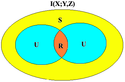
Figure 1Information exchange from two sources, Y and Z, to the target X decomposed according to PID as unique information (U), redundant information (R), and synergistic information (S).
Here we are investigating the information exchange from ENSO and IOD to ISMR interannual variability by using available observations, reanalysis datasets, and climate models. However, before exploring the two-source IE from the ENSO and IOD to ISMR variability, we first demonstrate the concept of two-source IE with results from a simple idealized linear and nonlinear dynamical models for better understanding. We also use various estimators of IE, for example linear, Kraskov, and kernel estimators, for robustness. Then, the two-source IE concept is applied to observations and reanalysis datasets. This helps in understanding the IE dynamics of ENSO and IOD to the interannual variability of ISMR in the natural system. Thereafter, we investigate if the two-source information exchange dynamics of ENSO and IOD to ISMR interannual variability are replicated in three different global climate model (GCM) simulations from the fifth phase of the Coupled Model Intercomparison Project (CMIP5). Since it is well known that GCMs due to their low spatial resolution do not resolve all the subgrid-scale phenomena, we have used dynamical downscaling of the three GCM simulations with a regional climate model (RCM) to obtain higher-resolution details (Bhaskaran et al., 2012; Chowdary et al., 2018; Dobler and Ahrens, 2011; Asharaf and Ahrens, 2015; Lucas-Picher et al., 2011). The RCM simulations are performed with a horizontal resolution of 25 km (∼0.22) and follow the framework of coordinated regional downscaling experiments (CORDEX) (Giorgi et al., 2009; Gutowski et al., 2016). By employing two-source IE from the ENSO and IOD to ISMR interannual variability on both the driving GCM simulations and the downscaled RCM simulations, we can evaluate the performance of the model chain. To our knowledge, this study is the first of its kind in evaluating GCM simulations and RCM simulations with information theory methods from the two-source IE viewpoint.
This paper is organized as follows. In Sect. 2 we briefly explain the information theory methods and estimators used in this study, followed by a brief discussion about the idealized linear and nonlinear dynamical systems. In Sect. 3, observational and reanalysis data, various GCMs in CMIP5 used in this study, and the RCM used in dynamically downscaling the GCM simulations are discussed. In Sect. 4, the results obtained from idealized systems and model evaluation are shown along with a detailed discussion. Finally, conclusions are drawn in Sect. 5.
Shannon (1948) introduced the concept of information entropy, which quantifies the average uncertainty of a given random variable. Recently, various methods from information theory have been widely used in the fields of Earth system sciences (Bennett et al., 2019; Gerken et al., 2019; Jiang and Kumar, 2019; Ruddel et al., 2019), climate sciences (Nowack et al., 2020; Runge et al., 2019; Joshua et al., 2019; Campuzano et al., 2018; Bhaskar et al., 2017), and other interdisciplinary sciences (Wibral et al., 2017; Leonardo et al., 2019; Shoaib, 2018). This section comprises the basic concepts of information theory along with a brief introduction of various estimators. Also, a description of the idealized systems used in this study is covered.
2.1 Concepts from information theory
The Shannon entropy (Shannon, 1948) of a random variable X quantifies the amount of uncertainty contained in it and is defined by
where p(x) is the probability of a discrete state of the random variable X. The summation goes through all states of the random variable X. The units of entropy are expressed in nats if a natural logarithm is applied (in bits when the logarithm base is 2).
Mutual information (MI) quantifies the reduction in the uncertainty of one random variable given knowledge of another variable (Cover and Thomas, 1991) and is defined by
where p(x, y) is the joint distribution of variables X and Y, and p(x) and p(y) are the marginal distributions of X and Y, respectively.
Mutual information between two sources Y and Z and a target X is given as
where p(x, y, z) is the joint distribution of variables X, Y, and Z, and p(x) and p(y, z) are the marginal probabilities. Furthermore, the information I(X; Y, Z) that the two sources share with the target should decompose according to partial information decomposition by Williams and Beer (2010) into four parts (Fig. 1) as
where U(X; is the unique information shared by Y to X, U(X; is the unique information shared by Z to X, R(X; Y, Z) is redundant information shared by both sources Y and Z together with X, and S(X; Y, Z) is synergistic information about X while knowing the states of Y and Z together.
In the case of two sources influencing the target, the mutual information shared by a single source to the target is given by
From the current information theory framework, the quantities I(X; Y, Z), I(X; Y), and I(X; Z) can be straightforwardly computed. Unfortunately, with the present standard methods available from information theory, one cannot obtain the contributions of unique, synergy, and redundant information exchange metrics solely (Barrett, 2015). Here, we would like to bring to the attention of the readers that many interesting studies have come up with various definitions of these metrics (Williams and Beer, 2010; Griffith and Koch, 2014; Bertschinger et al., 2014; Finn and Lizer, 2018), and there has still been no consensus among the scientific community for obtaining these metrics. A complete and consistent framework on quantifying the individual contributions of various terms in PID would make information theory a complete framework for understanding the information dynamics of multisource systems.
According to Barrett (2015), one can obtain a quantity known as net synergy from Eqs. (1) and (2) as
When ΔI(X; Y, Z)>0, synergistic information from two sources is greater than redundant information and vice versa. The ΔI provides a lower bound for synergistic and/or redundant information. From here on, if ΔI(X; Y, Z)>0 we refer to it as net synergistic information, and if ΔI(X; Y, Z)<0 we refer to it as net redundant information.
2.2 Estimation techniques
Though the information theory methods are very useful in assessing the behavior of dynamical systems, their estimation is challenging. Hence, in this study, we implemented various estimators for robustness in our results.
2.2.1 Estimation under linear approximation (linear estimator)
Here we will briefly introduce the basic concepts for estimation of two-source IE under linear approximation. For a detailed explanation of the concept, we refer the reader to Barrett (2015).
The entropy for a continuous random variable X under linear approximation is given as
where m is the dimension of random variable X, and Σ(X) is the m×m matrix covariances, i.e., cov(Xi, Xj).
Following Barrett (2015), the partial covariance of X with respect to Y is given as
From then, the conditional entropy can be derived as
The mutual information I(X; Y) is the difference between H(X) and H(X|Y),
For a general three-dimensional jointly Gaussian system (X, Y, Z)T and by setting zero mean and unit variance, the covariance matrix is given by
Thus, from the above matrix, the mutual information is given as
The net synergy can be obtained by I(X; Y, Z)−I(X; Y)−I(X; Z), given as
2.2.2 Estimation through box step kernel (kernel estimator)
The estimation of nonlinear entropy and mutual information estimators contains probability density functions (PDFs). The univariate and bivariate PDFs for continuous data can be estimated through various available discretization methods (e.g., binning, kernel). Here we use a simple box step kernel Θ with and for the estimation of relevant joint probability distributions (e.g., , y), , and ). For example, the joint probability distribution , y) is calculated as
where the norm corresponds to the maximum distance in the joint space and r is the kernel width. Similarly one can estimate the PDF for high-dimensional systems for the estimation of MI. For more details on the estimator, refer to Kantz and Schreiber (1997) and Goodwell and Kumar (2017) as well as the information-theoretic toolkit from Lizier (2014).
2.2.3 Estimation through k-nearest neighbor (Kraskov estimator)
The k-nearest neighbor estimator uses an adaptive binning strategy by estimating the average distances to the k-nearest neighbor data points. For example, the MI can be computed as
where N is total number of points, nx and ny are the number of points that fall in the marginal spaces of X and Y, respectively, within the distance taken as , ), and Ψ denotes the digamma function. For more details, refer to Kraskov et al. (2004). Similarly, the equation mentioned above can be extended to a higher-dimensional estimation of MI. Hereafter, estimation through the k-nearest neighbor is called the Kraskov estimator.
2.3 Idealized systems for demonstration
Before we apply information theory estimators to two-source information exchange in climate applications, we consider idealized linear systems as given in the following subsection to demonstrate the concept of two-source IE.
2.3.1 Linear autoregressive systems
Often in climate systems, the future state prediction of a variable relies on the past of its own state (persistence), from the past of another variable (Runge et al., 2014), or from the linear–nonlinear combination of both (possible case of net synergy and/or redundancy). Hence, as a first case of demonstration, we considered a two-dimensional linear system (Barrett, 2015) x and y, with x receiving information from its immediate past and from the immediate past of y, with the following governing equations:
where α is the coupling coefficient varied from 0 to 0.8 with an increment of 0.1, and 𝒩(0, 1) is Gaussian noise with zero mean and unit variance. The system was initialized with (x0=0) and is integrated around 100 000 iterations. For the analysis of two-source IE with various estimators, we use the last 5000 time units from the available time series.
In the first example, we considered IE from two sources (one source being the persistence) contributing to the target prediction; however, not all predictions of the target depend on two sources simultaneously (i.e., net synergy and redundancy do not exist). Hence, as a second case, we considered a system consisting of two subsystems that are coupled with each other but only having a single source with the governing equations
with α being the coupling coefficient. We followed similar steps for integration as in the previous linear system.
Finally, as a third example, we test a three-dimensional system in which two individual subsystems contribute to the evolution of the third system, such as the ENSO and IOD as two individual systems contributing to the interannual variability of ISMR. This system has the governing equations
where systems y and z are two individual subsystems exchanging information to the target system x.
We also extended our analysis to a nonlinear Heńon system described in the Appendix.
In this section, we will discuss various observational and reanalysis datasets used to quantify the two-source IE from ENSO and IOD to ISMR interannual variability in the natural system. Furthermore, the details of various GCM and RCM simulations used in this study are also covered.
3.1 Observational reanalysis datasets and climate simulations
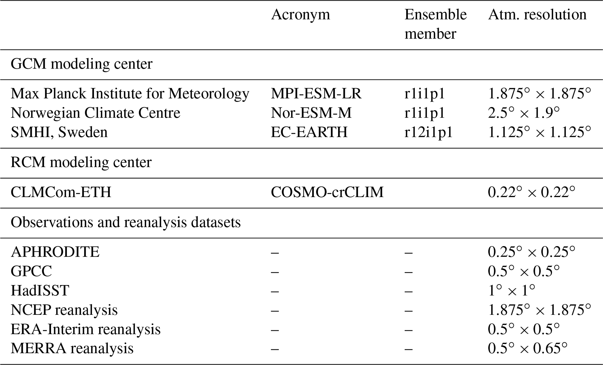
We focus on the South Asian summer monsoon seasons, starting from June and ending in September (June–July–August–September: JJAS); thus, monthly datasets for JJAS for the time period 1951–2005 from observations and model simulations are used in this study. Various observational reanalysis datasets and model simulations used to quantify two-source IE from the ENSO and IOD to ISMR interannual variability are listed in Table 1 and are also described here.
Table 1CMIP5 GCMs, RCMs, and observation descriptions used in the current study.
3.1.1 Observational reanalysis datasets and indices
The UK Met Office's Hadley Centre Sea Ice and Sea Surface Temperature dataset (HadISST 1.1) (Rayner et al., 2002) is used to retrieve SST information for the Indian and the Pacific Ocean. Monthly precipitation fields from the Global Precipitation Climatology Centre (GPCC) (Schneider et al., 2008) are used as a precipitation observational record together with a high-resolution dataset, covering only the monsoon South Asia domain, namely the Asian Precipitation–Highly-Resolved Observational Data Integration Towards Evaluation (APHRODITE) monthly accumulated precipitation (Akiyo et al., 2012). The rainfall, winds, and specific humidity are taken from the National Center for Environmental Prediction–National Center for Atmospheric Research (NCEP–NCAR) reanalysis dataset (Kalnay et al., 1996). The ENSO and IOD indices are obtained from the National Oceanic and Atmospheric Administration Earth System Research Laboratories (NOAA ESRL) and Japan Agency for Marine-Earth Science and Technology (JAMSTEC) for validation of principal components (PCs) derived from the observational SST datasets, i.e., the HadISST, and NCEP reanalysis SST. In addition to the abovementioned datasets, we also used ERA-Interim (Dee et al., 2011) and MERRA (Rienecker et al., 2011) reanalysis rainfall datasets (1980–2005) as additional resources.
3.1.2 Global and regional climate simulations
The three CMIP5 GCMs (details in Table 1), MPI-ESM-LR (Stevens et al., 2017), Nor-ESM-M (Bentsen et al., 2013), and EC-EARTH (Hazeleger et al., 2010), were dynamically downscaled with the nonhydrostatic regional climate model COSMO-crCLM version v1-1. COSMO-crCLIM is an accelerated version of the COSMO model (Fuhrer et al., 2014) in climate mode (Leutwyler et al., 2016; Rockel et al., 2008). Two-stream radiative transfer calculations are based on Ritter and Geleyn (1992), the convection is parameterized by Tiedtke (1989), the turbulent surface energy transfer and planetary boundary layer use the parameterization of Raschendorfer (2001), and precipitation is based on a four-category microphysics scheme that includes cloud, rainwater, snow, and ice (Doms et al., 2011). The soil–vegetation–atmosphere transfer uses TERRA-ML (Schrodin and Heise, 2002); however, this current version employs a modified groundwater formulation (Schlemmer et al., 2018). The RCM simulation has a horizontal resolution of 0.22∘ (i.e., 25 km) with 57 vertical levels and uses a time step of 150 s. The model simulation configuration follows the CORDEX framework, meaning that a historical period is simulated from 1950 to 2005, and the business-as-usual future emission scenario (RCP8.5) is simulated from 2006 to 2099. However, here we are only looking into the historical period. It is to be noted that for the analysis of rainfall anomaly composites, moisture anomalies, and IE plots, the GCM and RCM simulations are interpolated to a common observational grid (a grid with 0.25∘). Our interpretation of results does not change much with the original resolution of the datasets.
In the current section, we first discuss the results of two-source IE obtained from various idealized linear dynamical systems mentioned in Sect. 2. Thereafter, we present results of two-source IE in the climate system with observations, reanalysis datasets, GCM simulations, and RCM simulations.
4.1 Applications to idealized systems
First, we will start with the discussion of results obtained from idealized systems with various IE estimators.
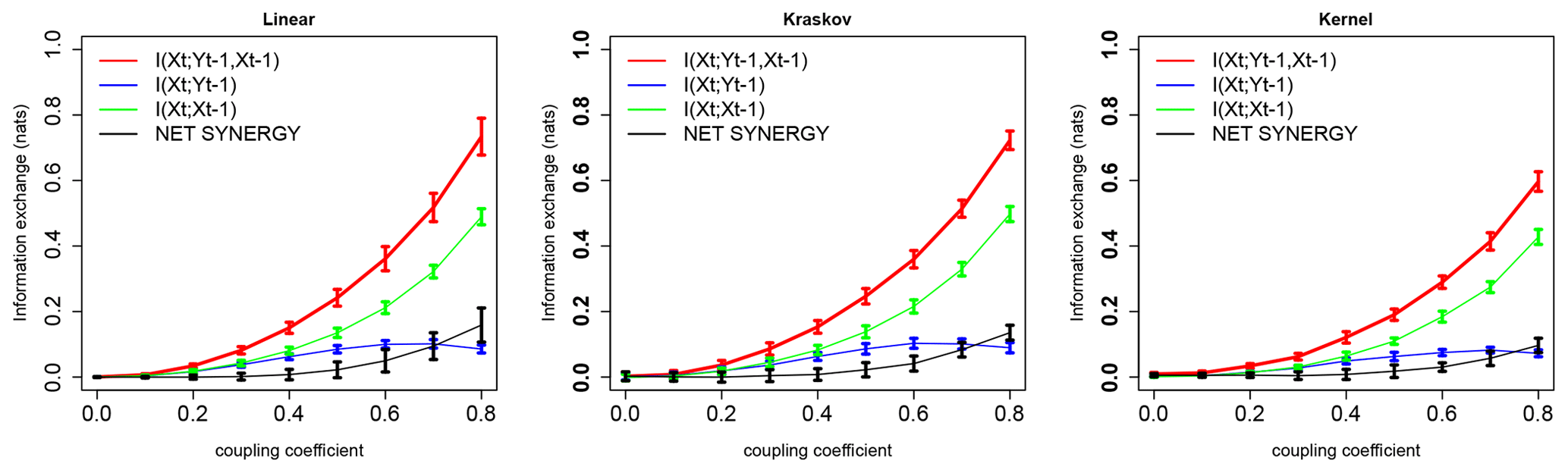
Figure 2Information exchange in nats from two sources (red line), a single source (green and blue lines), and net synergy (black line) to the target with linear, Kraskov, and kernel estimators. The error bars represent 2 standard deviations of the 100 permuted samples.
4.1.1 Linear autoregressive system
Figure 2 shows the information exchange (in nats) from yt−1 (immediate past of y) to xt (present of x) and also from x immediate past to the present of x (i.e., xt−1 to xt) for the system with Eq. (4). The two-source mutual information linear estimator shows that as the coupling coefficient increases, the IE from I(xt; yt−1, xt−1) increases, indicating that the immediate pasts of xt−1 and yt−1 exchange information to the future state of x as expected from the system dynamics. Also, as expected I(xt; yt−1, ; yt−1) or I(xt; xt−1), indicating that two-source IE dominates the dynamics of this system. The IE from the immediate past of x, i.e., xt−1, is a stronger source of information to the target xt due to self-feedback and large persistence, and yt−1 is a weaker source to the target xt (this behavior is often observed in the climate system in which persistence and self-feedback play an important role; Runge et al., 2014). The error bars represent 2 standard deviations of the 100 permuted surrogates showing the measure of uncertainty for the IE estimations. Furthermore there is a significant positive net synergy (ΔI), indicating that the two sources at higher couplings exchange synergistic information to the target even though the two sources yt−1 and xt−1 are uncorrelated with each other; in other words, a certain degree of uncertainty about the system xt is reduced by knowing the state of xt−1 and yt−1 together. Here in this system, the synergy between the two sources (yt−1 and xt−1) to the prediction of the target (xt) might be arising from their linear combination. This shows that linear systems can exhibit synergies, which is also shown analytically in the work by Barrett (2015). The nonlinear estimators, i.e., the Kraskov estimator (40 k-nearest neighbors) and kernel estimator (a kernel width of 1.5), also show similar system behavior. The free parameters, i.e., kernel width (a kernel width of 1–2) and the number of k-nearest neighbors (20–60 neighbors), are tested and tuned for consistent and robust results.
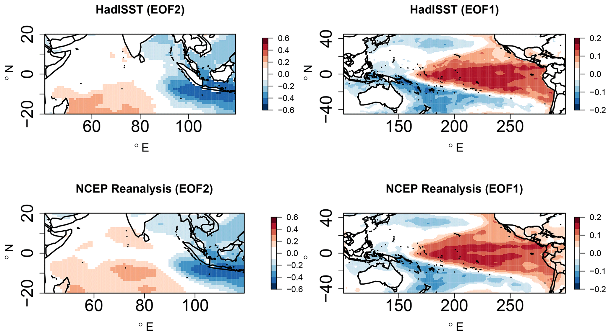
Figure 3EOF2 patterns of SST anomalies (JJAS) in the Indian Ocean and EOF1 patterns in the Pacific Ocean for observed HadISST and NCEP reanalysis.
Next, we tested another system consisting of two subsystems coupled with each other but only having a single source as in Eq. (5). From Fig. S1 (in the Supplement), the MI linear metrics show that I(xt; ; yt−1, xt−1), indicating that the immediate pasts of xt−1 does not contribute to IE for the target xt. The net synergy from to the target xt is as expected zero. The IE from yt−1 to xt increases as the coupling coefficient increases, which is also expected. This is also seen in the Kraskov estimator (40 k-nearest neighbors) and kernel estimator (a kernel width of 1.5). The free tuning parameters are tested and tuned for consistent results. Finally, among the linear systems, we tested a three-dimensional system (similar to the situation of ENSO and IOD influencing ISMR variability) with Eq. (6). Figure S2 shows the information exchange from I(xt; ; zt−1), indicating that the two sources contribute to the target system equally, and moreover the IE increases with an increase in the coupling coefficient. This behavior is expected as observed from the governing equations. Even though the two sources are uncorrelated with each other, they exhibit positive net synergy. The similar behavior in the system is seen with the nonlinear kernel estimator (a kernel width of 1.5) and Kraskov estimator (40 k-nearest neighbors). The free parameters are tested and tuned for consistent results. The results for the nonlinear system are discussed in Appendix.
The results from idealized linear and nonlinear examples show that some systems do exhibit positive net synergy from two sources to the target for both linear and nonlinear systems, even when the two sources are uncorrelated. Furthermore, all three estimators mentioned above, i.e., linear, kernel, and Kraskov estimators, are able to consistently detect two-source information exchange.
4.2 Application of dual-source IE to climate phenomenon
In this section, we examine the two-source IE from ENSO and IOD to the interannual variability of ISMR. Foremost, we present results obtained from the observational reanalysis datasets and then extend our analysis of two-source IE to three GCM simulations as mentioned in Table 1. Thereafter, we present results from our dynamically downscaled simulations with COSMO-crCLM with the three GCMs as driving models.
4.2.1 Observation and reanalysis data
In the observations and reanalysis datasets, empirical orthogonal function (EOF) analysis of the detrended SST anomalies is performed over the tropical Indian Ocean (25∘ S–20∘ N, 50–120∘ E) and the tropical Pacific Ocean (25∘ S–25∘ N, 120∘ E–80∘ W) to obtain the major oscillations and their respective PCs. The ENSO and IOD indices are taken as the time series associated with their respective PCs obtained from the EOF spatial patterns replicating them. Figure 3 shows the second EOF patterns of the SST anomalies over the Indian Ocean and the first EOF patterns over the Pacific Ocean for HadISST and from the NCEP reanalysis. From the two SST datasets, it is observed that both ENSO- and IOD-like structures are captured with the second EOF and the first EOF patterns, i.e., a zonal dipole-like structure in the Indian Ocean and the Pacific Ocean, respectively. We use EOF analysis as opposed to standard indices such as the dipole mode index, known as DMI (Saji et al., 1999), and Niño 3.4 to allow each model to exhibit its own patterns as opposed to an imposed structure (Saji et al., 2006; Cai et al., 2009a, b; Liu et al., 2011).

Figure 4Total precipitation anomaly (millimeters per month) composites (JJAS) over the Indian subcontinent for El Niño, La Niña, and positive IOD and negative IOD events observed in GPCC, APHRODITE, and NCEP reanalysis datasets for the period of 1951–2005.
To ensure that the EOF patterns in the observed SST datasets replicate the ENSO and IOD modes, the obtained PCs are compared against the corresponding Niño 3.4 and IOD index obtained from the NOAA ESRL Physical Sciences Division and JAMSTEC observations (shown in Fig. S3). These indices are widely used in several studies concerning IOD and Niño 3.4 teleconnections. The percentage of the total variance contributed by the first 20 EOFs from the Indian and Pacific Ocean SST anomalies for JJAS are also shown in Fig. S3. The linear fit between the Indian Ocean PCs of EOF2 obtained from the HadISST against the observed IOD index has a correlation of about 0.78, and the correlation of NCEP reanalysis SST with the observed IOD index is 0.77. These results are significant at a 99 % confidence level. This indicates that EOF2 replicates the IOD-like variability for the two mentioned datasets. The percentage of the total variability contributed by EOF1 for the Indian Ocean is about 30 %, which is associated with the basin-scale anomalies of uniform polarity in the Indian Ocean associated with ENSO events. The dipole mode (EOF2) explains about 15 % of the total variance, which is associated with the IOD. Our results for the Indian Ocean EOF patterns and their respective contribution to the total variance are consistent with the study by Saji et al. (1999). Similarly, the PCs associated with the first EOF over the Pacific Ocean are highly correlated against the observed Niño 3.4 index, with a correlation value greater than 0.8 for both datasets, indicating that EOF1 captures the ENSO-like variability. The percentage of total variance contributed by the first EOF, ≈20 %, is also consistent with the ENSO literature.
The ENSO and IOD are known to influence the ISMR distribution across the Indian subcontinent. Hence, to investigate the rainfall anomaly distribution during various phases of ENSO and IOD (i.e., El Niño, La Niña, IOD+ve, and IOD−ve), we plotted the anomaly composite figures (Fig. 4) for ISMR during these events. The anomalies are constructed by subtracting the Indian subcontinent climatology mean JJAS rainfall with the rainfall months associated with various phases of IOD and ENSO. The anomaly composites with El Niño (La Niña) events show that most parts of the Indian subcontinent receive less (more) rainfall during El Niño (La Niña) phases. This behavior can be attributed to the suppression of convection over the Indian subcontinent during the El Niño phase through the zonal and meridional circulation and vice versa during a La Niña phase. The rainfall anomaly composites associated with the positive and negative phases of the IOD represent distinct regional asymmetric rainfall anomalies, i.e., a meridional tripolar pattern, with above-normal rainfall in central parts of India and below-normal rainfall to the north and south of it. Conversely, the negative IOD is associated with a zonal dipole having above-normal (below-normal) rainfall on the western (eastern) half of the Indian subcontinent. These results with rainfall composites during IOD phases are consistent with Behera and Ratnam (2018), wherein it was concluded that these rainfall anomaly patterns are due to differences in atmospheric responses and the associated differences in moisture transport to the region during contrasting phases of the IOD. Hence, Fig. 4 indicates that both ENSO and IOD contribute to the interannual variability of ISMR.
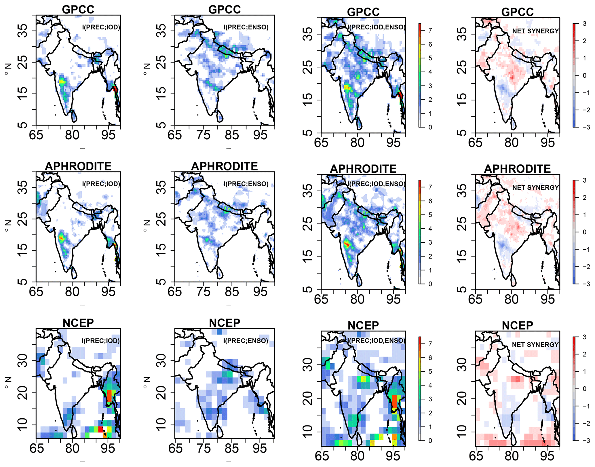
Figure 5Information exchange from I(PREC; IOD), I(PREC; ENSO), two-source information exchange I(PREC; ENSO, IOD), and net synergy × 10−2 nats for the observational datasets GPCC, APHRODITE, and NCEP reanalysis. Only significant values at 95 % confidence intervals are plotted.
Figure 5 represents the IE from the IOD to precipitation, i.e., I(PREC; IOD), ENSO to precipitation, i.e., I(PREC; ENSO), and two-source IE, i.e., I(PREC; IOD, ENSO), together with the net synergy for the observations GPCC, APHRODITE, and the NCEP reanalysis datasets under linear approximation. We chose various precipitation datasets to accommodate uncertainties due to the sparse data networks, especially in regions with complex topography. The observed IE from IOD to total precipitation, i.e., I(PREC; IOD), shows that the IOD transmits information to the southwest sector of the Indian subcontinent, especially the leeward side of the Western Ghats region, in the GPCC and APHRODITE datasets. This feature is slightly shifted to the east in the NCEP reanalysis datasets. All the IE plotted values are significant at the 95 % confidence level obtained from 100 surrogate samples. Some regions in the northeast sector also are influenced by IE from IOD, which is replicated in all three observational datasets. It is interesting to note that the location at which IE from IOD to the precipitation over the Indian subcontinent matches the significant rainfall anomalies shown in Fig. 4. The I(PREC; ENSO) shows that the northern parts of the Himalayas in central India receive information from the Pacific Ocean in all three datasets; this also matches the anomaly locations shown in Fig. 4. The two-source information exchange covers most parts of the Indian subcontinent, indicating that both ENSO and IOD contribute to ISMR during JJAS. Also, interestingly from the net synergy plot, a positive net synergy over certain parts of central India, also known as the monsoon core region, is observed, indicating that both ENSO and IOD synergistically contribute to the interannual variability of ISMR. Furthermore, the ENSO and IOD share net redundant information (negative net synergy) in the southern sector of the Indian subcontinent. The Kraskov estimator (Fig. S4) and the kernel estimator (Fig. S5) also show similar IE patterns over the Indian subcontinent, with 40 k-nearest neighbors for Kraskov and a 0.5 kernel width for kernel estimators (free parameters are tested and tuned for consistent results). In addition, we also checked the two-source IE patterns in the two reanalysis datasets, MERRA and ERA-Interim (1980–2005), shown in Figs. S6 and S7. It is found that in both the datasets, similar IE patterns are replicated, i.e., positive net synergy in central India and net redundant information in the southern part of the Indian subcontinent. We also did a similar analysis for the months of DJFM, and our results show that the net synergy from IOD and ENSO to rainfall is absent (Figs. S8–S13). This is expected as the IOD mode during these months is dissipated and absent.
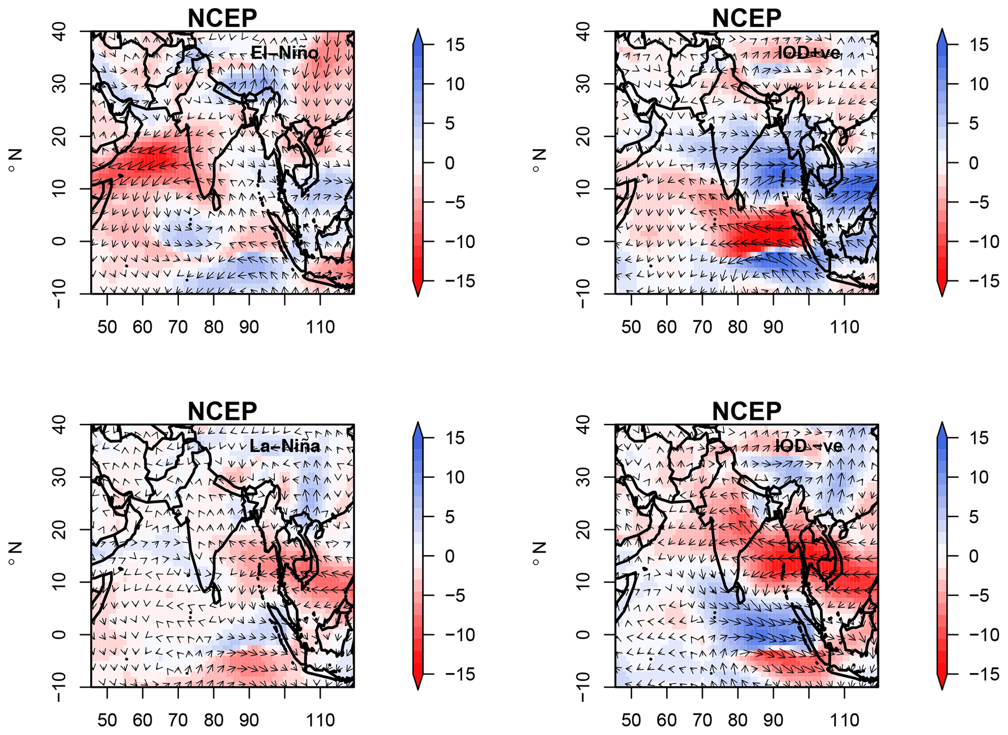
Figure 6Moisture flux anomalies (g kg−1 m s−1) over the Indian subcontinent (JJAS) for El Niño, La Niña, IOD+ve, and IOD−ve events observed in NCEP reanalysis datasets for the period of 1951–2005.
The net synergy between the ENSO and IOD to ISMR interannual variability in JJAS indicates that central Indian monsoon rainfall predictability lies in knowing the states of ENSO and IOD together rather than by knowing the states of ENSO and IOD individually (similar to the idealized test case example 3). This is also similar to the XOR logic gate, whereby the uncertainty of the output is known only with simultaneous knowledge of the two input states. To understand the information synergy physically, we show the moisture transport figures from the NCEP reanalysis datasets for various phases of ENSO and IOD during JJAS. From Fig. 6 it is observed that the anomalous negative moisture flux during El Niño is compensated for by the positive moisture flux anomaly by IOD+ve, especially in central India, and vice versa during La Niña and IOD−ve events. It is known that El Niño events are often associated with IOD+ve events (Behera and Ratnam, 2018) and vice versa (the ENSO and IOD are positively correlated in our datasets). From the precipitation composites (Fig. 3), in central India, anomalous negative (positive) rainfall during El Niño (La Niña) is observed, and during IOD+ve (IOD−ve) positive (partly negative) anomalous rainfall is observed. This could explain why both the IOD and ENSO states should be known together to explain the variability of central Indian subcontinent rainfall, as the IOD and ENSO have compensating effects. This compensating behavior is not seen in the southern or northern part of the Indian subcontinent; hence, this could explain the net redundant information between ENSO and IOD to the precipitation in the southern region. Readers are referred to Fig. 3 by Barrett (2015) to further explore the relation of synergy dependence to the compensating influence from both sources, i.e., the correlation between two sources and their targets.

Figure 7EOF2 patterns of SST anomalies (JJAS) in the Indian Ocean and EOF1 patterns (JJAS) in the Pacific Ocean for three GCM simulations, i.e., MPI-ESM-LR, Nor-ESM-M, and EC-EARTH, for the period of 1951–2005.
4.2.2 Global and regional climate model simulations
Next, we perform the same analysis, starting with the EOF patterns from the SST fields obtained from the three GCM simulations listed in Table 1, to investigate how the ENSO- and IOD-associated variability in the Indian and Pacific oceans is represented. Figure 7 shows the second EOF pattern of the SST anomalies over the Indian Ocean and the first EOF pattern in the Pacific Ocean for the GCM simulations of MPI-ESM-LR, Nor-ESM-M, and EC-EARTH. It is found that all the GCM simulations replicate the zonal dipole-like patterns over the Indian Ocean and Pacific Ocean, similarly to the observations. The percentage of the total variability contributed by EOF1 for the Indian Ocean is about 30 % in all the GCM simulations (Fig. S14), which is comparable to the observations. EOF2, which is associated with the IOD, explains about 15 % of the total variance in all the GCMs, also similar to observations. The percentage of total variance contributed by the first EOF is between 20 % and 25 % in all the GCM simulations in the Pacific Ocean, which is similar to variance in the observations. Thus, these results indicate that the variability associated with the SST anomalies over the Indian and Pacific Ocean is represented in the three GCM simulations. The SST anomaly composites during various phases of IOD and ENSO events (Figs. S15 and S16) show that most of the GCM simulations can replicate the SST anomaly composite patterns found during IOD+ve events in HadISST (Fig. S15). In contrast, during IOD−ve events, MPI-ESM-LR portrays unrealistic warm anomalies throughout the Indian Ocean. Over the Pacific Ocean, MPI-ESM-LR and EC-EARTH have an unrealistic westward extension of the warm (cold) pool during El Niño (La Niña) events. The patterns from Nor-ESM-M are closer to the observations, as shown in Fig. S16. The unrealistic westward extension of the SSTs in EC-EARTH and MPI-ESM-LR simulations might influence the Walker circulation through unrealistic large-scale teleconnection patterns.
Figure 8 represents the ISMR anomaly composites during El Niño, La Niña, IOD+ve, and IOD−ve events for the three GCM simulations MPI-ESM-LR, Nor-ESM-M, and EC-EARTH when selecting the associated years given by the respective PCs. The rainfall anomaly composites associated with the positive phase of ENSO show dry conditions over the northern–northwest parts of the Indian subcontinent in MPI-ESM-LR and dry conditions throughout the Indian subcontinent in Nor-ESM-M. The EC-EARTH simulation does not show a clear rainfall anomaly signal. Similar opposite polarity of rainfall anomalies is observed in La Niña conditions in the MPI-ESM-LR and Nor-ESM-M simulations, while slight wet conditions are seen in northeast India in EC-EARTH. For IOD+ve events, MPI-ESM-LR shows dry conditions in the southwest, while the Nor-ESM-M simulation shows dry conditions in the northwest and the Himalayan region; EC-EARTH does not show any variability. Nor-ESM-M during the IOD−ve phase shows an overall positive anomaly, while no clear signal is observed in MPI-ESM-LR and EC-EARTH. Overall, the ENSO phase signal is better replicated in the Nor-ESM-M simulation and partly in MPI-ESM-LR as in the observations, while most of the GCM simulations failed to replicate the regional rainfall asymmetric response in IOD events as in observations (except Nor-ESM-M, which can partly replicate the dipole patterns). This might be due to the coarse resolution of GCMs, which may not be able to replicate the fine-scale precipitation response to the IOD.
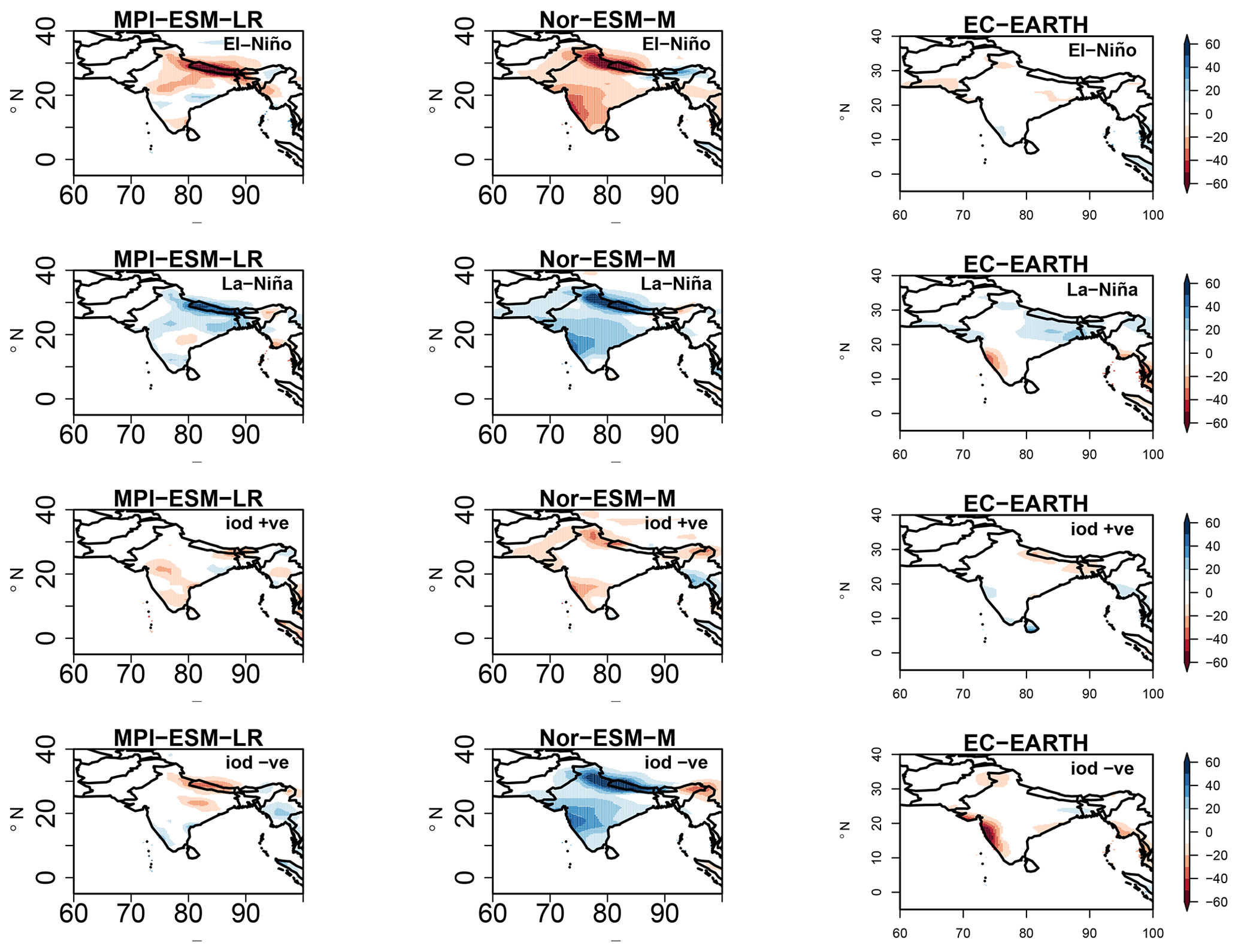
Figure 8Total precipitation anomaly composites over the Indian subcontinent (JJAS) for El Niño, La Niña, and positive IOD and negative IOD events in MPI-ESM-LR, Nor-ESM, and EC-EARTH simulations (1951–2005).
Figure 9 represents the IE spatial patterns from the IOD and ENSO, i.e., I(PREC; IOD), I(PREC; ENSO), the two-source IE, and I(PREC; IOD, ENSO), together with the net synergy over the Indian subcontinent in the three GCM simulations, i.e., MPI-ESM-LR, Nor-ESM-M, and EC-EARTH, with the linear estimator. The information exchange from IOD to total precipitation in MPI-ESM-LR shows that the information from the IOD is exchanged to the southeastern part of the Indian subcontinent. This is contrary to what is seen in the results from the observations, wherein most of the IE takes place to the leeward side of the Western Ghats and the northeastern sector of India. The Nor-ESM-M simulation shows that IE from IOD is transmitted to the western side of the Indian subcontinent, where the observed significant anomalies are noted in Fig. 9. EC-EARTH does not show any information exchange from IOD to the land points over the Indian subcontinent. I(PREC; ENSO) shows that the northern parts of the Himalayas and northwest–central India receive information from the Pacific Ocean in MPI-ESM-LR. For Nor-ESM-M, the Western Ghats and its leeward side are influenced by ENSO. EC-EARTH does not show as much IE as Nor-ESM-M or MPI-ESM-LR over the Indian continent, with an exception for some scattered locations over the Himalayas.
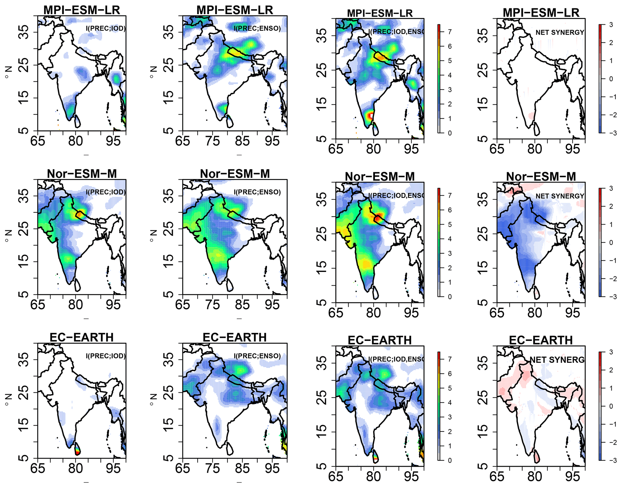
Figure 9Information exchange from I(PREC; IOD), I(PREC; ENSO), two-source information exchange I(PREC; ENSO, IOD), and net synergy × 10−2 nats for the GCM simulations MPI-ESM-LR, Nor-ESM-M, and EC-EARTH for JJAS (1951-2005). Only significant values at 95 % confidence intervals are plotted.
The two-source information exchange I(PREC; ENSO, IOD) covers the northwest part of the Indian subcontinent for MPI-ESM-LR and the extreme southeast. For Nor-ESM-M the information exchange covers mostly the western part of India. EC-EARTH shows IE over isolated places in northeast India. These results indicate that the three GCMs exhibit an IE pattern that is different from the observed patterns. Moreover, the results for net synergy show that MPI-ESM-LR does not show any net synergistic IE over the Indian subcontinent, while in Nor-ESM-M the IOD and ENSO share common information over the west of India. EC-EARTH shows less net synergy over the Indian subcontinent. Overall, the results from the IE exchange differ from the observations seen for all three GCM simulations. These results are consistent with kernel and Kraskov estimators (Fig. S17).
Next, we investigate how two-source information exchange is represented when we dynamically downscale the three GCM simulations (MPI-ESM-LR, Nor-ESM-M, and EC-EARTH) with the regional model COSMO-crCLIM (0.22∘). We apply the same two-source information exchange method to the RCM fields as for the GCM simulations. However, since the RCM simulations only cover a limited area, namely the South Asian CORDEX domain, we had to combine the RCM results with the GCM simulations, in particular for the EOF analysis over the Indian and Pacific oceans. Figure 10 represents the ISMR anomaly composites during positive IOD+ve, IOD−ve, El Niño, and La Niña events for the COSMO-crCLM RCM simulation driven with three GCM simulations, MPI-ESM-LR, Nor-ESM-M, and EC-EARTH. Here we select the same years as given by the principal components from the driving GCM simulations. The rainfall anomaly composites associated with El Niño events show dry conditions over the northern parts of the Himalayas for the downscaled MPI-ESM-LR and wet conditions in Western Ghats and isolated parts of central India. During the La Niña phase, dry conditions are observed in the central Indian subcontinent and Western Ghats, and wet conditions are observed elsewhere. In the downscaled Nor-ESM-M, a dry (wet) signal is observed throughout the Indian subcontinent during El Niño (La Niña) phases. In the downscaled EC-EARTH, dry regions are noted throughout most parts of the Indian subcontinent during El Niño, while dry conditions are seen in central India and wet conditions elsewhere in the La Niña phase. The rainfall anomaly composites associated with the positive IOD in the observations, i.e., a meridional tripolar pattern with above-normal rainfall in central parts of India and below-normal rainfall to the north and south of it, are only observed in the downscaled Nor-ESM-M. Similarly, the negative IOD in downscaled Nor-ESM-M is associated with a zonal dipole having above-normal (below-normal) rainfall on the western (eastern) half of India, similar to the observations as seen in Fig. 5. Overall, these results suggest that the downscaled results from Nor-ESM-M better reproduce the spatial patterns of precipitation anomalies associated with ENSO and IOD compared to the observations than the downscaled results from EC-EARTH and MPI-ESM-LR.

Figure 10Total precipitation anomaly composites over the Indian subcontinent for El Niño, La Niña, and positive IOD and negative IOD events for the downscaled COSMO-crCLM simulations driven by MPI-ESM-LR, Nor-ESM-M, and EC-EARTH GCM simulations for JJAS (1951–2005).
Figure 11 represents the IE patterns over the Indian subcontinent for the downscaled RCM simulations with the linear estimator (these patterns are also consistent with Kraskov and kernel estimators; Figs. S18 and S19, respectively). The net synergy in central India and shared information in southern India are better represented in the downscaled Nor-ESM-M simulation compared to the downscaled MPI-ESM-LR and downscaled EC-EARTH. This is in agreement with the results from the GCM simulation, in which it was found that the Nor-ESM-M simulation had a better replication of ENSO- and IOD-induced anomalous precipitation structures than the two other GCMs (see Fig. 10). These results are interesting; even though all the COSMO-crCLM simulations have the same physics and dynamics, only downscaled Nor-ESM-M replicated realistic patterns of IE. The improvement in results in downscaled Nor-ESM-M can be attributed to more realistic large-scale information coming from the GCM simulation, such as the moisture flux transport during various phases of ENSO and IOD events (see Figs. S20–S24 and 6). For the MPI-ESM-LR and EC-EARTH GCM simulations, the moisture flux anomalies are very different from the reanalysis fluxes and thus seem misrepresented. A better replication of the moisture flux anomaly in the Nor-ESM-M GCM simulation during ENSO and IOD might be from a better simulation of the large-scale circulation patterns, like the Walker and Hadley circulations, due to the better representation of the SST than the two other GCM simulations (Figs. S8 and S9). The RCM simulation results exhibit similar moisture flux anomalies compared to the driving GCM simulations, in which the downscaled Nor-ESM-M outperforms the downscaled MPI-ESM-LR and downscaled EC-EARTH. These results indicate that a realistic large-scale signal from the GCM simulations (e.g., the moisture transport and SST anomalies) is essential for an RCM to properly improve the GCM results in terms of ISMR variability. When the large-scale signal from the GCM is incorrect and wrong moisture fluxes are imposed on the lateral boundaries of the RCM, the downscaled results are hampered.
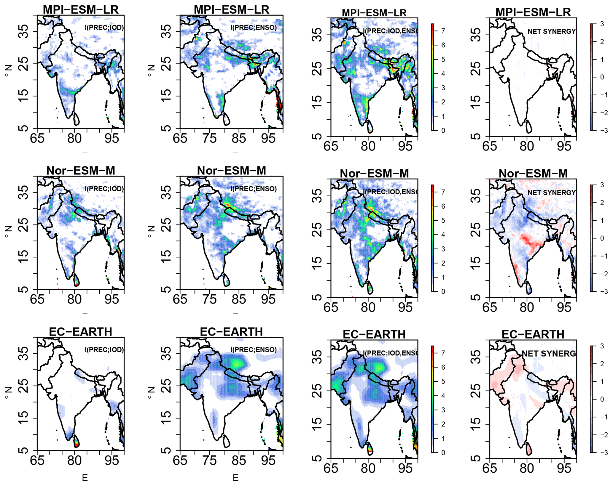
Figure 11Information exchange from I(PREC; IOD), I(PREC; ENSO), two-source information exchange I(PREC; ENSO, IOD), and net synergy × 10−2 nats for the downscaled COSMO-crCLM simulations for JJAS (1951–2005). Only significant values at 95 % confidence intervals are plotted.
In this article, we explored two-source information exchange (IE) from ENSO and IOD (quantified by SST variabilities in the Pacific and Indian oceans) to Indian summer monsoon rainfall (ISMR) interannual variability. But we first used simple idealized linear and nonlinear dynamical systems to demonstrate the concepts of two-source IE. Results showed that both the linear and nonlinear idealized systems can exhibit positive net synergy (i.e., the combined influence of two sources is greater than their individual contributions). Interestingly, two uncorrelated sources can show positive net synergistic IE to a target.
The two-source ENSO and IOD to ISMR IE was explored in observations, reanalysis datasets, and in three GCM simulations, which were also further dynamically downscaled with the RCM. The results from the observations and reanalysis data suggest that both IOD and ENSO influence the interannual variability of ISMR throughout most parts of the Indian subcontinent. Interestingly, we found that IOD and ENSO exhibit positive net synergy over central India, which is the monsoon core region, and net redundant information over the southern part of India.
The IE patterns in the three GCM simulations differ from those in the observations. However, the GCM Nor-ESM-M better captured the precipitation anomalies from ENSO and partly from IOD than the other two GCMs. Previous studies also showed that Nor-ESM-M outperforms other CMIP5 GCM simulations in terms of rainfall climatology, as well as most aspects of the climatological annual cycle and interannual variability in the Indian subcontinent (Sperber et al., 2012; McSweeney et al., 2015).
Downscaling the Nor-ESM-M simulation with the RCM COSMO-crCLM better replicated the observed IE patterns than downscaling the MPI-ESM-LR and EC-EARTH simulations. Importantly, the downscaled Nor-ESM-M IE results are in better agreement with the observations than the Nor-ESM-M results. Downscaling Nor-ESM-M adds value to the GCM simulation. This cannot be concluded here for downscaling of MPI-ESM-LR and EC-EARTH simulations. Downscaling the latter simulations did not add value because of missing realism in their large-scale SST patterns and horizontal moisture flux variability, which are important RCM boundary conditions that were better represented in the Nor-ESM-M simulation. Downscaling did not compensate for errors in the large-scale driving simulations. These results highlight the importance of the choice of GCM simulations when performing dynamical downscaling for high-resolution regional climate projections.
Finally, we propose using the two-source IE metric as a complementary tool to gain additional insight into the climate system and to perform process-oriented climate model evaluation.
As the climate system is nonlinear, we further extend our analysis from idealized linear systems to an idealized nonlinear system. For this purpose, we considered coupled Heńon maps, which capture the stretching and folding dynamics of chaotic systems such as the Lorenz system that mimics atmospheric behavior. We considered two Heńon maps (Kraskovska, 2019): x and y coupled with each other with the governing equations
where the coupling coefficients C∈[0, 0.6]. From Eq. (A1) it is evident that system x is driving system y through coupling coefficient C.
Figure A1 shows information exchange in the nonlinear Heńon system (equations given as in Eq. A1). Figure A1 shows that the IE I(yt; xt−1) increases as the coupling coefficient C increases. It can be also observed that the opposite behavior, i.e., information exchange from I(yt; yt−1), decreases with increasing C due to the term in Eq. (4). Also, the IE from I(yt; ; xt−1) indicates that the target is tightly coupled with its own past (also seen in governing equations). In this case, the two-source IE is greater than I(yt; yt−1) or I(yt; xt−1) as expected; this is because both sources are contributing to the target future state. Here the correlation between the two sources xt−1 and yt−1 is almost equal to zero. The net synergy increases with an increase in the coupling coefficient, indicating net synergistic IE by the two sources. For this system we used eight k-nearest neighbors for the Kraskov estimator and a 0.5 kernel width for the kernel estimator.
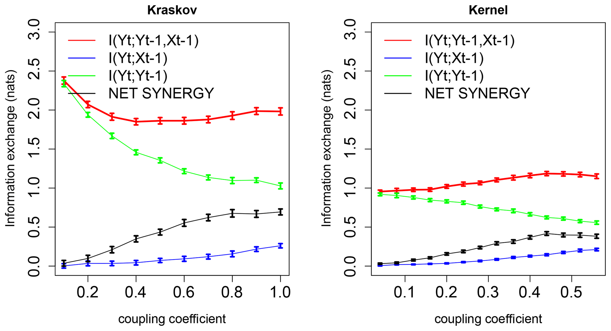
Figure A1Information exchange in nats from two sources (red line), a single source (green and blue lines), and net synergy (black line) to target for Kraskov and kernel estimators. The error bars represent 2 standard deviations of the 100 permuted samples.
The analysis is done in R, and the codes can be accessed through https://doi.org/10.5281/zenodo.4192441 (Pothapakula, 2020).
The GCM and RCM datasets are available at https://esgf-data.dkrz.de/projects/esgf-dkrz/ (last access: 2 November 2020) (ESGF, 2020). The ENSO and IOD index are taken from http://www.esrl.noaa.gov/psd (last access: 2 November 2020) (PSL, 2020) and http://www.jamstec.go.jp/ (last access: 2 November 2020) (JAMSTEC, 2020), respectively.
The supplement related to this article is available online at: https://doi.org/10.5194/esd-11-903-2020-supplement.
The concept was proposed by BA. Funding was acquired by BA. The information theory algorithms were developed by PKP and CP. The RCM simulations were performed by SS with assistance from PKP. The paper was written by PKP and reviewed by BA, SS, and CP. All authors have read and approved the final paper.
The authors declare that they have no conflict of interest.
The authors acknowledge support from the German Research Foundation (Deutsche Forschungsgemeinschaft, DFG) within the research group FOR 2416: Space–Time Dynamics of Extreme Floods (SPATE). The authors also thank Joseph T. Lizer for providing the JDIT open-source toolkit. CLMcom-ETH-COSMO-crCLIM-v1-1 simulations were run on Piz Daint at CSCS (Switzerland), and we acknowledge PRACE for granting us access and computing time. We thank two reviewers for their constructive comments and insights.
This open-access publication was funded
by the Goethe University Frankfurt.
This paper was edited by Ben Kravitz and reviewed by Benjamin L. Ruddell and Didier Vega-Oliveros.
Akiyo, Y., Kamiguchi, K., Arakawa, O., Hamada, A., Yasutomi, N., and Kitoh, A.: APHRODITE: Constructing a Long-Term Daily Gridded Precipitation Dataset for Asia Based on a Dense Network of Rain Gauges, B. Am. Meteorol. Soc., 93, 1401–1415, https://doi.org/10.1175/BAMS-D-11-00122.1, 2012. a
Ashok, K., Guan, Z., and Yamagata, T.: Impact of the Indian Ocean Dipole on the relationship between Indian monsoon rainfall and ENSO, Geophys. Res. Lett., 28, 4499–4502, https://doi.org/10.1029/2001GL013294, 2001. a, b
Asharaf, S. and Ahrens, B.: Indian Summer Monsoon Rainfall Feedback Processes in Climate Change Scenarios, J. Climate, 28, 5414–5429, https://doi.org/10.1175/JCLI-D-14-00233.1, 2015. a
Barrett, A.: Exploration of synergistic and redundant information sharing in static and dynamical Gaussian systems, Phys. Rev. E, 91, 1539–3755, https://doi.org/10.1103/PhysRevE.91.052802, 2015. a, b, c, d, e, f, g
Behera, S. K. and Ratnam, J. K.: Quasi-asymmetric response of the Indian summer monsoon rainfall to opposite phases of the IOD, Scient. Rep., 8, 123, https://doi.org/10.1038/s41598-017-18396-6, 2018. a, b, c
Bennett, A., Nijssen, B., Ou, G., Clark, M., and Nearing, G.: Quantifying process connectivity with transfer entropy in hydrologic models, Water Resour. Res., 55, 4613–4629, https://doi.org/10.1029/2018WR024555, 2019. a
Bentsen, M., Bethke, I., Debernard, J. B., Iversen, T., Kirkevåg, A., Seland, Ø., Drange, H., Roelandt, C., Seierstad, I. A., Hoose, C., and Kristjánsson, J. E.: The Norwegian Earth System Model, NorESM1-M – Part 1: Description and basic evaluation of the physical climate, Geosci. Model Dev., 6, 687–720, https://doi.org/10.5194/gmd-6-687-2013, 2013. a
Bertschinger, N., Rauh, J., Olbrich, E., Jost, J., and Ay, N.: Quantifying unique information, Entropy, 16, 2161–2183, https://doi.org/10.3390/e16042161, 2014. a
Bhaskar, A., Ramesh, D. S., Vichare, G., Koganti, T., and Gurubaran, S.: Quantitative assessment of drivers of recent global temperature variability: an information theoretic approach, Clim. Dynam., 49, 3877–3886, https://doi.org/10.1007/s00382-017-3549-5, 2017. a
Bhaskaran, B., Ramachandran, A., Jones, R., and Moufouma‐Okia, W.: Regional climate model applications on sub-regional scales over the Indian monsoon region: the role of domain size on downscaling uncertainty, J. Geophys. Res.-Atmos., 117, D10113, https://doi.org/10.1029/2012JD017956, 2012. a
Cai, W., Cowan, T., and Sullivan A.: Recent unprecedented skewness towards positive Indian Ocean dipole occurrences and its impact on Australian rainfall, Geophys. Res. Lett., 36, L11705, https://doi.org/10.1029/2009GL037604, 2009a. a
Cai, W., Sullivan, A., and Cowan, T.: Rainfall teleconnections with Indo-Pacific variability in the WCRP CMIP3 models, J. Climate, 22, 5046–5071, https://doi.org/10.1175/2009JCLI2694.1, 2009b. a
Campuzano, S. A., De Santis, A., Pavon-Carrasco, F. J., Osete, M. L., and Qamili, E.: New perspectives in the study of the Earth’s magnetic field and climate connection: The use of transfer entropy, PLOS ONE, 13, e0207270, https://doi.org/10.1371/journal.pone.0207270, 2018. a
Chowdary, J. S., Bandgar, A. B., Gnanaseelan, C., and Luo, J. J.: Role of tropical Indian Ocean air-sea interactions in modulating Indian summer monsoon in a coupled model, Atmos. Sci. Lett., 16, 170–176, https://doi.org/10.1002/asl2.561, 2015. a
Choudhary, A., Dimri, A. P., and Maharana, P.: Assessment of CORDEX-SA experiments in representing precipitation climatology of summer monsoon over India, Theor. Appl. Climatol., 134, 283–307, https://doi.org/10.1007/s00704-017-2274-7, 2018. a
Cover, T. M. and Thomas, J. A.: Elements of Information Theory, Wiley, New York, NY, USA, 1991. a
Dee, D. P., Uppala, S. M., Simmons, A. J., Berrisford, P., Poli, P., Kobayashi, S., Andrae, U., Balmaseda, M. A., Balsamo, G., Bauer, P., Bechtold, P., Beljaars, A. C. M., van de Berg, L., Bidlot, J., Bormann, N., Delsol, C., Dragani, R., Fuentes, M., Geer, A. J., Haimberger, L., Healy, S. B., Hersbach, H., Hólm, E. V., Isaksen, L., Kållberg, P., Köhler, M., Matricardi, M., McNally, A. P., Monge-Sanz, B. M., Morcrette, J.-J., Park, B.-K., Peubey, C., de Rosnay, P., Tavolato, C., Thépaut, J. N., and Vitart, F.: The ERA-Interim reanalysis: configuration and performance of the data assimilation system, Q. J. Roy. Meteorol. Soc., 137, 553–597, https://doi.org/10.1002/qj.828, 2011. a
Dobler, A. and Ahrens, B.: Four climate change scenarios for the Indian summer monsoon by the regional climate model COSMO-CLM, J. Geophys. Res.-Atmos., 116, D24104, https://doi.org/10.1029/2011JD016329, 2011. a
Doms, G., Forstner, J., Heise, E., Herzog, H. J., Mironov, D., Raschendorfer, M., Reinhardt, T., Ritter, B., Schrodin, R., Schulz, J. P., and Vogel, G.: A Description of the Nonhydrostatic Regional Model LM, Part II: Physical Parameterization, DWD, available at: http://www.cosmo-model.org/ (last access: 2 November 2020), 2011. a
ESGF – Earth System Grid Federation: GCM and RCM datasets, available at: https://esgf-data.dkrz.de/projects/esgf-dkrz/, last access: 2 November 2020. a
Finn, C. and Lizier, J. T.: Pointwise Partial Information Decomposition Using the Specificity and Ambiguity Lattices, Entropy, 20, 297, https://doi.org/10.3390/e20040297, 2018. a
Fuhrer, O., Osuna, C., Lapillonne, X., Gysi, T., Cumming, B., Bianco, M., Arteaga, A., and Schulthess, T. C.: Towards a performance portable, architecture agnostic implementation strategy for weather and climate models, Supercomputing frontiers and innovations, available at: http://superfri.org/superfri/article/view/17 (last access: 2 November 2020), 2014. a
Gadgil, S.: Indian monsoon and its variability, Annu. Rev. Earth Planet. Sci., 31, 429–467, https://doi.org/10.1146/annurev.earth.31.100901.141251, 2003. a, b
Gerken, T., Ruddell, B. L., Yu, R., Stoy, P. C., and Drewry, D. T.: Robust observations of land-to-atmosphere feedbacks using the information flows of FLUXNET, NPJ Clim. Atmos. Sci., 2, 37, https://doi.org/10.1038/s41612-019-0094-4, 2019. a
Giorgi, F., Jones, C. and Asrar, G. R.: Addressing climate information needs at the regional level: the CORDEX framework, World Meteorol. Organ. Bull., 58, 175–183, 2009. a
Goodwell, A. and Kumar, P.: Temporal Information Partitioning Networks (TIPNets): A process network approach to infer ecohydrologic shifts, Water Resour. Res., 53, 5899–5919, https://doi.org/10.1002/2016WR020218, 2017. a
Goswami, B. N.: Inter-annual variations of Indian summer monsoon in a GCM: External conditions versus internal feedbacks, J. Climate, 11, 501–522, https://doi.org/10.1175/1520-0442(1998)011<0501:IVOISM>2.0.CO;2, 1998. a, b
Goswami, B. N., Madhusoodanan, M. S., Neema, C. P., and Sengupta, D.: A physical mechanism for North Atlantic SST influence on the Indian summer monsoon, Geophys. Res. Lett., 33, L02706, https://doi.org/10.1029/2005GL024803, 2006. a
Griffith, V. and Koch, C.: Quantifying Synergistic Mutual Information, in: Guided Self-Organization: Inception. Emergence, Complexity and Computation, vol. 9, edited by: Prokopenko, M., Springer, Berlin, Heidelberg, https://doi.org/10.1007/978-3-642-53734-9_6, 2014. a
Gutowski Jr., W. J., Giorgi, F., Timbal, B., Frigon, A., Jacob, D., Kang, H.-S., Raghavan, K., Lee, B., Lennard, C., Nikulin, G., O'Rourke, E., Rixen, M., Solman, S., Stephenson, T., and Tangang, F.: WCRP COordinated Regional Downscaling EXperiment (CORDEX): a diagnostic MIP for CMIP6, Geosci. Model Dev., 9, 4087–4095, https://doi.org/10.5194/gmd-9-4087-2016, 2016. a
Hazeleger, W., Severijns, C., Semmler, T., Ştefănescu, S., Yang, S., Wang, X., Wyser, K., Dutra, E., Baldasano, J. M., Bintanja, R., Bougeault, P., Caballero, R., Ekman, A. M. L., Christensen, J. H., van den Hurk, B., Jimenez, P., Jones, C., Kållberg, P., Koenigk, T., McGrath, R., Miranda, P., Van Noije, T., Palmer, T., Parodi, J. A., Schmith, T., Selten, F., Storelvmo, T., Sterl, A., Tapamo, H., Vancoppenolle, M., Viterbo, P., and Willén, U.: EC-Earth: a seamless earth-system prediction approach in action, B. Am. Meteorol. Soc., 91, 1357–1363, https://doi.org/10.1175/2010BAMS2877.1, 2010. a
Hrudya, P. H., Varikoden, H., and Vishnu, R.: A review on the Indian summer monsoon rainfall, variability and its association with ENSO and IOD, Meteorol. Atmos. Phys., 11, 421, https://doi.org/10.1007/s00703-020-00734-5, 2020. a
James, R. G., Barnett, N., and Crutchfield, J. P.: Information flows? A critique of transfer entropies, Phys. Rev. Lett., 116, 238701, https://doi.org/10.1103/PhysRevLett.116.238701, 2016. a
JAMSTEC – Japan Agency for Marine-Earth Science and Technology: IOD index, available at: http://www.jamstec.go.jp/, last access: 2 November 2020. a
Jiang, P. and Kumar, P.: Using Information Flow for Whole System understanding from component dynamics, Water Resour. Res., 55, 8305–8329, https://doi.org/10.1029/2019WR025820, 2019. a
Joshua, G., Tyler, R., Jones, Neuder, M., James, W. C., White, and Elizabeth B.: An information-theoretic approach to extracting climate signals from deep polar ice cores, Chaos, 29, 101105, https://doi.org/10.1063/1.5127211, 2019. a
Kalnay, E., Kanamitsu, M., Kistler, R., Collins, W., Deaven, D., Gandin, L., Iredell, M., Saha, S., White, G., Woollen, J., Zhu, Y., Chellaih, M., Ebisuzaki, W., Higgins, W., Janowiak, J., Mo, K. C., Ropelewski, C., Wang, J., Leetmaa, A., Reynolds, R., Jenne, R., and Dennis, J.: The NCEP/NCAR 40-year reanalysis project, B. Am. Meteorol. Soc., 77, 437–470, 1996. a
Kantz, H. and Schreiber, T.: Nonlinear Time Series Analysis, Cambridge University Press, Cambridge, UK, 1997. a
Knuth, K. H., Gotera, A., Curry, C. T., Huyser, K. A., Wheeler, K. R., and Rossow, W. B.: Revealing relationships among relevant climate variables with information theory, preprint: arXiv:1311.4632, 2013. a
Kraskov, A., Stoegbauer, H., and Grassberger, P.: Estimating mutual information, Phys. Rev. E, 69, 066138, https://doi.org/10.1103/PhysRevE.69.066138, 2004. a
Krakovska, A.: Correlation Dimension Detects Causal Links in Coupled Dynamical Systems, Entropy, 21, 818, https://doi.org/10.3390/e21090818, 2019. a
Krishna Kumar, K., Rajagopalan, B., Hoerling, M., Bates, G., and Cane, M.: Unraveling the mystery of Indian monsoon failure during El Niño, Science, 314, 115–119, https://doi.org/10.1126/science.1131152, 2006. a
Krishnaswami, J., Vaidyanathan, S., Rajagopalan, B., Bonnel, M., Sankaran, M., Bhalla, R. S., and Badiger, S.: Non-stationary and non-linear influence of ENSO and Indian Ocean Dipole on Indian summer monsoon rainfall and extreme rain events, Clim. Dynam., 45, 175–184, https://doi.org/10.1007/s00382-014-2288-0, 2015. a
Leonardo, N., Wollstadt, P., Mediano, P., Wibral, M., and Lizier, J. T.: Large-scale directed network inference with multivariate transfer entropy and hierarchical statistical testing, Netw. Neuro Sci., 3, 827–847, https://doi.org/10.1162/netn_a_00092, 2019. a
Leutwyler, D., Fuhrer, O., Lapillonne, X., Lüthi, D., and Schaer, C.: Towards European-scale convection-resolving climate simulations with GPUs: a study with COSMO 4.19, Geosci. Model Dev., 9, 3393–3412, https://doi.org/10.5194/gmd-9-3393-2016, 2016. a
Liu, L., Yu, W., and Li, T.: Dynamic and thermodynamic air–sea coupling associated with the Indian Ocean dipole diagnosed from 23 WCRP CMIP3 models, J. Climate, 24, 4941–4958, https://doi.org/10.1175/2011JCLI4041.1, 2011. a
Lizier, J. T.: JIDT: an information theoretic toolkit for studying the dynamics of complex systems, Front. Robot., 1, 11, https://doi.org/10.3389/frobt.2014.00011, 2014. a
Lucas-Picher, P., Christensen, J. H., Saeed. F., Kumar, P., Asharaf, S., Ahrens, B., Wiltshire, A., Jacob, D., and Hagemann, S.: Can regional climate models represent the Indian Monsoon?, J. Hydrometeorol., 12, 849–868, https://doi.org/10.1175/2011JHM1327.1, 2011. a
McSweeney, C. F., Jones, R. J., Lee, R. W. and Rowell, P. D: Selecting CMIP5 GCMs for downscaling over multiple regions, Clim. Dynam., 44, 3237–3260, https://doi.org/10.1007/s00382-014-2418-8, 2015. a
Nair, P. J., Chakraborty, A., Varikoden, H., Francis, P. A., and Kuttipurath, J.: The local and global climate forcings induced inhomogeneity of Indian rainfall, Nature, 8, 6062, https://doi.org/10.1038/s41598-018-24021-x, 2018. a
Nowack, P., Runge, J., Erling, V., and Haigh, J. D.: Causal networks for climate model evaluation and constrained projections, Nat. Commun., 11, 1415, https://doi.org/10.1038/s41467-020-15195-y, 2020. a
Palmer, T., Brankovic, C., Viterbo, P., and Miller, M.: Modeling interannual variations of summer monsoons, J. Climate, 5, 399–417, https://doi.org/10.1175/1520-0442(1992)005<0399:MIVOSM>2.0.CO;2, 2006. a
Pillai, P. A. and Chowdary, J. S.: Indian summer monsoon intraseasonal oscillation associated with the developing and decaying phase of El Niño, Int. J. Climatol., 36, 1846–1862, https://doi.org/10.1002/joc.4464, 2016. a
Pothapakula, P. K.: pothapakulapraveen/ESD: Codes, Zenodo, https://doi.org/10.5281/zenodo.4192441, 2020. a
Pothapakula, P. K., Primo, C., and Ahrens, B.: Quantification of Information Exchange in Idealized and Climate System Applications, Entropy, 21, 1094, https://doi.org/10.3390/e21111094, 2019. a, b
PSL – Physical Sciences Laboratory: ENSO index, available at: http://www.esrl.noaa.gov/psd, last access: 2 November 2020. a
Raschendorfer, M.: The new turbulence parametrization of LM, COSMO Newslett., 1, 90–98, 2001. a
Rayner, N. A., Parker, D. E., Horton, E. B., Folland, C. K., Alexander, L. V., Rowell, D. P., Kent, E. C., and Kaplan, A.: Global analyses of sea surface temperature, sea ice, and night marine air temperature since the late nineteenth century, J. Geophys. Res., 108, 4407, https://doi.org/10.1029/2002JD002670, 2002. a
Rienecker, M. M., Suarez, M. J., Gelaro, R., Todling, R., Bacmeister, E. J., Liu, E., Bosilovich, M. G., Schubert, S. D., Takacs, L., Kim, A., Bloom, S., Chen, J., Collins, D., Conaty, A., da Silva, A., Gu, W., Joiner, J., Koster, R. D., Lucchesi, R., Molod, A., Owens, T., Pawson, S., Pegion, P., Redder, C. R., Reichle, R., Robertson, F. R., Ruddick, A. G., Sienkiewicz, M., and Woollen, J.: MERRA: NASA’s Modern-Era Retrospective Analysis for Research and Applications, J. Climate, 24, 3624–3648, https://doi.org/10.1175/JCLI-D-11-00015.1, 2011. a
Ritter, B. and Geleyn, J. F.: A comprehensive radiation scheme for numerical weather prediction models with potential applications in climate simulations, Mon. Weather Rev., 120, 303–325, https://doi.org/10.1175/1520-0493(1992)120<0303:ACRSFN>2.0.CO;2, 1992. a
Rockel, B., Will, A., and Hense, A.: The regional climate model COSMO‐CLM (CCLM), Meteorol. Z., 17, 347–348, 2008. a
Ruddell, B. L., Drewry, D. T., and Nearing, G. S.: Information theory for model diagnostics: structural error is indicated by tradeoffs between functional and predictive performance, Water Resour. Res., 55, 6534–6554, https://doi.org/10.1029/2018WR023692, 2019. a
Runge, J., Petoukhov, V., and Kurth, J.: Quantifying the strength and delay of climatic interactions: The ambiguities of cross correlation and a novel measure based on graphical models, J. Climate, 27, 720–739, https://doi.org/10.1175/JCLI-D-13-00159.1, 2014. a, b
Runge, J., Bathiany, S., Bollt, E., Camps-Valls, G., Coumou, D., Deyle, E., and Glymour, C.: Inferring Causation from Time Series in Earth System Sciences, Nat. Commun., 10, 2553, https://doi.org/10.1038/s41467-019-10105-3, 2019. a
Sabeerali, C. T., Ajayamohan, R. S., Bangalath, H. K., and Chen, N.: Atlantic Zonal Mose: an emerging source of Indian summer monsoon variability in a warming world, Geophys. Res. Lett., 46, 4460–4464, https://doi.org/10.1029/2019GL082379, 2019. a
Saji, N. H., Goswami, B. N., Vinayachandran, P. N., and Yamagata, T.: A dipole mode in the tropical Indian Ocean, Nature, 401, 360–363, https://doi.org/10.1038/43854, 1999. a, b, c
Saji, N. H., Xie, S. P., and Yamagata, T.: Tropical Indian Ocean variability in the IPCC twentieth-century climate simulations, J. Climate, 19, 4397–4417, https://doi.org/10.1175/JCLI3847.1, 2006. a
Schlemmer, L., Schaer, C., Luethi, D., and Strebel, L.: A Groundwater and Runoff Formulation for Weather and Climate Models, J. Adv. Model. Earth Syst., 10, 1809–1832, https://doi.org/10.1029/2017MS001260, 2018. a
Schneider, U., Fuchs, T., Meyer‐Christoffer, A., and Rudolf,B.: Global Precipitation Analysis Products of the GPCC, Global Pre-cip. Climatol. Cent., Dtsch. Wetterdienst, Offenbach am Main, Germany, 2008. a
Schrodin, E. and Heise, E.: A New Multi-Layer Soil Model, COSMO Newslett., 2, 149–151, 2002. a
Shannon, C. E.: A Mathematical Theory of Communication, Bell Labs Tech. J., 27, 379–423, 1948. a, b
Shoaib, A.: Information-theoretic model of self-organizing fullerenes and the emergence of C60, Chem. Phys. Lett., 713, 52–57, https://doi.org/10.1016/j.cplett.2018.10.024, 2018. a
Shukla, R. P. and Haung, B.: Interannual variability of the Indian summer monsoon associated with the air-sea feedback in the northern Indian Ocean, Clim. Dynam., 46, 1977–1990, https://doi.org/10.1007/s00382-015-2687-x, 2016. a
Slingo, J. and Annamalai, H.: 1997: The El Niño of the century and the response of the Indian summer monsoon, Mon. Weather Rev., 128, 1778–1797, https://doi.org/10.1175/1520-0493(2000)128<1778:TENOOT>2.0.CO;2, 2000. a
Smirnov, D. A.: Spurious causalities with transfer entropy, Phys. Rev. E, 87, 042917, https://doi.org/10.1103/PhysRevE.87.042917, 2013. a
Sperber, K. R., Annamalai, H., Kang, I. S., Kitoh, A., Moise, A., Turner, A., Wang, B., and Zhou, T.: The Asian summer monsoon: an intercomparison of CMIP5 vs. CMIP3 simulations of the late 20th century, Clim. Dynam., 41, 2711–2744, https://doi.org/10.1007/s00382-012-1607-6, 2012. a
Stevens, B., Giorgetta, M., Esch, M., Mauritsen, T., Crueger, T., Rast, S., Salzmann, M., Schmidt, H., Bader, J., Block, K., Brokopf, R., Fast, I., Kinne, S., Kornblueh, L., Lohmann, U., Pincus, R., Reichler, T., and Roeckner, E.: The atmospheric component of the MPI-M Earth System Model: ECHAM6, J. Adv. Model. Earth Syst., 5, 146–172, https://doi.org/10.1002/jame.20015, 2017. a
Tiedtke, M.: A comprehensive mass flux scheme for cumulusparameterization in large‐scale models, Mon. Weather Rev., 117, 1779–1800, 1989. a
Walker, G.: Correlations in seasonal variations of weather, Mem. Indian Meteorol. Dep., 24, 275–332, 1924. a, b
Webster, P. J., Magna, V., Palmer, T., Shukla, J., Tomas, R. A., Yanai, M., and Yasunari, T.: Monsoons: processes, predictability and the prospects for prediction, J. Geophys. Res., 103, 14451–14510, https://doi.org/10.1029/97JC02719, 1988. a
Wibral, M., Finn, C., Wollstadt, P., Lizier, J. T., and Priesemann, V.: Quantifying Information Modification in Developing Neural Networks via Partial Information Decomposition, Entropy, 19, 494, https://doi.org/10.3390/e19090494, 2017. a
Williams, P. L. and Beer, R. D.: Nonnegative decomposition of multivariate information, arXiv 2010, preprint arXiv:1004.2515, 2010. a, b, c, d
Yun, K. S. and Timmermann, A.: Decadal monsoon-ENSO relationships reexamined, Geophys. Res. Lett., 45, 2014–2021, https://doi.org/10.1002/2017GL076912, 2018. a
- Abstract
- Introduction
- The theory of information exchange
- Data and climate models
- Results and discussion
- Conclusions
- Appendix A: Nonlinear Heńon system
- Code availability
- Data availability
- Author contributions
- Competing interests
- Acknowledgements
- Financial support
- Review statement
- References
- Supplement