Reconstructing coupled time series in climate systems using three kinds of machine-learning methods

Despite the great success of machine learning, its application in climate dynamics has not been well developed. One concern might be how well the trained neural networks could learn a dynamical system and what will be the potential application of this kind of learning. In this paper, three machine-learning methods are used: reservoir computer (RC), backpropagation-based (BP) artificial neural network, and long short-term memory (LSTM) neural network. It shows that the coupling relations or dynamics among variables in linear or nonlinear systems can be inferred by RC and LSTM, which can be further applied to reconstruct one time series from the other. Specifically, we analyzed the climatic toy models to address two questions: (i) what factors significantly influence machine-learning reconstruction and (ii) how do we select suitable explanatory variables for machine-learning reconstruction. The results reveal that both linear and nonlinear coupling relations between variables do influence the reconstruction quality of machine learning. If there is a strong linear coupling between two variables, then the reconstruction can be bidirectional, and both of these two variables can be an explanatory variable for reconstructing the other. When the linear coupling among variables is absent but with the significant nonlinear coupling, the machine-learning reconstruction between two variables is direction dependent, and it may be only unidirectional. Then the convergent cross mapping (CCM) causality index is proposed to determine which variable can be taken as the reconstructed one and which as the explanatory variable. In a real-world example, the Pearson correlation between the average tropical surface air temperature (TSAT) and the average Northern Hemisphere SAT (NHSAT) is weak (0.08), but the CCM index of NHSAT cross mapped with TSAT is large (0.70). And this indicates that TSAT can be well reconstructed from NHSAT through machine learning.

All results shown in this study could provide insights into machine-learning approaches for paleoclimate reconstruction, parameterization scheme, and prediction in related climate research.

Highlights:

• i

  The coupling dynamics learned by machine learning can be used to reconstruct time series.

• ii

  Reconstruction quality is direction dependent and variable dependent for nonlinear systems.

• iii

  The CCM index is a potential indicator to choose reconstructed and explanatory variables.

• iv

  The tropical average SAT can be well reconstructed from the average Northern Hemisphere SAT.

1 Introduction

Applying neural-network-based machine learning in climate fields has attracted great attention (Reichstein et al., 2019). A machine-learning approach can be applied to downscaling and data mining analyses (Mattingly et al., 2016; Racah et al., 2017) and can also be used to predict the time series of climate variables, such as temperature, humidity, runoff, and air pollution (Zaytar and Amrani, 2016; Biancofiore et al., 2017; Kratzert et al., 2019; Feng et al., 2019). Besides, previous studies found that some temporal dynamics of the underlying complex systems can be encoded in these climatic time series. For example, chaos is a crucial property of climatic time series (Lorenz, 1963; Patil et al., 2001). Thus, there is significant concern regarding the ability of machine-learning algorithms to reconstruct the temporal dynamics of the underlying complex systems (Pathak et al., 2017; Du et al., 2017; Lu et al., 2018; Carroll, 2018; Watson, 2019). The chaotic attractors in the Lorenz system and the Rossler system can be reconstructed by machine learning (Pathak et al., 2017; Lu et al., 2018; Carroll, 2018), and the Poincaré return map and Lyapunov exponent of the attractor can be recovered as well (Pathak et al., 2017; Lu et al., 2017). These results are important to deeply understand the applicability of machine learning in climate fields.

Though applying machine learning to climate fields has been attracting much attention, there are still open questions about what can be learned by machine learning during the training process and what is the key factor determining the performance of the machine-learning approach to climatic time series. These issues are crucial for investigating why machine learning cannot perform well with some datasets and how to improve the performance for them. One possible key factor is the coupling between different variables. Because different climate variables are coupled with one another in different ways (Donner and Large, 2008), the coupled variables will share their information content with one another through the information transfer (Takens, 1981; Schreiber, 2000; Sugihara et al., 2012). Furthermore, a coupling often results in the fact that the observational time series are statistically correlated (Brown, 1994). Correlation is a crucial property for the climate system, and it often influences the analysis of climatic time series. The Pearson coefficient is often used to detect the correlation, but it can only detect the linear correlation. It is known that when the Pearson correlation coefficient is weak, most of the tasks based on traditional regression methods will fail at dealing with the climatic data, such as fitting, reconstruction, and prediction (Brown, 1994; Sugihara et al., 2012; Emile-Geay and Tingley, 2016). However, a weak linear correlation does not mean that there is no coupling relation between the variables. Previous studies (Sugihara et al., 2012; Emile-Geay and Tingley, 2016) have suggested that although the linear correlation of two variables is potentially absent, it might be nonlinearly coupled. For instance, the linear cross-correlations of sea air temperature series observed in different tropical areas are overall weak, but they can be strong locally and vary with time (Ludescher et al., 2014); such a time-varying correlation is an indicator of nonlinear correlation (Sugihara et al., 2012). These nonlinear correlations of the sea air temperature series have been found to be conductive to the better El Niño predictions (Ludescher et al., 2014; Conti et al., 2017). The linear correlations between the ENSO/PDO index (El Niño–Southern Oscillation and Pacific Decadal Oscillation) and some proxy variables are also overall weak, but nonlinear coupling relations between them can be detected and contribute greatly to reconstructing longer paleoclimate time series (Mukhin et al., 2018). These studies indicate that nonlinear coupling relations would contribute to the better analysis, reconstruction, and prediction (Hsieh et al., 2006; Donner, 2012; Schurer et al., 2013; Badin et al., 2014; Drótos et al., 2015; Van Nes et al., 2015; Comeau et al., 2017; Vannitsem and Ekelmans, 2018). Accordingly, when applying machine learning to climatic series, is it necessary to pay attention to the linear or nonlinear relationships induced by the physical couplings? This question is what we want to address in this study.

In a recent study (Lu et al., 2017), a machine-learning method called reservoir computer was used to reconstruct the unmeasured time series in the Lorenz 63 model (Lorenz, 1963). It was found that the Z variable can be well reconstructed from the X variable by reservoir computer, but it failed to reconstruct X from Z. Lu et al. (2017) demonstrated that the nonlinear coupling dynamic between X and Z was responsible for this asymmetry in the reconstruction. This could be explained by the nonlinear observability in control theory (Hermann and Krener, 1977; Lu et al., 2017): for the Lorenz 63 equation, both sets, $\left(X\right(t),Y(t),Z(t\left)\right)$ and $(-X(t),-Y(t),Z(t\left)\right)$, could be its solutions. Therefore, when Z(t) was acting as an observer, it cannot distinguish X(t) from −X(t), and the information content of X was incomplete for Z(t), which determined that X cannot be reconstructed by machine learning. The nonlinear observability for a nonlinear system with a known equation can be easily analyzed (Hermann and Krener, 1977; Schumann-Bischoff et al., 2016; Lu et al., 2017). But for the observational data from a complex system without any explicit equation, the nonlinear observability is hard to infer, and few studies ever investigated this question. Furthermore, does such asymmetric nonlinear observability in the reconstruction also exist in nonlinearly coupled climatic time series? This is still an open question.

In this paper, we apply machine-learning approaches to learn the coupling relation between climatic time series (training period) and then reconstruct the series (testing period). Specifically, we aim to make progress on how the machine-learning approach is influenced by the physical couplings of climatic series, and the abovementioned questions are addressed. There are several variants of machine-learning methods (Reichstein et al., 2019), and recent studies (Lu et al., 2017; Reichstein et al., 2019; Chattopadhyay et al., 2020) suggest that three of them are more applicable to sequential data (like time series): reservoir computer (RC), backpropagation-based (BP) artificial neural network, and long short-term memory (LSTM) neural network. Here we adopt these three methods to carry out our study and provide a performance comparison among them. We first investigate their performance dependence on different coupling dynamics by analyzing a hierarchy of climatic conceptual models. Then we use a novel method to select explanatory variables for machine learning, and this can further detect the nonlinear observability (Hermann and Krener, 1977; Lu et al., 2017) for a complex system without any known explicit equations.

Finally, we will discuss a real-world example from the climate system. It is known that there exist atmospheric energy transportation systems between the tropics and the Northern Hemisphere, and this can result in coupling between the climate systems in these two regions (Farneti and Vallis, 2013). Due to the underlying complicated processes, it is difficult to use a set of formulas to cover the coupling relation between the average tropical surface air temperature (TSAT) series and the Northern Hemisphere surface air temperature (NHSAT) series. We employ machine-learning methods to investigate whether the NHSAT time series can be reconstructed from the TSAT time series and whether the TSAT time series can also be reconstructed from the NHSAT time series. In this way, the conclusions from our model simulations can be further tested and generalized.

Our paper is organized as follows. In Sect. 2, the methods for reconstructing time series and detecting coupling relation are introduced. The analyzed data and climate conceptual models are described in Sect. 3. In Sect. 4, we will investigate the association between the coupling relation and reconstruction quality by machine learning and present an application to real-world climate series. Finally the summary is given in Sect. 5.

2 Methods

2.1 Learning coupling relations and reconstructing coupled time series

Firstly, we introduce our workflow for learning couplings of dynamical systems by machine learning and reconstructing the coupled time series. The total time series can be divided into two parts: the training series (time lasting denoted as t) and the testing series (time lasting denoted as t^′). For the systems of toy models, the coupling relation or dynamics is stable and unchanged with time; i.e., there is the stable coupling or dynamic relation $b\left(t\right)=F\left[a_{\mathrm{1}}\right(t),a_{\mathrm{2}}(t),\mathrm{\dots },a_n(t\left)\right]$ among inputs $a_{\mathrm{1}}\left(t\right),a_{\mathrm{2}}\left(t\right),\mathrm{\dots },a_n\left(t\right)$ and output b(t). If this inherent coupling relation can be inferred by machine learning in the training series, the inferred coupling relation should be reflected by machine learning in the testing series. Therefore, the workflow of our study can be summarized as follows (Fig. 1):

• i

  During the training period, $a_{\mathrm{1}}\left(t\right),a_{\mathrm{2}}\left(t\right),\mathrm{\dots },a_n\left(t\right)$ and b(t) are input into the machine-learning frameworks to learn the coupling or dynamic relation $b\left(t\right)=F\left[a_{\mathrm{1}}\right(t),a_{\mathrm{2}}(t),\mathrm{\dots },a_n(t\left)\right]$. The inferred coupling relation is denoted as $b\left(t\right)=\widehat{F}\left[a_{\mathrm{1}}\right(t),a_{\mathrm{2}}(t),\mathrm{\dots },a_n(t\left)\right]$. Then it is tested whether this coupling relation can be reconstructed by machine learning.

• ii

  The second step is accomplished with the testing series to apply the inferred coupling relation $\widehat{F}$ together with only $a_{\mathrm{1}}\left(t^{\prime }\right),a_{\mathrm{2}}\left(t^{\prime }\right),\mathrm{\dots },a_n\left(t^{\prime }\right)$ to derive b(t^′), denoted as $\widehat{b}\left(t^{\prime }\right)$; $\widehat{b}\left(t^{\prime }\right)$ is called “the reconstructed b(t^′)”, since only $a_{\mathrm{1}}\left(t^{\prime }\right),a_{\mathrm{2}}\left(t^{\prime }\right),\mathrm{\dots },a_n\left(t^{\prime }\right)$ and the inferred coupling relation $\widehat{F}$ have been taken into account.

• iii

  The first objective of this study is to answer the question of whether the coupling relation $b\left(t\right)=F\left[a_{\mathrm{1}}\right(t),a_{\mathrm{2}}(t),\mathrm{\dots },a_n(t\left)\right]$ can be reconstructed by machine learning, i.e., whether the inferred coupling relation $\widehat{F}$ can approximate the real coupling relation F. Since we do not intend to reach an explicit formula of the reconstructed coupling relation $\widehat{F}$, we will answer this question indirectly by comparing the reconstructed series $\widehat{b}\left(t^{\prime }\right)$ with the original series b(t^′). If $\widehat{b}\left(t^{\prime }\right)\approx b\left(t^{\prime }\right)$, then it can be regarded as $\widehat{F}\approx F$, and machine learning can indeed learn the intrinsic coupling relation among $a_{\mathrm{1}}\left(t\right),a_{\mathrm{2}}\left(t\right),\mathrm{\dots },a_n\left(t\right)$ and b(t).

• iv

  If machine learning can infer the intrinsic coupling relation between $a_{\mathrm{1}}\left(t\right),a_{\mathrm{2}}\left(t\right),\mathrm{\dots },a_n\left(t\right)$ and b(t), the inferred coupling relation $\widehat{F}$ can be applied to reconstruct output b(t^′) even if only $a_{\mathrm{1}}\left(t^{\prime }\right),a_{\mathrm{2}}\left(t^{\prime }\right),\mathrm{\dots },a_n\left(t^{\prime }\right)$ are available.

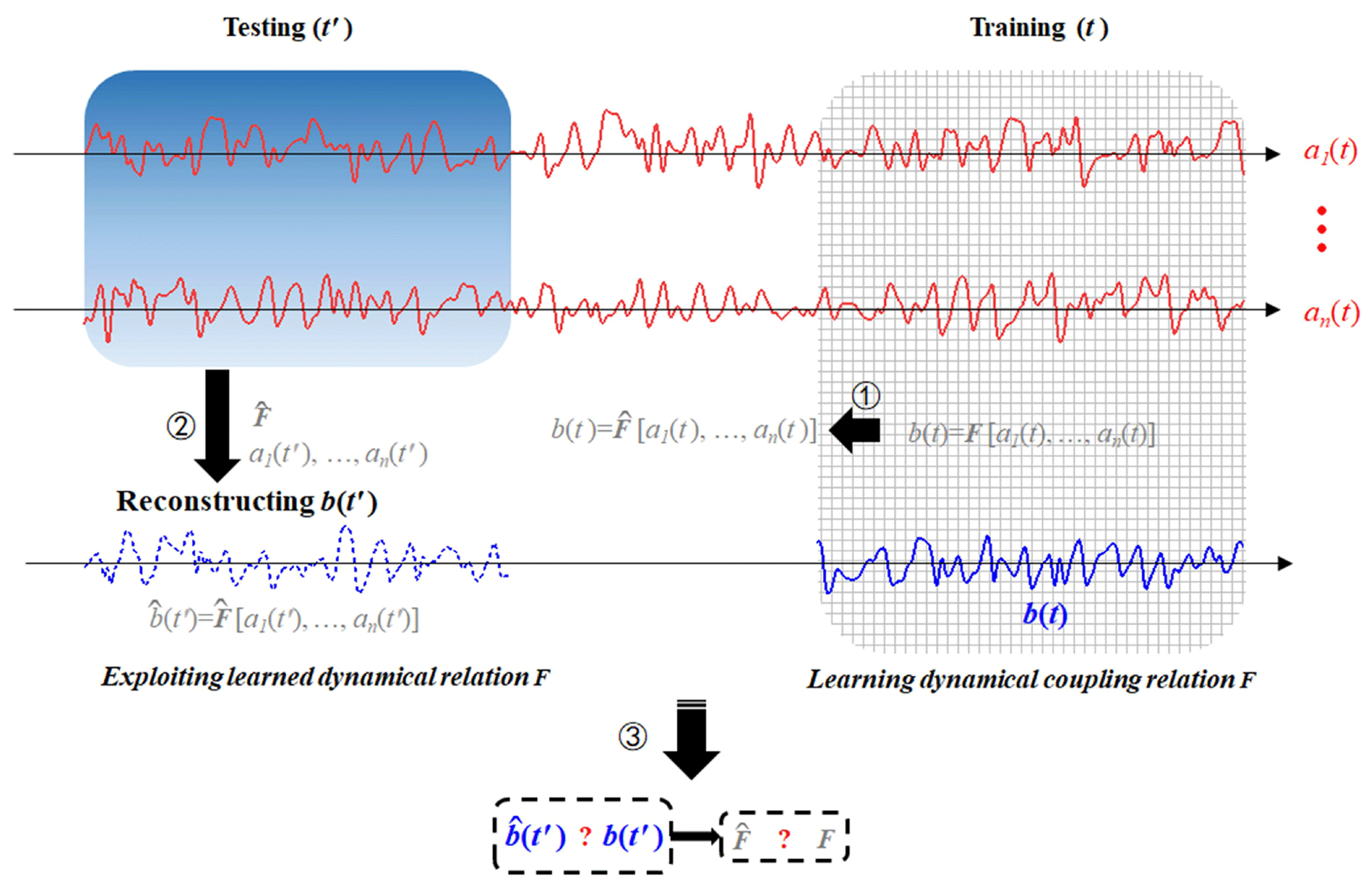
Figure 1 Diagram illustration for reconstructing time series by machine learning. (1) The available part of the dataset {a₁(t),  … ,  a_n(t), b(t)} is used to train the neural network. F denotes the inherent coupling relation function among the variables a₁,  … ,  a_n, and b; $\widehat{F}$ denotes the inferred coupling relation by neural network. (2) The dataset {a₁(t^′), a₂(t^′),  … ,  a_n(t^′)} is input into the trained neural network, and the unknown series, b(t^′), can be reconstructed, denoted as $\widehat{b}\left(t^{\prime }\right)$. (3) If $\widehat{b}\left(t^{\prime }\right)\approx b\left(t^{\prime }\right)$; then, the approximation $\widehat{F}\approx F$ can be derived, which indicates that the coupling relation is well reconstructed.

2.2 Machine-learning methods

2.2.1 Reservoir computer

A newly developed neural network called RC (Du et al., 2017; Lu et al., 2017; Pathak et al., 2018) has three layers: the input layer, the reservoir layer, and the output layer (see Fig. 2). If a(t) and b(t) denote two time series from a system, then the following steps can be taken to estimate b(t) from a(t).

• i

  a(t) (a vector with length L) is input into the input layer and reservoir layer. There are four components in these layers: the initial reservoir state r(t) (a vector with dimension N, representing the N neurons), the adjacent matrix M (size N×N) representing connectivity of the N neurons, the input-to-reservoir weight matrix W_in (size N×L), and the unit matrix E (size N×N), which is crucial for modulating the bias in the training process (Lu et al., 2018). The elements of M and W_in are randomly chosen from a uniform distribution in the interval [−1, 1], and we set N=1000 here. (We have tested that this choice yields good performance.) These components are employed to derive output as an updated reservoir state r^*(t):

  $$\begin{array}{}\text{(1)}& {\mathit{r}}^{*}\left(t\right)=\tanh [M\cdot r(t)+{\mathbf{W}}_{\mathrm{in}}\cdot a(t)+E].\end{array}$$
• ii

  r^*(t) then transfers to the output layer that consists of the reservoir-to-output matrix W_out. And r^*(t) will be used to estimate the value of $\widehat{b}\left(t\right)$ (see Eq. 2).

  $$\begin{array}{}\text{(2)}& \widehat{b}\left(t\right)={\mathbf{W}}_{\mathrm{out}}\cdot r^{*}\left(t\right)\end{array}$$

  The mathematical form of W_out is defined as

  $$\begin{array}{}\text{(3)}& {\mathbf{W}}_{\mathrm{out}}=\arg {\text{min}}_{{\mathbf{W}}_{\mathrm{out}}}∥{\mathbf{W}}_{\mathrm{out}}\cdot r^{*}\left(t\right)-b\left(t\right)∥+\mathit{\alpha }∥{\mathbf{W}}_{\mathrm{out}}∥,\end{array}$$

and it is a trainable matrix that fits the relation between r^*(t) and b(t) in the training process. ∥⋅ ∥ denotes the L₂ norm of a vector (L₂ represents the least square method) and α is the ridge regression coefficient, whose values are determined after the training.

After this reservoir neural network is trained, we can use it to estimate b(t), and the estimated value is noted as $\widehat{b}\left(t\right)$.

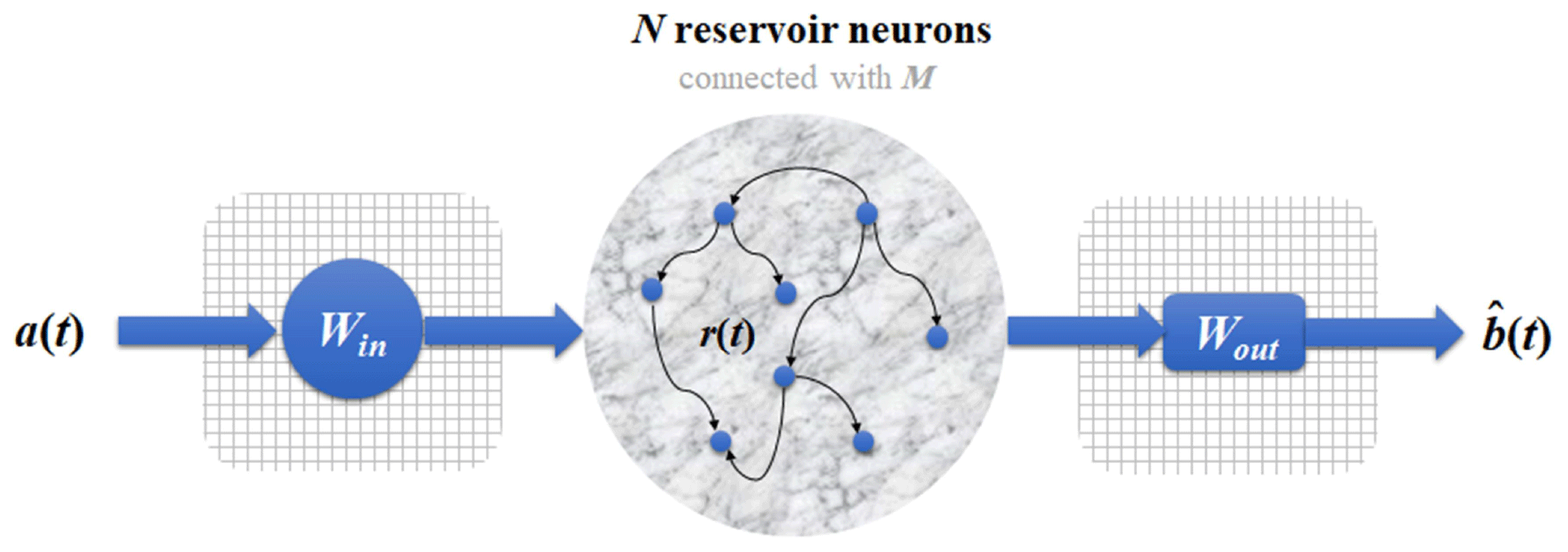
Figure 2 Schematic of the RC neural network: the three layers are the input layer, reservoir layer, and output layer. The input layer consists of a matrix W_in. The reservoir layer consists of N reservoir neurons whose connectivity is through the adjacent matrix M, and r(t) denotes the activation of neurons. The output layer consists of a matrix W_out; a(t) and $\widehat{b}\left(t\right)$ denote the input and output time series.

2.2.2 Backpropagation-based artificial neural network

Here, the used BP neural network is a traditional neural computing framework, and it has been widely used in climate research (Watson, 2019; Reichstein et al., 2019; Chattopadhyay et al., 2020). There are six layers in the BP neural network: the input layer has 8 neurons and four hidden layers with 100 neurons each; the output layer has 8 neurons. In each layer, the connectivity weights of the neurons need to be computed during the training process, where the backpropagation optimization with the complicated gradient decent algorithm is used (Dueben and Bauer, 2018). A crucial difference between the BP and the RC neural networks is as follows: unlike RC, all neuron states of the BP neural network are independent of the temporal variation of time series (Reichstein et al., 2019; Chattopadhyay et al., 2020), while the neurons of RC can track temporal evolution (such as the neuron state r(t) in Fig. 2) (Chattopadhyay et al., 2020). If a(t) and b(t) are two time series of a system, we can reconstruct b(t) from a(t) through the BP neural network.

2.2.3 Long short-term memory neural network

The LSTM neural network is an improved recurrent neural network to deal with time series (Reichstein et al., 2019; Chattopadhyay et al., 2020). As Fig. 3 shows, LSTM has a series of components: a memory cell, an input gate, an output gate, and a forget gate. When a time series a(t) is input to train this neural network, the information of a(t) will flow through all these components, and then the parameters at different components will be computed for fitting the relation between a(t) and b(t). The governing equations for the LSTM architecture are shown in the appendix. After the training is accomplished, a(t) can be used to reconstruct b(t) by this neural network.

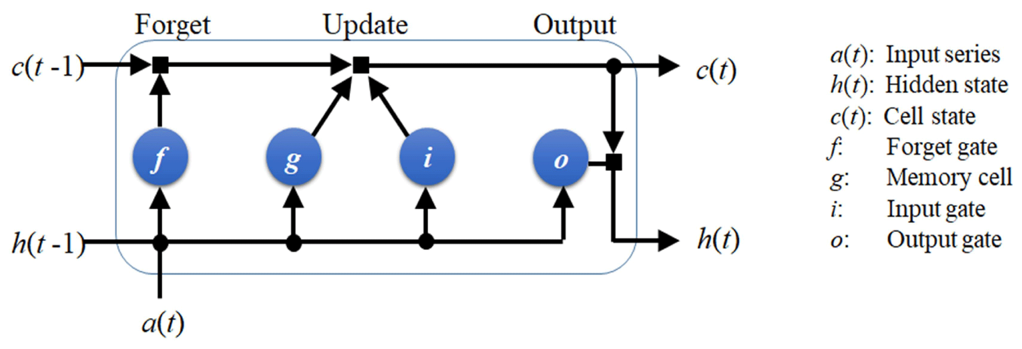
Figure 3 Schematic of the LSTM architecture. LSTM has a memory cell, an input gate, an output gate, and a forget gate to control the information of the previous time to flow into the neural network.

The crucial improvement of LSTM on the traditional recurrent neural network (Reichstein et al., 2019) is that LSTM has a forget gate which controls the information of the previous time to flow into the neural network. This will enable the neuron states of LSTM to track the temporal evolution of time series (Kratzert et al., 2019; Reichstein et al., 2019; Chattopadhyay et al., 2020), and this is the crucial difference between the LSTM and the BP neural networks.

Here, we also test the LSTM neural network without the forget gate and call it LSTM^*. This means that the information of the previous time cannot flow into the LSTM^* neural network, which does not have any memory of the past information. We will compare the performance of LSTM with that of LSTM^*, so the role of the neural network memory for the previous information can be presented.

2.3 Evaluation of reconstruction quality

The root-mean-square error (RMSE) of residuals is used here to evaluate the quality of reconstruction (Hyndman and Koehler, 2006). The residual represents the difference between the real series b(t^′) and the reconstructed series $\widehat{b}\left(t^{\prime }\right)$, and it is defined as

$$\begin{array}{}\text{(4)}& \text{RMSE}=\sqrt{{\displaystyle \frac{\mathrm{1}}{k}}\sum _t\left[b\right(t^{\prime })-\widehat{b}(t^{\prime }){]}^{\mathrm{2}}}.\end{array}$$

In order to fairly compare the errors of reconstructing different processes with different variability and units (Hyndman and Koehler, 2006; Pennekamp et al., 2019; Huang and Fu, 2019), we normalize the RMSE as

$$\begin{array}{}\text{(5)}& \text{nRMSE}={\displaystyle \frac{\text{RMSE}}{max\left[b\right(t^{\prime }\left)\right]-min\left[b\right(t^{\prime }\left)\right]}}.\end{array}$$

2.4 Coupling detection

2.4.1 Linear correlation

As mentioned in the introduction, the linear Pearson correlation is a commonly used method to quantify the linear relationship between two observational variables. The Pearson correlation between two series, a(t) and b(t), is defined as

$$\begin{array}{}\text{(6)}& \text{corr.}={\displaystyle \frac{\text{mean}\left[\right(a-\stackrel{\mathrm{‾}}{a})\cdot (b-\stackrel{\mathrm{‾}}{b}\left)\right]}{\text{SD}\left(a\right)\cdot \text{SD}\left(b\right)}}.\end{array}$$

The terms “mean” and “SD” denote the average and standard deviation for the series, respectively.

2.4.2 Convergent cross mapping

To measure the nonlinear coupling relation between two observational variables, we choose the convergent cross mapping (CCM) method that has been demonstrated to be useful for many complex nonlinear systems (Sugihara et al., 2012; Tsonis et al., 2018; Zhang et al., 2019). Considering a(t) and b(t) as two observational time series, we begin with the cross mapping (Sugihara et al., 2012) from a(t) to b(t) through the following steps:

• i

  Embedding a(t) (with length L) into the phase space is performed with a vector ${\mathit{M}}_a\left(t_i\right)=\mathit{\{}{a}_{t_i},a_{t_i-\mathit{\tau }},\mathrm{\dots },a_{t_i-(m-\mathrm{1})\mathit{\tau }}\mathit{\}}$ (t_i represents a historical moment in the observations), where embedding dimension (m) and time delay (τ) can be determined through the false nearest-neighbor algorithm (Hegger and Kantz, 1999).

• ii

  Estimating the weight parameter w_i denotes the associated weight between two vectors M_a(t) and M_a(t_i) (t denotes the excepted time in this cross mapping), and it is defined as

  $$\begin{array}{}\text{(7)}& {\displaystyle }{w}_i={\displaystyle \frac{u_i}{{\sum }_{i=\mathrm{1}}^{m+\mathrm{1}}{u}_i}},\text{(8)}& {\displaystyle }{u}_i=\exp {\displaystyle \frac{d\left[{\mathit{M}}_a\right(t),{\mathit{M}}_a(t_i\left)\right]}{d\left[{\mathit{M}}_a\right(t),{\mathit{M}}_a(t_{\mathrm{1}}\left)\right]}},\end{array}$$

  where d [M_a(t), M_a(t_i)] denotes the Euler distance between vectors M_a(t) and M_a(t_i). The nearest neighbor to M_a(t) generally corresponds to the largest weight.

• iii

  Cross mapping the value of b(t) is performed through

  $$\begin{array}{}\text{(9)}& \widehat{b}\left(t\right)={\sum }_{i=\mathrm{1}}^{m+\mathrm{1}}{w}_{i}b\left(t_i\right).\end{array}$$

  $\widehat{b}\left(t\right)$ denotes the estimated value of b(t) with this phase-space cross mapping. Then, we will evaluate the cross mapping skill (Sugihara et al., 2012; Tsonis et al., 2018) as:

  $$\begin{array}{}\text{(10)}& {\mathit{\rho }}_{a\to b}=\text{corr.}\left[b\right(t),\widehat{b}(t\left)\right].\end{array}$$

The cross mapping skill from b to a is also measured according to the above steps (marked as ρ_b→a). Sugihara et al. (2012) and Tsonis et al. (2018) defined the causal inference according to ρ_a→b and ρ_b→a as (i) if ρ_a→b is convergent when L is increased and ρ_a→b is of high magnitude, then b is suggested to be a causation of a. (ii) Besides, if ρ_b→a is also convergent when L is increased and is of high magnitude, then the causal relationship between a and b is bidirectional (a and b cause each other). In our study, all values of the CCM indices are measured when they are convergent with the data length (Tsonis et al., 2018).

According to previous studies (Sugihara et al., 2012; Ye et al., 2015), the CCM index is related to the ability of using one variable to reconstruct another variable: if b influences a but a does not influence b, the information content of b can be encoded in a (through the information transfer from b to a), but the information content of a is not encoded in b (there exists no information transfer from a to b). In this way, the time series of b can be reconstructed from the records of a. For the CCM index (ρ_a→b), its magnitude represents how much information content of b is encoded in the records of a. Therefore, the high magnitude of ρ_a→b means that b causes a, and we can get good reconstruction from a to b. In this paper, we will test the association between the CCM index and the reconstruction performance of machine learning.

3 Data

3.1 Time series from conceptual climate models

For a linearly coupled model, the autoregressive fractionally integrated moving average (ARFIMA) model (Granger and Joyeux, 1980) maps a Gaussian white noise ε(t) into a correlated sequence x(t) (Eq. 11), which can simulate the linear dynamics of an ocean–atmosphere coupled system (Hasselmann, 1976; Franzke, 2012; Massah and Kantz, 2016; Cox et al., 2018).

$$\begin{array}{}\text{(11)}& \mathit{\epsilon }\left(t\right)\stackrel{\text{ARFIMA}(p,d,q)}{⟶}x\left(t\right)\end{array}$$

In this model, d is a fractional differencing parameter, and p and q are the orders of the autoregressive and moving average components, respectively. Here, the parameters are set as p=3, d=0.2, and q=3. Hence x(t) is a time series composed of three components: the third-order autoregressive process whose coefficients are 0.6, 0.2, and 0.1; the fractional differencing process with Hurst exponent 0.7; and the third-order moving-average process whose coefficients are 0.3, 0.2, and 0.1 (Granger and Joyeux, 1980). These two time series, ε(t) and x(t), are used for the reconstruction analysis.

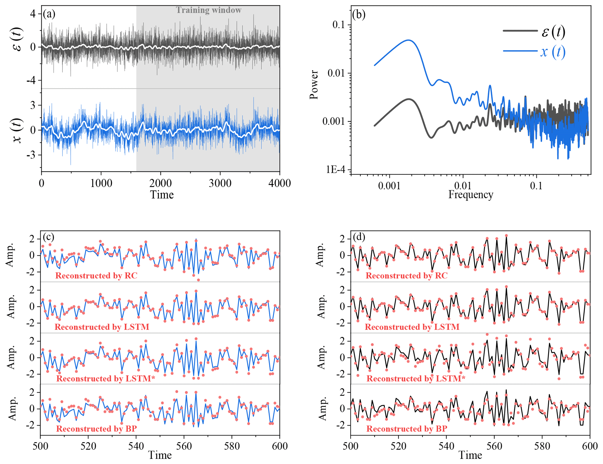
Figure 4 (a) The x(t) time series (blue) and the ε(t) time series (black) of the ARFIMA (3, 0.2,3) model. White lines denote the results of a 50-step running average. (b) Comparison of power spectra between x(t) and ε(t). (c) Comparison of the reconstructed time series of x(t) by RC, LSTM, LSTM^*, and BP (red dots), and blue lines denote the real x(t). (d) Comparison of the reconstructed time series of ε(t) through RC, LSTM, LSTM^*, and BP (red dots), and black lines denote the real ε(t).

For a nonlinearly coupled model, the Lorenz 63 chaotic system (Lorenz, 1963) depicts the nonlinear coupling relation in a low-dimensional chaotic system. The system reads as

$$\begin{array}{}\text{(12)}& \begin{array}{rl}& {\displaystyle \frac{\mathrm{d}x}{\mathrm{d}t}}=-\mathit{\sigma }(x-y),\\ & {\displaystyle \frac{\mathrm{d}y}{\mathrm{d}t}}=\mathit{\mu }x-xz-y,\\ & {\displaystyle \frac{\mathrm{d}z}{\mathrm{d}t}}=xy-Bz.\end{array}\end{array}$$

When the parameters are fixed at (σ, μ, B)= (10, 28, 8∕3), the state in the system is chaotic. We employed the fourth-order Runge–Kutta integrator to acquire the series output from this Lorenz 63 system. The time step was taken as 0.01. The time series X(t) and Z(t) are used for the reconstruction analysis.

For a high-dimensional model, the two-layer Lorenz 96 model (Lorenz, 1996) is a high-dimensional chaotic system, and it is commonly used to mimic midlatitude atmospheric dynamics (Chorin and Lu, 2015; Hu and Franzke, 2017; Vissio and Lucarini, 2018; Chen and Kalnay, 2019; Watson, 2019). It reads as

$$\begin{array}{}\text{(13)}& \begin{array}{rl}& {\displaystyle \frac{\mathrm{d}{X}_k}{\mathrm{d}t}}=X_{k-\mathrm{1}}(X_{k+\mathrm{1}}-X_{k-\mathrm{2}})-X_k+F-{\displaystyle \frac{h_{\mathrm{1}}}{J}}\sum _{j=\mathrm{1}}^J{Y}_{j,k},\\ & {\displaystyle \frac{\mathrm{d}{Y}_{k,j}}{\mathrm{d}t}}={\displaystyle \frac{\mathrm{1}}{\mathit{\theta }}}\left[Y_{k,j+\mathrm{1}}\right(Y_{k,j-\mathrm{1}}-Y_{k,j+\mathrm{2}})-Y_{k,j}+h_{\mathrm{2}}{X}_k].\end{array}\end{array}$$

In the first layer of the Lorenz 96 system, there are 18 variables marked as X_k (k is an integer ranging from 1 to 18), and each X_k is coupled with Y_k, j (Y_k, j is from the second layer). The parameters are set as fellows: J=20, h₁=1, h₂=1, and F=10. The parameter θ can alter the coupling strength: when θ is decreased, the coupling strength between X_k and Y_k, j will be enhanced. The fourth-order Runge–Kutta integrator and periodic boundary condition are adopted (i.e., X₀=X_K and $X_{K+\mathrm{1}}=X_{\mathrm{1}}$; $Y_{k,\mathrm{0}}=Y_{k-\mathrm{1},J}$ and $Y_{k,J+\mathrm{1}}=Y_{k+\mathrm{1},\mathrm{1}})$, and the integral time step is taken as 0.05. The time series X₁(t) and Y_1, 1(t) are used for the reconstruction analysis.

3.2 Real-world climatic time series

TSAT, NHSAT, and the Nino 3.4 index are chosen as the example from real-world climatic time series used for reconstruction analysis. The original data were obtained from the National Centers for Environmental Prediction (NCEP) (https://www.esrl.noaa.gov/psd/data/gridded/data.ncep.reanalysis2.html, last access: 16 September 2020) and KNMI Climate Explorer (http://climexp.knmi.nl, last access: 16 September 2020). The series of TSAT and NHSAT were obtained from the regional average of gridded daily data in NCEP Reanalysis 2. The selected spatial range is 20^∘ N–20^∘ S for the tropics and 20–90^∘ N for the Northern Hemisphere. The selected temporal range is from 1 September 1981 to 31 December 2018.

For the training and testing datasets before analysis, all the used time series are standardized to take zero mean and unit variance so that any possible impact of mean and variance on the statistical analysis is avoided (Brown, 1994; Hyndman and Koehler, 2006; Chattopadhyay et al., 2020). The total series were divided into two parts: 60 % of the time series for training the neural network and 40 % for the testing series. Specific data lengths of the training series and testing series will also be listed in the results section.

4 Results

4.1 Coupling relation learning

4.1.1 Linear coupling relation and machine learning

We first consider the simplest case: the linear coupling relation between two variables. Here, two time series x(t) and ε(t) in the ARFIMA (3, 0.2, 3) model are analyzed. Obviously, there are different temporal structures in x(t) and ε(t), especially for their large-scale trends (Fig. 4a) and power spectra (Fig. 4b). The marked difference between x(t) and ε(t) lies in their low-frequency variations, and there are more low-frequency and larger-scale structures in x(t) than in ε(t). We employ neural networks (RC, LSTM, LSTM^*, and BP) to learn the dynamics of this model (Eq. 11) through the procedure shown in Fig. 1. The training parts of ε(t) are selected from the gray shading in Fig. 4a. RC, LSTM, LSTM^*, and BP are trained to learn the coupling relation between x(t) and ε(t). Then, the trained neural networks together with ε(t) are used to reconstruct x(t). The reconstruction results and the performance of different neural networks are presented in Table 1. It shows that there is a strong linear correlation (0.88) between x(t) and ε(t). This reconstruction result suggests that the strong linear coupling can be well captured by these three neural networks since all values of nRMSE are low.

Table 1 Details of reconstructing ARFIMA (3, 0.2, 3).

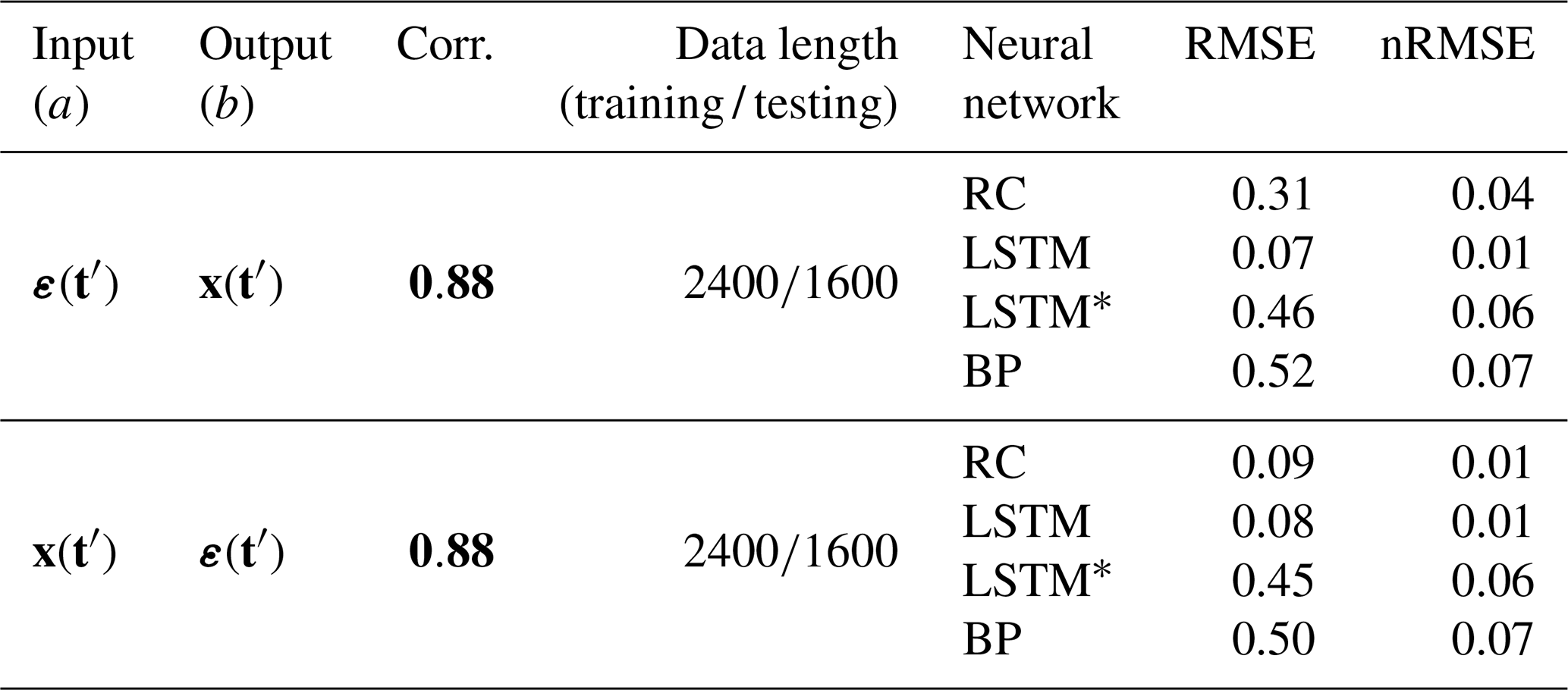
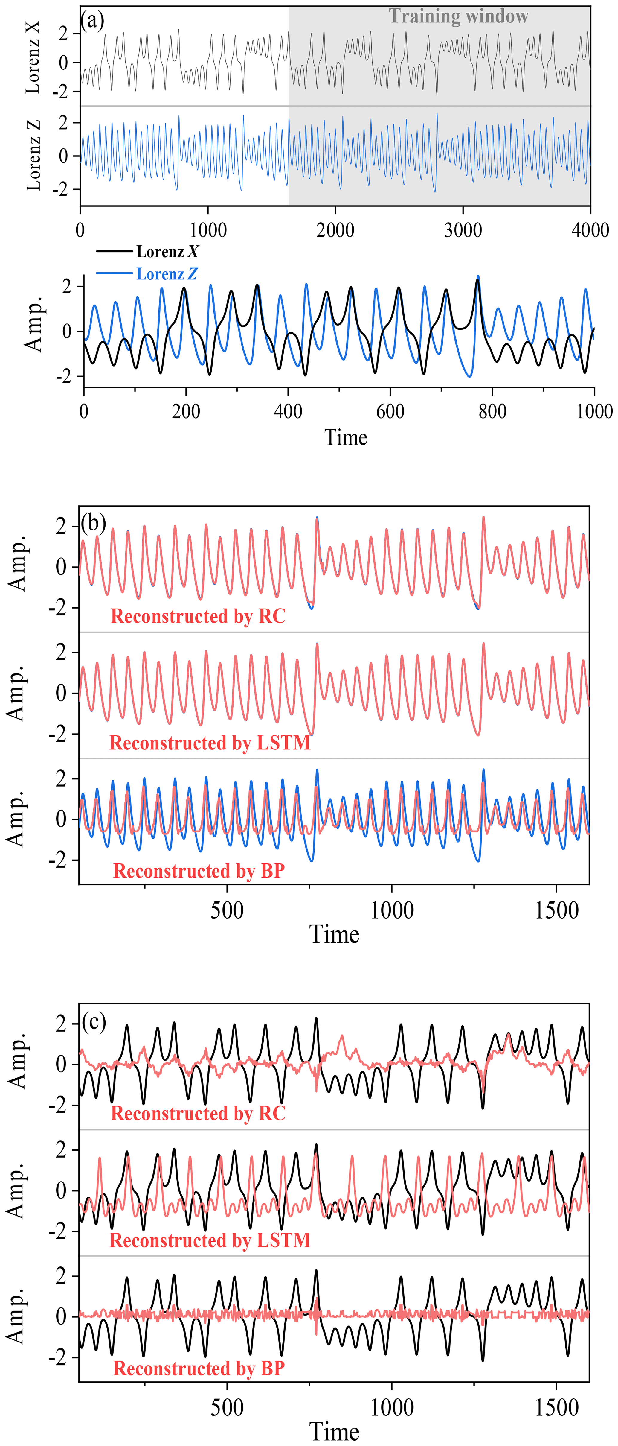
Figure 5 (a) The X time series (black) and the Z time series (blue) of the Lorenz 63 model. (b) Comparison of the reconstructed time series of Z (red) through RC, LSTM, and BP. Blue lines denote the real Z(t). (c) Comparison of the reconstructed time series of X(red) through RC, LSTM, and BP. Black lines are the real X(t).

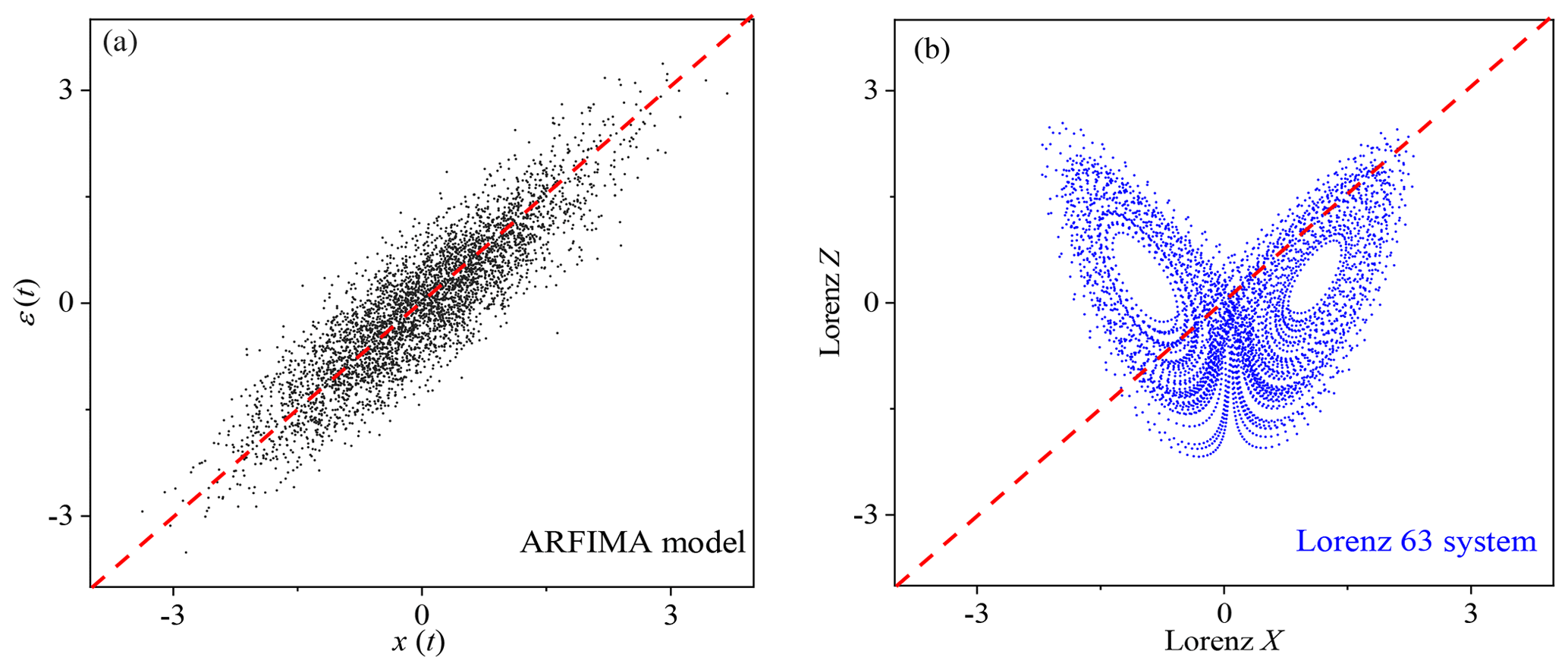
Figure 6 (a) Scatter plot of x(t) and ε(t) of the ARFIMA (3, 0.2, 3) model. (b) Scatter plot of X time series and Z time series of the Lorenz 63 model.

Detailed comparisons between the real and reconstructed series are shown in Fig. 4c and d. When ε(t) is input, the trained RC and LSTM neural networks can be applied to accurately reconstruct x(t). When x(t) is reconstructed from ε(t) through LSTM, the minimum of nRMSE (0.01) is reached; all reconstructed series are nearly overlapped with the real ones and cannot be visually differentiated (see Fig. 4c). For RC, the reconstruction quality is also good. The good performance of LSTM benefits from its memory function for the past information (Reichstein et al., 2019; Chattopadhyay et al., 2020). When the memory function of LSTM is stopped, the reconstruction of LSTM^* is no longer better than that of RC (see Table 1). The reconstruction by BP is successful in this linear system (Fig. 4), but its performance is not as good as LSTM and RC (Table 1). This performance difference may be due to the fact that, unlike LSTM and RC, the neuron states of BP cannot track the temporal evolution of a time series (Chattopadhyay et al., 2020).

4.1.2 Nonlinear coupling relation and machine learning

It is known that a strong linear correlation is useful for training neural networks and reconstructing time series. When the linear correlation between variables is very weak, could these machine-learning methods be applied to learn the underlying coupling dynamics? To address this question, two nonlinearly coupled time series, X(t) and Z(t), in the Lorenz 63 system (Lorenz, 1963) are analyzed.

There is a very weak overall linear correlation between variables X and Z (Pearson correlation: 0.002) in the Lorenz 63 model (Table 2), and such a weak linear correlation results from the time-varying local correlation between variables X and Z (see Fig. 5a). For example, X and Z are negatively correlated in the time interval of 0–200 but positively correlated in 200-400. This alternation of negative and positive correlation appears over the whole temporal evolutions of X(t) and Z(t), which leads to an overall weak linear correlation. In this case, we cannot use a feasible linear regression model between X(t) and Z(t) to reconstruct one from the other, since there is no such good linear dependency as found in the ARFIMA (p, d, q) system (see Fig. 6a and b).

Table 2 Details of Lorenz 63 system reconstruction.

Table 3 Details of reconstructing the Lorenz 96 model.

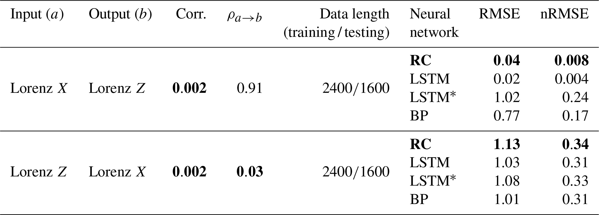
In a nonlinearly coupled system, it is known that the coupling strength between two variables cannot be estimated by the linear Pearson correlation (Brown, 1994; Sugihara et al., 2012). Here, we use CCM to estimate the coupling strength between X and Z, and it shows a high magnitude of the CCM index: ${\mathit{\rho }}_{X\to Z}=\mathrm{0.91}$. According to the CCM theory (see Methods section), such a high magnitude of the CCM index indicates that the information content of Z is encoded in the time series of X. Therefore, we conjecture that when inputting X(t) into the neural network, it is not only the information content of X(t) but also the information content of Z(t) that can be learned by the neural network. And then it is possible to reconstruct Z(t) from the trained neural network. We will test this in the following.

Figure 5b shows the results of reconstructing Z time series through RC, LSTM, and BP (upper, middle, and lower subpanels, respectively). Unlike the case of a linear system, the successful reconstruction for the time series of the Lorenz 63 system depends on the used machine-learning methods. The series reconstructed by LSTM nearly overlaps with the real series (Fig. 5b) and has the minimum nRMSE (0.004; see Table 2); moreover, the RC performs quite well, with only a little difference found at some peaks and dips (Fig. 5b). These reconstruction results suggest that even though the linear correlation is very weak, a strong nonlinear correlation will allow RC and LSTM to fully capture the underlying coupling dynamics. However, BP and LSTM^* perform poorly, and their reconstruction results have large errors (nRMSE =0.17 for BP, and nRMSE = 0.24 for LSTM^*). The reconstructed series heavily depart from the real series, especially for all peaks and dips, and the reconstructed values for each extreme point are underestimated (Fig. 5b). This means that both BP and LSTM^* cannot learn the nonlinear coupling.

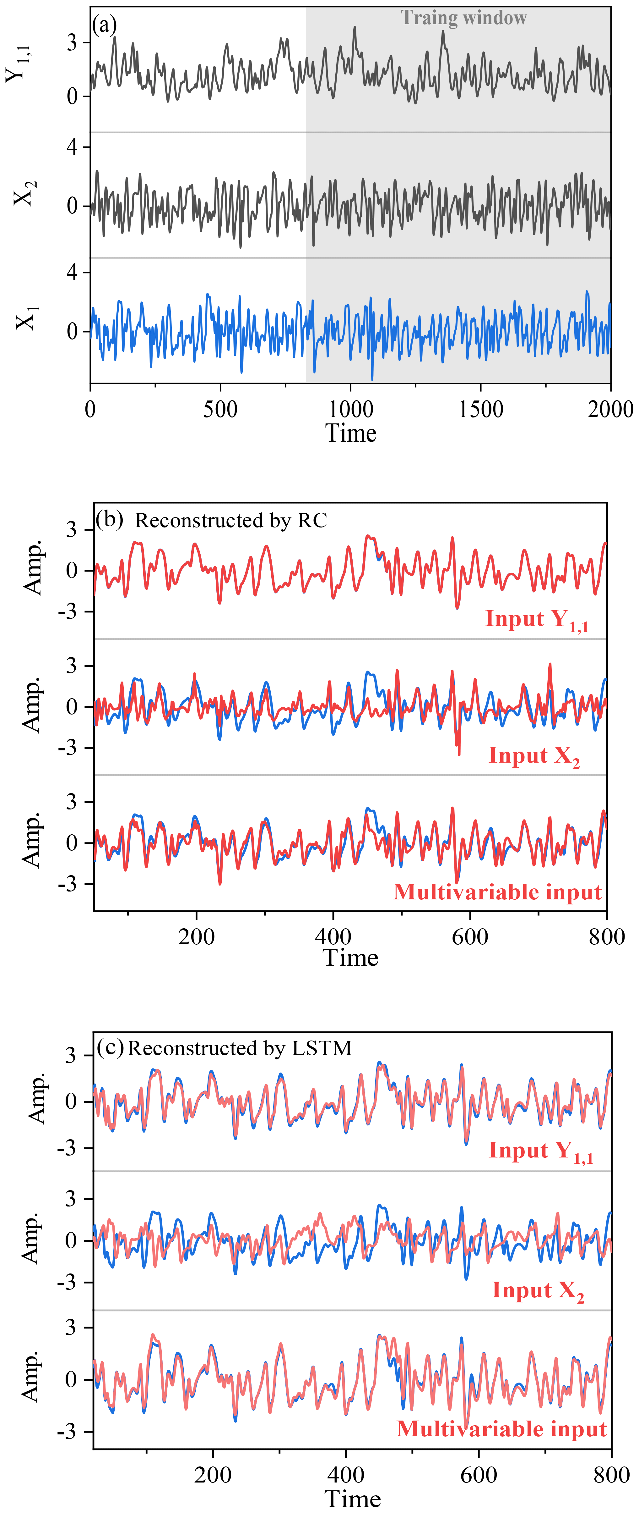
Figure 7 (a) The Y_1, 1 time series (black), X₂ time series (black), and X₁ time series (blue) of the Lorenz 96 system. (b) Reconstructed by RC; when Y_1, 1, X₂, and the multivariate are acting as the explanatory variables, the corresponding reconstructed X₁ time series (red) are shown, and blue lines denote the real X₁ time series. (c) Reconstructed by LSTM; when Y_1, 1, X₂, and the multivariate (multiple variables: X₂, X₁₇, and X₁₈) are acting as the explanatory variable, the corresponding reconstructed X₁ time series (red) are shown, and blue lines denote the real X₁ time series.

As mentioned in Sect. 2.2, a BP neural network does not track the temporal evolution, since its neuron states are independent of the temporal variation of time series. For LSTM^*, it does not include the information of previous time. Previous studies have revealed that the temporal evolution and memory are very important properties for a nonlinear time series (Kantz and Schreiber, 2004; Franzke et al., 2015), and this could not be neglected when modeling nonlinear dynamics. These might be responsible for the fact that BP and LSTM^* fail in dealing with this nonlinear Lorenz 63 system. Investigations for the application of BP in other nonlinear relationships need to be further addressed in the future.

4.2 Reconstruction quality and impact factors

From the above results, it is revealed that RC and LSTM are able to learn both linear and nonlinear coupling relations, and the coupled time series can be well reconstructed. In this section, we further investigate what factors can influence the reconstruction quality.

4.2.1 Direction dependence and variable dependence

When reconstructing time series of the linear model of Eq. (11), it can be found that the reconstruction is bidirectional (see Fig. 4d and Table 1): one variable can be taken as an explanatory variable to reconstruct another variable well; oppositely, it can also be well reconstructed by another variable. Furthermore, when the linear correlation is weak but the nonlinear coupling is strong, will the bidirectional reconstruction be still allowed? The answer is usually no! For example, when comparing the reconstruction quality of reconstructing Z(t) from X(t) (Fig. 5b) with that of reconstructing X(t) from Z(t) (Fig. 5c), all of the used machine-learning methods fail in reconstructing X(t) from Z(t) (large values of nRMSE are all close to 0.3). This result is consistent with the nonlinear observability mentioned by (Lu et al., 2017). The reconstruction direction is no longer bidirectional in this nonlinear system, but the reconstruction quality is direction dependent and variable dependent.

Therefore, we further discuss how to select the suitable explanatory variable or the reconstruction direction. Tables 1 and 2 show that the reconstruction quality in a linear coupled system highly depends on the Pearson correlation; however, it is different for a nonlinear system. For the Lorenz 63 system, the bidirectional CCM coefficients between the variables X and Z are asymmetric (with a stronger ${\mathit{\rho }}_{X\to Z}=\mathrm{0.91}$ but weaker ${\mathit{\rho }}_{Z\to X}=\mathrm{0.03})$; variable Z can be well reconstructed from variable X by machine learning, but X cannot be reconstructed from Z (Fig. 5b and c). The CCM index can be taken as a potential indicator to determine the explanatory variable and reconstructed variable for this nonlinear system. Here the asymmetric reconstruction quality results from the asymmetric information transfer between the two nonlinearly coupled variables (Hermann and Krener, 1977; Sugihara et al., 2012; Lu et al., 2017). In the coupling relation between X and Z, much more information content of Z is encoded in X, so it performs well for reconstructing Z from X (Lu et al., 2017), which can be detected by the CCM index (Sugihara et al., 2012; Tsonis et al., 2018).

4.2.2 Generalization to a high-dimensional chaotic system

Choosing direction and variable is important for the application of neural networks in reconstructing nonlinear time series, but this is derived from the low-dimensional Lorenz 63 system. In this subsection, we present the results from a high-dimensional chaotic system of the Lorenz 96 model. Furthermore, we will investigate the association between the CCM index and reconstruction quality in the machine-learning frameworks.

Firstly, we use variables X₁ and Y_1, 1 in Eq. (13) to illustrate the direction dependence in the high-dimensional system. Details of X₁ and Y_1, 1 are shown in Fig. 7a, and the Pearson correlation between X₁ and Y_1, 1 is weak (only −0.11; see Table 3). In Eq. (13), the forcing from X₁ to Y_1, 1 is much stronger than the forcing from Y_1, 1 to X₁. The CCM index shows: ${\mathit{\rho }}_{Y_{\mathrm{1},\mathrm{1}}\to X_{\mathrm{1}}}=\mathrm{0.98}$ and ${\mathit{\rho }}_{X_{\mathrm{1}}\to Y_{\mathrm{1},\mathrm{1}}}=\mathrm{0.61}$. This indicates that reconstructing X₁ from Y_1, 1 may obtain a better quality than from X₁ to Y_1, 1. As expected, by means of RC, the error of reconstructing X₁ from Y_1, 1 is nRMSE =0.01; however, it is nRMSE =0.06 in the opposite direction (Table 3). The result of LSTM is similar to that of RC in this case. Thus, direction dependence does exist in reconstructing this high-dimensional system, and the result is consistent with the indication of the CCM index. In this case, performance of the reconstruction through BP and LSTM^* is not good and the same as analyzed in Sect. 4.2.3.

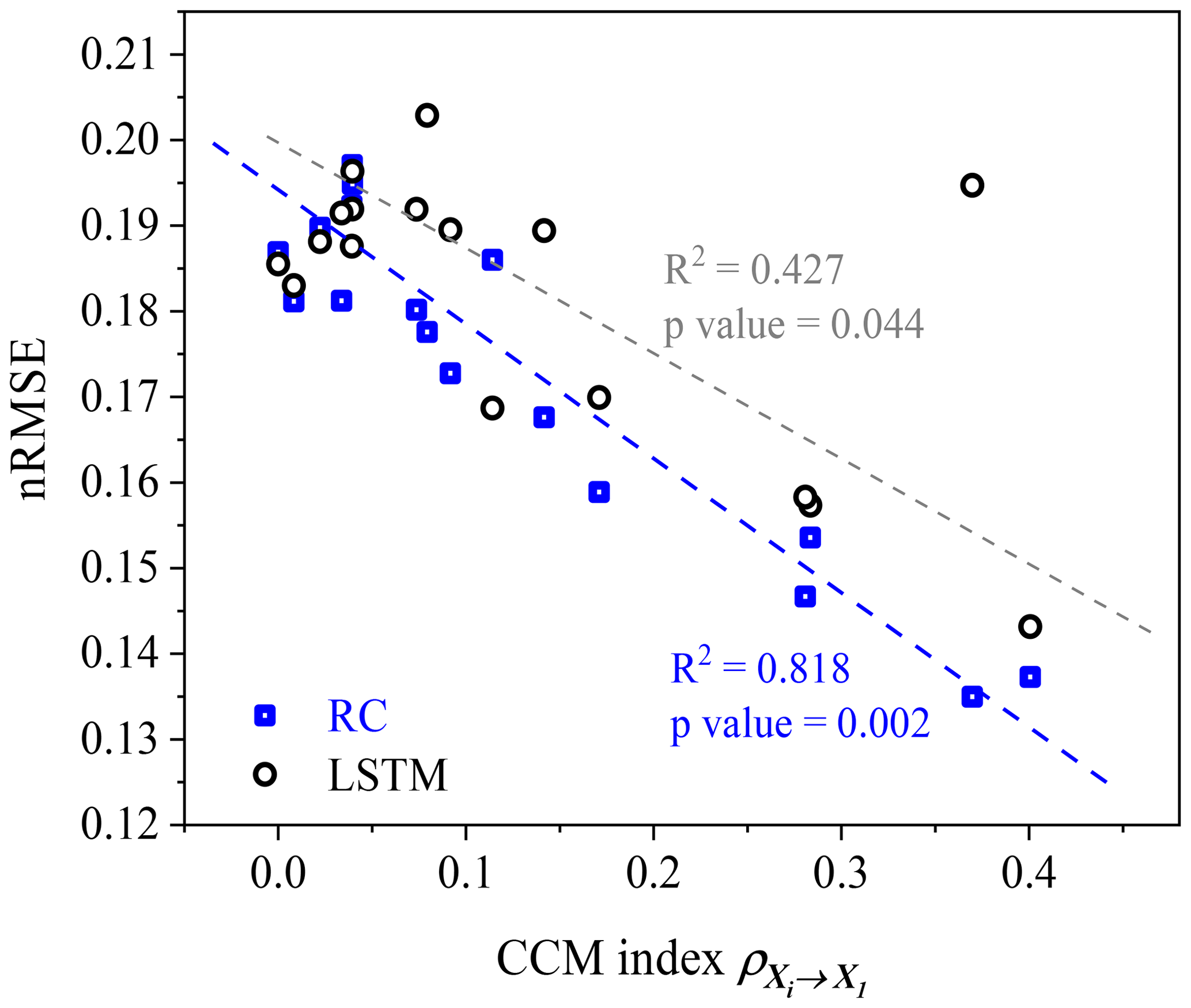
Figure 8 Scatter plot of nRMSE values and the CCM index values. Blue and gray dashed lines are the fitted linear trends for the scatters.

The reconstruction between X₁ and X₂ in the same layer of the Lorenz 96 system is also shown. There is an asymmetric causal relation (${\mathit{\rho }}_{X_{\mathrm{2}}\to X_{\mathrm{1}}}=\mathrm{0.37}$ and ${\mathit{\rho }}_{X_{\mathrm{1}}\to X_{\mathrm{2}}}=\mathrm{0.25})$ between X₁ and X₂, and their linear correlation is very weak (see Table 3). The RC gives a better result of reconstructing X₁ from X₂ (nRMSE =0.13) than reconstructing X₂ from X₁ (nRMSE =0.17). LSTM also has different results for the reconstructed X₁ and X₂ (Table 3), where the quality of reconstructing from X₁ to X₂ (nRMSE =0.16) is better than reconstructing from X₂ to X₁ (nRMSE =0.20). In this case, the reconstruction quality of LSTM is worse than that of RC, and the reconstruction results by LSTM are consistent with the indication of the CCM index. Chattopadhyay et al. (2020) also suggests that LSTM performs worse than RC in some cases, and this might be related to the use of a simple variant of the LSTM architecture. This variant of LSTM was tested and it was found that the time-varying local mean in time series would sometimes influence its performance. However, further investigation is required for a deeper understanding of the real reason. In this high-dimensional system, the reconstruction quality is also influenced by the chosen explanatory variables: the quality of reconstructing X₁ from Y_1, 1 is better than the quality of reconstructing X₁ from X₂ through RC and LSTM (see Fig. 7b and c).

Figure 9 Influence of strong nonlinear coupling on linear Pearson correlation and machine-learning performance. (a) Comparison of the linear correlation with different coupling strength. (b) Comparison of the machine-learning performance with different coupling strength. The black lines are the real series; the reconstructed series by RC (green lines), LSTM^* (blue lines), and BP (red dots) are shown. (Here the results of LSTM are overlapped with those of RC.)

Figure 10 (a) Daily time series of TSAT, NHSAT, and Nino 3.4 index. (b) Scatter plot of normalized NHSAT and normalized TSAT. (c) Three-dimensional scatter plot of normalized NHSAT, normalized TSAT, and normalized Nino 3.4 sea surface temperature.

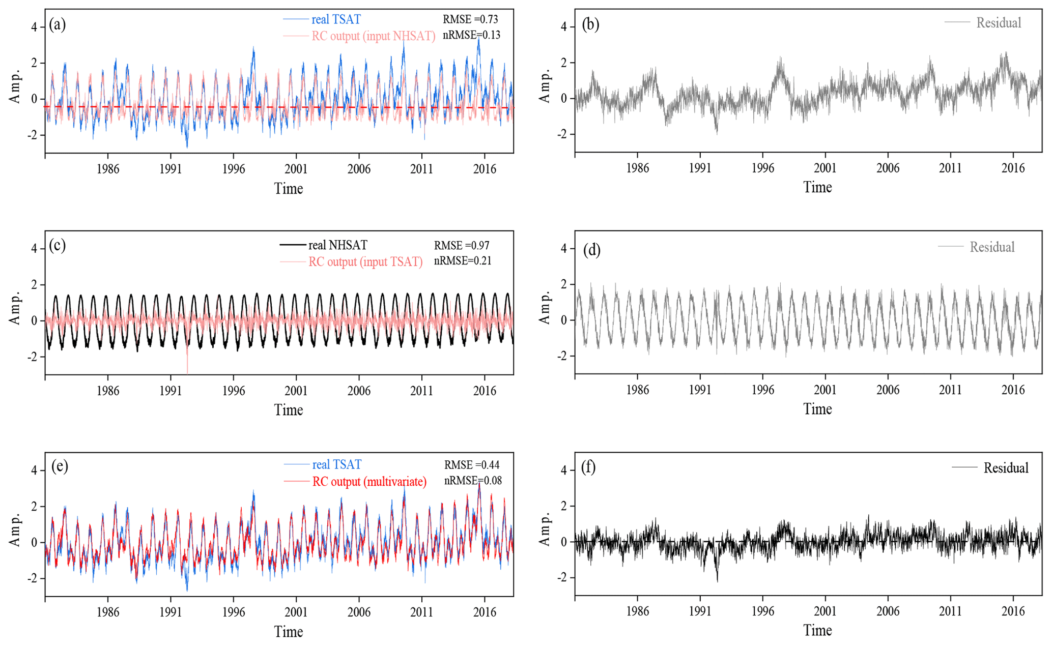
Figure 11 (a) Reconstructed TSAT time series from NHSAT, and its residual series (b); (c) reconstructed NHSAT time series from TSAT, and its residual series (d); (e) reconstructed TSAT time series from NHSAT and Nino 3.4 index, and its residual series (f).

Besides, the number of the chosen explanatory variables also influences the reconstruction quality. If more than one explanatory variable in the same layer is used, the reconstruction of X₁ from X₂ can be greatly improved (see Fig. 7b and c). For example, when all of X₂, X₁₇, and X₁₈ are acting as the explanatory variables, the nRMSE of reconstructed X₁ is reduced from 0.13 to 0.08 (Table 3). For both RC and LSTM, the multivariable reconstruction reaches lower error than those from unit-variable reconstruction.

In the above results, the CCM index is used to select explanatory variable for RC and LSTM. Now we employ more variables to test the association between the CCM index of the data and the performance of RC and LSTM. The values of the CCM index are calculated between X₁ and X₂, X₃, … , X₁₈; meanwhile, X₁ is reconstructed from X₂, X₃, … , X₁₈. We find a significant correspondence between the nRMSE and the CCM index (Fig. 8) for both RC and LSTM. Here we only use a simple LSTM architecture, and there are many other variants of this architecture where the abnormal point of LSTM in Fig. 8 might be reduced. The result of Fig. 8 reveals the robust association between the CCM index and reconstruction quality in the machine-learning frameworks of RC and LSTM. For other machine-learning methods, such association deserves further investigation.

4.2.3 Performance of BP and LSTM^* in the Lorenz 96 system

In nonlinear systems, the performance of reconstruction through BP and LSTM^* is much worse than that of RC and LSTM (Fig. 5). Here we present a simple experiment to illustrate what might influence the performance of BP and LSTM^* in a nonlinear system.

The experiment is set up as follows: in Eq. (13), the value of h₁ is set as 0, and the value of θ is decreased from 0.7 to 0.3. When θ is equal to 0.7, the forcing from X₁ to Y_1, 1 is weak (the Pearson correlation between X₁ and Y_1, 1 is only 0.48), and the performance values of BP and LSTM^* are not good. When θ is equal to 0.3, the forcing is dramatically magnified. As the second subpanel in Fig. 9a shows, the strong forcing makes Y_1, 1 synchronized to X₁, and the Pearson correlation between X₁ and Y_1, 1 is greatly increased to 0.8. When the forcing strength is magnified, the performance of machine learning is also enhanced (Fig. 9b): the reconstructed series by BP and the reconstructed series by LSTM^* are much closer to the real target series. This means that the reconstruction quality of BP and LSTM^* is greatly improved when the linear correlation is increased. This experiment reveals that the coupling strength in a nonlinear system can alter the Pearson correlation of the two time series, which further influences the performance of BP and LSTM^* in a nonlinear system.

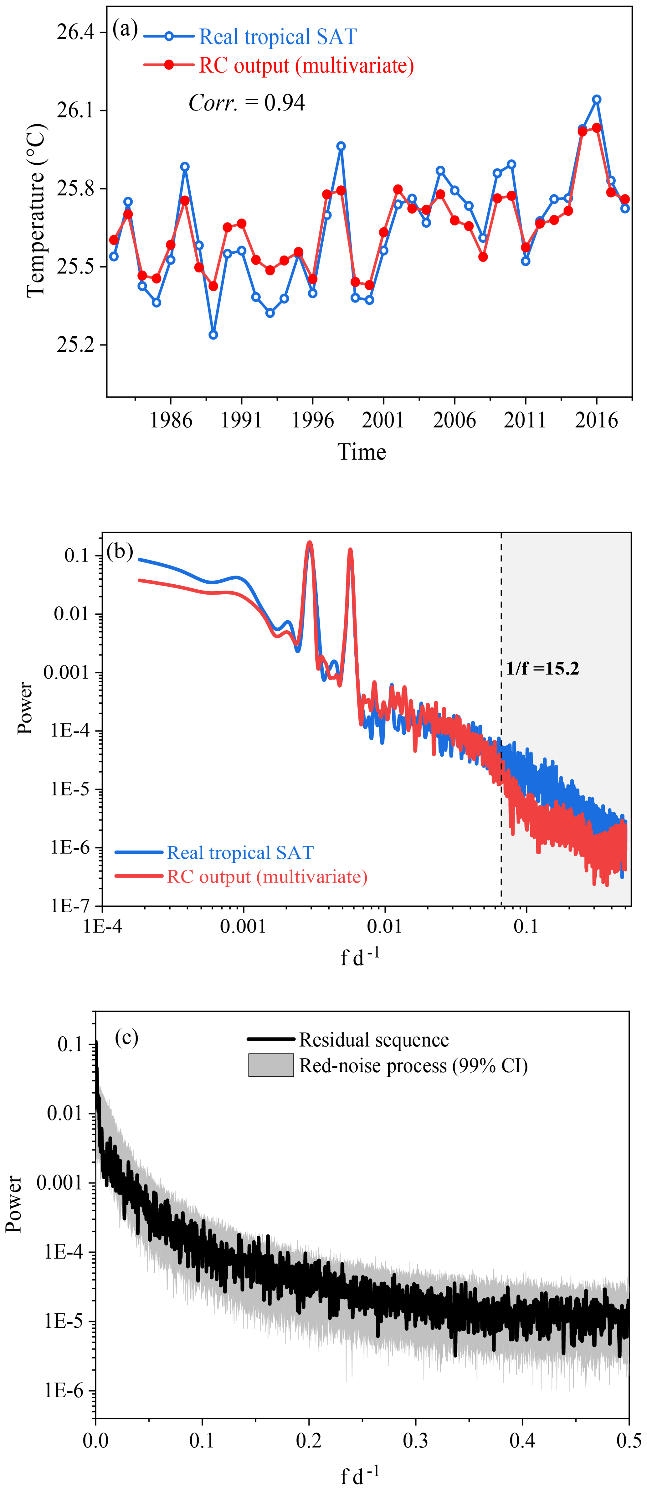
Figure 12 (a) Comparison of the annual mean values between the reconstructed TSAT and real TSAT. (b) Comparison of the power spectrum between the reconstructed TSAT and real TSAT. (c) A red-noise test for residual series.

Table 4 Details of the temperature record reconstruction.

However, RC and LSTM are not restricted to the Pearson correlation in this nonlinear system. When θ is altered from 0.7 to 0.3, although the Pearson correlation is changed a lot, the values of the CCM index are kept consistently above 0.9. For all values of θ, RC is able to equally produce a good-quality reconstruction of X₁. Figure 9b shows that the reconstructed series through RC and LSTM always overlap with the real time series. These results indicate that the performance of both RC and LSTM is sensitive to the value of CCM index, which is in line with the results given in Sect. 4.2.2.

4.3 Application to real-world climate series: reconstructing SAT

The natural climate series are usually nonstationary and are encoded with the information of many physical processes in the earth system. In the following, we illustrate the utility of the above methods and conclusions by investigating a real-world example.

The daily NHSAT and TSAT time series are shown in Fig. 10a. There are quite different temporal patterns in the NHSAT and TSAT series, with a weak linear correlation (0.08; see Table 4) between them. In the scatter plot for the NHSAT and TSAT (Fig. 10b), the marked nonlinear structure is observed between NHSAT and TSAT. Such a weak linear correlation will make the linear regression method fail to reconstruct one series from the other. Meanwhile, there is no explicit physical expression that can transform TSAT and NHSAT to each other. Now we try to use machine learning to learn their coupling between them and then to reconstruct these climate series. The CCM index when NHSAT cross maps TSAT is 0.70, and the CCM index when TSAT cross maps NHSAT is 0.24 (Table 4). The CCM index means that the information content of TSAT is well encoded in the records of NHSAT, and the information transfer might be mainly from TSAT to NHSAT. This finding is consistent with previous studies (Vallis and Farneti, 2009; Farneti and Vallis, 2013). Further, the CCM analysis indicates that the reconstruction from NHSAT to TSAT might obtain a better quality than that from the opposite direction.

The results validate our conjecture that the nRMSE of reconstruction from NHSAT to TSAT is lower than that from TSAT to NHSAT (Table 4). By using RC, the TSAT time series can be relatively well described by the reconstructed ones (Fig. 11a), with nRMSE equal to 0.13. This nRMSE is a bit high because some extremes of the TSAT time series have not been well described (Fig. 11b). When using TSAT to reconstruct the time series of NHSAT, the reconstructed time series cannot describe the real time series of NHSAT (Fig. 11c), and the corresponding nRMSE is equal to 0.21. Besides, we also use LSTM and BP to reconstruct these natural climate series; the performances of these two neural networks are worse than RC (Table 4). For BP, this worse performance may be due to its inability to deal with nonlinear coupling. LSTM performs worse than RC in this real-world case, which might be induced by the used simple variant of LSTM architecture.

We can further improve the reconstruction quality of TSAT. Considering that the tropical climate system interacts not just with the Northern Hemisphere climate system, we can use the information of other systems to improve the reconstruction. Looking at the time series of the Nino 3.4 index (Fig. 10a), some of its extremes occur at the same time intervals as the extremes of TSAT. Moreover, when the Nino 3.4 index is included in the scatter plot (Fig. 10c), a nonlinear attractor structure is revealed. We combine NHSAT with the Nino 3.4 index to reconstruct the time series of TSAT through RC. The reconstructed TSAT (Fig. 11e) is much closer to the real TSAT series, and the corresponding nRMSE has been reduced to 0.08.

Finally, we make a further comparison between the real TSAT and the reconstructed TSAT. (i) The annual variations of the reconstructed TSAT are close to those of the real TSAT (Fig. 12a). (ii) The power spectra of TSAT and the reconstructed TSAT are compared in Fig. 12b, and the main deviation occurs at the frequency bands of 0–15 d. The reason might be that the local weather processes are not input into this RC reconstruction. This conjecture can be further confirmed through a red-noise test with response time of 15 d for the residual series (this red-noise test is the same as the method used in Roe, 2009). All data points of the residual series lie within the confidence intervals (Fig. 12c). This means that the residual is possibly induced by local weather processes, and this information is not input into RC for the reconstruction.

5 Conclusions and discussions

In this study, three kinds of machine-learning methods are used to reconstruct the time series of toy models and real-world climate systems. One series can be reconstructed from the other series by machine learning when they are governed by the common coupling relation. For the linear system, variables are coupled through the linear mechanism, and a large Pearson coefficient can benefit machine learning with bidirectional reconstruction. For a nonlinear system, the coupled time series often have a small Pearson coefficient, but machine learning can still reconstruct the time series when the CCM index is strong; moreover, the reconstruction quality is direction dependent and variable dependent, which is determined by the coupling strength and causality between the dynamical variables.

Choosing suitable explanatory variables is crucial for obtaining a good reconstruction quality. But the results show that machine-learning performance cannot be explained only by the linear correlation. In this study, we suggest to use the CCM index to select explanatory variables. Especially for the time series of nonlinear systems, the strong CCM index can be taken as a benchmark to select an explanatory variable. When the CCM index is higher than 0.5 in this study, the nRMSE is often smaller than 0.1, with the reconstructed series very close to the real series in the presented results. Thus, the CCM index higher than 0.5 may be considered a criterion for choosing appropriate explanatory variables. It is well known that atmospheric or oceanic motions are nonlinearly coupled over most timescales; therefore, in the natural climate series, there would be similar nonlinear coupling relations as found in the Lorenz 63 and the Lorenz 96 systems (weak Pearson correlation but high CCM coefficient). If only Pearson coefficient is used to select the explanatory variable, then some useful nonlinearly correlated variables may be left out.

Finally, it is worth noting the potential application for machine learning in climate studies. For instance, when a series b(t) is unmeasured during some period because of measuring instrument failure but there are other kinds of variables without missing observations, then CCM can be applied to select the suitable variables coupled with b(t), and RC or LSTM can be employed to reconstruct the unmeasured part of b(t) (following Fig. 1). This is useful for some climate studies, such as paleoclimate reconstruction (Brown, 1994; Donner 2012; Emile-Geay and Tingley, 2016), interpolation of the missing points in measurements (Hofstra et al., 2008), and parameterization schemes (Wilks, 2005; Vissio and Lucarini, 2018). Our study in this article is only a beginning for reconstructing climate series by machine learning, and more detailed investigations will be reported soon.

Appendix A: Governing equations for the LSTM neural network

If a(t) and b(t) denote two time series and a(t) is input into LSTM to estimate b(t), then the governing equations for the LSTM architecture (Fig. 3) are as follows:

$$\begin{array}{}\text{(A1)}& {\displaystyle }f\left(t\right)={\mathit{\sigma }}_f\left(W_f\left[h\left(t-\mathrm{1}\right),a\left(t\right)\right]+s_f\right),\text{(A2)}& {\displaystyle }i\left(t\right)={\mathit{\sigma }}_f\left(W_i\left[h\left(t-\mathrm{1}\right),a\left(t\right)\right]+s_i\right),\text{(A3)}& {\displaystyle }\stackrel{\mathrm{̃}}{c}\left(t\right)=\tanh \left(W_c\left[h\left(t-\mathrm{1}\right),a\left(t\right)\right]+s_h\right),\text{(A4)}& {\displaystyle }c\left(t\right)=f\left(t\right)c\left(t-\mathrm{1}\right)+i\left(t\right)\stackrel{\mathrm{̃}}{c}\left(t\right),\text{(A5)}& {\displaystyle }o\left(t\right)={\mathit{\sigma }}_h(W_h\left[h\left(t-\mathrm{1}\right),a\left(t\right)\right]+s_h),\text{(A6)}& {\displaystyle }h\left(t\right)=o\left(t\right)\tanh \left(c\right(t\left)\right),\text{(A7)}& {\displaystyle }\widehat{b}\left(t\right)=W_{oh}h\left(t\right).\end{array}$$

f(t), i(t), and o(t) denote the forget gate, input gate, and output gate, respectively. h(t) and c(t) represent the hidden state and the cell state, respectively; the dimension of the hidden layers is set as 200, which could yield the good performance in our experiment. All these components can be found in Fig. 3, and the information flow among these components are realized by Eqs. (14)–(20). There are many parameters in the LSTM architecture: σ_f is the softmax activation function; s_f, s_i, and s_h are the biases in the forget gate, the input gate, and the hidden layers, respectively; the weight matrixes W_f, W_i, W_c, and W_oh denote the neuron connectivity in each layer. These parameters need to be computed during training (Chattopadhyay et al., 2020); a(t) and $\widehat{b}\left(t\right)$ represent the input and output time series.