the Creative Commons Attribution 4.0 License.
the Creative Commons Attribution 4.0 License.
 | 16 Dec 2020
Future sea level contribution from Antarctica inferred from CMIP5 model forcing and its dependence on precipitation ansatz
Christian B. Rodehacke
Madlene Pfeiffer
Tido Semmler
Özgür Gurses
Thomas Kleiner
Various observational estimates indicate growing mass loss at Antarctica's margins as well as heavier precipitation across the continent. Simulated future projections reveal that heavier precipitation, falling on Antarctica, may counteract amplified iceberg discharge and increased basal melting of floating ice shelves driven by a warming ocean. Here, we test how the ansatz (implementation in a mathematical framework) of the precipitation boundary condition shapes Antarctica's sea level contribution in an ensemble of ice sheet simulations. We test two precipitation conditions: we either apply the precipitation anomalies from CMIP5 models directly or scale the precipitation by the air temperature anomalies from the CMIP5 models. In the scaling approach, it is common to use a relative precipitation increment per degree warming as an invariant scaling constant. We use future climate projections from nine CMIP5 models, ranging from strong mitigation efforts to business-as-usual scenarios, to perform simulations from 1850 to 5000. We take advantage of individual climate projections by exploiting their full temporal and spatial structure. The CMIP5 projections beyond 2100 are prolonged with reiterated forcing that includes decadal variability; hence, our study may underestimate ice loss after 2100. In contrast to various former studies that apply an evolving temporal forcing that is spatially averaged across the entire Antarctic Ice Sheet, our simulations consider the spatial structure in the forcing stemming from various climate patterns. This fundamental difference reproduces regions of decreasing precipitation despite general warming. Regardless of the boundary and forcing conditions applied, our ensemble study suggests that some areas, such as the glaciers from the West Antarctic Ice Sheet draining into the Amundsen Sea, will lose ice in the future. In general, the simulated ice sheet thickness grows along the coast, where incoming storms deliver topographically controlled precipitation. In this region, the ice thickness differences are largest between the applied precipitation methods. On average, Antarctica shrinks for all future scenarios if the air temperature anomalies scale the precipitation. In contrast, Antarctica gains mass in our simulations if we apply the simulated precipitation anomalies directly. The analysis reveals that the mean scaling inferred from climate models is larger than the commonly used values deduced from ice cores; moreover, it varies spatially: the highest scaling is across the East Antarctic Ice Sheet, and the lowest scaling is around the Siple Coast, east of the Ross Ice Shelf. The discrepancies in response to both precipitation ansatzes illustrate the principal uncertainty in projections of Antarctica's sea level contribution.
- Article
(22655 KB) - Full-text XML
- BibTeX
- EndNote


Sea level rise as a symptom of progressive climate warming is of paramount importance for coastal societies, because it impacts numerous economic activities globally and threatens the population along coasts. An ice sheet's contribution to the future sea level is projected using statistical approaches that take advantage of deduced past behavior (Church et al., 2013a) or process-based model simulations, e.g., ice sheet models (Goelzer et al., 2018; Seroussi et al., 2019a). Adequate forcing fields are required to perform ice sheet model simulations covering centuries to glacial–interglacial (100 000-year) periods (e.g., Golledge et al., 2015; Winkelmann et al., 2012; Pollard and DeConto, 2009). These forcing fields are either descriptions based on linear multiple regression analysis (e.g., surface elevation and latitude dependence; Fortuin and Oerlemans, 1990) or originate from regional climate models or climatological data sets.
It is common for climate change experiments to deduce simplified forcing anomalies across selected climate scenarios (e.g., from CMIP models). As a further simplification step, the anomalies forced through time are often spatially homogeneous in these experiments. For example, a spatially homogeneous air temperature anomaly is applied across the entire Antarctic Ice Sheet on top of a background field representing the presently observed state. Compared with air temperature, the evolution of precipitation is more uncertain in both observational records (Hartmann et al., 2013) and models (Flato et al., 2013). Therefore, the precipitation forcing anomalies are commonly developed from the temperature forcing anomalies by prescribing a percentage increase in precipitation with temperature increase. The motivation behind this is the Clausius–Clapeyron process, where the saturation pressure of water vapor scales exponentially by about 7 % K−1 warming (Held and Soden, 2006) – it is implicitly assumed that the relative humidity does not change.
However, when considered globally, this rate – hereafter referred to as mean precipitation scaling – is less than the theoretical value deduced from thermodynamic principles. Climate modeling studies representing the Last Glacial Maximum (LGM), the preindustrial (piControl), and the historical period as well as climate warming scenarios (1pctCO2 and abrupt4xCO2) show that the global precipitation increases in warmer climates and decreases in colder climates at a rate between 1 % K−1 and 4 % K−1 (Held and Soden, 2006; Li et al., 2013).
Decreasing precipitation rates with global warming in the dry subtropics (Sun et al., 2007), covering a substantial part of the globe, expose a limitation of this scaling. They indicate that the assumption of a homogeneous increase in precipitation with global warming is not expected; for instance, future simulations of the 21st century show that the scaling in the Arctic of 4.5 % K−1 is much larger than the global value of 1.6 % K−1–1.9 % K−1 because retreating sea ice amplifies the hydrological cycle in the Arctic (Bintanja and Selten, 2014).
Both dynamical and thermodynamical processes contribute to the actual precipitation change, even if dynamical changes, such as changing circulation, play a secondary role globally (Emori and Brown, 2005). The balance of radiative fluxes in and out of the troposphere and the latent energy flux at the surface limits evaporation, which restricts water vapor supply regionally and, therefore, limits the scaling (Allen and Ingram, 2002).
A global analysis of observed precipitation and air temperature changes reveals a low or even negative scaling in tropical land regions driven by decreasing soil moisture, a near Clausius–Clapeyron scaling of ≈7 % K−1 over the open ocean, and a super Clausius–Clapeyron scaling of >7 % K−1 along extra-tropical coasts (Yin et al., 2018). In the latter case, the moisture supply from the ocean in concert with the atmospheric circulation generates extreme precipitation events inland. These events cause a high temperature scaling factor for precipitation onshore. Ultimately, the local availability and recycling of moisture and the atmospheric dynamics determine the size of the precipitation–temperature scaling (Yin et al., 2018). As the interplay between thermodynamic and atmospheric dynamics governs the scaling, it is unlikely that this scaling can be represented by a single value across Antarctica.
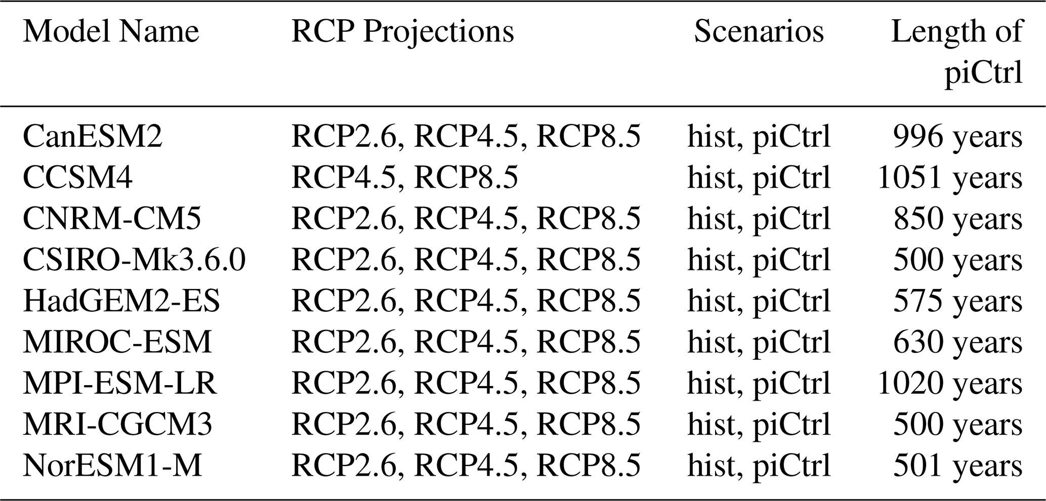
To overcome some of the limitations of forcing strategies of ice sheet models in previous studies, we exploit the full temporal and spatial pattern of the atmospheric and oceanographic forcing anomalies from CMIP5 models to perform transient simulations; this approach is unprecedented. We use the historical climate scenario (1850–2004) followed by three future Representative Concentration Pathway (RCP) climate scenarios (RCP2.6, RCP4.5, and RCP8.5; 2005–2100) from a compilation of nine CMIP5 models (Table 1) to drive numerous simulations with the Parallel Ice Sheet Model (PISM, e.g., Bueler and Brown, 2009; Winkelmann et al., 2011) for each climate projection. We compare these ice sheet simulations, considering the spatial inhomogeneities in transient climate forcing, with more traditional simulations in which the precipitation forcing anomaly is scaled with the temperature forcing anomaly.
Table 1List of the CMIP5 models and the RCP climate projections used, which cover the period from 2005 to 2100 (Moss et al., 2010) in addition to the historical scenario (“hist”, period from 1850 to 2004) and the piControl scenario (“piCtrl”). The fourth column lists the length of the piControl simulation. Note that we do not use the RCP2.6 scenario of the CCSM4 model. See also Table 3.
The following subsections provide an overview of observed and simulated precipitation changes (Sect. 1.1) over Antarctica from previous studies (Sect. 1.2). A description of factors influencing the precipitation and its scaling in Antarctica is then given. Afterward, Sect. 1.3 highlights processes that control Antarctica's mass balance.
1.1 Processes linked to precipitation scaling
While both the local availability and recycling of moisture and the atmospheric dynamics determine the size of the precipitation–temperature scaling in most regions (Yin et al., 2018), atmospheric dynamics dominate over the deep-frozen interior of the Antarctic continent, probably due to the negligible water buffering capacity of the frozen ground. The ocean surface conditions around Antarctica set the lower boundary condition for the atmosphere, which accounts for the spread of the precipitation scaling among climate models. Atmosphere simulations over Antarctica, which are driven by boundary conditions from a small ensemble of historical and future climate scenarios, show a weak impact of changed atmospheric conditions or enhanced radiative forcing on the scaling factor (Krinner et al., 2014). In contrast, the ocean conditions are crucial for the precipitation scaling in Antarctica (Krinner et al., 2014), because these conditions shape the atmospheric circulation, thereby determining the moisture flux that maintains the precipitation (Wang et al., 2020). Bracegirdle et al. (2015) showed that sea ice cover has a decisive impact and that the mean historical sea ice concentration is more important than the sea ice retreat rate.
Across Antarctica, the patterns of increasing and decreasing precipitation are consistent with the variability of the large-scale moisture transport resembling the known Southern hemispheric modes of variability, such as the Amundsen Sea low (ASL) or the Southern Annular Mode (SAM) (Fyke et al., 2017). Furthermore, the baroclinic annular mode (BAM) and the two Pacific–South American teleconnection (PSA1 and PSA2) indices influence precipitation over Antarctica (Marshall et al., 2017). An enhanced baroclinic annular mode, which corresponds to high storm amplitudes, increases precipitation over the coastal East Antarctic Ice Sheet, whereas an enhanced SAM causes stronger precipitation across the West Antarctic Ice Sheet (WAIS) and the neighboring Antarctic Peninsula. The two Pacific–South American teleconnections mainly impact precipitation over the West Antarctic Ice Sheet in addition to other regions across the Antarctic continent.
In reanalysis products, no robust or statistically significant precipitation trend exists over Antarctica (Bromwich et al., 2011). This result is in agreement with precipitation observations over the Southern Ocean (Bromwich et al., 2011). However, shallow ice cores across Antarctica reveal a tendency towards a positive precipitation trend over the last 50 years and 100 years. Since 1800, the increase in the surface mass balance (SMB) is estimated to be 7±1.3 Gt per decade (Thomas et al., 2017).
In contrast, over the western region of the West Antarctic Ice Sheet (WAIS), next to the Ross Ice Shelf, a negative snow accumulation trend has been detected in monthly reanalysis products (ERA-Interim: 1979–2010; ERA-20C: 1900–2010), which has been confirmed by a composite of 17 firn cores (Wang et al., 2017). The flow of available atmospheric moisture, which feeds the precipitation across the WAIS, is dominated by the Amundsen Sea low (Thomas et al., 2017). A location shift of the Amundsen Sea low (ASL), expressed by its longitudinal position, exposes different regions to the circulation branch of moisture-rich air masses that is directed inland – on the eastern side of the low's center – or isolates them from moisture supply due to the circulation branch that is directed offshore – on the western side of the low's center. Furthermore, the deepening of the ASL enhances the cyclonic circulation, which strengthens precipitation – southeast of the low's center – over the Antarctic Peninsula and eastern WAIS. However, fewer moisture-rich air masses reach the western WAIS, which ultimately leads to an accumulation deficit. An enlarged sea ice extent in the Ross Sea (Haumann et al., 2016; Liu, 2004) damps evaporation to the atmosphere. In contrast, a decreasing sea ice trend in the Amundsen and Bellingshausen seas (Haumann et al., 2016; Jacobs, 2006) enhances the moisture supply. To conclude, across the West Antarctic Ice Sheet, the observed accumulation reduction is driven by the deepening of the ASL and is further reinforced by a more extensive sea ice extent in the Ross Sea (Wang et al., 2017).
1.2 Scaling between precipitation and air temperature changes over Antarctica
In Antarctica (Fig. 1), global model simulations until the end of the century show an average scaling of about 7.4 % K−1 (range from 5.5 % K−1 to 24.5 % K−1, Palerme et al., 2017), which is in agreement with CloudSat estimates (7.1 % K−1 for the years 2007 to 2010; Palerme et al., 2017). For the last deglaciation, global climate models suggest a value of about 6 % K−1 in Antarctica, whereas future projections of a high-resolution regional climate model show a lower value of 4.9 % K−1 in contrast to a value of 6.1±2.6 % K−1 from an ensemble of global climate system models (Frieler et al., 2015) – which is similar to the value from global climate models for the last deglaciation. Ice core data covering 10 000 years of marked temperature changes reveal a value of 5±1 % K−1 (Frieler et al., 2015). In stand-alone ice sheet modeling studies, the commonly used temperature scaling factor for precipitation amounts to approximately 5 % K−1 (e.g., Gregory and Huybrechts, 2006) in Antarctica, as the latitudinal relation obtained from a CMIP5 model ensemble suggests (Golledge et al., 2015). We consider 5 % K−1 as the reference value from this point on.
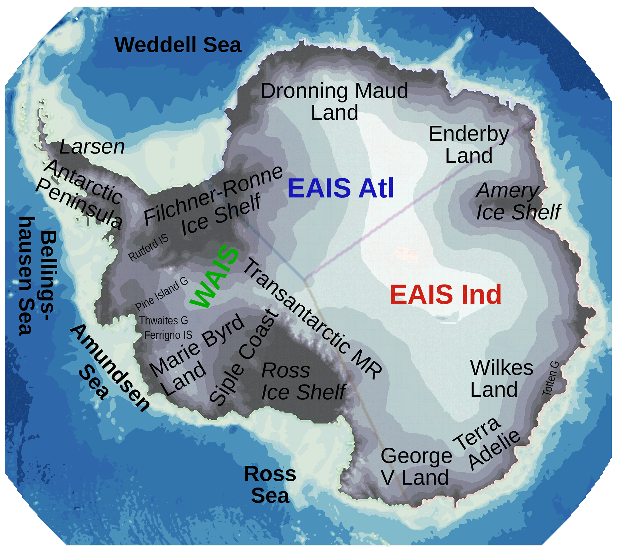
Figure 1Map of Antarctica. The seafloor depth is shown using a blue color scale, and the elevation of Antarctica above sea level is depicted using a dark-gray (low elevation) to white (high elevation) color bar. Ocean labels are displayed using bold font, and ice shelves are displayed using italic font. Labels with smaller font sizes show individual glaciers (G) and ice streams (IS). “MR” stands for “mountain range”. Colored labels define three regions: WAIS refers to the West Antarctic Ice Sheet (green), EAIS Atl refers to the East Antarctic Ice Sheet – Atlantic Sector (blue), and EAIS Ind refers to the East Antarctic Ice Sheet – Indian Ocean Sector (red). These regions are bound by the coastal areas and by their shared boundaries in the interior. Figs. 4 and 5 also show the boundaries of these regions. The bedrock topography and surface orography depicted here are taken from Fretwell et al. (2013).
1.3 Mass balance of Antarctica
Processes governing the balance between mass gain and mass loss determine if Antarctica contributes to a rising sea level. Antarctica's surface mass balance controls mass gain, whereas mass loss predominantly occurs due to ocean-driven basal melting of ice shelves and iceberg calving in concert with dynamical grounding line migration (Wingham et al., 2018). For individual ice shelves, the fraction between basal melting and iceberg calving ranges from 10 % to 90 % in the period from 1995 to 2009 (Depoorter et al., 2013). Estimates of the total mass loss agree within the uncertainties, even if they range from 2200 to 2800 Gt yr−1 (Depoorter et al., 2013; Liu et al., 2015; Rignot et al., 2013). However, they differ with respect to the relative contribution from basal melting and calving. Past studies have suggested that the overall mass loss is either driven by an almost equal share between calving (1321±144 Gt yr−1) and basal melting (1454±174 Gt yr−1) (Depoorter et al., 2013) or that the basal melting (1516±106 Gt yr−1) contribution is twice as high as the calving (755±24 Gt yr−1) contribution (Liu et al., 2015). The surface mass balance is the difference between mass gain by precipitation – here predominantly snowfall – and surface meltwater that runs off because it is not refrozen nor retained in the snowpack. Surface melt ponds (Kingslake et al., 2017) and runoff exist on Antarctic ice shelves (Bell et al., 2017), but their contribution to the total mass balance is considered to be negligible (Van Wessem et al., 2014), except for on the (northern) Antarctic Peninsula (Adusumilli et al., 2018).
The focus of this paper is to identify common features of an ensemble of ice sheet simulations forced by a multi-model forcing data set. After the discussion on the temporal and spatial evolution of the climatic boundary conditions from nine CMIP5 models, we diagnose the temperature scaling of the precipitation of these climate models. Afterwards, we investigate how the deduced scaling impacts the simulated ice sheet thickness in contrast to spatially homogeneous scaling (e.g., inferred from ice core data). Before we discuss our results and conclude, we estimate differences in Antarctica's sea level contribution for the variety of forcing and precipitation boundary conditions applied. Specific aspects of the work are compiled in the Appendix.
The full temporally and spatially varying forcings are obtained from a compilation of CMIP5 models representing a suite of climate scenarios. These climate forcings drive the Parallel Ice Sheet Model (PISM) in order to estimate Antarctica's future sea level contribution. Here, we test our hypothesis that the ansatz (implementation in a mathematical framework) of the precipitation determines whether the global sea level rises or falls. We consider two precipitation boundary conditions: (1) we utilize both the ocean and air temperature anomalies and the precipitation anomalies from CMIP5 models on top of the reference background distributions (see Table 2) that were used to drive the ice sheet model during spin-up; and (2) we take only the ocean and air temperature anomalies from CMIP5 models and compute the precipitation anomalies scaled by the air temperature anomalies. The second set of anomalies is also added to the reference fields (see Table 2). The second approach is commonly used, in particular, in paleo-applications (e.g., Applegate et al., 2012; Bakker et al., 2017; de Boer et al., 2013), while some sensitivity studies keep the surface mass balance constant (Feldmann and Levermann, 2015; Hughes et al., 2017). According to these pure thermodynamical considerations, negative temperature scaling is unexpected (Frieler et al., 2012); however, in reality, atmospheric dynamics may dominate in certain regions, calling the usage of constant scaling across Antarctica into question.
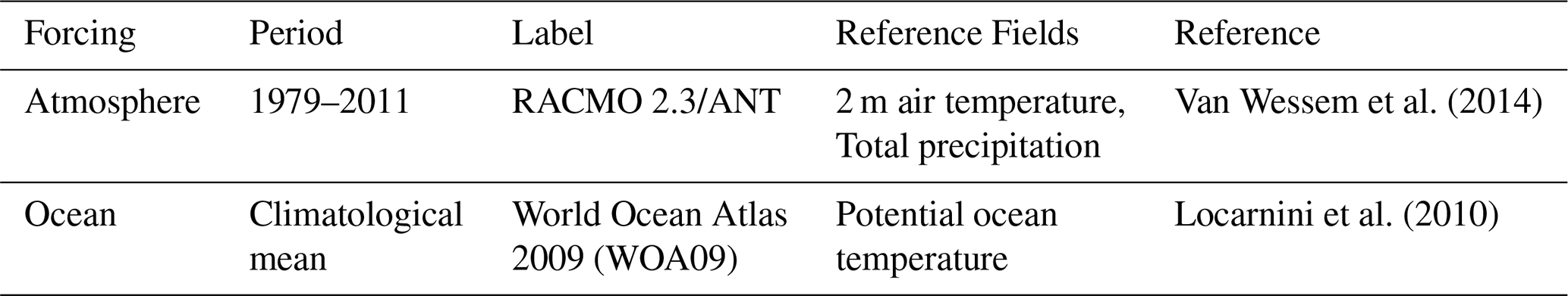
Van Wessem et al. (2014)Locarnini et al. (2010)Table 2Forcing used for ice sheet model spin-up and as reference fields for the anomaly forcing.
2.1 CMIP5 forcing data set to drive ice sheet simulations
Nine CMIP5 models deliver the following climate scenarios (see Table 1, Taylor et al., 2012): a control run under preindustrial conditions (piControl), the historical period (1850–2004), and RCP2.6, RCP4.5, and RCP8.5 (2005–2100) (Vuuren et al., 2011). These models stem from different model families (Knutti et al., 2013) and cover the range of current atmospheric (Agosta et al., 2015) and oceanographic (Sallée et al., 2013a) model uncertainties, although model deficiencies such as insufficient resolution can exist across all models. The transient forcing from 1850 to 2100 comprises the historical and scenario periods. Beyond 2100, the last 30 years (2071–2100) are repeated until the model year 5000. This procedure produces a chain of 30-year-long climate forcing periods that inherits the climate variability of this period – an alternative approach that involves repeating the last year (2100) would not contain any decadal variability.
The length of the control climate simulation (piControl) depends on the model and varies between 1 and 10 centuries (Table 1). From this control simulation, we extract the first or the last 50 years of the available forcing. As these two periods are subject to variation in the long-term variability as well as a potential long-term drift (identified by comparing both periods) during the control run, these two 50-year periods are generally slightly different. Therefore, anomaly forcing differs if it is computed relative to the first or last 50 years of control run. Hence, this procedure doubles the data set size of anomaly forcing. In the following, the first 50 years act as our reference.
The repetition of the last 30 years of climate forcing beyond the year 2100 is a simplification, which is not entirely consistent with the climate scenarios applied. An ongoing growing atmospheric greenhouse concentration would be expected to trigger changes in the climate system. While the atmospheric radiation reacts immediately, the redistribution of the accompanied heating within the global ocean is much slower (Hansen et al., 2011). This delay is critical because most of the additional heat ends up in the global ocean (Church et al., 2011, 2013b). Consequently, further warming is inevitable after the cessation of greenhouse gas emissions (Hansen et al., 2005). Note that our simulations do not reflect this ongoing warming. Furthermore, over longer timescales, some feedbacks are not captured by our simulations. For instance, a disintegrating Greenland Ice Sheet will increase the global sea level. As a consequence of Greenland's reduced gravitational pull (Whitehouse, 2018), the sea level rise is particularly pronounced around Antarctica (Mitrovica et al., 2001) due to the “remote” effect of gravitation. This rising sea level could potentially cause the grounding lines to migrate inshore, which would ultimately destabilize ice shelves and cause the Antarctic Ice Sheet to be more vulnerable. On the other hand, locally, the gravitational effect may buttress Antarctica if Antarctica's ice loss is slow enough (Gomez et al., 2010) and Greenland stabilizes. However, the ocean's ongoing thermal expansion is currently the dominant driver behind the rising sea level (Rietbroek et al., 2016). This rise will likely destabilize Antarctica. Therefore, as only 21st century climate conditions are used to force the ensemble after 2100, our ensemble of ice sheet simulations beyond this year should not be considered a projection.
Atmospheric and oceanic forcing is applied as annual mean forcing on top of the forcing used to spin-up the ice sheet model (Table 2). As CMIP5 models do not resolve ice shelves, ocean temperatures are extrapolated horizontally into the ice shelves to mimic isopycnic flow: the “fillmiss2” operator of the Climate Data Operators (, last access: 14 December 2020) tool kit acts on the original CMIP5 ocean grid. To allow for surface melting under a warming climate, the surface mass balance (SMB) is calculated following the positive-degree-day (PDD) approach (Braithwaite, 1995; Hock, 2005; Ohmura, 2001) as implemented in the PISM model (The PISM Authors, 2015a, b). Section 2.3 describes the PDD setup.
2.2 Parallel ice sheet model
The PISM ice sheet model – based on version 0.7 – runs on a 16 km equidistant polar stereographic grid and utilizes a hybrid system combining the shallow ice approximation (SIA) and shallow shelf approximation (SSA). The model employs a generalized version of the viscoelastic Lingle–Clark bedrock deformation model (Bueler et al., 2007; Lingle and Clark, 1985). In our simulations, only the viscous part was used due to known implementation flaws in the elastic part in our and later PISM versions. The basal resistance is described as plastic till by a Mohr–Coulomb formula to perform the yield stress computation (Bueler and Brown, 2009; Schoof, 2006). The basal melting of ice shelves is proportional to the squared thermal ocean temperature forcing (), which is the difference between the pressure-dependent melting temperature of the ice and the actual ocean temperature above melting. Here, the parameterization considers the full depth-dependence of the ocean temperature field, as described in Sutter et al. (2019). Basal ice shelf melting only occurs in fully floating grid points, and the grounding line position is determined on a sub-grid space (Feldmann et al., 2014) to interpolate basal friction.
The calving occurs at the ice shelf margin, and the three following sub-schemes determine it: (1) at the ocean–ice-shelf margin, ice shelf grid points with a thickness of less than 150 m calve; (2) ice shelves calve that extend across the continental shelf edge and progress into the deep ocean (defined by the 1500 m depth contour); (3) the Eigen-calving parameterization exploits the divergence of the strain or velocity field (Levermann et al., 2012), with the proportionality constant of 1×10¹⁸ or 1×10¹⁷ m s, respectively. Two independent spin-up runs delivering our initial conditions (PISM1Eq and PISM2Eq) utilize these constants. Ocean temperatures from the World Ocean Atlas 2009 (Locarnini et al., 2010) and the multiyear mean surface mass balance (SMB) from the RACMO 2.3/ANT model (Van Wessem et al., 2014) drive PISM during spin-up (Table 2). A similar model setup took part in the initMIP-Antarctica exercise under the name AWI_PISM1Eq with an adjusted Eigen-calving proportionality constant of 2×10¹⁸ and no bed deformation (Seroussi et al., 2019a).
2.3 Surface mass balance
The surface mass balance (SMB) is computed via the PDD method, where the hydrological year starts on day 91. The PDD factor values for snow and ice are 0.3296 and 0.8792 cm(IE) K−1 d−1, respectively (IE represents ice equivalent). The temporally evolving annual 2 m air temperature standard deviation is derived from daily CMIP5 model values for each CMIP5 model at each ice sheet model grid-cell.
The reference data set (Table 2) drives three special ice sheet control runs: “control 1”, “control 2”, and “control 3” (Table 3). These are performed to check whether a disturbance occurs when we replace the SMB used during the spin-up. The “control 1” simulation is a continuation of the spin-up, where the SMB (Fig. E16a) equals the precipitation from the reference data set (Table 2). The utilization of the PDD approach provides the SMB in “control 2”. In the “control 3” simulation, the SMB is computed via PDD and considers a potential height difference between the reference data set and the evolving ice sheet surface (Fig. E16b). For the height difference, we consider a lapse rate of −7 K km−1. As the height difference is zero at the beginning of this test, it initially does not influence the SMB. However, a lowering ice sheet surface in progressing simulations increases the air temperature used to compute the SMB via PDD. All of the SMB distributions (“control 1” to “control 3”) are numerically identical across Antarctica (Fig. E16c), because Antarctica is too cold to experience melting via PDD (Fig. 2a). (A detailed analysis of the climate follows in Sect. 3.1.) Therefore, the altered computation does not trigger any disturbance, although the SMB computed via PDD does allow for melting.

Figure 2CMIP5 data set mean anomalies (d–l) relative to the atmospheric (a, b) and oceanographic (c) reference forcing. The corresponding maximum and minimum fields are depicted in Figs. E1 and E2, respectively. Panels (a–c) represent the reference fields to spin the ice sheet model up (Table 2). The 2 m air temperature (a) and the total precipitation (b) are mean fields from the regional RACMO model, and the ocean temperatures (c) come from the World Ocean Atlas 2009; see Table 2 for more details. The color bar for each reference field is given above the respective plot. Below each reference field, the related anomalies, including their color bar, are compiled for the period from 2071 to 2100. Here, the second, third, and fourth rows show the anomalies for RCP8.5, RCP4.5, and RCP2.6, respectively. In these atmospheric anomaly plots, the dark-gray line follows the current coastline. All potential ocean temperatures (c, f, i, l) are a vertical mean of the depth interval from 150 to 500 m. The white contour lines in the anomaly plots (e, h, k) highlight the 30 cm yr−1 precipitation threshold. All of these anomalies are the CMIP5 model means of the models listed in Table 1; CCSM4 is not part of RCP2.6. Antarctica's contours are deduced from Fretwell et al. (2013).
Table 3Members of the ice sheet model ensemble. The second column “D/A” indicates if forcing has been applied directly “D” or as an anomaly “A”. The third column, “SMB”, represents the surface mass balance, where “PDD” is the positive-degree-day approach, and “LR” indicates the use of an air temperature correction due to a local ice surface height difference utilizing a constant lapse rate. If the entry is “precipitation”, the precipitation of the forcing data set equals the surface mass balance. The “control 1” to “control 3” simulations are driven by the reference data sets (Table 2). Other ice sheet simulations are forced by anomalies on top of the reference data sets. These anomalies are computed relative to the first and last 50 years of the available piControl simulations. We utilize the following CMIP5 scenarios: “piCtrl” – “piControl”; “hist” – “historical”; “RCP2.6”; “RCP4.5”; and “RCP8.5” (Table 1). The CMIP5 scenario “hist” represents the historical period from 1850 to 2004, and the three projections “RCP2.6”, “RCP4.5”, and “RCP8.5” cover the period from 2005 to 2100. Beyond the year 2100, the forcing of the last 30 years (2071–2100) is recurrently applied until the model year 5000. The data set comprises 26 anomaly forcing scenarios. Each scenario starts from the PISM1Eq (Fig. E10) and PISM2Eq (Fig. E11) initial conditions and is driven by two precipitation conditions (see Sect. 2.3 and 2.4 for details). Hence, the ensemble of anomaly ice sheet simulations has 208 members in addition to “control” runs.

2.4 Precipitation scaling
Inspired by the Clausius–Clapeyron process, it is often assumed that precipitation also increases with a warming atmosphere. Along with the contemporary climate fields as a reference, the air temperature scaling of precipitation is
where ΔT is the air temperature anomaly, ΔP is the precipitation anomaly, and is the precipitation reference field. The scaled precipitation is
As reported above (Sect. 1.2), in the modeling context, it is often assumed that the scaling is constant: .
Depending on the CMIP5 forcing scenario applied, the ensemble mean climate signal is weaker for those scenarios following an aggressive mitigation path and, hence, releasing less carbon dioxide (e.g., RCP2.6). Around Antarctica, the ensemble analyzed here follows the same pattern (Figs. 2 and 3). As greenhouse gas concentrations have most closely followed the high-emission RCP8.5 scenario path over the past decade, we will focus on RCP8.5 if not otherwise stated.
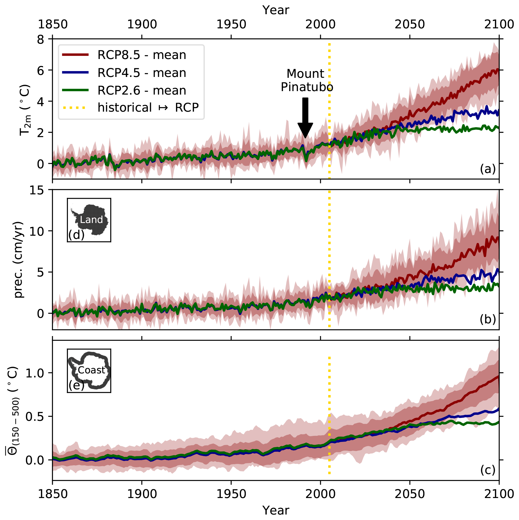
Figure 3Spatial mean of the (a) 2 m air temperature and (b) total precipitation anomalies on Antarctica (d). Spatial mean of the (c) potential ocean temperature that is averaged over the depth interval from 150 to 500 m in the coastal zone surrounding Antarctica. In subfigure (e), the dark region defines the coastal zone. The CMIP5 data set mean values are shown for the scenarios according to the legend in panel (a). The dark-red band highlights the 1σ standard deviation (66 %), and the light-red band shows the full range covered by all CMIP5 models for RCP8.5 only. The vertical golden line marks the transition from the historical forcing to the RCP. The distinct air temperature jump during the historical period in 1991 marks the Mount Pinatubo volcanic eruption. The contours of the Antarctic continent (d) follow the outer edges defined by the data set of Fretwell et al. (2013), whereas the coastal strip (e) is an extension into the sea with smoothed northern edges (typical width of about 500 km).
3.1 CMIP5 forcing data set
From 1850 until the end of the 21st century, the CMIP5 data set spatial mean 2 m air temperature in Antarctica (see the map in Fig. 3d) rises steadily by 6 K with a spread of 1 K (1 standard deviation; Fig. 3a), and the mean precipitation also accumulates by 9±3 cm yr−1 (water equivalent; Fig. 3b). The average potential ocean temperature in the depth range from 150 to 500 m along Antarctica's coast (see the map in Fig. 3e) warms by nearly 1±0.18 ∘C during the same period (Fig. 3c). In particular, these warming trends have become stronger in the atmosphere and ocean since the beginning of the 21st century.
3.1.1 Spatial patterns in the atmosphere
These changes are not homogeneous across the Antarctic continent (Fig. 2d–l). The atmosphere warms most strongly along the Antarctic Peninsula (which is in agreement with the current observed trends; Mulvaney et al., 2012; Thomas et al., 2009), the high plateau of the East Antarctic Ice Sheet (EAIS), and, to a lesser degree, around the Filchner–Ronne Ice Shelf region (Fig. 2d, g, j). The warming is lowest in the coastal areas of East and West Antarctica that extend (clockwise) from the Greenwich Meridian via Wilkes Land and the Ross Ice Shelf to Marie Byrd Land, respectively. The Amery Ice Shelf interrupts the coastal band of low 2 m air temperature rise. In general, warming trends are less pronounced over the adjacent ocean and ice sheet interior.
The precipitation increases marginally across the high plateau of the EAIS and east of the Ross Ice Shelf as part of the WAIS (Fig. 2e, h, k). In contrast, the coastal areas, where air masses with a lot of precipitable water make landfall, receive more precipitation. As these air masses on their way into the interior are uplifted by the steep topography, the precipitation along the coasts is topographically controlled. Areas of heavy precipitation under the reference climate (Fig. 2b) also receive the highest increments. The precipitation increases most strongly along the western Antarctic Peninsula, where the lifting of eastward-flowing air masses by mountain ranges leads to topographic precipitation, which is firmly enhanced; this resembles the observed positive precipitation trend in the Antarctic Peninsula since 1900 (Wang et al., 2017).
3.1.2 Spatial patterns in the ocean
Under the control climate, the coldest potential ocean temperatures in the depth range from 150 to 500 m exist offshore of the coasts of Antarctica (Fig. 2c). We detect the lowest ocean temperatures in front of the Filchner–Ronne, Amery, and Ross ice shelves. Furthermore, the Amundsen Sea in front of Pine Island and Thwaites glaciers is cold.
The subsurface ocean temperature warms vigorously along sections of the Antarctic Circumpolar Current (ACC) and in the western Weddell Sea at the center of the ocean gyre. For instance, the warm spot in the western Weddell Sea emerges in all CMIP5 models (Fig. 2f, i, l). In the coastal strip surrounding Antarctica, the warming is of medium strength and is heterogeneous. In the region, the most robust warming appears in the Amundsen Sea and along the coast of the EAIS (between Wilkes Land and Terre Adélie) opposite Australia. The least warming occurs in front of both the western Ross and Filchner–Ronne ice shelves and the neighboring Antarctic Peninsula, where the ocean temperatures are lowest in the control climate (Fig. 2c).
3.1.3 CMIP5 data set as ice sheet model forcing
The spatial structure of the anomalies discussed above is generally independent of the forcing scenario applied; however, the scenarios determine the strength of the anomalies. Regardless of the scenario applied, the discussion of the atmospheric climate anomalies already indicates that both precipitation and air temperature do not necessarily correlate. Instead, regional differences are evident, and a simple scaling of the precipitation with temperature appears to be inadequate.
In front of the Filchner–Ronne, Amery, and Ross ice shelves as well as in the Amundsen Sea, the climatological ocean temperature distribution might be too cold because it does not replicate the confined flow of warm water masses through glacier-scoured troughs towards ice shelves (see Appendix A). To overcome this limitation, we apply a spatially restricted melting correction. The correction increases the melting by 50 % for the Ronne Ice Shelf region, and it quadruples melting for coastal parts of the West Antarctic Ice Sheet between the Antarctic Peninsula and the Getz Ice Shelf (east of the Ross Ice Shelf).
3.2 Precipitation scaling across Antarctica
Ice sheet simulations bridging several millennia often rely on climate anomalies deduced from sources such as ice cores. Based on the isotopic signatures in ice cores, temperature anomalies are deduced. Inferred accumulation anomalies from these cores are converted into precipitation anomalies. The scaling deduced from ice cores varies between 5 % K−1 and 7 % K−1 in Antarctica, with a 2σ uncertainty of about 1 % K−1–3 % K−1 (Fig. 4, Table 4).
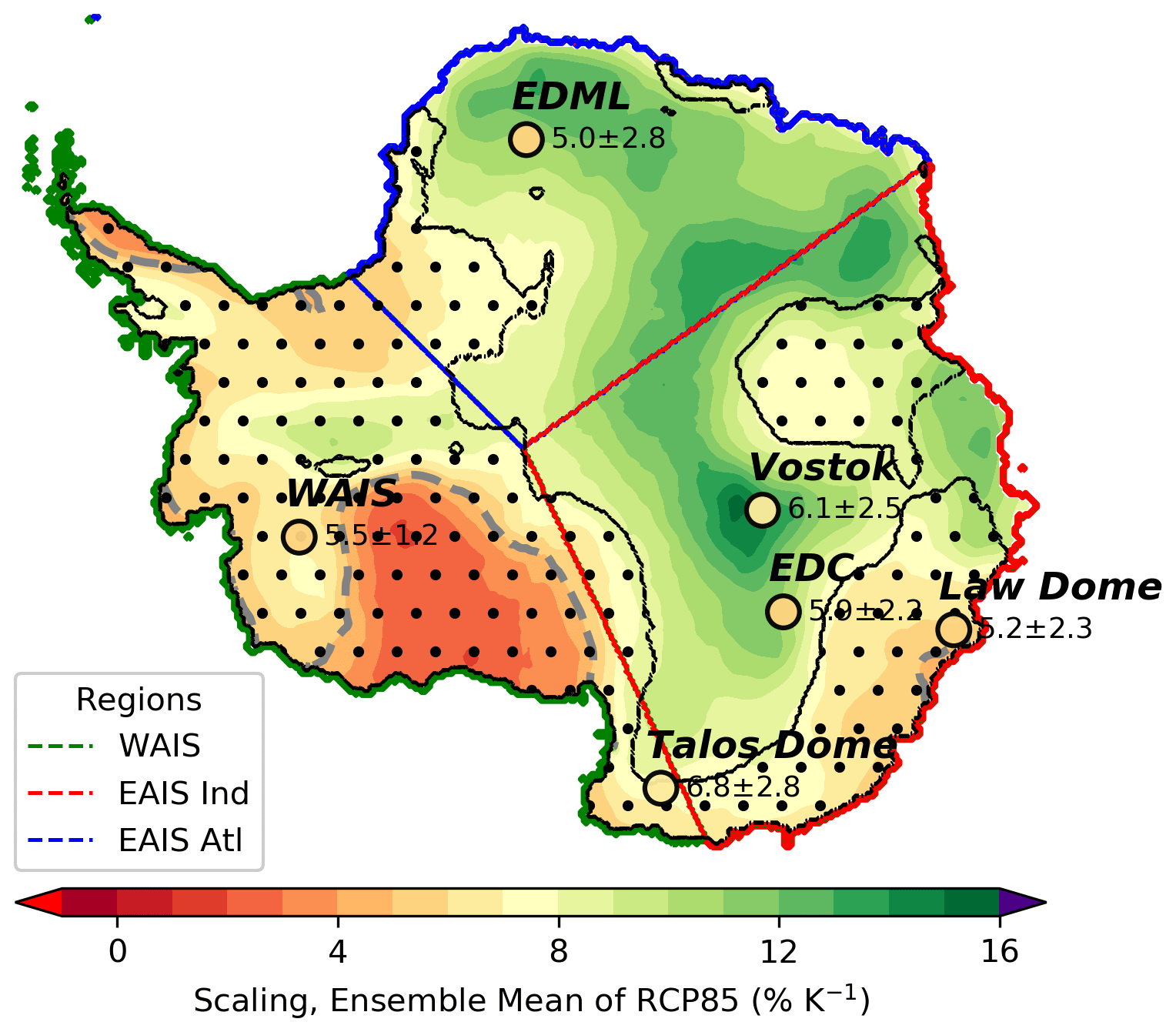
Figure 4CMIP5 data set mean of the temperature-scaled precipitation for the period from 2051 to 2100. This scaling under the RCP8.5 scenario comes from nine CMIP5 models (Table 1), which are driven by anomalies relative to the first 50 years of piControl. In the dotted regions enclosed by black contours, the combined simulated scaling and the standard deviation contain the value of 5 % K−1. Gray dashed lines follow this 5 % K−1 contour. The scaling values deduced from ice cores are shown at their location (Frieler et al., 2015) using the same color bar as the spatial distribution within the circle. The neighboring printed values are the mean and the 2σ uncertainty. Three defined regions (Table 5) named “WAIS”, “EAIS Atl”, and “EAIS Ind” are outlined using green, blue, and red boundaries (lower left legend), respectively. For further details, the reader is referred to Sect. 3.2. Figure E3 provides the corresponding distributions for each CMIP5 model. Antarctica's contour is deduced from Fretwell et al. (2013).
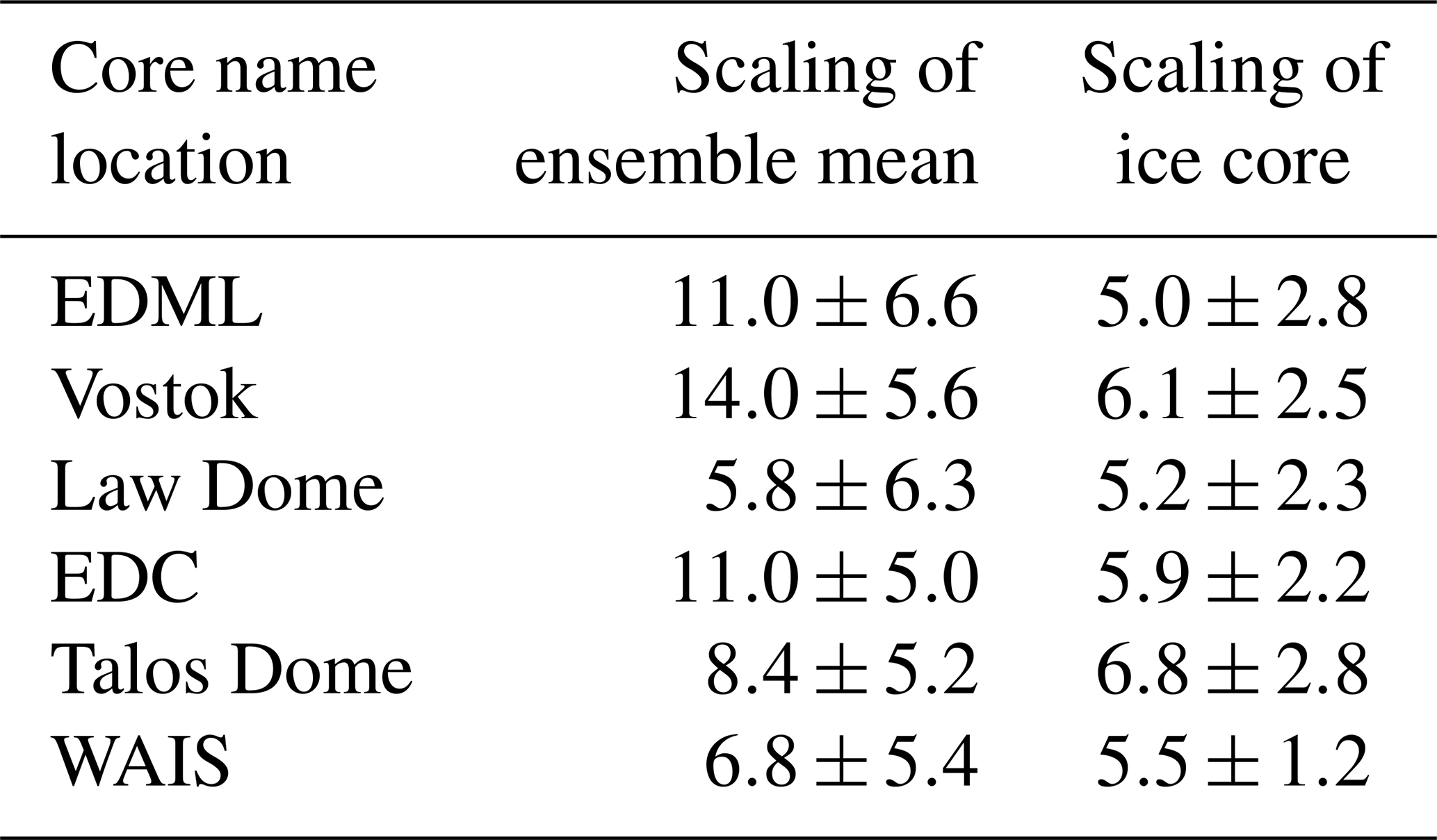
Table 4Air temperature scaling of the precipitation for six ice core locations in Antarctica. The second column lists the ensemble mean scaling (RCP8.5, first 50 years, both the PISM1Eq and PISM2Eq initial states) and standard deviation (2σ) across all ensemble members. The third column provides scaling factors deduced from ice cores (Frieler et al., 2015), including the provided error margins (2σ). The reader is referred to Fig. 4 for the ice core locations.
3.2.1 Spatial pattern of precipitation scaling in the CMIP5 data set
The corresponding average CMIP5 scaling is generally larger than observational estimates at these ice core locations (Table 4). At the Vostok ice core location, the difference is most conspicuous, and the simulated scaling is more than twice as large as the observed scaling. For the EDML and EDC locations (Fig. 4), there are also substantial differences of around a factor of 2. In contrast, the scaling of the Law Dome, Talos Dome, and WAIS ice cores are indistinguishable from the corresponding CMIP5 average within the uncertainties. Here, we have computed the scaling by averaging the precipitation of the piControl run (first 50 years) to obtain the reference data (baseline) and the last 50 years of the RCP8.5 scenario from 2051 to 2100 to get the anomalies.
To test the result's robustness, we exchange the baseline: the beginning of the historical period is used instead of the first 50 years of piControl. Both the first 50 years of piControl and the historical forcing (1850–1899) start from the same state but are subject to diverging forcing, e.g., in atmospheric greenhouse gases and volcanic events (such as Krakatau in 1883; Henderson and Henderson, 2009). Despite replacing the baseline, the values change only slightly. As the results are very similar when exchanging the baseline, we restrict the analysis to anomalies relative to the first 50 years of the piControl climate and consider the results robust.
The spatial distribution of the scaling derived from our CMIP5 data set is heterogeneous and varies more strongly than the ice core data suggest. Values between 4 % K−1 and 6 % K−1 occur at the Filchner–Ronne Ice Shelf and in the coastal Terre Adélie region (see the map in Fig. 1 for place names). On the WAIS, these values are also present in the coastal strip from the Antarctic Peninsula to the Ross Ice Shelf and along the Transantarctic mountain range's eastern flank (Fig. 4).
The highest scaling factor emerges on the EAIS, where a c-shaped part of the high plateau has factors exceeding 12 % K−1. This area reaches out to Dronning Maud Land, which also has very high scaling factors. The West Antarctic Ice Sheet has scaling factors that are generally lower than 8 % K−1, and values of up to 10 % K−1 are only detected in the elevated interior. Over the Ross Ice Shelf and the eastward adjacent Siple Coast, scaling factors are the lowest (Fig. 4). As we detect heightened scaling factors in some places at high elevation, we aimed to determine whether we could find a relationship between elevation and scaling. However, we could not identify a robust relationship (not shown) for the entire Antarctic continent nor for defined subregions (see below).
3.2.2 Precipitation scaling across regions in Antarctica
Our analysis now focuses on the scaling factors of all grounded ice, which, if lost, contributes to a rising potential sea level. Additionally, we analyze the scaling factors for the entire continent (label “glaciered”), and four glaciated regions labeled “EAIS Atl”, “EAIS Ind”, “WAIS”, and “Siple Coast” (Fig. 5 and Table 5). We detect a slight trend towards higher values if we restrict the analysis to ground ice (87.5 % of the glaciated area; see Table 5). However, the scenario selection is decisive, whereas the choice between “glaciered” and “grounded” is unessential for the CMIP5 mean. In general, individual CMIP5 models show the same result. The sensitivity of many CMIP5 models to the range of the scenario applied is within their variability (e.g., CSIRO-Mk3-6-0, CNRM-CM5, MIROC-ESM, and MRI-CGCM3) or may hint at an enlarged scaling for weaker scenarios (e.g., MPI-ESM-LR). Frieler et al. (2015) found a low dependence of the scaling factors to four RCP scenarios for the whole Antarctic continent. Anomalies are not as distinctly pronounced in RCP2.6 as in the other scenarios due to the weaker forcing scenario. Note that RCP2.6 is missing for CCSM4 (hence, we have hatched the corresponding bar).
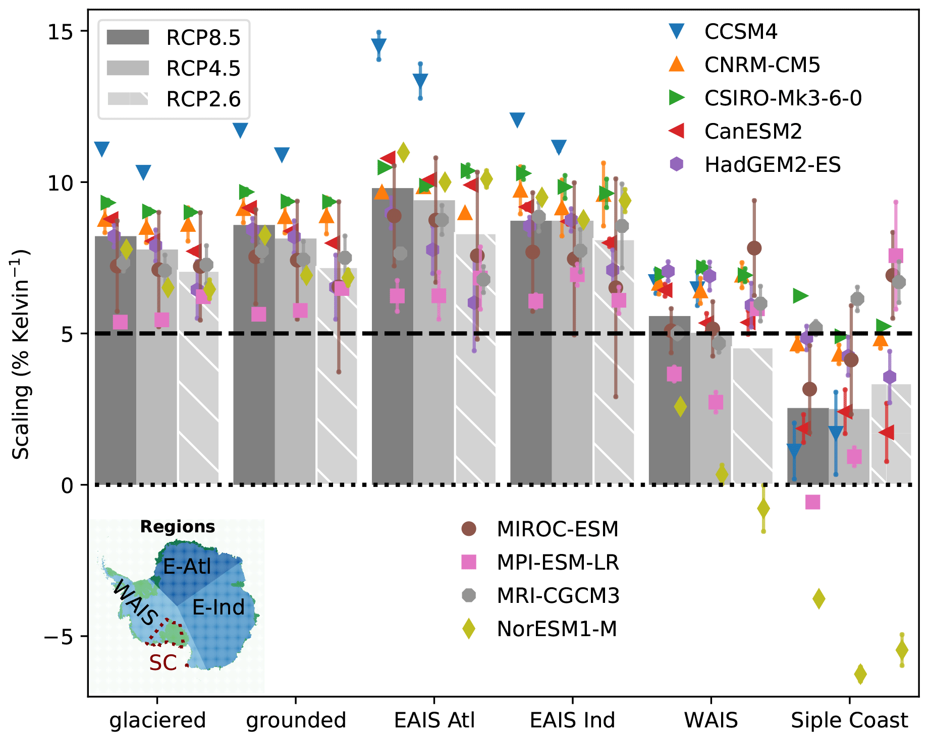
Figure 5Air temperature–precipitation scaling deduced for the nine CMIP5 models (Table 1) and three future scenarios (legend) in six defined regions in Antarctica (see the map in the lower-left corner and Table 5). The coastlines and the grounding line positions are deduced from Fretwell et al. (2013). The gray bars represent the CMIP5 data set average, and the individual symbols stand for CMIP5 models. Here, the results apply for both reference periods, where the anomalies are computed relative to the first or last 50 years of piControl. Each symbol is the model average of both reference periods, and the attached line indicates the scatter range between the first and last 50-year reference periods. Note that the RCP2.6 scenario does not include the CCSM4 model; hence, the corresponding bar is hatched.
Table 5Defined areas as part of our diagnostic. The fraction is computed relative to “glaciered”. Figures 1, 4, and 5 depict these areas.
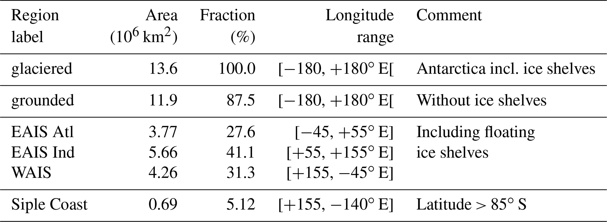
The boundaries of the three regions “EAIS Atl”, “EAIS Ind”, and “WAIS” resemble different oceanographic zones (Whitworth III et al., 2013; Orsi et al., 1999; Foldvik and Gammelsrød, 1988) when Antarctica's large-scale drainage basins are taken into account (Zwally et al., 2015). This chosen division of Antarctica does not produce surface areas of equal size. As already indicated by the spatial distribution (Fig. 4), the order of the scaling factors from high to low would be “EAIS Atl”, “EAIS Ind”, and “WAIS”. The difference between both “EAIS” regions is minor, with a tendency towards higher values in “EAIS Atl” in the CMIP5 mean and some individual CMIP5 models. Some models do not show a clear trend between the scenario strength and scaling factor. For example, the scaling decreases in “EAIS Atl” from RCP4.5 over RCP8.5 to RCP2.6 for MRI-CGCM3, whereas in “EAIS Ind” the order is from RCP8.5 over RCP2.6 to RCP4.5 (Fig. 5). This again indicates that regional differences matter.
The “WAIS” region has significantly lower scaling factors than both “EAIS” regions. This difference exists for the CMIP5 model average regardless of the scenarios applied and for almost all individual CMIP5 models (Fig. E3). Exceptions are MIROC-ESM and MPI-ESM-LR under the RCP2.6 scenario and HadGEM2-ES under all scenarios.
3.3 Sea level impact of precipitation scaling by air temperature
To understand how the precipitation boundary condition impacts Antarctica's contribution to the global sea level, we inspect the precipitation falling on Antarctica (Fig. 6). Therefore, the precipitation is integrated over time since 1850 and across the dark-blue masked region representing grounded ice (map in Fig. 6). This analysis is restricted to all CMIP5 models driven by RCP8.5 and anomalies computed relative to the first 50 years of the control run. As accumulated precipitation integrated over Antarctica lowers the global sea level under the assumption that ice loss (basal melting or calving) does not occur, the temporally accumulated potential sea level impact curves have a negative slope (Fig. 6a, b). Hereafter, this quantity is labeled “integrated precipitation.”
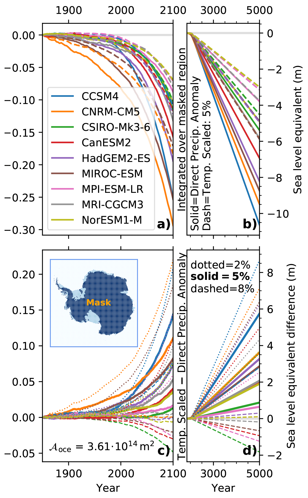
Figure 6Panels (a) and (b) show the integrated potential sea level equivalent of the precipitation falling on grounded ice in Antarctica (see the dark-blue mask in the lower left, where the light-blue parts highlight ice shelves); the grounded and floating ice areas are derived from Fretwell et al. (2013) for the anomaly forcing (solid lines) and temperature-scaled precipitation (dashed lines) considering a scaling of 5 % K−1. The difference in the potential sea level impact between the anomalies and the temperature-scaled precipitation is depicted in panels (c) and (d). Here, the solid lines consider scaling of 5 % K−1, and the dotted and dashed lines consider a scaling of 2 % K−1 and 8 % K−1, respectively. Panels (a) and (c) are restricted to the period from 1850 to 2100, whereas panels (b) and (d) cover the full period from 1850 to 5000. Every single colored line (see the legend in a) represents one CMIP5 model (Table 1). The corresponding curves for the RCP4.5 scenario as well as for a different mask that covers the entire continent are available in Fig. E4.
In this paper, we distinguish between potential or diagnosed sea level and simulated sea level. The potential sea level is the transformation of an ice mass or freshwater volume into a global sea level by applying a global ocean area of 3.61×10¹⁴ m2 (Gill, 1982). In contrast, the simulated sea level is a diagnostic of the ice sheet model, which takes the released total mass above flotation and the global ocean area into account.
The integrated precipitation declines more forcefully from the beginning of the 21st century, which is driven by the concurrent increase in precipitation over Antarctica (Fig. 3b). The integrated precipitation shows a more pronounced temporal change than the mean precipitation (Fig. 3b), because the vast interior, characterized by light precipitation, dominates the integral. After the year 2100, the integrated precipitation declines linearly (Fig. 6b), as we adopt the forcing of the years 2071–2100 recurrently. By applying the actual precipitation anomalies (solid lines, Fig. 6a, b), the potential sea level drop is stronger than using a scaling of 5 % K−1 (dashed lines, Fig. 6b) because the models' internal scaling exceeds 5 % K−1 (Fig. 5). In the year 5000, the sea level drop ranges from 5 to 11 m when applying simulated precipitation anomalies and from just 3 to 6 m when using the 5 % K−1 scaling.
The difference in the integrated precipitation between 5 % K−1 scaled and directly applied precipitation anomalies is always positive (solid lines in Fig. 6c, d). This difference ranges approximately from 1 cm (CSIRO-Mk3-6-0) to 15 cm (CCSM4) in the year 2100 and from 60 cm (MPI-ESM-LR) to 550 cm (CCSM4) in the year 5000.
A lower scaling of 2 % K−1 causes a magnified difference (dotted lines in Fig. 6c, d). Ultimately, it corresponds to a reduced potential sea level contribution. This leads to differences ranging from 5 cm (MPI-ESM-LR) to 21 cm (CNRM-CM5) in 2100 and from 150 cm (MPI-ESM-LR) to 850 cm (CCSM4) in 5000.
A higher scaling of 8 % K−1 (dashed line in Fig. 6c, d) exceeds ice-core-based estimates (Table 4, Fig. 4), whereas it approximately corresponds to the CMIP5 data set average (RCP8.5 ≈ 8.2 % K−1 and RCP4.5 ≈ 7.8 % K−1; Fig. 5). Now, only the CCSM4 model exhibits a positive difference because its scaling reaches 11 % K−1 (Fig. 5). Four models are nearly balanced (CNRM-CM5, MRI-CGCM3, HadGEM2-ES, and NorESM1-M), whereas the remaining four feature negative differences (CSIRO-Mk3-6-0, CanESM2, MIROC-ESM, and MPI-ESM-LR). Hence, the difference range is subject to a change in sign, and the individual differences range from −5 cm (CSIRO-Mk3-6-0) to 7 cm (CCSM4) in 2100 and from −170 cm (CSIRO-Mk3-6-0) to 280 cm (CCSM4) in 5000.
3.4 Relation between precipitation boundary condition and ice sheet thickness
For the diagnostic of the relation between precipitation and ice sheet thickness, we inspect the ensemble mean (average across all ice sheet simulations) as well as the maximum and minimum thickness at each grid point across all ensemble members. Therefore, the field of joined extreme values could come from a diverse set of ice sheet ensemble members and, hence, does not necessarily lead to a dynamically consistent distribution.
Some ice sheet simulations (“control 3”, Table 3) are driven solely by the reference forcing fields (Fig. 2a–c), e.g., they neglect any anomaly. In these simulations, the detected trend of about 2 mm per decade (sea level equivalent) fades within the first 400 years and differs slightly between the two initial states (PISM1Eq and PISM2Eq). Even if we apply anomalies on top of the reference background fields, we can not entirely exclude a shock-like behavior of the simulations directly following the decades after the year 1850. As we compute the anomalies relative to the average over the respective first or the last 50 years of the control run for each climate model, these anomalies are not necessarily zero at the beginning of the year 1850. Hence, the ice sheet model may experience a small jump, which causes an initial artificial trend.
In the year 2100, the ice thickness for both precipitation boundary conditions (precipitation anomaly deduced from the applied climate models vs. scaled precipitation) increase over large parts of the Antarctic continent (Fig. 7b–e). The thickness for the simulations driven by scaled precipitation grows less over substantial parts of the interior than in the simulations forced by the precipitation anomalies (Fig. 7a), as the difference between scaled precipitation and applied precipitation anomaly is mostly negative. This pattern explains the diagnostic, where the sea level drop is weak for temperature-scaled precipitation with a scaling of 5 % K−1 (Fig. 6).
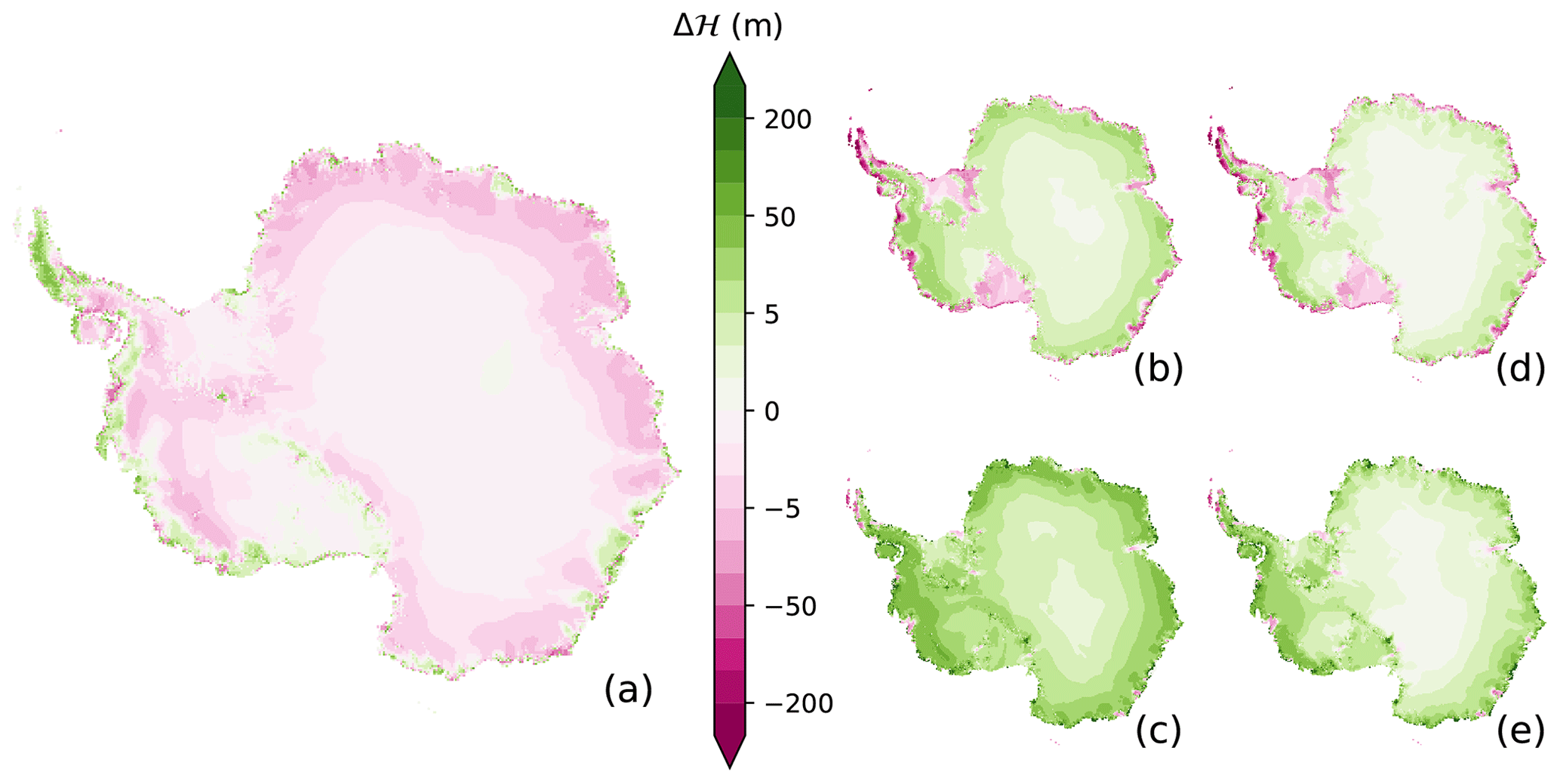
Figure 7Ice thickness changes under the RCP8.5 scenario in the year 2100 since the year 1850. The ensemble mean difference between the runs forced by the scaled precipitation and the precipitation anomalies (a). For each climate model scenario, the anomalies are computed relative to the 50 years of the related piControl scenario. The simulations driven with the precipitation anomaly (b, c) have the mean ice thickness (b), and the maximum ice thickness (c) changes. The temperature-scaled precipitation of 5 % K−1 gives the corresponding ensemble mean (d) and maximum (e). Please note that all subplots share the same color bar, and panel (a) equals panel (d) minus panel (b).
A ring of a pronounced negative thickness difference exists along the coast. This ring emerges for a significant part of the coastal East Antarctic Ice Sheet (EAIS) and West Antarctic Ice Sheet (WAIS). For the latter ice sheet, the negative area is shifted away from the coast towards the interior (Fig. 7a). A negative strip of the thickness difference appears on the southern side of the Transantarctic mountain range and for some grounded ice streams flowing into the Filchner–Ronne Ice Shelf.
Regions of positive differences coincide with thicker ice for simulations driven by scaled precipitation. These are located south of the Transantarctic mountain range at the northern edge of the Ross Ice Shelf, along the coastline of the WAIS, and in the coastal Terre Adélie region. In these regions, the scaling is generally lower or falls behind the constant scaling of 5 % K−1. However, this does not explain exclusively positive areas.
For both precipitation boundary conditions, the mean ice thickness of each of the respective sub-ensembles reveals a widespread weakening of the floating ice shelves, such as the Filchner–Ronne, Ross, and Amery ice shelves (Figure 7b, d). In the WAIS, both Pine Island Glacier and Ferrigno Ice Stream (an ice stream that flows into the Filchner Ice Shelf) thin drastically. Along the Antarctic Peninsula, general shrinking occurs along the coasts. Ice also thins along the coasts of the EAIS.
For some places, the ice thickness thins for both precipitation boundary conditions across all ensemble members, as the reduction in the maximal ice thickness highlights (Fig. 9c, e). This reduction marks those outlet glaciers and ice shelves that are extremely vulnerable. These are around the Rutford Ice Stream, Foundation Ice Stream, Ronne Ice Shelf, Amery Ice Shelf, three outlet glaciers (in “EAIS Ind” as part of Wilkes Land, Terre Adélie, and George V Land), the northwestern Ross Ice Shelf (Ross Island), and Pine Island and Thwaites glaciers in the Amundsen Sea (Fig. 9c, e).
3.5 Precipitation boundary condition and sea level
In the following, we consider the entire ensemble (Table 3). Ensemble members start from both the PISM1Eq and PISM2Eq initial states, they are driven by all climate scenarios (historical followed by RCP2.6, RPC4.5, or RCP8.5; Table 2), and the anomalies are computed relative to the first or last 50 years of the related control run (piControl). The simulated sea level curves are shifted so that the simulated sea level contribution is 0 m in the year 2000 (Fig. 8). As the spread of individual ensemble members may not follow a normal distribution, in addition to the mean, we also present the median sea level contribution. For the RCP8.5 scenario, we highlight the spread among models by depicting the standard deviation (1σ).
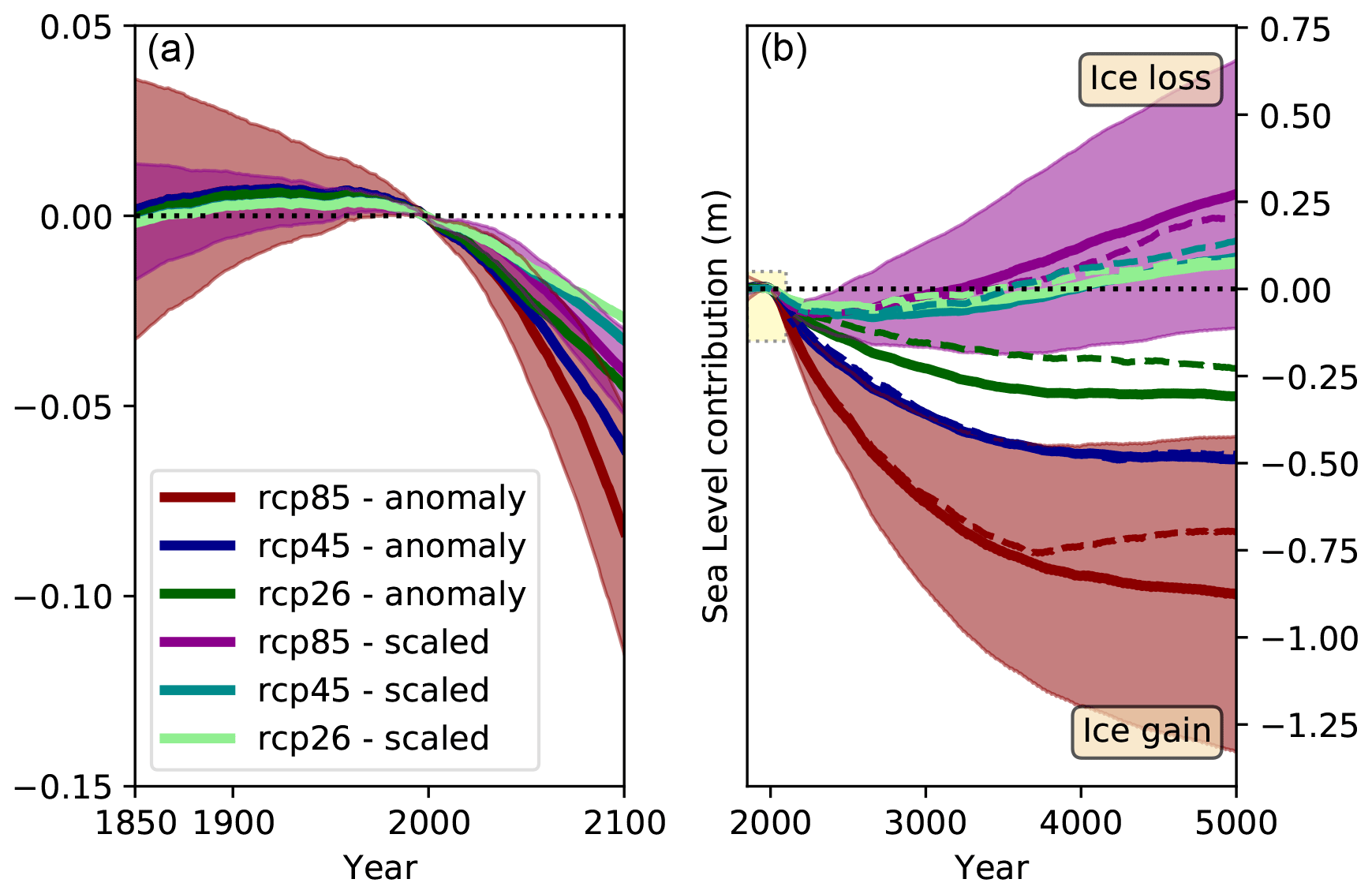
Figure 8Sea level contribution of Antarctica computed by the ensemble of ice sheet simulations (see Sect. 3.5 for details). The solid lines represent the ensemble averages for the applied precipitation anomalies and the air-temperature-scaled precipitation boundary conditions according to the legend (panel a), and the dashed lines are the corresponding medians. For the RCP8.5 scenario, the shading highlights the standard deviation (1σ) as a measure of the variability among the ice sheet ensemble members driven by various climate models (Table 1).
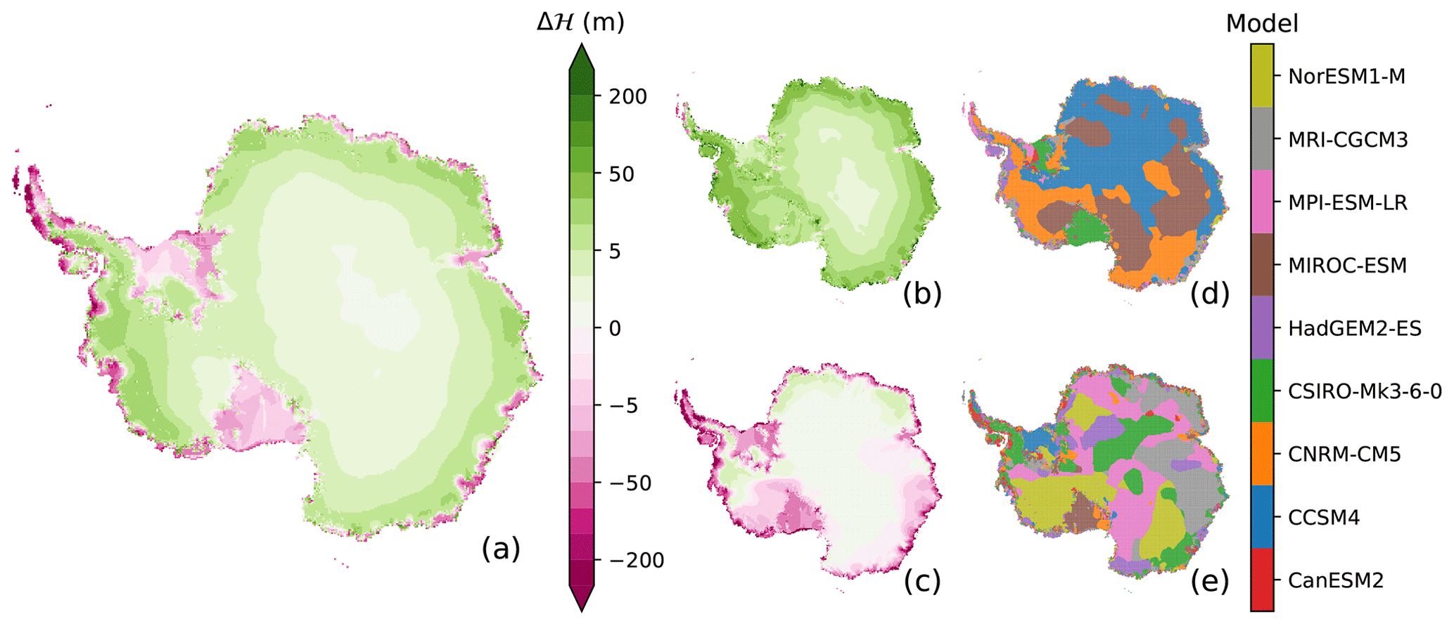
Figure 9Ice thickness changes since 1850 under the RCP8.5 scenario for the precipitation anomaly that was actually applied in the year 2100. Highlighted are the ensemble mean (a), ensemble maximum (b), and ensemble minimum (c). The climate models that were used to drive the ice sheet model simulation causing the maximum and minimum thickness are shown in panels (d) and (e), respectively, next to the ensemble maximum (b) and minimum (c).
For the period from 1850 to 2000, the simulated sea level contribution of Antarctica fluctuates slightly. Hence, the accumulation almost balances the ice loss at the margin, and the basal melting rates of grounded ice are steady (Fig. E9). Note that there is no drift involved, as we have subtracted the trend from the continued ice sheet simulations under the reference climate (Table 2). We also detect an amplified signal for the simulations driven by the precipitation anomalies compared with those forced by temperature-scaled precipitation anomalies, which corresponds to the abovementioned sea level impact of precipitation (Fig. 6).
After the year 2000, all of our ensemble members, regardless of the forcing scenario, gain mass, causing a falling simulated sea level (Fig. 8). The basal melting of grounded ice does not affect the sea level evolution, because this basal melting rate is nearly constant and negligible. Hence, the corresponding integrated sea level equivalent grows linearly for all scenarios from 1850 to 2100, and these curves only diverge after the year 2500 (Fig. E9). Moreover, the combined loss of iceberg calving and the basal melting of floating ice shelves does not vary considerably over the period considered. Consequently, the growth of simulated accumulation explains the net mass gains and, hence, the negative sea level contributions from Antarctica after the year 2000 (Fig. 8). Depending on the applied forcing and precipitation boundary condition, the global simulated sea level drop ranges from 2 to 11 cm until 2100 (Fig. 8). This result is in contrast to various publications, and we discuss it in the following.
If we continue our ensemble with the last 30 years of forcing until the year 5000, the simulated sea level contribution of the ensemble members driven by the temperature-scaled precipitation starts to stabilize and reaches a minimum around the year 2500 (Fig. 8). Afterward, they begin to lose more ice at the margins than they gain in the interior. As a consequence, these simulations produce on average a positive contribution to the global simulated sea level after the year 3200 (RCP8.5) and 3900 (RCP2.6), which compensates for the negative contributions since 1850. In the year 5000 at the end of our simulations, these simulations show a trend towards a continuously growing ice loss rate, because the curves still have an tendency that is directed upward. Hence a quasi-equilibrium is not established. In contrast, the simulations driven by the precipitation anomalies continue to show a falling simulated sea level. They always contribute negatively to the global simulated sea level until the year 5000. Their ensemble mean and median sea levels tend to converge towards a new equilibrium at the end of the simulations (Fig. 8).
In all CMIP5 models, the 2 m air temperature warms across the entire Antarctic continent without any exception (Figs. 2d, g, j, 3a), because even the minimum 2 m air temperature anomaly is positive everywhere (Fig. E2d, g, j). The warming enhances the hydrological cycle, which generally causes heavier precipitation (Fig. 3b), in particular along the coast of Antarctica (Fig. 2e, h, k). However, the changing precipitation does not increase at the same rate as increasing air temperature because it is not only thermodynamically influenced but also dynamically controlled. Given that the ensemble mean temperature scaling is different for the West and East Antarctic Ice Sheet (Fig. 5) and has a considerable spatial dependence, the dynamical component is not negligible. Instead, the region of reduced precipitation under rising air temperatures, which we have identified along the Siple Coast, highlights that the dynamics could compensate for or even overwhelm the impact of thermodynamics. The continent-wide scaling is inherently problematic, even if we were to adjust the scaling factor to reproduce the continent-wide average scaling. In this case, the integrated precipitation would be identical, but the spatial structure would still be entirely different (Fig. 4). Hence, for a realistic projection of Antarctica's sea level contribution, it is imperative to consider the dynamical effect and the resulting spatial pattern of the future accumulation of precipitation.
The detected downward trend in snow accumulation in the Siple Coast area also occurs in the observations over the last decades (Wang et al., 2017), while the wider West Antarctic Ice Sheet region belongs to the most rapidly warming regions globally (Bromwich et al., 2012). This underpins the fact that less accumulation can occur under a warming climate. Around Antarctica, CMIP5 models generally simulate a shrinking sea ice extent that modifies the evaporation from the ocean (Turner et al., 2013; Bracegirdle et al., 2008). This sea ice reduction impacts the atmospheric circulation, which controls the flow of humid air masses, delivering precipitation to the Siple Coast. In contrast, observations feature a slightly increasing trend in the total Antarctic sea ice extent resulting from larger opposing trends in different sectors (Eayrs et al., 2019; Parkinson, 2019). For example, sea ice has expanded in the Ross Sea (Haumann et al., 2016; Liu, 2004). In general, CMIP5 models do not represent this overall nor do they represent these regional trends correctly (Eayrs et al., 2019; Parkinson, 2019; Bracegirdle et al., 2008). Thus, whether or not improvements in the simulated sea ice extent significantly reduce precipitation biases remains an open question.
Although some models simulate decreasing precipitation around the Siple Coast, they have deficits: even if NorESM1-M reproduces the overall seasonal sea ice extent cycle better than most CMIP5 models (Turner et al., 2013), it shows an unrealistically declining February sea ice trend in the Ross Sea from 1979 to 2005 (Turner et al., 2013). MPI-ESM-LR has large negative errors in sea ice extent throughout the year (Turner et al., 2013).
The ocean (Etourneau et al., 2019) and atmosphere (Mulvaney et al., 2012; Thomas et al., 2009; Morris and Vaughan, 2003) are already warming along the Antarctic Peninsula. This results in a southward progression of the annual mean 2 m air temperature isotherms of −9 or −5 ∘C, which is regarded as the range of thresholds for the stability of ice shelves (−9 ∘C, Morris and Vaughan, 2003, and −5 ∘C, Doake, 2001). This may also enable the formation of meltwater ponds on ice shelves (Kingslake et al., 2017) that precedes (van den Broeke, 2005) or even triggers ice shelf disintegration (Banwell et al., 2013, 2019). After an ice shelf has decayed, the feeding ice streams lose more ice, as seen for the Larsen B Ice Shelf (Rott et al., 2011), which lowers the thickness of grounded ice. Nevertheless, ice shelves along the Antarctic Peninsula have collapsed or are retreating (Cook and Vaughan, 2010; Rott et al., 1996). In our simulations under the RCP8.5 scenario, this observed retreat and the related ice loss will continue.
For part of the EAIS, simulations show that grounded ice in the Wilkes Basin in the hinterland of George V Land may be prone to a massive ice loss if the ice front loses its buttressing effect (Mengel and Levermann, 2014). Our ensemble shows, on average, a stable situation here. However, ice in deep troughs that are in contact with the warming ocean thins at some locations further to the west. This occurs in front of the Astrolabe Trench (in Terre Adélie) and on the coast of Wilkes Land (e.g., near the Totten Glacier). Ice also thins in the deep trench leading to the Amery Ice Shelf.
Both the Pine Island and Thwaites glaciers in the Amundsen Sea, as part of the marginal West Antarctic Ice Sheet, lose ice (Jeong et al., 2016; Milillo et al., 2019; Rignot et al., 2014; Scambos et al., 2017). According to the ensemble projecting the future, continuous ice loss is inevitable for these locations. It also shows that the Ferrigno Ice Stream that flows into the Bellingshausen Sea will thin in the future.
Our results do not support the commonly used method of computing precipitation changes via a temporally evolving air temperature in concert with a universal constant. This scaling has a clear spatial structure (Figs. 4, 5). In all large regions (“glaciered”, “grounded”, “EAIS Atl”, “EAIS Ind”, and “WAIS”; Fig. 5), we see a trend towards lower scaling factors for weaker forcing scenarios in the CMIP5 data set mean, except for “EAIS Ind”, where the factors for RCP8.5 and RPC4.5 are indistinguishable. Frieler et al. (2015) found only a low dependence of the scaling factors on the RCP scenario in comparison with the dependence on the specific climate model. Here, the “WAIS” region has on average a lower precipitation scaling than both regions of the East Antarctic Ice Sheet (“EAIS Atl” and “EAIS Ind”), which is also reflected by the scaling factor maxima in these regions (Fig. 4). As previously stated, the Ross Ice Shelf and the adjacent Siple Coast feature, on average, the lowest scaling factors across the entire ice sheet (Figs. 4, 5). Some individual CMIP5 models even project negative scaling: a precipitation deficit for rising air temperatures (Figs. 4, 5).
The Siple Coast highlights that it is definitely not adequate to describe the spatial evolution of the precipitation using a fixed air temperature scaling at a continental scale. For instance, as the scaling mostly exceeds the commonly utilized value of 5 % K−1, we diagnose the potential sea level impact of applying the actual scaling distribution (e.g., Fig. 4) to a spatially and temporally constant scaling of 2 % K−1, 5 % K−1, or 8 % K−1 across Antarctica. This also highlights that simulations driven by temperature-scaled precipitation could be misleading because they do not reproduce decreasing precipitation under increasing air temperature conditions.
4.1 Attribution of the driving model
Above, we discuss how the ice sheet thickness changes on average in the entire ensemble (Fig. 7). In contrast, the maximum and minimum thickness at a given grid location is determined by climate forcing from one particular climate model. We inspect which climate model may lead to ice thickness growth or shrinkage and initially restrict ourselves to the model year 2100, when the transient forcing of the period from 1850 to 2100 excites changing ice sheet thicknesses.
4.1.1 Ice sheet simulations driven by precipitation anomalies
Directly at margins apart from the vast ice shelves, the attributed model that drives either the maximum or minimum ice thickness shows a noisy small-scale pattern (Fig. 9d, e). Hence, the marginal regions cannot be associated with a particular climate model. In contrast, the mean and minimum thicknesses of the Filchner–Ronne and Ross ice shelves, as well as the Amery Ice Shelf to some extent, are highlighted by a nearly unique color patch, indicating a reduced thickness. These patches are separated from the surroundings and show either a reduced thinning or even thickening. Intriguingly, the MIROC-ESM model forcing, for instance, thickens grounded ice east and west of the Ross Ice Shelf (Fig. 9d), while it also predominantly thins the Ross Ice Shelf (Fig. 9e). Hence, the ocean forcing drives the ice shelf thinning. As the spatial pattern of extreme atmospheric and ocean forcing that promotes or undermines the ice thickness is not necessarily aligned, this may explain the small-scale noisy pattern along the coast. Furthermore, (nonlinear) dynamical changes on the timescales considered may occur in response to both ocean and atmospheric forcing.
Beyond the direct coastal strip, larger areas appear where the forcing from one climate model determines the maximum or minimum thickness, respectively. However, these extended continuous regions are often interrupted by locations controlled by the climate from other models. The pattern also changes during the transient simulation because the temporal evolution of the 2 m air temperature and precipitation anomalies are different for each climate model, as the integrated precipitation highlights (Fig. 6a, b). Furthermore, after the year 2100, where the same 30-year forcing period (2071–2100) drives the ice sheet model recurrently, the pattern evolves further (Fig. 10). This pattern alteration occurs because the ice sheet has not reached the quasi-equilibrium to the last 30-year forcing period.
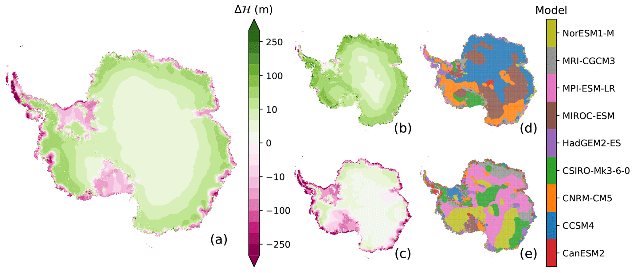
Figure 10Ice thickness changes since 1850 under the RCP8.5 scenario for applied precipitation anomalies in the year 2200. The ensemble mean (a), ensemble maximum (b), and ensemble minimum (c) are highlighted. The climate models that were used to drive the ice sheet model simulation causing the maximum and minimum thickness are shown in panels (d) and (e), respectively, next to the ensemble maximum (b) and minimum (c).
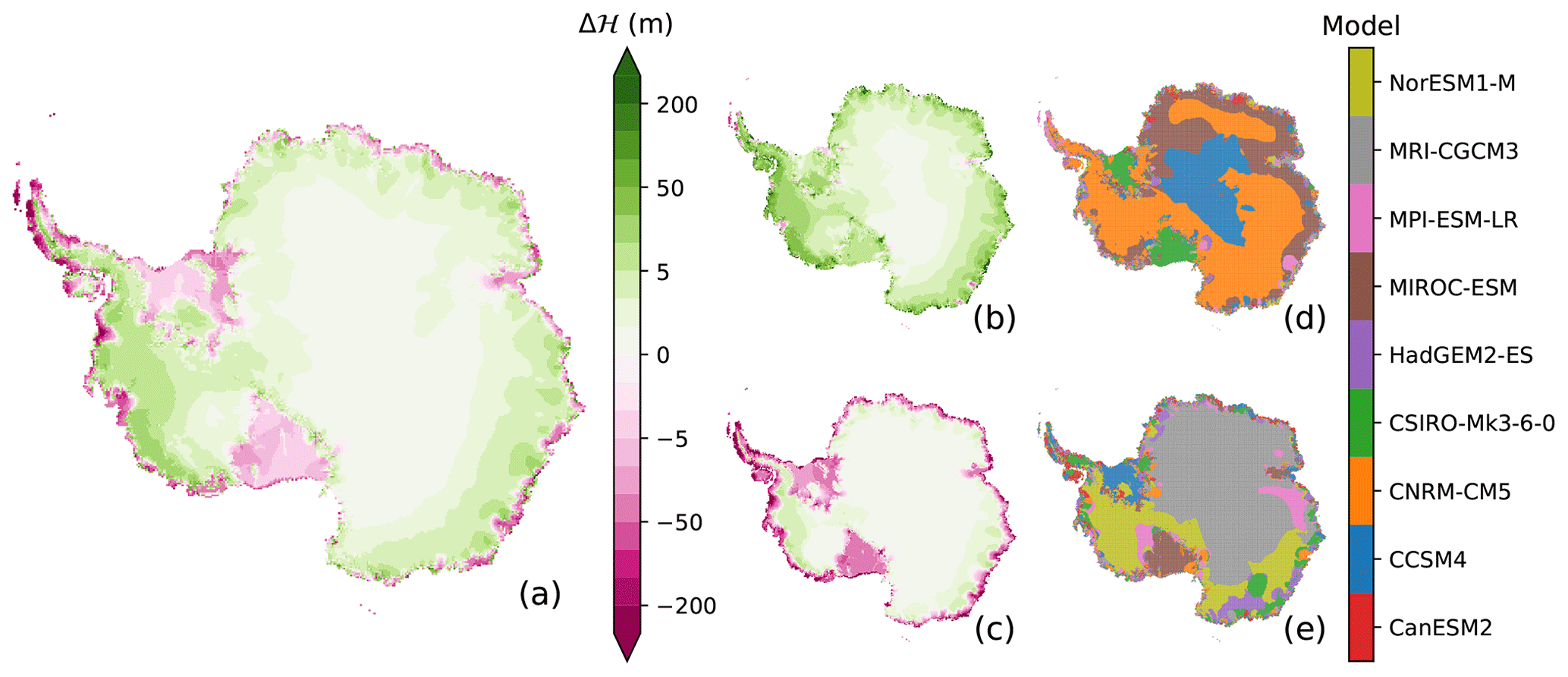
Figure 11Ice thickness changes since the year 1850 under the RCP8.5 scenario in the model year 2100. Here the precipitation is scaled by the air temperature anomaly with a value of 5 % K−1. The ensemble mean (a), ensemble maximum (b), and ensemble minimum (c) are depicted. The climate models that were used to drive the ice sheet model simulation causing the maximum and minimum thickness are shown in panels (d) and (e), respectively, next to the ensemble maximum (b) and minimum (c). This figure is similar to Fig. 9, but Fig. 9 shows the results under precipitation anomalies.
For grounded ice, three models (CCSM4, CNRM-CM5, and MIROC-ESM) predominantly determine the growing ice until the year 2100 (Fig. 9d), which is in line with the diagnosed sea level contribution (solid line, Fig. 6a, b). CCSM4 dominates the “EAIS Atl” sector, whereas CNRM-CM5 dominates a band from the “EAIS Ind” sector clockwise to the Antarctica Peninsula, which is interrupted by regional-scale patches of the MIROC-ESM model. A spatial dominance is not apparent for the minimum ice thickness, because the patchwork of five models (CSIRO-Mk3-6-0, HadGEM2-ES, MPI-ESM-LR, MRI-CGCM3, and NorESM1-M) dominates the year 2100. NorESM1-M influences the WAIS, which is supported by its lowest scaling in the Siple Coast region (Fig. 5); CSIRO-Mk3-6-0 has an impact around the South Pole; and MRI-CGCM3 affects the coastal zone in the EAIS. The control of MPI-ESM-LR and, to a lesser extent, HadGEM2-ES spreads across the entire continent. If we progress into the year 2200, where we have applied the 30-year forcing more than three times, the emerging picture is nearly unchanged for the maximum thicknesses. In contrast, the diversity in the models causing minimum thicknesses shrinks and is apparently dominated by CSIRO-Mk3-6-0, NorESM1-M, and MPI-ESM-LR (Fig. 10).
4.1.2 Ice sheet simulations driven by air-temperature-scaled precipitation
We now turn towards those model simulations in which the air-temperature-scaled precipitation forcing has been applied. In these simulations, the mean, maximum, and minimum ice thickness distributions (Fig. 11) are similar to those driven by the precipitation anomalies as discussed above (Fig. 7). Moreover, the same models determine the ice shelf thickness of the Filchner–Ronne and Ross ice shelves. The latter shows that the ocean primarily controls ice shelf thickness changes in our simulations. However, we detect a stark contrast in the models determining the maximum and minimum ice thickness. For the maximum, we still have the same three models (CCSM4, CNRM-CM5, and MIROC-ESM); however, the pattern has changed. CCSM4 controls a smaller area in the interior around the South Pole, and MIROC-ESM controls some coastal regions of the East Antarctic continent. The remaining majority of the grounded ice is under the control of CNRM-CM5. The most striking changes occur for the minimum. Now, NorESM1-M determines the entire WAIS and also some parts of “EAIS Ind”; MRI-CGCM3 dominates the remaining East Antarctic Ice Sheet.
In the latter case, air temperature variations exclusively force the precipitation-driven ice sheet thickness evolution (see Eq. 1). Dynamical changes influencing the precipitation are not considered. Hence, the scaling or precipitation boundary condition applied impacts the temporal evolution of the Antarctic Ice Sheet geometry, which ultimately shapes Antarctica's contribution to the global sea level.
4.2 Ice sheet losses
After the spin-up, the simulations reached a quasi-equilibrium. For the discussion of the ice losses, we concentrate on the transient period from 1850 to 2100 (Fig. 12. For all climate scenarios, the calving rate hardly changes (Fig. E12), whereas the total ice shelf area is nearly constant until 2000 and declines afterward (Fig. E15). The ocean-driven basal melting is proportional to the squared ocean temperature difference between the pressure-dependent melting temperature and the actual ocean temperature. As the ocean temperature increases in general (Figs. 2f, i, l, 3c), the mass loss by basal melting also increases, while the total shelf ice area remains quasi-constant until 2000 and declines afterwards (Fig. E15). For RCP8.5, the basal melting increases at the end of the 21st century quadratically. To conclude, the calving rate is nearly constant, whereas the basal melting increases by approximately 33 % between 2000 and 2100.
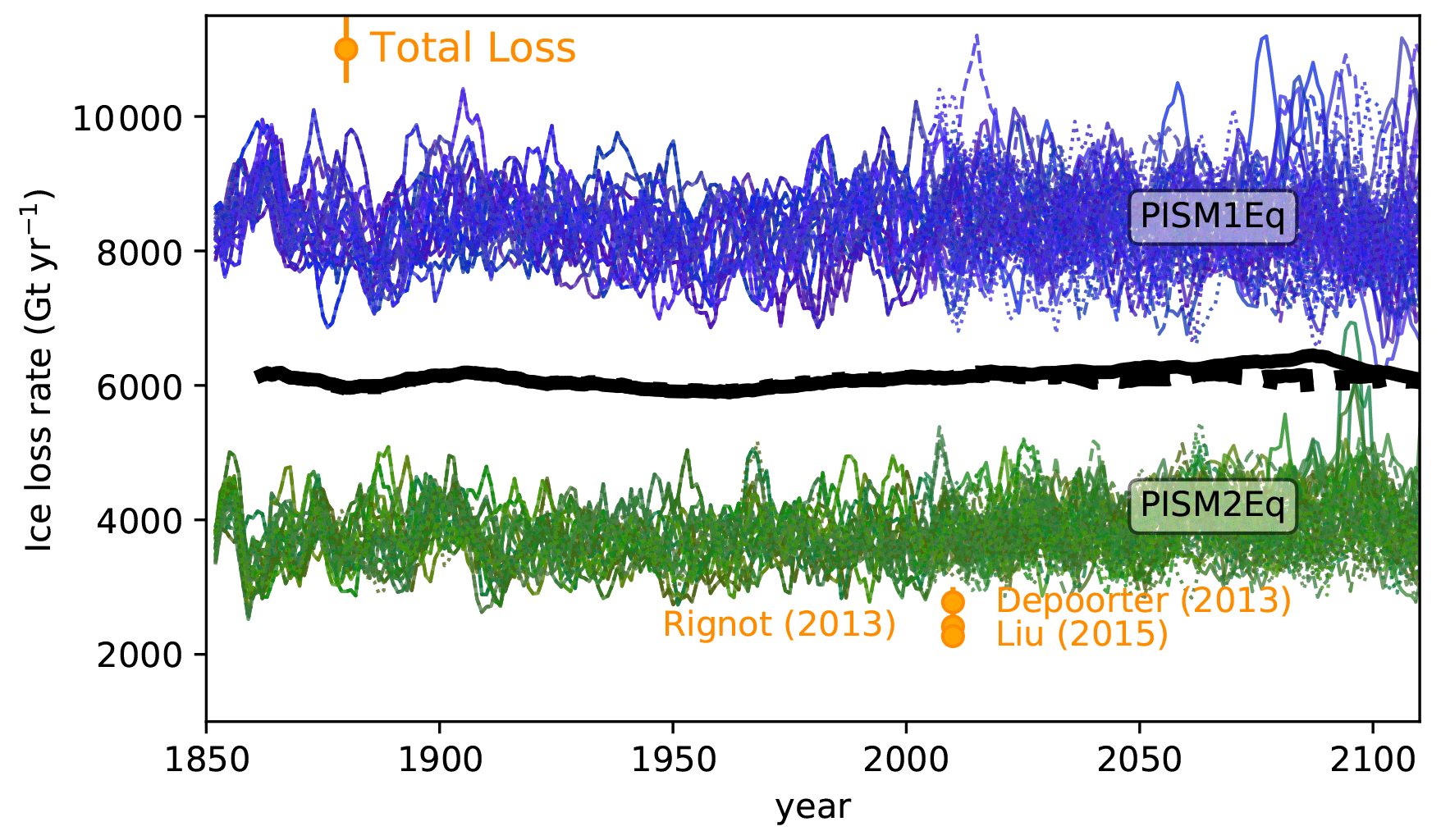
Figure 12Temporal evolution of the ocean-driven ice loss rates of the ice shelves around Antarctica for the period from 1850 to 2100. The ice loss comprises iceberg discharge and basal melting of ice shelves. The thin blue lines are all ensemble members starting from the PISM1Eq initial state, where the Eigen-calving parameter amounts to 1018; the green lines are the corresponding simulations starting from PISM2Eq (Eigen-calving parameter of 1017). A running mean with a window of 5 years has been applied for the thin lines. All simulations start under historical conditions and continue after 2005 under the RCP8.5 (solid lines), RCP4.5 (dashed lines), or RCP2.6 (dotted lines) scenarios. The thick black lines represent the ensemble mean of the three future scenarios with a moving window length of 25 years. Recent estimates of the total loss rates (top-left legend with the golden circles). Estimated uncertainties are given as vertical lines if the uncertainties are larger than the symbol size.
The mean calving rate is about 8000 and 5000 Gt yr−1 for the ensemble member utilizing the parameters and the PISM1Eq and PISM2Eq initial states, respectively (Fig. E12). The basal melting rates for PISM1Eq and PISM2Eq are similar; however, the loss rates for PISM1Eq are slightly larger than PISM2Eq (Fig. E13). The ensemble mean starts at about 550 Gt yr−1 in 1850 and reaches 900 Gt yr−1 in 2100.
As floating ice shelves nourish ice losses by basal ice shelf melting and iceberg calving, these ice losses do not directly impact the sea level. Under the assumption that the inflow of former grounded ice compensates for any shelf mass loss, the reported ice losses of 8500–9000 Gt yr−1 (5500–6000 Gt yr−1) would correspond to a sea level rise of 2.58–2.74 cm yr1 (1.67–1.83 cm yr1). The integration over 250 years to match the period from 1850 to 2100 would generate a potential sea level equivalent of 6.47–6.85 m (4.19–4.57 m). However, the actual ratio between total ice mass change and the corresponding potential sea level response is obviously not a 1:1 relation. Instead, on average, less than 5 % of the total mass lost diminishes grounded ice that raises the sea level (Fig. E8). Considering this ratio of 5 %, the sea level impact decreases to 0.32–0.34 m (0.21–0.23 m) by 2100. This is less than integrated precipitation anomalies across the Antarctic continent (Fig. 6a), which explains the total mass gains.
Nevertheless, the integrated basal melting rates are too low (Fig. E13) and the calving rates are too high (Fig. E12) compared with observational estimates in our ensemble of ice sheet model simulations. Besides the fact that the total loss exceeds recent observational estimates (Fig. 12), our ice sheet is in a quasi-equilibrium after the spin-up. All of this may indicate that the integrated precipitation-driven accumulation resulting from the RACMO precipitation reference field might be too large. However, the surface mass balance of RACMO agrees well with observational estimates (Wang et al., 2016), while the uncertainty of the surface mass balance (sea level equivalent of ∼0.25 mm yr−1 (Van Wessem et al., 2014)) is almost the same size as Antarctica's observation-based sea level contribution (∼0.2 mm yr−1 between 1992 and 2011; Shepherd et al., 2012; Wang et al., 2016). Additionally, recent satellite-based estimates clearly indicate that the Antarctic Ice Sheet has lost mass (sea level equivalent of 0.4 mm yr−1) in the period from 2011 to 2017 (Sasgen et al., 2019).
Beyond the year 2100 (Fig. E14), the calving rates decrease and reach a minimum in the period from 3000 to 4000. Afterward, calving increases again slightly. Basal melting rates are subject to a slight decreasing trend (RCP2.6), nearly constant values (RCP4.5), or a negligible upward trend after the year 4000 (RCP8.5).
4.2.1 Sea level contribution of corrected basal melting
As the simulated sea level contribution of Antarctica disagrees with the currently observed state showing mass loss, we apply a corrected time series emulating the observation-based ocean-driven basal melting. The purpose of this analysis is to reveal if a more vibrant basal melting rate, in concert with the simulated ice sheet mass evolution, leads to less pronounced ice sheet growth or perhaps even drives ice loss. Ultimately, we wish to establish if more vigorous melting of ice shelves raises the simulated sea level of all ensemble members?
By construction, the corrected time series preserve the fluxes' amplification over time, which is essentially the ratio of the higher end value to the lower start value. Hence, the corrected basal melt flux replicates the original simulated amplification, and the flux is identical to the observed reference value (Fref(tref)) at the reference time (tref). Under the assumption that only a fraction of the adjusted basal mass contributes to the global sea level, we apply the simulated ratio of the sea level change to the total ice mass change. This ratio renders the so-called dynamic ice loss, and it is the median ratio over its entire time series for each ensemble member (see Sect. D for details). As we examine enhanced mass loss, we do not adjust the iceberg calving rates that are already higher than observed values.
By adjusting the basal melting flux, the determined temporal evolution of the sea level correction (Fig. E5, Eq. D8) does impact the global simulated sea level. Still, it does not change the sign of the contemporary sea level evolution. Consequently, the impact on the simulated sea level is very small (Fig. E6). If we instead assume that all of the additional mass loss of floating ice shelves increases the simulated sea level immediately, we would obtain overly extensive corrections of 30 cm between 1850 and 2000. This corresponding sea level rise would be larger than the observed integrated sea level rise of about 20 cm since 1850 (Church and White, 2011), which has been driven by worldwide land-water storage changes, shrinking glaciers around the globe, enhanced melting from Greenland, and thermal expansion of the ocean (Cazenave and Remy, 2011; Leclercq et al., 2011; Church and White, 2011).
The sea level correction exceeds observations considerably under the unrealistic assumption that additional basal melting of already floating ice shelves would immediately raise the sea level. In contrast, a negligible sea level correction occurs if we apply the inferred ratio of about 5 % between simulated total ice mass loss and the corresponding sea level rise. In summary, a more vigorous but realistic melting of ice shelves does not essentially increase the simulated sea level.
4.3 Limitations
The simulations presented here are in contrast to others that project a sea level rise from a shrinking Antarctic Ice Sheet. Some previous studies have simulated Antarctica with a finer spatial resolution (Golledge et al., 2015; Pollard et al., 2015), which could improve the representation of ice streams. These streams channelize the flow of grounded ice from the interior to the margins, where they feed the attached ice shelves and discharge directly into the ocean. Despite our coarser resolution than those used in recent studies, our simulated surface velocity distribution reasonably reproduces satellite-based estimates (Figs. E10, E11). Others used the cliff failure parameterization that supports ice loss along with a constant ocean temperature offset of +2 ∘C (Pollard et al., 2015), which is twice as large as the amount found in our data set of nine CMIP5 models (Fig. 3), or they utilized continuously increasing atmospheric and oceanographic temperature forcing (Golledge et al., 2015; Mengel et al., 2015; Winkelmann et al., 2012, 2015) beyond the year 2100. These stronger forcings alone explain a large part of the difference, because we recurrently apply the forcing of the years from 2071 to 2100 after 2100.
As already discussed, the application of anomalies may trigger a small shock at the beginning of each simulation. This shock creates an initial artificial trend in the simulated sea level time series. Nevertheless, the long-term positive and negative sea level contribution of Antarctica for simulations driven by respective temperature-scaled and directly applied precipitation anomalies are robust.
The parameterization of the grounding line migration could be an issue, because a high resolution of about 1–2 km is needed according to Gladstone et al. (2012). However, medium- to lower-resolution grounding line parameterizations in PISM are consistent with higher-order models (Feldmann et al., 2014). This explains that the present-day grounding line position resembles the current state reasonably, and the simulated grounding line retreat follows the bulk of simulations in the last model intercomparison (Seroussi et al., 2019a); hence, we consider our grounding line migration to be reasonable. The apparent stability of ice shelves in the runs driven by the precipitation anomalies seems to comply with the safety band of ice shelves (Fürst et al., 2016), so the calving stays outside of ice shelf regions essential for providing buttressing for the inflowing grounded ice streams.
The ocean boundary condition, where ocean conditions are extrapolated into the ice shelf cavities, drive basal ablation of ice shelves. Here, we could undoubtedly improve simulations if the ice shelves were coupled to the driving ocean model, so that basal melting impacts the thermal structure of the ocean and, ultimately, the melt patterns. CMIP5 models neglect the ocean–ice-shelf interaction (Meijers, 2014), and their coarse resolution around Antarctica does not allow for the representation of the regional conditions (Heuzé et al., 2013; Sallée et al., 2013b). They are subject to unrealistic open-ocean convection (Heuzé et al., 2013; Meijers, 2014; Sallée et al., 2013a) instead of convection on or near the continental shelf (Årthun et al., 2013; Nicholls et al., 2009). All of these taint the hydrographic structure along Antarctica's coasts. Hence, any improved parameterization can not rectify the existing biases in the ocean forcing. These biases are reduced if we apply ocean temperature anomalies on top of an observation-based climatological data set, as performed in our study.
As we extrapolate coastal ocean temperatures laterally into the ice shelf cavities, the ocean warming obtained might be higher if it included the amplified warming of the gyre centers. Whether or not this was incorporated in the forcing of other groups obtaining a higher ice loss depends on the setup details. However, it may help to bridge the gap between other studies and our simulations.
Nevertheless, the simulated sea level decrease for the precipitation anomaly forcing used is in agreement with a growing surface mass balance since 1800, mainly driven by the Antarctic Peninsula region (Thomas et al., 2017). During intensive El Nino years, the accumulation-driven ice height increase between Dotson Ice Shelf and Ross Ice Shelf exceeds the height reduction by basal melting processes (Paolo et al., 2018), but the ice mass is still decreasing, as low-density snowfall replaces ice with a higher density. The stability arguments of Ritz et al. (2015) confirm the apparent stability of Antarctica in our simulations. Furthermore, various recent ice sheet model simulations, driven by selected CMIP5 climate model fields in the framework of the ISMIP6 exercise, are subject to a negative sea level contribution under a warming climate (Seroussi et al., 2019b).
How precipitation is specified in ice sheet simulations is crucial to the outcome of numerical simulations of Antarctica's sea level contribution. The commonly used method of scaling the precipitation changes with the simulated air temperature changes from ice cores or global climate models leads to a positive Antarctic simulated sea level contribution, i.e., a simulated sea level rise. However, when considering the simulated precipitation changes from the global climate models, the situation changes. In this case, our numerical projections simulate a negative sea level contribution. Nevertheless, independent of the precipitation boundary condition applied, we detect regions where the ice sheet thickness thins for all ensemble members. These regions are the Amundsen Sea embayment including Pine Island and Thwaites glaciers, some outlet glaciers of the East Antarctic Ice Sheet (EAIS) between George V and Wilkes Land, the Amery Ice Shelf, and along the Northern Antarctic Peninsula (Fig. 7c, e). These regions correspond to areas that have been identified across 16 models within a recent model intercomparison exercise, where marginal ice wanes due to ocean warming (Seroussi et al., 2019a).
Precipitation and air temperature, on average over the entire Antarctic continent, grow simultaneously in climate model simulations of the future (Fig. 3). In concert with estimates of accumulation changes and air temperature anomalies obtained from ice cores, this may (mis)lead us to scale the precipitation by the temporally evolving air temperature. Therefore, fixed scaling factors are common. However, a tendency towards higher scaling exists under more vigorous climate trends (Fig. 5), and the scaling has a clear spatial dependence (Figs. 4, 5). As a consequence, the accumulated snowfall on Antarctica for future climate projections differs between methods, which ultimately leads to biased estimates of Antarctica's contribution to the global potential sea level (Fig. 6). To assess the introduced bias, we analyze simulations of the Parallel Ice Sheet Model driven with numerous variants of the abovementioned climate conditions and a diverse set of implemented boundary conditions.
The “Siple Coast” region (area 0.69×10⁶ km2, see Table 5) as a part of the “WAIS” region (area 4.26×10⁶ km2) is different in many aspects. It has the smallest area compared with the other regions (Table 5), and it shows the lowest mean scaling factors for all scenarios. Moreover, as shown previously, no clear trend exists between different scenarios across the entire CMIP5 data set, whereas the spread of trends among individual CMIP5 models is substantial (Fig. 5). Furthermore, some members exhibit a negative scaling, where precipitation decreases for rising air temperatures: MPI-ESM-LR under the RCP8.5 scenario and NorESM1-M under all scenarios (RCP8.5, RCP4.5, and RCP2.6). Observations over the last few decades feature a downward trend in snow accumulation in this region (Wang et al., 2017). The inverted sign of the scaling is in stark contrast to the CMIP6 data set average.
Major uncertainties affect these simulations, such as the partitioning of ice losses into calving and basal melt – which is quite different from observational estimates due to very crude representations in the ice sheet model – or the omission of important processes, such as the interaction between the ocean, ice shelves, and ice sheets. While we could improve some aspects of the involved process descriptions, our simulations are state of the art and, therefore, suffer from the same limitations as others.
As the precipitation boundary condition determines if Antarctica raises or lowers the global sea level (Fig. 8), it may be appropriate to utilize a more sophisticated surface mass balance (SMB) model. The recent publication that indicates a “Greenlandification” of Antarctica's margin at the end of the century (Bell et al., 2018) supports this approach, but the required atmospheric inputs fields are not available at a sufficient temporal resolution. Hence, this will be an option for simulations driven by the forthcoming CMIP6 model output.
To evaluate the impact of the precipitation boundary condition, fully coupled simulations between a dynamic ice-sheet–ice-shelf model and a global climate model are inevitable. The system would include the ice-shelf–ocean interaction of coupled ocean–ice shelves at a sufficiently high spatial resolution around Antarctica. In addition, it would contain a sophisticated surface mass balance computation. We hope that these coupled atmosphere–ocean–sea-ice–ice-sheet–ice-shelf models will overcome the abovementioned limitations. The discrepancy in the simulation results between both methods describing the precipitation illustrates the uncertainty of the possible range of future precipitation growth in a warming world.
Regarding oceanic influence, we focus on the changes in the mean potential ocean temperature under the RCP8.5 scenario at a depth of between 150 and 500 m (Fig. 3), because these water masses flow into the ice sheet cavities and are in contact with the ice shelves' bases. The highest ocean temperature increases occur in the Bellingshausen and the Amundsen seas as part of the West Antarctic Ice Sheet (WAIS) and some locations along the East Antarctic Ice Sheet (EAIS) according to observations (Schmidtko et al., 2014; Jacobs, 2006). In the Bellingshausen and the Amundsen seas, warm water masses flow into ice shelf cavities, as indicated by observations (Arneborg et al., 2012; Thompson et al., 2018) and model simulations (Nakayama et al., 2018). These water masses drive the highest basal melting rates (Nakayama et al., 2014) that trigger potential marine ice sheet instability (MISI) because the WAIS has a retrograde bedrock topography. The tremendous Filchner–Ronne, Ross, and Amery ice shelves are influenced by moderate ocean temperature increases. However, our setup misses the interaction between the ice shelf topography and the underlying dynamically evolving ocean. Hence, the setup does not describe related circulation changes that may bring warmer water masses into the ice cavities. For instance, it has been found that warmer water masses could find their way into these ice shelf cavities and cause a strongly amplified basal mass loss under a changing climate (Hellmer et al., 2012). They have simulated an ocean warming of more then 2 ∘C in the Filchner Trough (eastern Filchner–Ronne Ice Shelf). At the terminus of the Filchner–Ronne Ice Shelf, our CMIP5 data set maximum ocean temperature anomaly (Fig. E1) of about 1.5 ∘C generates a much weaker forcing.
If one calculates temperature scaling factors out of the CMIP5 model simulated air temperature and precipitation changes, it turns out that the temperature scaling factor of the precipitation is different for each model and, therefore, shows an inhomogeneous spatial pattern (Fig. E3). Furthermore, the details of the scaling factors depend on the time period that we chose as a reference, which drives our ice sheet simulations, relative to the first or last 50 years of the corresponding piControl runs. If we alternatively compute the anomalies relative to the averaged first 30 years of the historical period (1850–1879), we also obtain slightly different results. However, these differences do not significantly change the spatial structure. The choice of the baseline (first or last 50 years of piControl or first 30 years of the historical period) to compute the scaling distribution is of minor consequence. However, selecting the forcing data set from the pool of CMIP5 models overwhelmingly determines the scaling distribution. The scaling factors averaged across Antarctica reveal that the scatter range for one model is much smaller than the scaling values' distance among models (Fig. 5).
The scaling across all model tends to be highest for the EAIS, where the part facing the Atlantic Ocean exhibits the highest scalings (Fig. 5). The WAIS has a lower scaling, and the embedded “Siple Coast” region has the lowest scaling on average. There is a tendency for a higher scaling under a more vigorously changing climate across all regions, except for the smallest region “Ross”. This tendency exists for the CMIP5 data set average and across models characterized by a larger than average scaling. Most models represent the detected precipitation deficit (shrinking precipitation rates), captured by reanalysis data and shallow ice cores in the “Siple Coast” region (Wang et al., 2017). Only NorESM1-M reproduces less precipitation (precipitation deficit) under rising air temperatures across all future climate scenarios. When considering the whole of Antarctica, the difference between the grounded ice sheet only and all glaciated regions (including ice shelves) is small.
MIROC-ESM has the highest scaling spread between the first and last 50 years of the piControl reference period across all of the inspected regions and scenarios (see the scatter range in Fig. 5), which is probably related to the pronounced trend of the global 2 m air temperature (0.67 ∘C) between these two reference periods in our CMIP5 data set. Otherwise, the spread is related to enhanced or amplified long-term regional climate variability expressed by differing values in the reference period. For example, CCSM4 or MPI-ESM-LR is subject to a larger spread in the Atlantic sector of the EAIS, whereas the variability is negligible in the neighboring Indian sector. The higher spread of the smaller Ross subregion within the WAIS sector supports this interpretation (at least for the CCSM4, CanESM2, and HadGEM2-ESM models).
A tendency exists towards a higher scaling of coastal areas that are subject to incoming storm tracks, which potentially deliver heavier precipitation events that are also controlled by the rising topography height towards the interior of Antarctica. In the majority of the simulations, we identify a lower scaling in WAIS as well as a low to negative scaling in the area of the Ross Ice Shelf and the adjacent parts of the WAIS.
We turn our analysis to the individual mass balance terms: iceberg calving, basal melting in the ice shelf cavities, and surface mass balance. To recap, the surface mass balance is obtained by applying the individual spatial atmospheric model forcing on top of the reference fields obtained from RACMO, whereas the basal melting is calculated by adding ocean anomalies on top of the World Ocean Atlas climatology (Table 2). The calving is composed of three processes (thickness calving, Eigen-calving, and kill mask calving) as part of the Parallel Ice Sheet Model (PISM) simulations. Here, the analysis focuses predominantly on the period from 1850 to 2100, because we reapply the forcing from 2071–2100 recurrently after 2100.
Until 2100, the temporal evolution of the iceberg calving rates of individual ensemble members is subject to some variability, which is typical for such event-based mass losses. For some models, we could identify some reduced calving of 20 % around 1850 and 1970 as well as some enhanced calving of 25 % around 1920 and 2050. For individual ensemble members, the temporal evolution of the calving rate is noisy and independent of the forcing scenario applied: RCP2.6, RCP4.5, and RCP8.5 (Fig. E12). Overall, the temporal evolution of the calving does not show a clear trend, and the average calving loss rate of the entire ensemble is about 5500 Gt yr−1 (Fig. E12). The calving rates of ensemble members starting from the PISM1Eq or PISM2Eq initial states are clearly separated. The members of the group starting from PISM1Eq have an average calving rate of approximately 7500 Gt yr−1, whereas the average rate is about 3500 Gt yr−1 for PISM2Eq. Thus, a reduction in the Eigen-calving constant by an order of magnitude from 1018 (PISM1Eq) to 1017 (PISM2Eq) approximately halves the total calving rate, and the thickness calving is active for a marginal ice shelf point with a thickness of less than 150 m in both cases.
According to observational estimates, iceberg calving and basal ice shelf melting control the overall mass loss of Antarctica, although the relative contribution of each is the subject of current research. Depoorter et al. (2013) reported a nearly equal share between calving (1321±144 Gt yr−1) and basal melting (1454±174 Gt yr−1) in the period between 1995 and 2009; Rignot et al. (2013) detected a slightly higher contribution from basal melting (1325±235 Gt yr−1 compared with calving with 1089±139 Gt yr−1) between 2003 and 2008; and Liu et al. (2015) found that the basal melting (1516±106 Gt yr−1) contribution was twice as much as the calving (755±24 Gt yr−1) contribution (2005–2011).
Both ensemble branches starting from PISM1Eq and PISM2Eq overestimate the currently observed calving rates of less than 1500 Gt yr−1 (Depoorter et al., 2013; Liu et al., 2015; Rignot et al., 2013). Moreover, the combined observed mass loss from calving and basal melting of ice shelves, which is about 2500 Gt yr−1 (Depoorter et al., 2013; Liu et al., 2015; Rignot et al., 2013), is smaller on average than the lower simulated calving rate from our ensemble members starting from PISM2Eq. Therefore, our ensemble mean ice loss rate exceeds current estimates, which could lead to an overestimation of the total sea level rise in our simulations.
The basal melting rate of floating ice shelves (hereinafter basal melting rates) is the second ocean-driven ice mass loss process beside iceberg calving. In broad terms, the basal melt rate generally increases by 10 %–100 % over the period from 1850 to 2100 (Fig. E13). Initially, the melting rises slowly because the additional ocean temperature forcing remains weak (Fig. 3). Starting around the year 1970, the increase becomes nonlinear and basal melting accelerates. The simulated historical trend is nearly independent of the initial state (PISM1Eq and PISM2Eq) and the reference period selected for the computation of the ocean temperature anomaly. For each climate model scenario, the anomalies are computed relative to the first or last 50 years of the preindustrial climate (piControl) simulations. However, the reference state only matters for MIROC-ESM (first vs. last 50 years of piControl), because this model is subject to a non-negligible trend (0.08 m) during the piControl phase. For instance, the average of the global absolute 2 m air temperature difference between the first and last 50 years of piControl amount to 0.17 K (median 0.12 K) for all CMIP5 models considered in our study. In contrast, the value from MIROC-ESM is 0.67 K.
In future projections, the basal melting rate increases by between 10 % and more than 100 % until the year 2100 relative to the 50-year reference period from 1951 to 2000. The latter increase is consistent with results from dedicated ocean simulations. These simulations resolve ice shelves, explicitly including the ocean–ice-sheet interaction, and are driven by future projection from various climate models (Naughten et al., 2018; Hellmer et al., 2012).
The basal melting rates increase until 2100 but then suddenly decrease back to 2071 values (Fig. E13); this is due to the fact that, by experimental design, the last 30 years of forcing (2071–2100) is repeated after the year 2100. Furthermore, the separation of ensemble members starting from PISM1Eq and PISM2Eq is self-evident for the basal melting. However, both groups are close to the ensemble mean, which is in contrast to the calving rate. The basal melting rates of all ensemble members underestimate the observed basal melting rates.
As the observed calving rate is generally lower than the basal melting rate, our model ensemble swaps the importance of basal melting and iceberg calving. Moreover, the sum of the calving rate and basal melting rate exceeds the observed estimates. Hence, our simulations could tend to overestimate ice loss and, ultimately, sea level rise.
The ensemble mean calving and basal melting rates remain almost constant or reach a maximum in around 2100, and scenarios with a higher forcing (RCP8.5 vs. RCP4.5, for instance) cause more ice loss due to both calving and basal melting. Beyond 2100, ice loss rates decrease in general (Fig. E14). As the temporal variability also remains high after 2100, our approach works to construct the forcing beyond the year 2100 (see Sect. 2). To highlight the primary trend in the temporal evolution after 2100, a 250-year running mean is applied after 2100.
The basal melting rates of the stronger forcing scenario (RCP8.5) show a minimum around the year 3500 and increase slightly afterward, whereas the other scenarios (RCP4.5 and RCP2.6) indicate a tendency towards stabilization at the end of our simulation in the year 5000 (Fig. E14). Over the entire period, the basal melting rate is higher for the stronger forcing scenarios. This result reflects the dependence of the basal melting on the ocean temperature, because a warmer climate scenario induces higher ocean temperature anomalies.
The calving rates before 2100 tend to be slightly higher for the RCP8.5 scenario. However, after 2100, we detect the sharpest drop in the ice loss rates for the scenario RCP8.5, an intermediate decrement for RCP4.5, and a moderate reduction for RCP2.6 (Fig. E14). Around 3000, RCP8.5 calving reaches its minimum, followed by an enhanced increase for 500 years and a moderate increase afterward. Scenarios with reduced radiative forcing reach a minimum later: RCP4.5 reaches a minimum around 3200, whereas RCP2.6 reaches a minimum around 3700. At this time, the ensemble mean calving rates of RCP4.5 and RCP2.6 are similar (note that RCP2.6 does not include simulations driven by CCSM4). The trends of all scenarios converge around 4000.
In the long term, the most active basal melting is seen under the stronger forcing scenarios, whereas the highest calving occurs under scenarios with a lower forcing. The calving rate controls the evolution of the total ice mass loss in our simulations. Before the year 2100, RCP8.5 has the highest calving rates, whereas these are lowest shortly afterward. After 2100, the ensemble members showing the highest calving rates are driven by the low-end scenario (RCP2.6). The ensemble mean of the basal melting increases by 60 %–70 %, 70 %–85 %, and 90 %–115 %, for RCP2.6, RCP4.5, and RCP8.5, respectively. The fractional calving change in the ensemble mean is between +2 % and −4 %, between +2 % and −10 %, and between +2 % and −19 % for RCP2.6, RCP4.5, and RCP8.5, respectively. Across these scenarios, we detect that the most substantial ice shelf area reduction occurs for RCP8.5 and the lowest reduction occurs for RCP2.6. Our simulations suggest that the warmer climate causes a stronger ice shelf retreat and a stronger drop in the calving rate during the period in which the ice shelf could adjust to the quasi-equilibrium forcing. Based on these results, we conclude that a warmer climate drives more basal melting and enhances calving so that we obtain smaller ice shelves. The total area of ice shelves is generally smaller when a warmer climate scenario impacts them (Fig. E15), and the degraded total ice shelf area downgrades the calving probability. Ultimately, the integrated calving rate is lower under a warmer climate.
As the simulated ocean-driven basal melting rates are lower than observation-based estimates (Fig. E13), the impact of flux-corrected basal melting rates on the model results are discussed in the main text (Sect. 4.2.1). This section describes the method.
Starting from original simulated ablation flux Forg, which could be the basal melting flux or the iceberg discharge flux , and the corresponding reference flux Fref(tref) at time tref, we define the following ratios: the fraction of the temporally evolving flux (Forg(t)) to the original flux at the reference time (tref),
and the fraction of the original simulated flux to the reference flux (Fref),
The corrected flux Fcor using Eq. (D1) is defined as
so that the flux difference ΔF(t) is
With Eq. (D2) we obtain
To relate the sea level change to the ice mass evolution, we define the ratio p(t) of the sea level temporal deviation to the ice mass temporal deviation as follows:
where zl is the sea level, and mice is the total ice mass, which includes grounded and floating ice. Here, we use p=median(p(t)) so that each ensemble member is characterized by one value for its entire time series. If , 100 % of the flux difference (Eq. D4) contributes immediately to the sea level of the global ocean with an area of Aoce.
The total ice mass (mice) changes are driven by four terms
where FSMB(t) is the surface mass balance flux, and FG(t) is the basal mass flux of grounded ice (Fig. E9). We assume that these two terms in the brackets do not change regardless of the corrections applied to the last two terms FB and FD. Hence, the difference in the ice mass change is
Now we relate the temporal evolution of the sea level to the total ice mass changes by utilizing Eq. (D5),
so that we obtain
where the sea level difference Δzl(t) is
Figures E5 and E7 depict the sea level difference for two cases. If the additional mass loss immediately contributes to a rising sea level (Fig. E7), the corresponding sea level rise of 30 cm would be larger than the actual sea level rise since 1850 of about 20 cm (Church and White, 2011). This case is not realistic, because a melting floating ice shelf does not impact the sea level. Only the flow of grounded ice across the grounding line, to feed an ice shelf, or the direct loss of grounded ice contributes to the sea level.
In contrast, the sea level hardly changes (Fig. E5) if the deduced ratio , which corresponds to the ratio defined in Equation D5. This is computed for each ensemble mean as the median of its time series. Whether the ratio between ice loss and sea level rise is constant under amplified basal melting of ice shelves or not is an open question. Strongly intensified ocean-driven ice loss will probably cause a retreating grounding line on a longer timescale, which ultimately releases grounded ice into the sea and increases the sea level.
Figure E8 shows the proportion of the deduced ratio to the 100 % ratio. Only very few ensemble member lose about 15 % of the maximum value of . In contrast, the mean and median value of this proportion is generally less then 5 %. For all ensemble members driven by the precipitation anomaly, this proportion is 4.7 % on average with a median of 3.9 %. It is even lower for ensemble members driven by the temperature-scaled precipitation. The median amounts to 0.7 %, and the corresponding mean is 0.9 %. Note that some ensemble members under the temperature-scaled precipitation are subject to a negative scaling. This result confirms the abovementioned low positive and negative scaling seen for restricted regions (Fig. 5). It also highlights that simulations driven by temperature-scaled precipitation could show unexpected results.
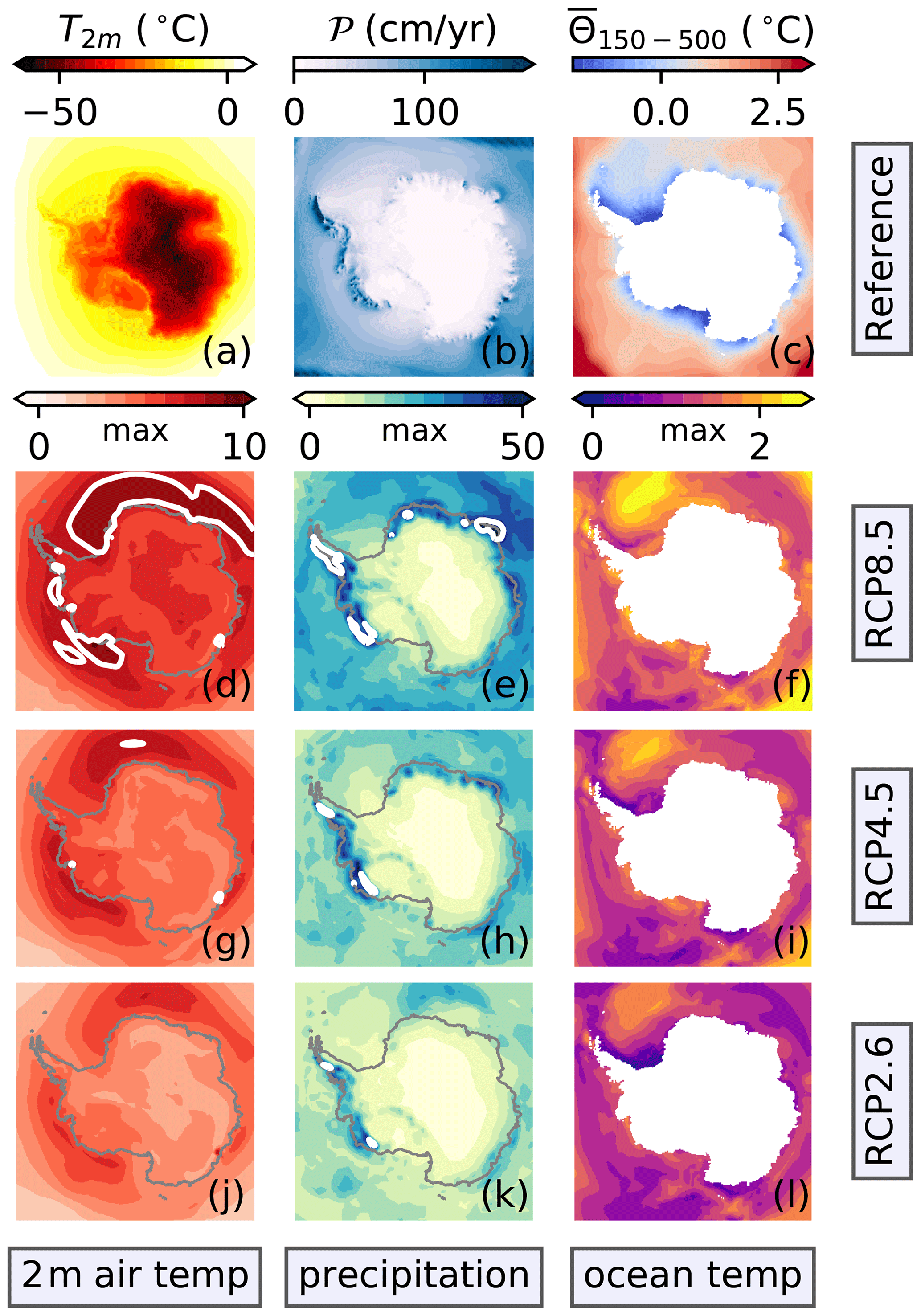
Figure E1CMIP5 data set maximum anomalies (d–l) relative to the atmospheric (a, b) and oceanographic (c) reference forcing. The corresponding mean and minimum fields are depicted in Figs. 2 and E2, respectively. Panels (a–c) represent the reference fields to spin-up the ice sheet model (Table 2). The 2 m air temperature (a) and the total precipitation (b) are mean fields from the regional RACMO model, and the ocean temperatures are from the World Ocean Atlas 2009 (c). Below each reference field, the related maximum anomalies are compiled for the period from 2071 to 2100. Here, panels (d–f), (g–i), and (j–l) show the anomalies for RCP8.5, RCP4.5, and RCP2.6, respectively. The dark-gray line follows the current coastline. All potential ocean temperatures (c, f, i, l) are a vertical mean of the depth interval from 150 to 500 m. The white contour lines in the anomaly plots highlight the 2 m air temperature threshold (d, g, j) of 8 ∘C and the total precipitation threshold (e, h, k) of 50 cm yr−1. All of these anomalies are the CMIP5 data set maximum of the models listed in Table 1; CCSM4 is not part of RCP2.6.
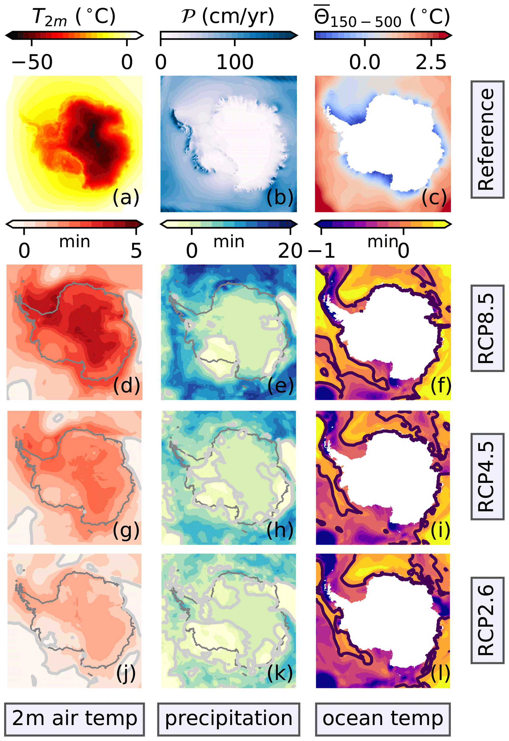
Figure E2CMIP5 data set minimum anomalies (d–l) relative to the atmospheric (a, b) and oceanographic (c) reference forcing. The corresponding mean and maximum fields are depicted in Figs. 2 and E1, respectively. Panels (a–c) represent the reference fields to spin-up the ice sheet model (Table 2). The 2 m air temperature (a) and the total precipitation (b) are mean fields from the regional RACMO model, and the ocean temperatures are from the World Ocean Atlas 2009 (c). Below each reference field, the related minimum anomalies are compiled for the period from 2071 to 2100. Here, panels (d–f), (g–i), and (j–l) show the anomalies for RCP8.5, RCP4.5, and RCP2.6, respectively. The dark-gray line follows the current coastline. All potential ocean temperatures (c, f, i, l) are vertical means of the depth interval from 150 to 500 m. The light-gray lines in the anomaly plots highlight the 2 m air temperature threshold (d, g, j) of 0 ∘C, the total precipitation threshold (e, h, k) of 0 cm yr−1, and the potential ocean temperature threshold (f, i, l) of 0 ∘C. All of these anomalies are the CMIP5 data set minimum of the models listed in Table 1; CCSM4 is not part of RCP2.6.
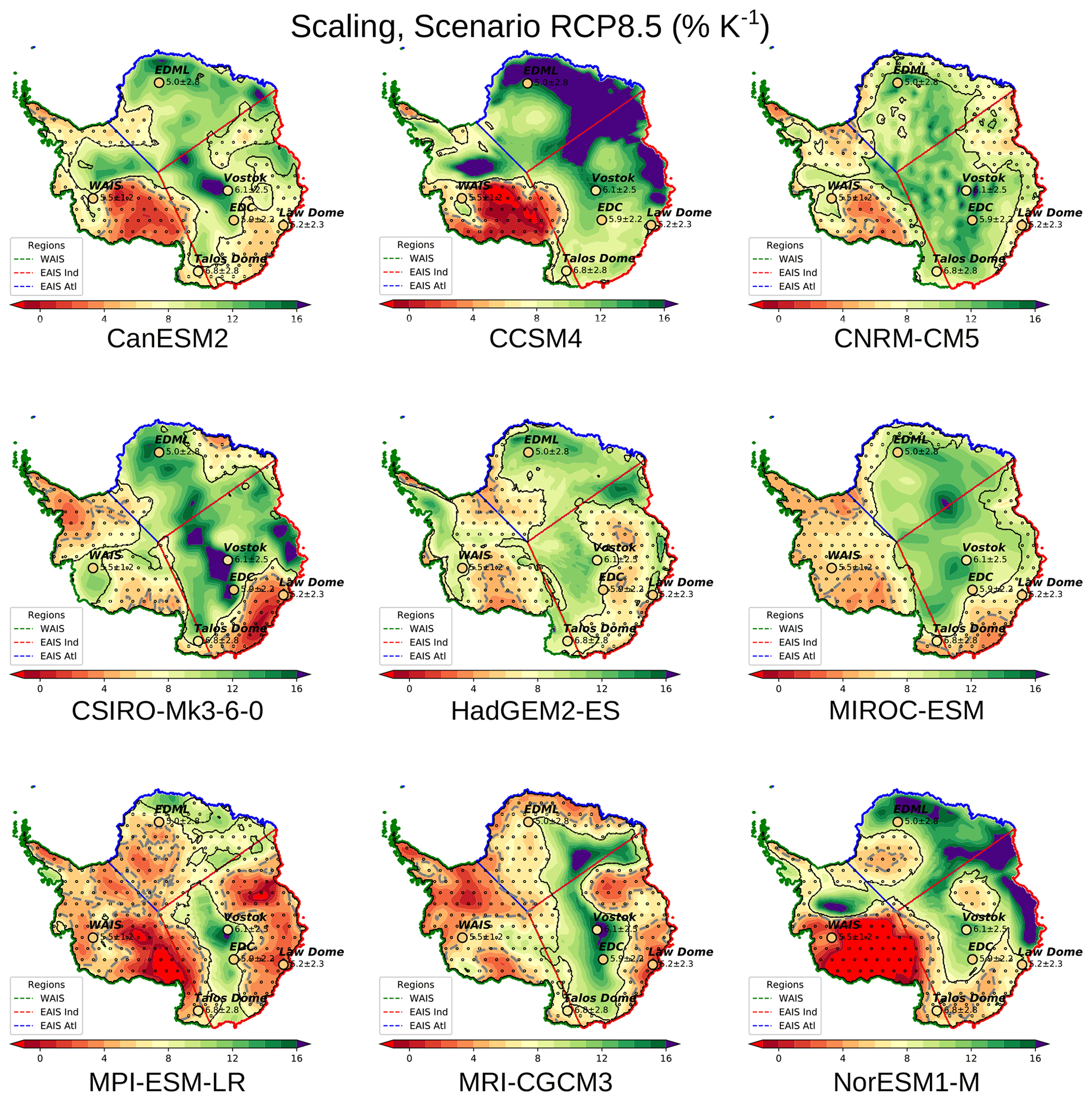
Figure E3Air-temperature-scaled precipitation under the RCP8.5 scenario for nine CMIP5 models (Table 1) for the period from 2051 to 2100. The ice sheet simulations are driven by anomalies relative to the first 50 years of the related piControl climate scenario. In the dotted regions enclosed by black contours, the combined simulated scaling and the standard deviation contain the value of 5 % K−1. Gray dashed lines follow this 5 % K−1 contour. The scaling values deduced from ice cores are shown at their location (mean and the 2σ uncertainty). The “WAIS,” “EAIS Atl,” and “EAIS Ind” region boundaries are outlined in green, blue, and red, respectively (lower left legend). For further details, the reader is referred to Sect. 3.2. Figure 4 shows the corresponding CMIP5 data set average. The contours of the Antarctic continent are deduced from Fretwell et al. (2013).

Figure E4Integrated potential sea level equivalent of the precipitation falling on Antarctica (see the inset mask in each subpanel) from the anomaly forcing (a, b: solid lines) and temperature-scaled precipitation (a, b: dashed lines). The potential sea level impact between the anomalies and the temperature-scaled precipitation (c, d) is depicted for each CMIP5 model. The left and right columns show the results under the RCP4.5 and RCP8.5 scenarios, respectively. The upper row depicts the scaling for the entire Antarctic continent (“glaciered”), whereas the lower row is restricted to grounded ice. The lower left set of subpanels is identical to Fig. 6. The reader is referred to Fig. 6 for further details. The grounded and floating ice areas are derived from Fretwell et al. (2013).
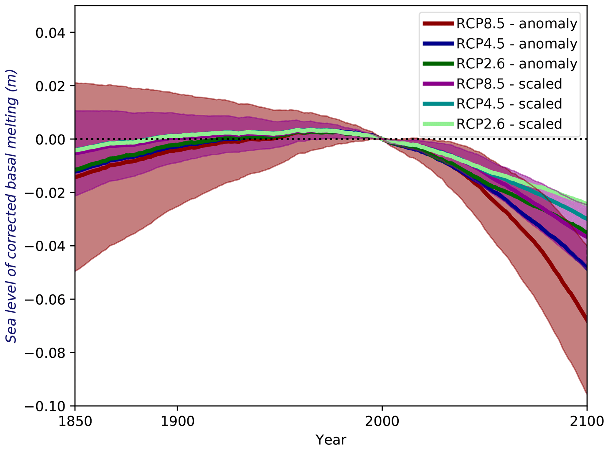
Figure E5The sea level correction as defined by Eq. (D8) covers the period from 1850 to 2100. Here, the ratio p(t) (Eq. D5) is the temporal median for each ensemble member (see Fig. E7 for the corresponding figure assuming that all additional mass loss increases the global simulated sea level). The correction is computed relative to the simulated sea level for each individual simulation for the year 2000 as in Fig. 8. The resulting simulated sea level for the entire period from 1850 to 5000 is depicted in Fig. E6. We use 1431 Gt yr−1 as a reference value for the basal melting rate ; this value corresponds to the estimate of Depoorter et al. (2013) of 1454±174 Gt yr−1, whereas it falls below the value of 1516±106 Gt yr−1 observed by Liu et al. (2015) and exceeds the rate of 1325±235 Gt yr−1 reported by Rignot et al. (2013). Our reference corresponds to the mean of all of these basal melting estimates: 1431 Gt yr−1.
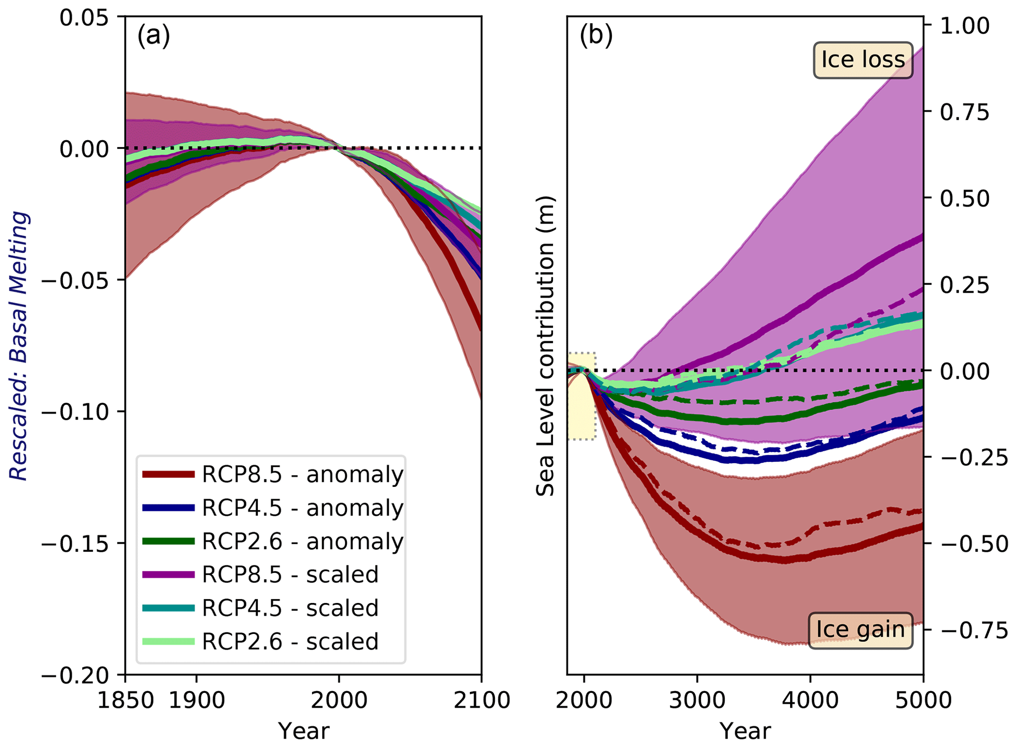
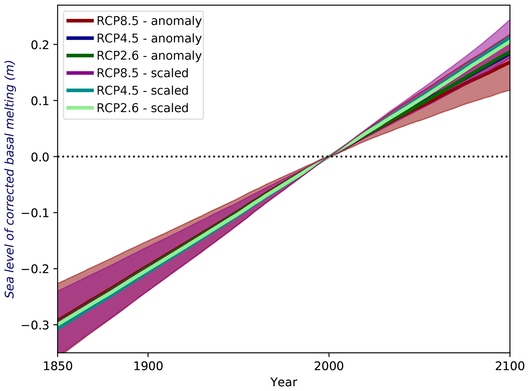
Figure E7The sea level correction as defined by Eq. (D8) covers the period from 1850 to 2100, where 100 % of the additional mass loss contributes immediately to a rising sea level; hence, the ratio p (Eq. D5) equals . The correction is computed relative to the simulated sea level for each individual simulation at the year 2000 as in Fig. 8. The corresponding Fig. E5 depicts the case where the correction considers the actual deduced ratio p(t).
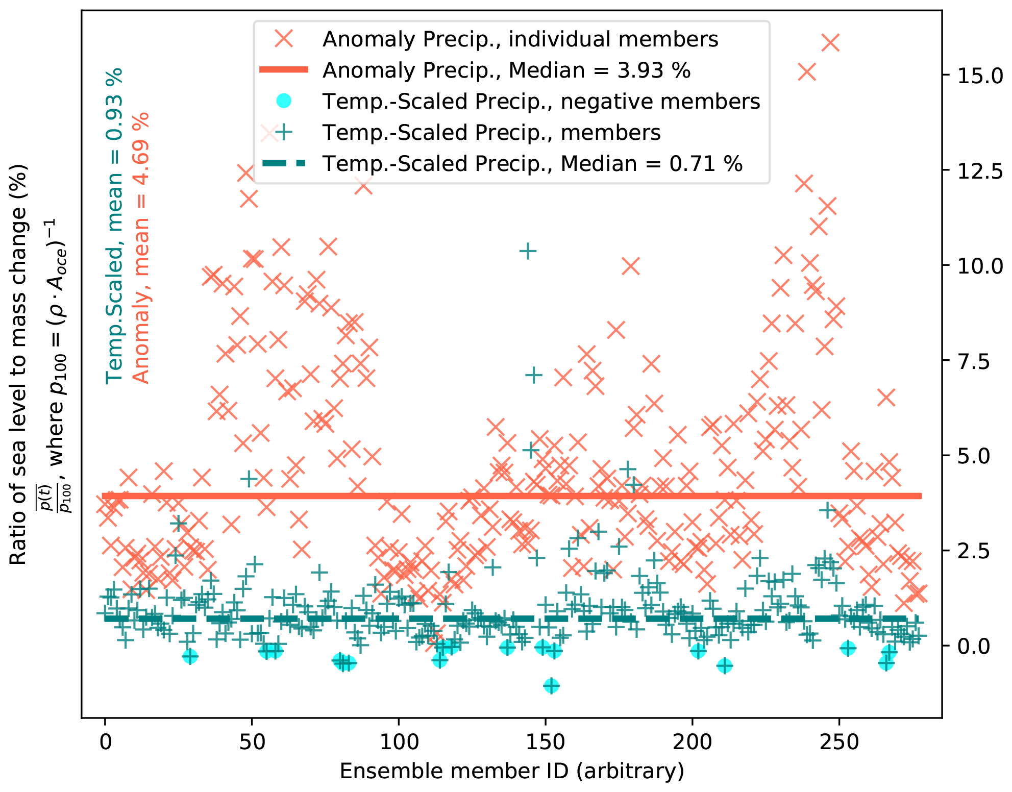
Figure E8The ratio between the actual sea level contribution due to mass loss and the sea level equivalent of corresponding mass. Individual ensemble members are shown as crosses. A red “x” represents a member that is driven by the precipitation anomaly, and a blue-green “+” indicates those driven by the temperature-scaled precipitation. In the latter case, light-blue circles highlight members with negative ratios. Vertical lines mark median values for these two groups (see the legend). The corresponding mean values are listed on the left. The term is defined by Eq. (D5) and , where ρ is the density and Aoce represents the global ocean area.
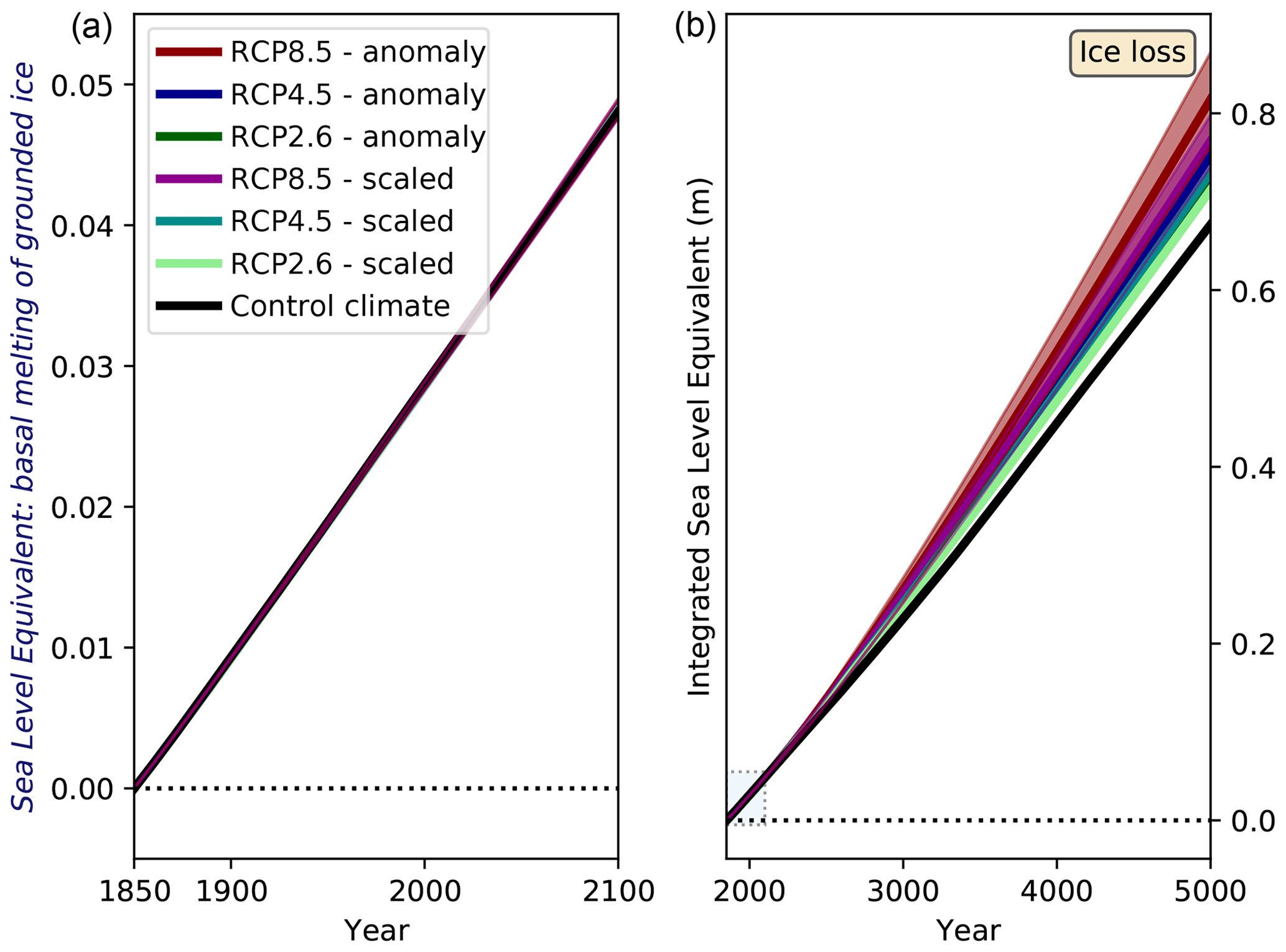
Figure E9Cumulated basal melting of grounded ice as sea level equivalent. The results of the entire ensemble of ice sheet simulations are shown. The solid lines represent the ensemble averages for the applied precipitation anomalies and the temperature-scaled precipitation boundary conditions according to the legend. For the RCP8.5 scenario, the shading highlights the standard deviation (1σ) as a measure of the variability among the ice sheet ensemble members driven by various climate models (Table 1).
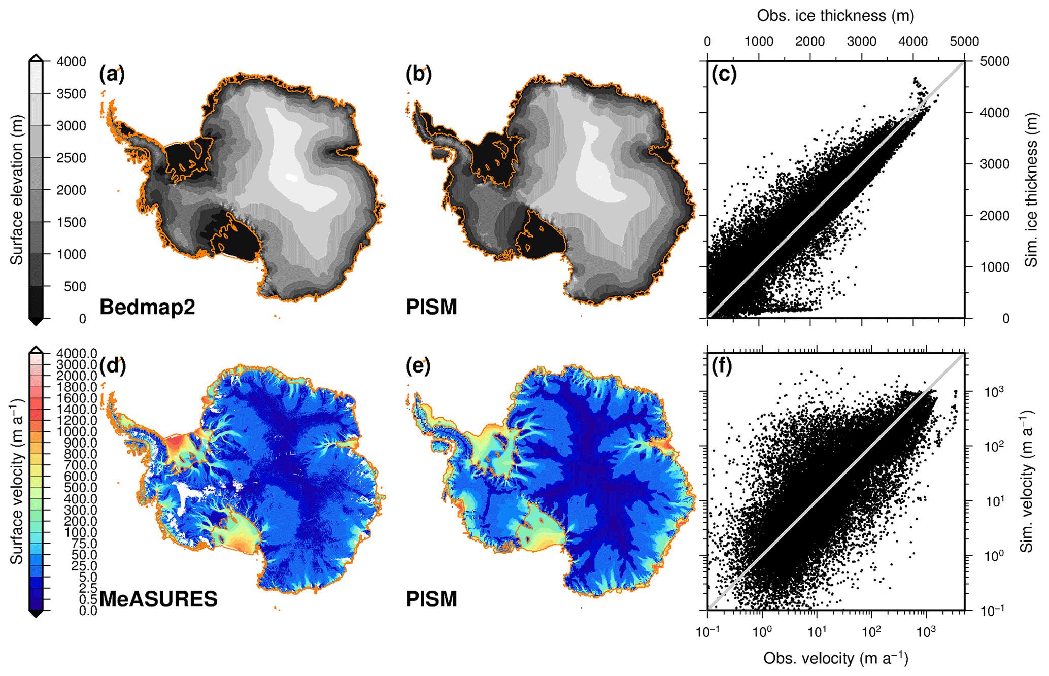
Figure E10Comparison between the initial state PISM1Eq and observational estimates. Panels (a–c) depict the surface elevation using (a) the Bedmap2 data set (Fretwell et al., 2013), (b) the simulated ice elevation in PISM, and (c) a point-wise comparison. Panels (d–f) show the surface velocity distribution using (d) observations (Rignot et al., 2016), (e) simulated values, and (f) a point-wise comparison; note that both axes are logarithmic. For the point-wise comparison, the observations follow the x axis (abscissa), and the simulated values follow the y axis (ordinate). Essential information about the initial ice-covered area and volume as well as its comparison with the other initial state PISM1Eq (Fig. E11) is listed in Table F1.
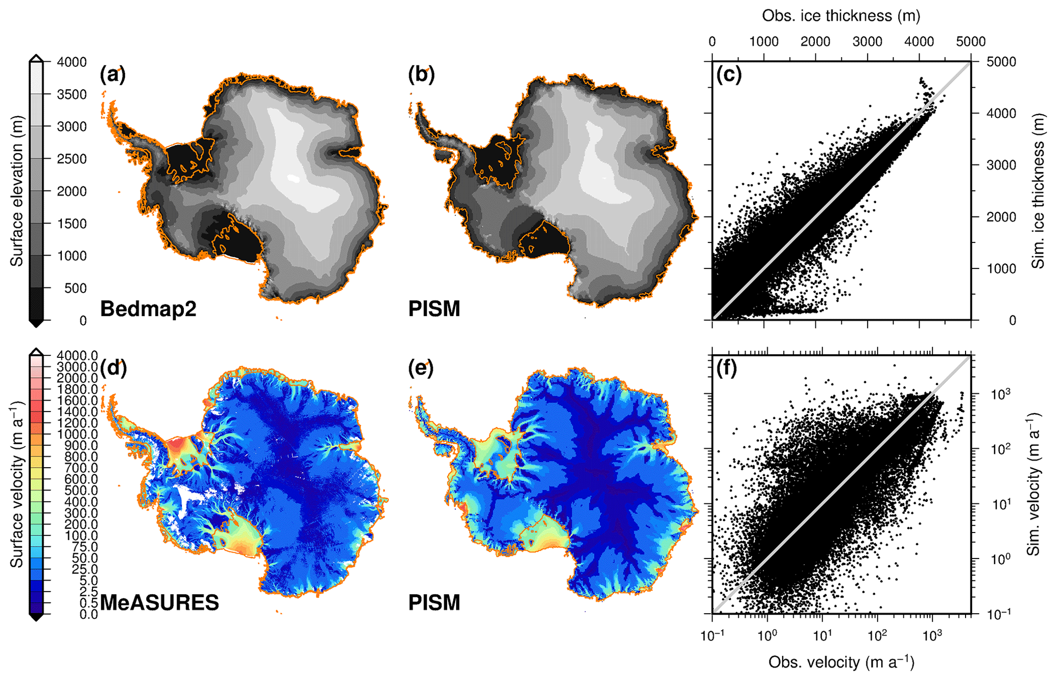
Figure E11Comparison between the initial state PISM2Eq and observational estimates. Panels (a–c) depict the surface elevation using (a) the Bedmap2 data set (Fretwell et al., 2013), (b) the elevation in PISM, and (c) a point-wise comparison. Panels (d–f) show the surface velocity using (d) observations (Rignot et al., 2016), (e) simulated values, and (f) a point-wise comparison. The reader is referred to Fig. E10 (PISM1Eq) for further details and to Table F1 for essential information and a comparison of both states.

Figure E12Temporal evolution of Antarctic-wide calving rates for the period from 1850 to 2100. All simulations start under historical conditions and continue after 2005 under the RCP8.5 (solid lines), RCP4.5 (dashed lines), or RCP2.6 (dotted lines) scenarios. After the year 2100, the forcing of the last 30 years until 2100 drives the model recurrently. The thin blue lines are all ensemble members starting from the PISM1Eq initial state, where the Eigen-calving parameter amounts 1018; the green lines are the corresponding simulations starting from PISM2Eq (Eigen-calving parameter 1017). A running mean with a 5-year window has been applied for the thin lines. The thick black lines represent the ensemble mean of the three future scenarios with a 25-year moving window. The applied running means shift the apparent maximum backward in time so that it occurs visually before the year 2100. Recent estimates of the total (orange circles) and the calving (red squares) ice mass loss are given for three studies (legend at the top). Vertical bars depict the reported uncertainties of the estimates from Liu et al. (2015), Depoorter et al. (2013), and Rignot et al. (2013).
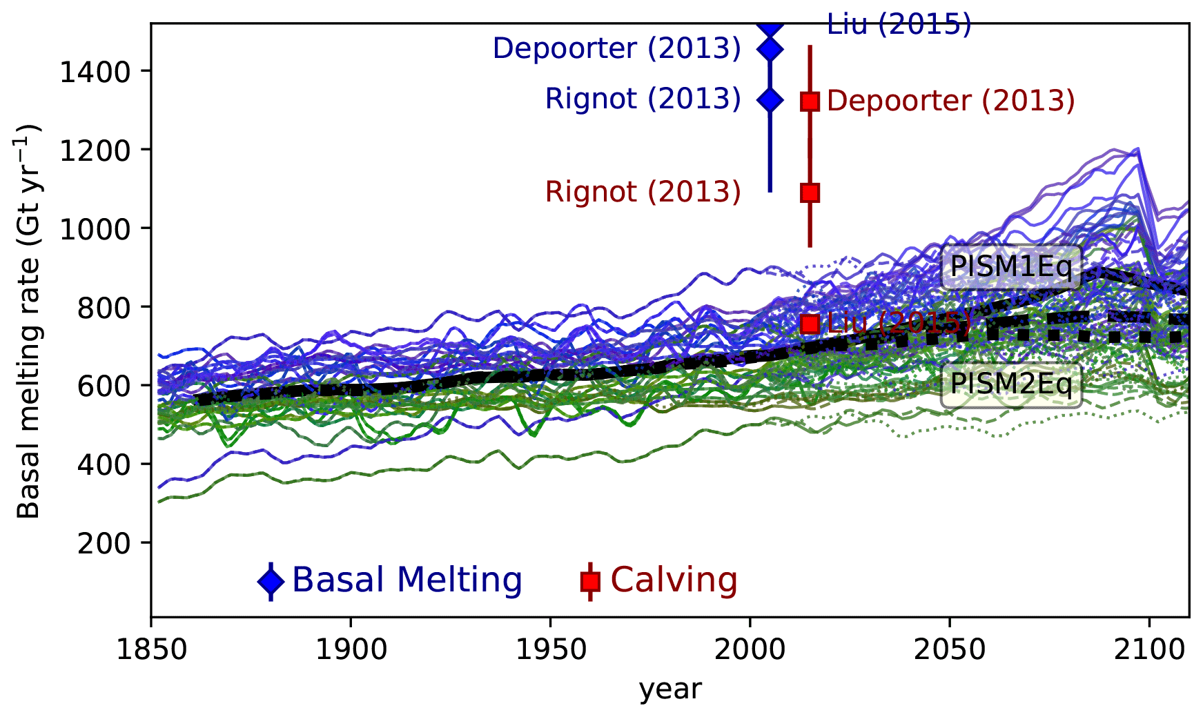
Figure E13Temporal evolution of the basal melting rates in ice shelves around Antarctica for the period from 1850 to 2100. All simulations start under historical conditions and continue after 2005 under the RCP8.5 (solid lines), RCP4.5 (dashed lines), or RCP2.6 (dotted lines) scenarios. After the year 2100, the forcing of the last 30 years until 2100 drives the model recurrently. The thin blue lines are all ensemble members starting from the PISM1Eq initial state, where the Eigen-calving parameter amounts 1018; the green lines are the corresponding simulations starting from PISM2Eq (Eigen-calving parameter 1017). A running mean with a 5-year window has been applied for the thin lines. The thick black lines represent the ensemble mean of the three future scenarios with a 25-year moving window. The applied running means shift the apparent maximum backward in time so that it occurs visually before the year 2100. Recent estimates of the basal melting (blue diamonds) and the calving (red squares) ice mass loss are given for three studies (legend at the bottom; Liu et al., 2015; Depoorter et al., 2013; Rignot et al., 2013). Related uncertainties are given as vertical lines if the uncertainties are larger than the symbol size.
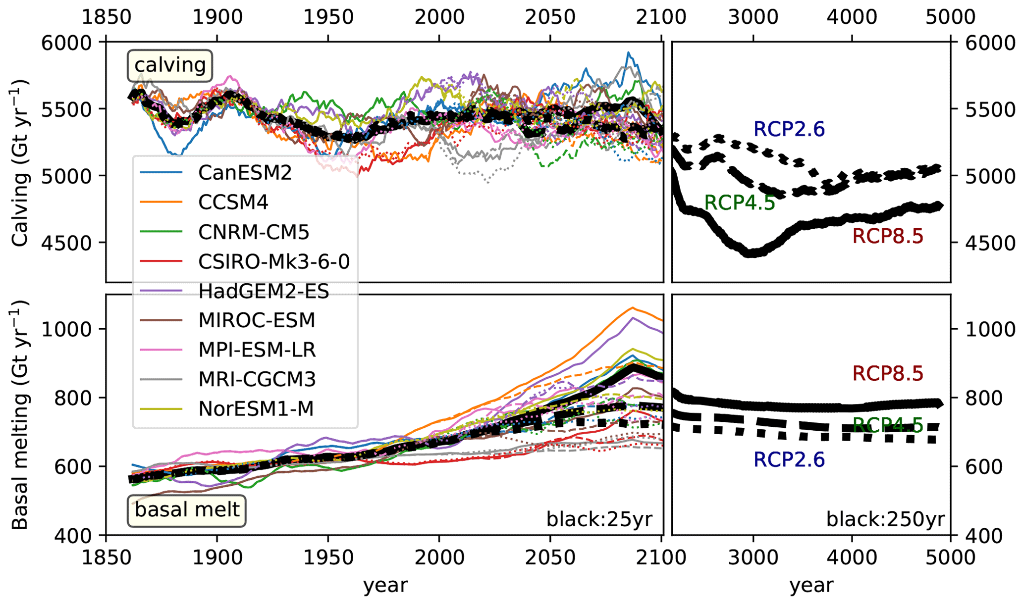
Figure E14Long-term temporal evolution of the ensemble mean basal melting and calving ice loss rates from 1850 to 2100 and beyond until the year 5000. The upper panels show the calving rates, and the lower panels depict the basal melting rates. In the left panels, individual model simulations (colored lines according to the legend) are grouped together, whereas the thick black lines are the overall means as shown in the corresponding figures (Figs. E12, E13). For the ensemble means of the period from 1850 to 2100, a smoothing with a 25-year moving window is applied (left panels), whereas the smoothing window length is 250 years for the right panels covering the period from 2100 to 5000. The applied running means shift the apparent maximum backward in time so that it occurs visually before the year 2100. Solid, dashed, and dotted lines represent the RCP8.5, RCP4.5, and RCP2.6 scenarios, respectively.
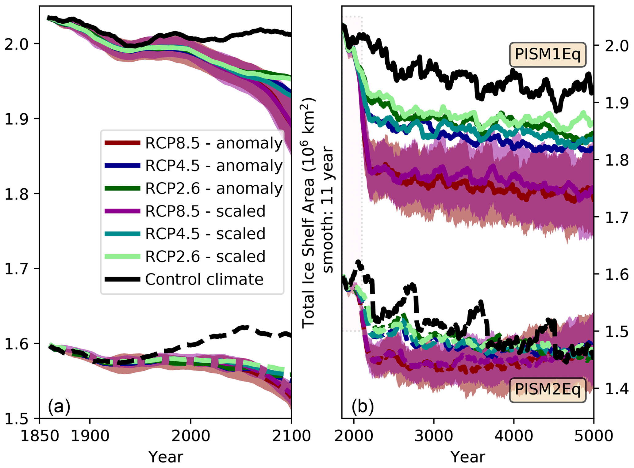
Figure E15Area of floating ice shelves. An 11-year running mean window is used for the entire ensemble of ice sheet simulations. The solid lines represent the ensemble averages for the PISM1Eq starting conditions, and the dashed lines are the corresponding PISM2Eq condition. For the RCP8.5 scenario, the shading highlights the standard deviation (1σ) as a measure of the variability among the ice sheet ensemble members driven by various climate models (Table 1). Note the different axes for both panes. The dashed frame in the right panel depicts the value range of the left panel.
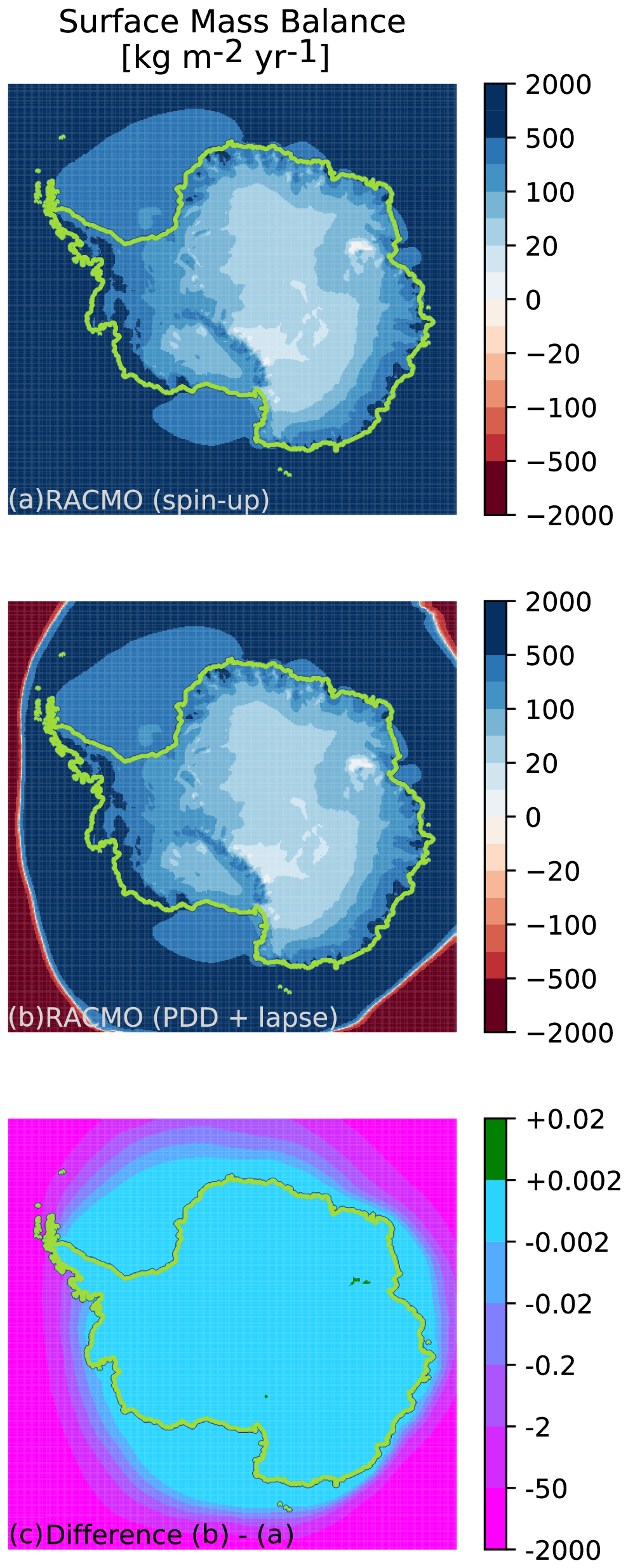
Figure E16Surface mass balance (SMB) used during the spin-up (a), the surface mass balance computed via the positive-degree-day (PDD) approach (b) under preindustrial conditions, and the difference between these (c). For the panel under preindustrial conditions (b), the lapse correction is also active, which does not impact the results because the height difference is initially neglectable. The unit of the surface mass balance and its difference are kilograms per square meter per year (kg m−2 yr−1); note that 1 kg m−2 yr−1 equals 1 mm(WE) yr−1 (WE represents water equivalent). In each subplot, the light-green contour lines represent the outer edge of the ice sheet or ice shelves, respectively. Approximately south of the annual sea ice edge, the difference between both SMB fields is essentially zero except for two restricted areas. One near the Amery Ice Shelf and the other at the Transantarctic mountain range east of the Ross Ice Shelf. These two regions are characterized by a negative SMB in the spin-up data distribution (a), which is absent in the PDD-deduced SMB (b). Moreover, only the northern tip of the Antarctic Peninsula experiences a different forcing. Further north, the difference is significant; however, this difference does not impact the Antarctic ice sheet.
Table F1Characteristics of both the PISM1Eq (Fig. E10) and PISM2Eq (Fig. E11) initial states. These are the total areas covered by grounded (Ag) and floating ice (Af). The table shows the volumes of all grounded ice (Vg), grounded ice above a sea level of z=0 (Vg0), and all floating ice (Vf). The bottom row presents the ratio, expressed as a percentage value, between grounded ice above the sea level and all grounded ice. The far right column represents the ratio of the quantities between both initial states.

The code of the Parallel Ice Sheet Model is freely available from https://github.com/pism/pism (last access: 22 November 2017) (The PISM Authors, 2015a, b). Modifications to the PISM's code are available from Thomas Kleiner upon reasonable request. The data are available from the corresponding author or Tido Semmler upon reasonable request.
MP and CBR prepared the CMIP5 data. CBR performed the simulations and wrote the article. All authors contributed to the interpretation of the results and proofreading of the paper.
The authors declare that they have no conflict of interest.
We thank all of the reviewers for their engagement and their excellent suggestions that helped to improve the paper. The Deutsches Klimarechenzentrum (DKRZ) supplied computer resources on the “Mistral” cluster. Christian B. Rodehacke wishes to thank the AWI's HPC administrators for their proactive and generous support that enabled this work during the development phase. Development of PISM is supported by NSF grant nos. PLR-1603799 and PLR-1644277 and NASA grant no. NNX17AG65G. The data analyses and the production of figures were predominantly performed with the help of the following software products (in alphabetic order): Climate Data Operators (CDO; https://code.mpimet.mpg.de/ projects/cdo, last access: 14 December 2020); Precipitation-dependent future sea level Generic Mapping Tools (GMT; https://www.generic-mapping-tools.org, last access: 14 December 2020); Ncview (http://meteora.ucsd.edu/~pierce/ncview_home_page.html, last access: 14 December 2020); netCDF Operator (NCO; http://nco.sourceforge.net, last access: 14 December 2020); PyFerret (https://ferret.pmel.noaa.gov/Ferret/documentation/pyferret, last access: 14 December 2020); and Python (Python 3, https://www.python.org, last access: 14 December 2020), including NumpPy (https://numpy.org, last access: 14 December 2020), matplotlib (https://matplotlib.org, last access: 14 December 2020), and xarray (https://xarray.pydata.org, last access: 14 December 2020). We thank the numerous authors and financial supporters of these software products.
This work has been financed through the German Federal Ministry of Education and Research (Bundesministerium für Bildung und Forschung: BMBF) project ZUWEISS (grant no. 01LS1612A). Parts of this work have been supported by BMBF grant no. 01LP1503B (project PalMod1.2). CBR acknowledges funding via the Alfred Wegener Institute's PACES2 research program.
The article processing charges for this open-access
publication were covered by a Research
Centre of the Helmholtz Association.
This paper was edited by Yun Liu and reviewed by Torsten Albrecht and two anonymous referees.
Adusumilli, S., Fricker, H. A., Siegfried, M. R., Padman, L., Paolo, F. S., and Ligtenberg, S. R. M.: Variable Basal Melt Rates of Antarctic Peninsula Ice Shelves, 1994–2016, Geophys. Res. Lett., 45, 4086–4095, https://doi.org/10.1002/2017GL076652, 2018. a
Agosta, C., Fettweis, X., and Datta, R.: Evaluation of the CMIP5 models in the aim of regional modelling of the Antarctic surface mass balance, The Cryosphere, 9, 2311–2321, https://doi.org/10.5194/tc-9-2311-2015, 2015. a
Allen, M. R. and Ingram, W. J.: Constraints on future changes in climate and the hydrologic cycle, Nature, 419, 228–232, https://doi.org/10.1038/nature01092, 2002. a
Applegate, P., Kirchner, N., Stone, E., Keller, K., and Greve, R.: An assessment of key model parametric uncertainties in projections of Greenland Ice Sheet behavior, The Cryosphere, 6, 589–606, https://doi.org/10.5194/tc-6-589-2012, 2012. a
Arneborg, L., Wåhlin, A., Björk, G., Liljebladh, B., and Orsi, A.: Persistent inflow of warm water onto the central Amundsen shelf, Nat. Geosci., 5, 876–880, https://doi.org/10.1038/ngeo1644, 2012. a
Årthun, M., Holland, P. R., Nicholls, K. W., and Feltham, D. L.: Eddy-Driven Exchange between the Open Ocean and a Sub–Ice Shelf Cavity, J. Phys. Oceanogr., 43, 2372–2387, https://doi.org/10.1175/JPO-D-13-0137.1, 2013. a
Bakker, P., Clark, P. U., Golledge, N. R., Schmittner, A., and Weber, M. E.: Centennial-scale Holocene climate variations amplified by Antarctic Ice Sheet discharge, Nature, 541, 72–76, https://doi.org/10.1038/nature20582, 2017. a
Banwell, A. F., MacAyeal, D. R., and Sergienko, O. V.: Break-up of the Larsen B Ice Shelf Triggered by Chain-Reaction Drainage of Supraglacial Lakes, Geophys. Res. Lett., 40, 5872–5876, https://doi.org/10.1002/2013GL057694, 2013. a
Banwell, A. F., Willis, I. C., Macdonald, G. J., Goodsell, B., and MacAyeal, D. R.: Direct measurements of ice-shelf flexure caused by surface meltwater ponding and drainage, Nat. Commun., 10, 730, https://doi.org/10.1038/s41467-019-08522-5, 2019. a
Bell, R. E., Chu, W., Kingslake, J., Das, I., Tedesco, M., Tinto, K. J., Zappa, C. J., Frezzotti, M., Boghosian, A., and Lee, W. S.: Antarctic ice shelf potentially stabilized by export of meltwater in surface river, Nature, 544, 344–348, https://doi.org/10.1038/nature22048, 2017. a
Bell, R. E., Banwell, A. F., Trusel, L. D., and Kingslake, J.: Antarctic surface hydrology and impacts on ice-sheet mass balance, Nat. Clim. Change, 8, 1044–1052, https://doi.org/10.1038/s41558-018-0326-3, 2018. a
Bintanja, R. and Selten, F.: Future increases in Arctic precipitation linked to local evaporation and sea-ice retreat, Nature, 509, 479–82, https://doi.org/10.1038/nature13259, 2014. a
Bracegirdle, T. J., Connolley, W. M., and Turner, J.: Antarctic climate change over the twenty first century, J. Geophys. Res., 113, D03103, https://doi.org/10.1029/2007JD008933, 2008. a, b
Bracegirdle, T. J., Stephenson, D. B., Turner, J., and Phillips, T.: The importance of sea ice area biases in 21st century multimodel projections of Antarctic temperature and precipitation, Geophys. Res. Lett., 42, 10832–10839, https://doi.org/10.1002/2015GL067055, 2015. a
Braithwaite, R. J.: Positive degree-day factors for ablation on the Greenland Ice-sheet studied by energy balance modeling, J. Glaciol., 41, 153–160, 1995. a
Bromwich, D. H., Nicolas, J. P., and Monaghan, A. J.: An Assessment of Precipitation Changes over Antarctica and the Southern Ocean since 1989 in Contemporary Global Reanalyses, J. Climate, 24, 4189–4209, https://doi.org/10.1175/2011JCLI4074.1, 2011. a, b
Bromwich, D. H., Nicolas, J. P., Monaghan, A. J., Lazzara, M. A., Keller, L. M., Weidner, G. A., and Wilson, A. B.: Central West Antarctica among the most rapidly warming regions on Earth, Nat. Geosci., 6, 139–145, https://doi.org/10.1038/ngeo1671, 2012. a
Bueler, E. and Brown, J.: Shallow shelf approximation as a “sliding law” in a thermomechanically coupled ice sheet model, J. Geophys. Res., 114, F03008, https://doi.org/10.1029/2008JF001179, 2009. a, b
Bueler, E., Lingle, C. S., and Brown, J.: Fast computation of a viscoelastic deformable Earth model for ice-sheet simulations, Ann. Glaciol., 46, 97–105, https://doi.org/10.3189/172756407782871567, 2007. a
Cazenave, A. and Remy, F.: Sea level and climate: measurements and causes of changes, Wiley Interdisciplin. Rev.: Clim. Change, 2, 647–662, https://doi.org/10.1002/wcc.139, 2011. a
Church, J. A. and White, N. J.: Sea-Level Rise from the Late 19th to the Early 21st Century, Surv. Geophys., 32, 585–602, https://doi.org/10.1007/s10712-011-9119-1, 2011. a, b, c
Church, J. A., White, N. J., Konikow, L. F., Domingues, C. M., Cogley, J. G., Rignot, E., Gregory, J. M., van den Broeke, M. R., Monaghan, A. J., and Velicogna, I.: Revisiting the Earth's sea-level and energy budgets from 1961 to 2008, Geophys. Res. Lett., 38, L18601, https://doi.org/10.1029/2011GL048794, 2011. a
Church, J., Clark, P., Cazenave, A., Gregory, J., Jevrejeva, S., Levermann, A., Merrifield, M., Milne, G., Nerem, R., Nunn, P., Payne, A., Pfeffer, W., Stammer, D., and Unnikrishnan, A.: Sea Level Change, in: Climate Change 2013: The Physical Science Basis. Contribution of Working Group I to the Fifth Assessment Report of the Intergovernmental Panel on Climate Change, chap. 13, edited by: Stocker, T., Qin, D., Plattner, G.-K., Tignor, M., Allen, S., Boschung, J., Nauels, A., Xia, Y., Bex, V., and Midgley, P., Cambridge University Press, Cambridge, UK and New York, NY, USA, available at: http://www.ipcc.ch/report/ar5/wg1/ (last access: 9 September 2019), 2013a. a
Church, J. A., White, N. J., Konikow, L. F., Domingues, C. M., Graham Cogley, J., Rignot, E., Gregory, J. M., van den Broeke, M. R., Monaghan, A. J., and Velicogna, I.: Correction to “Revisiting the Earth's sea-level and energy budgets from 1961 to 2008”, Geophys. Res. Lett., 40, 4066–4066, https://doi.org/10.1002/grl.50752, 2013b. a
Cook, A. J. and Vaughan, D. G.: Overview of areal changes of the ice shelves on the Antarctic Peninsula over the past 50 years, The Cryosphere, 4, 77–98, https://doi.org/10.5194/tc-4-77-2010, 2010. a
de Boer, B., van de Wal, R. S. W., Lourens, L. J., Bintanja, R., and Reerink, T. J.: A continuous simulation of global ice volume over the past 1 million years with 3-D ice-sheet models, Clim. Dynam., 41, 1365–1384, https://doi.org/10.1007/s00382-012-1562-2, 2013. a
Depoorter, M., Bamber, J., Griggs, J., Lenaerts, J., Ligtenberg, S., van den Broeke, M., and Moholdt, G.: Calving fluxes and basal melt rates of Antarctic ice shelves, Nature, 502, 89–92, https://doi.org/10.1038/nature12567, 2013. a, b, c, d, e, f, g, h, i
Doake, C.: Ice-shelf Stability, in: Encyclopedia of Ocean Sciences, edited by: Steele, J. H., Thorpe, S. A., and Turekian, K. K., January 1995, Elsevier, Amsterdam, 1282–1290, https://doi.org/10.1006/rwos.2001.0005, 2001. a
Eayrs, C., Holland, D., Francis, D., Wagner, T., Kumar, R., and Li, X.: Understanding the Seasonal Cycle of Antarctic Sea Ice Extent in the Context of Longer-Term Variability, Rev. Geophys., 57, 1037–1064, https://doi.org/10.1029/2018RG000631, 2019. a, b
Emori, S. and Brown, S. J.: Dynamic and thermodynamic changes in mean and extreme precipitation under changed climate, Geophys. Res. Lett., 32, 1–5, https://doi.org/10.1029/2005GL023272, 2005. a
Etourneau, J., Sgubin, G., Crosta, X., Swingedouw, D., Willmott, V., Barbara, L., Houssais, M.-N., Schouten, S., Damsté, J. S. S., Goosse, H., Escutia, C., Crespin, J., Massé, G., and Kim, J.-H.: Ocean temperature impact on ice shelf extent in the eastern Antarctic Peninsula, Nat. Commun., 10, 304, https://doi.org/10.1038/s41467-018-08195-6, 2019. a
Feldmann, J. and Levermann, A.: Collapse of the West Antarctic Ice Sheet after local destabilization of the Amundsen Basin, P. Natl. Acad. Sci. USA, 112, 14191–14196, https://doi.org/10.1073/pnas.1512482112, 2015. a
Feldmann, J., Albrecht, T., Khroulev, C., Pattyn, F., and Levermann, A.: Resolution-dependent performance of grounding line motion in a shallow model compared with a full-Stokes model according to the MISMIP3d intercomparison, J. Glaciol., 60, 353–360, https://doi.org/10.3189/2014JoG13J093, 2014. a, b
Flato, G., Marotzke, J., Abiodun, B., Braconnot, P., Chou, S., Collins, W., Cox, P., Driouech, F., Emori, S., Eyring, V., Forest, C., Gleckler, P., Guilyardi, E., Jakob, C., Kattsov, V., Reason, C., and Rummukainen, M.: Evaluation of Climate Models, in: Climate Change 2013: The Physical Science Basis, Contribution of Working Group I to the Fifth Assessment Report of the Intergovernmental Panel on Climate Change, chap. 9, edited by: Stocker, T., Qin, D., Plattner, G.-K., Tignor, M., Allen, S., Boschung, J., Nauels, A., Xia, Y., Bex, V., and Midgley, P., Cambridge University Press, Cambridge, UK and New York, NY, USA, 126 pp., available at: http://www.ipcc.ch/report/ar5/wg1/ (last access: 9 September 2019), 2013. a
Foldvik, A. and Gammelsrød, T.: Notes on Southern Ocean hydrography, sea-ice and bottom water formation, Palaeogeogr. Palaeocl., 67, 3–17, https://doi.org/10.1016/0031-0182(88)90119-8, 1988. a
Fortuin, J. and Oerlemans, J.: Parameterization of the Annual Surface Temperature and Mass Balance of Antarctica, Ann. Glaciol., 14, 78–84, https://doi.org/10.3189/S0260305500008302, 1990. a
Fretwell, P., Pritchard, H. D., Vaughan, D. G., Bamber, J. L., Barrand, N. E., Bell, R., Bianchi, C., Bingham, R. G., Blankenship, D. D., Casassa, G., Catania, G., Callens, D., Conway, H., Cook, A. J., Corr, H. F. J., Damaske, D., Damm, V., Ferraccioli, F., Forsberg, R., Fujita, S., Gim, Y., Gogineni, P., Griggs, J. A., Hindmarsh, R. C. A., Holmlund, P., Holt, J. W., Jacobel, R. W., Jenkins, A., Jokat, W., Jordan, T., King, E. C., Kohler, J., Krabill, W., Riger-Kusk, M., Langley, K. A., Leitchenkov, G., Leuschen, C., Luyendyk, B. P., Matsuoka, K., Mouginot, J., Nitsche, F. O., Nogi, Y., Nost, O. A., Popov, S. V., Rignot, E., Rippin, D. M., Rivera, A., Roberts, J., Ross, N., Siegert, M. J., Smith, A. M., Steinhage, D., Studinger, M., Sun, B., Tinto, B. K., Welch, B. C., Wilson, D., Young, D. A., Xiangbin, C., and Zirizzotti, A.: Bedmap2: improved ice bed, surface and thickness datasets for Antarctica, The Cryosphere, 7, 375–393, https://doi.org/10.5194/tc-7-375-2013, 2013. a, b, c, d, e, f, g, h, i, j
Frieler, K., Meinshausen, M., Mengel, M., Braun, N., and Hare, W.: A Scaling Approach to Probabilistic Assessment of Regional Climate Change, J. Climate, 25, 3117–3144, https://doi.org/10.1175/JCLI-D-11-00199.1, 2012. a
Frieler, K., Clark, P. U., He, F., Buizert, C., Reese, R., Ligtenberg, S. R. M., van den Broeke, M. R., Winkelmann, R., and Levermann, A.: Consistent evidence of increasing Antarctic accumulation with warming, Nat. Clim. Change, 5, 348–352, https://doi.org/10.1038/nclimate2574, 2015. a, b, c, d, e, f
Fürst, J. J., Durand, G., Gillet-Chaulet, F., Tavard, L., Rankl, M., Braun, M., and Gagliardini, O.: The safety band of Antarctic ice shelves, Nat. Clim. Change, 6, 479–482, https://doi.org/10.1038/nclimate2912, 2016. a
Fyke, J., Lenaerts, J. T. M., and Wang, H.: Basin-scale heterogeneity in Antarctic precipitation and its impact on surface mass variability, The Cryosphere, 11, 2595–2609, https://doi.org/10.5194/tc-11-2595-2017, 2017. a
Gill, A.: Atmosphere-ocean dynamics, in: vol. 30 of International Geophysics Series, Academic Press, San Diego, California, 1982. a
Gladstone, R. M., Payne, A. J., and Cornford, S. L.: Resolution requirements for grounding-line modelling: sensitivity to basal drag and ice-shelf buttressing, Ann. Glaciol., 53, 97–105, https://doi.org/10.3189/2012AoG60A148, 2012. a
Goelzer, H., Nowicki, S., Edwards, T., Beckley, M., Abe-Ouchi, A., Aschwanden, A., Calov, R., Gagliardini, O., Gillet-Chaulet, F., Golledge, N. R., Gregory, J., Greve, R., Humbert, A., Huybrechts, P., Kennedy, J. H., Larour, E., Lipscomb, W. H., Le clec'h, S., Lee, V., Morlighem, M., Pattyn, F., Payne, A. J., Rodehacke, C., Rückamp, M., Saito, F., Schlegel, N., Seroussi, H., Shepherd, A., Sun, S., van de Wal, R., and Ziemen, F. A.: Design and results of the ice sheet model initialisation initMIP-Greenland: an ISMIP6 intercomparison, The Cryosphere, 12, 1433–1460, https://doi.org/10.5194/tc-12-1433-2018, 2018. a
Golledge, N. R., Kowalewski, D. E., Naish, T. R., Levy, R. H., Fogwill, C. J., and Gasson, E. G. W.: The multi-millennial Antarctic commitment to future sea-level rise, Nature, 526, 421–425, https://doi.org/10.1038/nature15706, 2015. a, b, c, d
Gomez, N., Mitrovica, J. X., Huybers, P., and Clark, P. U.: Sea level as a stabilizing factor for marine-ice-sheet grounding lines, Nat. Geosci., 3, 850–853, https://doi.org/10.1038/ngeo1012, 2010. a
Gregory, J. and Huybrechts, P.: Ice-sheet contributions to future sea-level change, Philos. Trans. Ser. A, 364, 1709–31, https://doi.org/10.1098/rsta.2006.1796, 2006. a
Hansen, J., Nazarenko, L., Ruedy, R., Sato, M., Willis, J., Del Genio, A., Koch, D., Lacis, A., Lo, K., Menon, S., Novakov, T., Perlwitz, J., Russell, G., Schmidt, G. A., and Tausnev, N.: Earth's energy imbalance: confirmation and implications, Science, 308, 1431–1435, https://doi.org/10.1126/science.1110252, 2005. a
Hansen, J., Sato, M., Kharecha, P., and von Schuckmann, K.: Earth's energy imbalance and implications, Atmos. Chem. Phys., 11, 13421–13449, https://doi.org/10.5194/acp-11-13421-2011, 2011. a
Hartmann, D., Klein Tank, A., Rusticucci, M., Alexander, L., Brönnimann, S., Charabi, Y., Dentener, F., Dlugokencky, E., Easterling, D., Kaplan, A., Soden, B., Thorne, P., Wild, M., and Zhai, P.: Observations: Atmosphere and Surface, in: Climate Change 2013: The Physical Science Basis, Contribution of Working Group I to the Fifth Assessment Report of the Intergovernmental Panel on Climate Change, chap. 2, edited by: Stocker, T., Qin, D., Plattner, G.-K., Tignor, M., Allen, S., Boschung, J., Nauels, A., Xia, Y., Bex, V., and Midgley, P., Cambridge University Press, Cambridge, UK and New York, NY, USA, 96 pp., available at: http://www.ipcc.ch/report/ar5/wg1/ (last access: 9 September 2019), 2013. a
Haumann, F. A., Gruber, N., Münnich, M., Frenger, I., and Kern, S.: Sea-ice transport driving Southern Ocean salinity and its recent trends, Nature, 537, 89–92, https://doi.org/10.1038/nature19101, 2016. a, b, c
Held, I. M. and Soden, B. J.: Robust Responses of the Hydrological Cycle to Global Warming, J. Climate, 19, 5686–5699, https://doi.org/10.1175/JCLI3990.1, 2006. a, b
Hellmer, H. H., Kauker, F., Timmermann, R., Determann, J., and Rae, J.: Twenty-first-century warming of a large Antarctic ice-shelf cavity by a redirected coastal current, Nature, 485, 225–228, https://doi.org/10.1038/nature11064, 2012. a, b
Henderson, P. and Henderson, G. M.: The Cambridge Handbook of Earth Science Data, Cambridge University Press, Cambridge, UK and New York, NY, USA, available at: https://www.cambridge.org/9780521693172 (last access: 14 December 2020), 2009. a
Heuzé, C., Heywood, K. J., Stevens, D. P., and Ridley, J. K.: Southern Ocean bottom water characteristics in CMIP5 models, Geophys. Res. Lett., 40, 1409–1414, https://doi.org/10.1002/grl.50287, 2013. a, b
Hock, R.: Glacier melt: a review of processes and their modelling, Prog. Phys. Geogr., 29, 362–391, https://doi.org/10.1191/0309133305pp453ra, 2005. a
Hughes, T., Zhao, Z., Hintz, R., and Fastook, J.: Instability of the Antarctic Ross Sea Embayment as climate warms, Rev. Geophys., 55, 434–469, https://doi.org/10.1002/2016RG000545, 2017. a
Jacobs, S.: Observations of change in the Southern Ocean, Philos. Trans. Ser. A, 364, 1657–81, https://doi.org/10.1098/rsta.2006.1794, 2006. a, b
Jeong, S., Howat, I. M., and Bassis, J. N.: Accelerated ice shelf rifting and retreat at Pine Island Glacier, West Antarctica, Geophys. Res. Lett., 43, 11720–11725, https://doi.org/10.1002/2016GL071360, 2016. a
Kingslake, J., Ely, J. C., Das, I., and Bell, R. E.: Widespread movement of meltwater onto and across Antarctic ice shelves, Nature, 544, 349–352, https://doi.org/10.1038/nature22049, 2017. a, b
Knutti, R., Masson, D., and Gettelman, A.: Climate model genealogy: Generation CMIP5 and how we got there, Geophys. Res. Lett., 40, 1194–1199, https://doi.org/10.1002/grl.50256, 2013. a
Krinner, G., Largeron, C., Ménégoz, M., Agosta, C., and Brutel-Vuilmet, C.: Oceanic Forcing of Antarctic Climate Change: A Study Using a Stretched-Grid Atmospheric General Circulation Model, J. Climate, 27, 5786–5800, https://doi.org/10.1175/JCLI-D-13-00367.1, 2014. a, b
Leclercq, P., Oerlemans, J., and Cogley, J.: Estimating the Glacier Contribution to Sea-Level Rise for the Period 1800–2005, Surv. Geophys., 32, 519–535, https://doi.org/10.1007/s10712-011-9121-7, 2011. a
Levermann, A., Albrecht, T., Winkelmann, R., Martin, M., Haseloff, M., and Joughin, I.: Kinematic first-order calving law implies potential for abrupt ice-shelf retreat, The Cryosphere, 6, 273–286, https://doi.org/10.5194/tc-6-273-2012, 2012. a
Li, G., Harrison, S. P., Bartlein, P. J., Izumi, K., and Colin Prentice, I.: Precipitation scaling with temperature in warm and cold climates: An analysis of CMIP5 simulations, Geophys. Res. Lett., 40, 4018–4024, https://doi.org/10.1002/grl.50730, 2013. a
Lingle, C. S. and Clark, J. A.: A numerical model of interactions between a marine ice sheet and the solid earth: Application to a West Antarctic ice stream, J. Geophys. Res., 90, 1100–1114, https://doi.org/10.1029/JC090iC01p01100, 1985. a
Liu, J.: Interpretation of recent Antarctic sea ice variability, Geophys. Res. Lett., 31, 2000–2003, https://doi.org/10.1029/2003GL018732, 2004. a, b
Liu, Y., Moore, J. C., Cheng, X., Gladstone, R. M., Bassis, J. N., Liu, H., Wen, J., and Hui, F.: Ocean-driven thinning enhances iceberg calving and retreat of Antarctic ice shelves, P. Natl. Acad. Sci. USA, 112, 3263–3268, https://doi.org/10.1073/pnas.1415137112, 2015. a, b, c, d, e, f, g, h
Locarnini, R. A., Mishonov, A. V., Antonov, T. P., Boyer, T., and Garcia, H.: World Ocean Atlas 2009, Volume 1: Temperature, Tech. rep., NOAA Atlas NESDIS 68, US Government Printing Office, Washington, D.C., available at: https://www.nodc.noaa.gov/OC5/WOA09/pr_woa09.html (last access: 17 March 2020), 2010. a, b
Marshall, G. J., Thompson, D. W. J., and Broeke, M. R.: The Signature of Southern Hemisphere Atmospheric Circulation Patterns in Antarctic Precipitation, Geophys. Res. Lett., 44, 11580–11589, https://doi.org/10.1002/2017GL075998, 2017. a
Meijers, A. J. S.: The Southern Ocean in the Coupled Model Intercomparison Project phase 5, Philos. T. Roy. Soc. A, 372, 20130296, https://doi.org/10.1098/rsta.2013.0296, 2014. a, b
Mengel, M. and Levermann, A.: Ice plug prevents irreversible discharge from East Antarctica, Nat. Clim. Change, 4, 451–455, https://doi.org/10.1038/nclimate2226, 2014. a
Mengel, M., Feldmann, J., and Levermann, A.: Linear sea-level response to abrupt ocean warming of major West Antarctic ice basin, Nat. Clim. Change, 6, 71–74, https://doi.org/10.1038/nclimate2808, 2015. a
Milillo, P., Rignot, E., Rizzoli, P., Scheuchl, B., Mouginot, J., Bueso-Bello, J., and Prats-Iraola, P.: Heterogeneous retreat and ice melt of Thwaites Glacier, West Antarctica, Sci. Adv., 5, eaau3433, https://doi.org/10.1126/sciadv.aau3433, 2019. a
Mitrovica, J. X., Tamisiea, M. E., Davis, J. L., and Milne, G. A.: Recent mass balance of polar ice sheets inferred from patterns of global sea-level change, Nature, 409, 1026–1029, https://doi.org/10.1038/35059054, 2001. a
Morris, E. M. and Vaughan, D. G.: Spatial and temporal variation of surface temperature on the Antarctic Peninsula and the limit of viability of ice shelves, in: Antarctic Peninsula Climate Variability: Historical and Paleoenvironmental Perspectives, vol. 79 of Antarctic Research Series, edited by: Domack, E., Levente, A., Burnet, A., Bindschadler, R., Convey, P., and Kirby, M., American Geophysical Union, Washington, D.C., 61–68, https://doi.org/10.1029/AR079p0061, 2003. a, b
Moss, R. H., Edmonds, J. A., Hibbard, K. A., Manning, M. R., Rose, S. K., van Vuuren, D. P., Carter, T. R., Emori, S., Kainuma, M., Kram, T., Meehl, G. A., Mitchell, J. F., Nakicenovic, N., Riahi, K., Smith, S. J., Stouffer, R. J., Thomson, A. M., Weyant, J. P., and Wilbanks, T. J.: The next generation of scenarios for climate change research and assessment, Nature, 463, 747–756, https://doi.org/10.1038/nature08823, 2010. a
Mulvaney, R., Abram, N. J., Hindmarsh, R. C., Arrowsmith, C., Fleet, L., Triest, J., Sime, L. C., Alemany, O., and Foord, S.: Recent Antarctic Peninsula warming relative to Holocene climate and ice-shelf history, Nature, 489, 141–144, https://doi.org/10.1038/nature11391, 2012. a, b
Nakayama, Y., Timmermann, R., Rodehacke, C. B., Schröder, M., and Hellmer, H. H.: Modeling the spreading of glacial melt water from the Amundsen and Bellingshausen Seas, Geophys. Res. Lett., 41, 7942–7949, https://doi.org/10.1002/2014GL061600, 2014. a
Nakayama, Y., Menemenlis, D., Zhang, H., Schodlok, M., and Rignot, E.: Origin of Circumpolar Deep Water intruding onto the Amundsen and Bellingshausen Sea continental shelves, Nat. Commun., 9, 3403, https://doi.org/10.1038/s41467-018-05813-1, 2018. a
Naughten, K. A., Meissner, K. J., Galton-Fenzi, B. K., England, M. H., Timmermann, R., and Hellmer, H. H.: Future Projections of Antarctic Ice Shelf Melting Based on CMIP5 Scenarios, J. Climate, 31, 5243–5261, https://doi.org/10.1175/JCLI-D-17-0854.1, 2018. a
Nicholls, K. W., Østerhus, S., Makinson, K., Gammelsrød, T., and Fahrbach, E.: Ice-ocean processes over the continental shelf of the southern Weddell Sea, Antarctica: A review, Rev. Geophys., 47, RG3003, https://doi.org/10.1029/2007RG000250, 2009. a
Ohmura, A.: Physical Basis for the Temperature-Based Melt-Index Method, J. Appl. Meteorol., 40, 753–761, https://doi.org/10.1175/1520-0450(2001)040<0753:PBFTTB>2.0.CO;2, 2001. a
Orsi, A. H., Johnson, G., and Bullister, J. L.: Circulation, mixing, and production fo Antarctic Bottom Water, Prog. Oceanogr., 43, 55–109, https://doi.org/10.1016/S0079-6611(99)00004-X, 1999. a
Palerme, C., Genthon, C., Claud, C., Kay, J. E., Wood, N. B., and L'Ecuyer, T.: Evaluation of current and projected Antarctic precipitation in CMIP5 models, Clim. Dynam., 48, 225–239, https://doi.org/10.1007/s00382-016-3071-1, 2017. a, b
Paolo, F. S., Padman, L., Fricker, H. A., Adusumilli, S., Howard, S., and Siegfried, M. R.: Response of Pacific-sector Antarctic ice shelves to the El Niño/Southern Oscillation, Nat. Geosci., 11, 121–126, https://doi.org/10.1038/s41561-017-0033-0, 2018. a
Parkinson, C. L.: A 40-y record reveals gradual Antarctic sea ice increases followed by decreases at rates far exceeding the rates seen in the Arctic, P. Natl. Acad. Sci. USA, 116, 14414–14423, https://doi.org/10.1073/pnas.1906556116, 2019. a, b
Pollard, D. and DeConto, R. M.: Modelling West Antarctic ice sheet growth and collapse through the past five million years, Nature, 458, 329–332, https://doi.org/10.1038/nature07809, 2009. a
Pollard, D., Deconto, R. M., and Alley, R. B.: Potential Antarctic Ice Sheet retreat driven by hydrofracturing and ice cliff failure, Earth Planet. Sc. Lett., 412, 112–121, https://doi.org/10.1016/j.epsl.2014.12.035, 2015. a, b
Rietbroek, R., Brunnabend, S.-E., Kusche, J., Schröter, J., and Dahle, C.: Revisiting the contemporary sea-level budget on global and regional scales, P. Natl. Acad. Sci. USA, 113, 1504–1509, https://doi.org/10.1073/pnas.1519132113, 2016. a
Rignot, E., Jacobs, S., Mouginot, J., and Scheuchl, B.: Ice-Shelf Melting Around Antarctica, Science, 341, 266–270, https://doi.org/10.1126/science.1235798, 2013. a, b, c, d, e, f, g
Rignot, E., Mouginot, J., Morlighem, M., Seroussi, H., and Scheuchl, B.: Widespread, rapid grounding line retreat of Pine Island, Thwaites, Smith, and Kohler glaciers, West Antarctica, from 1992 to 2011, Geophys. Res. Lett., 41, 3502–3509, https://doi.org/10.1002/2014GL060140, 2014. a
Rignot, E., Mouginot, J., and Scheuchl, B.: MEaSUREs Antarctic Grounding Line from Differential Satellite Radar Interferometry, Version 2, NASA National Snow and Ice Data Center Distributed Active Archive Center, Boulder, Colorado, USA, https://doi.org/10.5067/IKBWW4RYHF1Q, 2016. a, b
Ritz, C., Edwards, T. L., Durand, G., Payne, A. J., Peyaud, V., and Hindmarsh, R. C. A.: Potential sea-level rise from Antarctic ice-sheet instability constrained by observations, Nature, 528, 115–118, https://doi.org/10.1038/nature16147, 2015. a
Rott, H., Skvarca, P., and Nagler, T.: Rapid Collapse of Northern Larsen Ice Shelf, Antarctica, Science, 271, 788–792, https://doi.org/10.1126/science.271.5250.788, 1996. a
Rott, H., Müller, F., Nagler, T., and Floricioiu, D.: The imbalance of glaciers after disintegration of Larsen-B ice shelf, Antarctic Peninsula, The Cryosphere, 5, 125–134, https://doi.org/10.5194/tc-5-125-2011, 2011. a
Sallée, J.-B., Shuckburgh, E., Bruneau, N., Meijers, A., Bracegirdle, T., and Wang, Z.: Assessment of Southern Ocean mixed-layer depths in CMIP5 models: Historical bias and forcing response, J. Geophys. Res.-Oceans, 118, 1845–1862, https://doi.org/10.1002/jgrc.20157, 2013a. a, b
Sallée, J.-B., Shuckburgh, E., Bruneau, N., Meijers, A., Bracegirdle, T., Wang, Z., and Roy, T.: Assessment of Southern Ocean water mass circulation and characteristics in CMIP5 models: Historical bias and forcing response, J. Geophys. Res.-Oceans, 118, 1830–1844, https://doi.org/10.1002/jgrc.20135, 2013b. a
Sasgen, I., Konrad, H., Helm, V., and Grosfeld, K.: High-Resolution Mass Trends of the Antarctic Ice Sheet through a Spectral Combination of Satellite Gravimetry and Radar Altimetry Observations, Remote Sens., 11, 144, https://doi.org/10.3390/rs11020144, 2019. a
Scambos, T. A., Bell, R. E., Alley, R. B., Anandakrishnan, S., Bromwich, D. H., Brunt, K., Christianson, K., Creyts, T., Das, S. B., DeConto, R., Dutrieux, P., Fricker, H. A., Holland, D., MacGregor, J., Medley, B., Nicolas, J. P., Pollard, D., Siegfried, M. R., Smith, A. M., Steig, E. J., Trusel, L. D., Vaughan, D. G., and Yager, P. L.: How much, how fast: A science review and outlook for research on the instability of Antarctica's Thwaites Glacier in the 21st century, Global Planet. Change, 153, 16–34, https://doi.org/10.1016/j.gloplacha.2017.04.008, 2017. a
Schmidtko, S., Heywood, K. J., Thompson, A. F., and Aoki, S.: Multidecadal warming of Antarctic waters, Science, 346, 1227–1231, https://doi.org/10.1126/science.1256117, 2014. a
Schoof, C.: A variational approach to ice stream flow, J. Fluid Mech., 556, 227–251, https://doi.org/10.1017/S0022112006009591, 2006. a
Seroussi, H., Nowicki, S., Simon, E., Abe-Ouchi, A., Albrecht, T., Brondex, J., Cornford, S., Dumas, C., Gillet-Chaulet, F., Goelzer, H., Golledge, N. R., Gregory, J. M., Greve, R., Hoffman, M. J., Humbert, A., Huybrechts, P., Kleiner, T., Larour, E., Leguy, G., Lipscomb, W. H., Lowry, D., Mengel, M., Morlighem, M., Pattyn, F., Payne, A. J., Pollard, D., Price, S. F., Quiquet, A., Reerink, T. J., Reese, R., Rodehacke, C. B., Schlegel, N.-J., Shepherd, A., Sun, S., Sutter, J., Van Breedam, J., van de Wal, R. S. W., Winkelmann, R., and Zhang, T.: initMIP-Antarctica: an ice sheet model initialization experiment of ISMIP6, The Cryosphere, 13, 1441–1471, https://doi.org/10.5194/tc-13-1441-2019, 2019a. a, b, c, d
Seroussi, H., Nowicki, S., Simon, E., and ISMIP6: ISMIP6 Antarctic Projections: Parameterization of Climate Forcings and First Results, available at: https://www.czech-in.org/cmPortalV15/CM_W3_Searchable/iugg19/normal#!abstractdetails/0000739190 (last access: 3 September 2019), 2019b. a
Shepherd, A., Ivins, E., Geruo, A., Barletta, V., Bentley, M., Bettadpur, S., Briggs, K., Bromwich, D., Forsberg, R., Galin, N., Horwath, M., Jacobs, S., Joughin, I., King, M., Lenaerts, J., Li, J., Ligtenberg, S., Luckman, A., Luthcke, S., McMillan, M., Meister, R., Milne, G., Mouginot, J., Muir, A., Nicolas, J., Paden, J., Payne, A., Pritchard, H., Rignot, E., Rott, H., Sorensen, L., Scambos, T., Scheuchl, B., Schrama, E., Smith, B., Sundal, A., van Angelen, J., van de Berg, W., van den Broeke, M., Vaughan, D., Velicogna, I., Wahr, J., Whitehouse, P., Wingham, D., Yi, D., Young, D., and Zwally, H.: A Reconciled Estimate of Ice-Sheet Mass Balance, Science, 338, 1183–1189, https://doi.org/10.1126/science.1228102, 2012. a
Sun, Y., Solomon, S., Dai, A., and Portmann, R. W.: How Often Will It Rain?, J. Climate, 20, 4801–4818, https://doi.org/10.1175/JCLI4263.1, 2007. a
Sutter, J., Fischer, H., Grosfeld, K., Karlsson, N. B., Kleiner, T., Liefferinge, B. V., and Eisen, O.: Modelling the Antarctic Ice Sheet across the mid-Pleistocene transition – implications for Oldest Ice, The Cryosphere, 13, 2023–2041, https://doi.org/10.5194/tc-13-2023-2019, 2019. a
Taylor, K. E., Stouffer, R. J., and Meehl, G. A.: An Overview of CMIP5 and the Experiment Design, B. Am. Meteorol. Soc., 93, 485–498, https://doi.org/10.1175/BAMS-D-11-00094.1, 2012. a
The PISM Authors: PISM's climate forcing components (v0.7), Tech. rep., revision stable v0.7.1-2-g79b8840, available at: http://www.pism-docs.org/ (last access: 22 November 2017), 2015a. a, b
The PISM Authors: PISM (Parallel Ice Sheet Model), User's manual (v0.7), Tech. rep., revision stable v0.7.1-2-g79b8840, available at: http://www.pism-docs.org/ (last access: 22 November 2017), 2015b. a, b
Thomas, E., Dennis, P., Bracegirdle, T., and Franzke, C.: Ice core evidence for significant 100-year regional warming on the Antarctic Peninsula, Geophys. Res. Lett., 36, L20704, https://doi.org/10.1029/2009GL040104, 2009. a, b
Thomas, E. R., van Wessem, J. M., Roberts, J., Isaksson, E., Schlosser, E., Fudge, T. J., Vallelonga, P., Medley, B., Lenaerts, J., Bertler, N., van den Broeke, M. R., Dixon, D. A., Frezzotti, M., Stenni, B., Curran, M., and Ekaykin, A. A.: Regional Antarctic snow accumulation over the past 1000 years, Clim. Past, 13, 1491–1513, https://doi.org/10.5194/cp-13-1491-2017, 2017. a, b, c
Thompson, A. F., Stewart, A. L., Spence, P., and Heywood, K. J.: The Antarctic Slope Current in a Changing Climate, Rev. Geophys., 56, 741–770, https://doi.org/10.1029/2018RG000624, 2018. a
Turner, J., Bracegirdle, T. J., Phillips, T., Marshall, G. J., and Hosking, J. S.: An Initial Assessment of Antarctic Sea Ice Extent in the CMIP5 Models, J. Climate, 26, 1473–1484, https://doi.org/10.1175/JCLI-D-12-00068.1, 2013. a, b, c, d
van den Broeke, M.: Strong surface melting preceded collapse of Antarctic Peninsula ice shelf, Geophys. Res. Lett., 32, L12815, https://doi.org/10.1029/2005GL023247, 2005. a
Van Wessem, J., Reijmer, C., Morlighem, M., Mouginot, J., Rignot, E., Medley, B., Joughin, I., Wouters, B., Depoorter, M., Bamber, J., Lenaerts, J., Van De Berg, W., Van Den Broeke, M., and Van Meijgaard, E.: Improved representation of East Antarctic surface mass balance in a regional atmospheric climate model, J. Glaciol., 60, 761–770, https://doi.org/10.3189/2014JoG14J051, 2014. a, b, c, d
Vuuren, D. P., Edmonds, J., Kainuma, M., Riahi, K., Thomson, A., Hibbard, K., Hurtt, G. C., Kram, T., Krey, V., Lamarque, J.-F., Masui, T., Meinshausen, M., Nakicenovic, N., Smith, S. J., and Rose, S. K.: The representative concentration pathways: an overview, Climatic Change, 109, 5–31, https://doi.org/10.1007/s10584-011-0148-z, 2011. a
Wang, H., Fyke, J. G., Lenaerts, J. T. M., Nusbaumer, J. M., Singh, H., Noone, D., Rasch, P. J., and Zhang, R.: Influence of sea-ice anomalies on Antarctic precipitation using source attribution in the Community Earth System Model, The Cryosphere, 14, 429–444, https://doi.org/10.5194/tc-14-429-2020, 2020. a
Wang, Y., Ding, M., van Wessem, J. M., Schlosser, E., Altnau, S., van den Broeke, M. R., Lenaerts, J. T. M., Thomas, E. R., Isaksson, E., Wang, J., and Sun, W.: A Comparison of Antarctic Ice Sheet Surface Mass Balance from Atmospheric Climate Models and In Situ Observations, J. Climate, 29, 5317–5337, https://doi.org/10.1175/JCLI-D-15-0642.1, 2016. a, b
Wang, Y., Thomas, E. R., Hou, S., Huai, B., Wu, S., Sun, W., Qi, S., Ding, M., and Zhang, Y.: Snow Accumulation Variability Over the West Antarctic Ice Sheet Since 1900: A Comparison of Ice Core Records With ERA-20C Reanalysis, Geophys. Res. Lett., 44, 11482–11490, https://doi.org/10.1002/2017GL075135, 2017. a, b, c, d, e, f
Whitehouse, P. L.: Glacial isostatic adjustment modelling: Historical perspectives, recent advances, and future directions, Earth Surf. Dynam., 6, 401–429, https://doi.org/10.5194/esurf-6-401-2018, 2018. a
Whitworth III, T., Orsi, A. H., Kim, S.-J., Nowlin Jr., W. D. and Locarnini, R. A.: Water masses and mixing near the Antarctic Slope Front, in: Ocean, Ice, and Atmosphere: Interactions at the Antarctic Continental Margin, vol. 75, edited by: Jacobs, S. S. and Weiss, R. F., American Geophysical Union, Washington, D.C., USA, 1–27, https://doi.org/10.1029/AR075p0001, 2013. a
Wingham, D. J., Shepherd, A., Muir, A., and Marshall, G. J.: Mass balance of the Antarctic Ice Sheet from 1992 to 2017, Nature, 558, 219–222, https://doi.org/10.1038/s41586-018-0179-y, 2018. a
Winkelmann, R., Martin, M., Haseloff, M., Albrecht, T., Bueler, E., Khroulev, C., and Levermann, A.: The Potsdam Parallel Ice Sheet Model (PISM-PIK) – Part 1: Model description, The Cryosphere, 5, 715–726, https://doi.org/10.5194/tc-5-715-2011, 2011. a
Winkelmann, R., Levermann, A., Martin, M., and Frieler, K.: Increased future ice discharge from Antarctica owing to higher snowfall, Nature, 492, 239–242, https://doi.org/10.1038/nature11616, 2012. a, b
Winkelmann, R., Levermann, A., Ridgwell, A., and Caldeira, K.: Combustion of available fossil fuel resources sufficient to eliminate the Antarctic Ice Sheet, Sci. Adv., 1, e1500589, https://doi.org/10.1126/sciadv.1500589, 2015. a
Yin, J., Gentine, P., Zhou, S., Sullivan, S. C., Wang, R., Zhang, Y., and Guo, S.: Large increase in global storm runoff extremes driven by climate and anthropogenic changes, Nat. Commun., 9, 4389, https://doi.org/10.1038/s41467-018-06765-2, 2018. a, b, c
Zwally, H. J., Li, J., Robbins, J. W., Saba, J. L., Yi, D., and Brenner, A. C.: Mass gains of the Antarctic ice sheet exceed losses, J. Glaciol., 61, 1019–1036, https://doi.org/10.3189/2015JoG15J071, 2015. a
- Abstract
- Introduction
- Material and methods
- Results
- Discussion
- Conclusions
- Appendix A: Ocean forcing
- Appendix B: Spatial pattern of the temperature scaling of precipitation for individual climate models
- Appendix C: Ice sheet loss by basal melting of ice shelves and iceberg calving
- Appendix D: Bias-corrected fluxes of basal melting and calving
- Appendix E: Figures
- Appendix F: Table
- Code and data availability
- Author contributions
- Competing interests
- Acknowledgements
- Financial support
- Review statement
- References