Expanding the design space of stratospheric aerosol geoengineering to include precipitation-based objectives and explore trade-offs

Previous climate modeling studies demonstrate the ability of feedback-regulated, stratospheric aerosol geoengineering with injection at multiple independent latitudes to meet multiple simultaneous temperature-based objectives in the presence of anthropogenic climate change. However, the impacts of climate change are not limited to rising temperatures but also include changes in precipitation, loss of sea ice, and many more; knowing how a given geoengineering strategy will affect each of these climate metrics is vital to understanding the limits and trade-offs of geoengineering. In this study, we first introduce a new method of visualizing the design space in which desired climate outcomes are represented by 2-D surfaces on a 3-D graph. Surface orientations represent how different injection choices influence that objective, and intersecting surfaces represent objectives which can be met simultaneously. Using this representation as a guide, we present simulations of two new strategies for feedback-regulated aerosol injection, using the Community Earth System Model with the Whole Atmosphere Community Climate Model – CESM1(WACCM). The first simultaneously manages global mean temperature, tropical precipitation centroid, and Arctic sea ice extent, while the second manages global mean precipitation, tropical precipitation centroid, and Arctic sea ice extent. Both simulations control the tropical precipitation centroid to within 5 % of the goal, and the latter controls global mean precipitation to within 1 % of the goal. Additionally, the first simulation overcompensates sea ice, while the second undercompensates sea ice; all of these results are consistent with the expectations of our design space model. In addition to showing that precipitation-based climate metrics can be managed using feedback alongside other goals, our simulations validate the utility of our design space visualization in predicting our climate model behavior under a given geoengineering strategy, and together they help illustrate the fundamental limits and trade-offs of stratospheric aerosol geoengineering.

1 Introduction

As a supplement to carbon emission reduction and negative emissions, the artificial addition of aerosols into the stratosphere could potentially reduce the effects of climate change by reflecting a small portion of the incoming solar radiation. The theory is corroborated by observed decreases in global mean temperature following large volcanic eruptions (Crutzen, 2006; NRC, 2015; Robock, 2000), and existing aerosol emissions due to anthropogenic activities are also likely offsetting global warming by an appreciable amount (Lamarque et al., 2010; Najafi et al., 2015). Climate modeling results agree that the addition of sulfate aerosols into the stratosphere will reduce global mean temperature (Robock et al., 2008; Aswathy et al., 2015; Jones et al., 2020); however, they also show that this method of geoengineering will also influence other climate metrics, affecting not only global mean temperature but also various temperature and precipitation patterns, sea ice extent, stratospheric circulation, and many more. Furthermore, injections at different locations will affect each of these climate variables in different ways (Kravitz et al., 2019). As such, stratospheric aerosol geoengineering is not a “yes or no” problem but rather a design problem (Kravitz et al., 2016; MacMartin and Kravitz, 2019), and understanding the effects of injections at different locations on different climate variables is vital to mapping the design space.

The experiments of Kravitz et al. (2017) were the first to use multiple SO₂ injection locations to meet multiple climate goals; these simulations, conducted using the Community Earth System Model and the Whole Atmosphere Community Climate Model, or CESM1(WACCM), aimed to simultaneously manage global mean temperature (T₀), interhemispheric temperature gradient (T₁), and Equator-to-pole temperature gradient (T₂) to varying degrees of effect. The choice to manage T₁ was motivated by a desire to not shift the Intertropical Convergence Zone (ITCZ) to the north or south (Haywood et al., 2013); the choice to manage T₂ was motivated by a desire to avoid overcooling the tropics and undercooling the poles, as seen in previous simulations of solar reduction (Govindasamy and Caldeira, 2000) or equatorial injection (e.g., Kravitz et al., 2019). While the chosen objectives for that study represent important climate goals, a single set of temperature-based objectives does not capture all of the metrics of interest. One study successfully controlled the extent of Arctic sea ice using injections at a single latitude (Jackson et al., 2015), and other studies have used prescribed solar dimming as a proxy for sulfate geoengineering to govern precipitation-based climate metrics (MacMartin et al., 2014; Kravitz et al., 2016). However, no study thus far has demonstrated that global or regional precipitation can be controlled using feedback-regulated sulfate aerosol injection, and no study has attempted to govern sea ice extent alongside other climate metrics as part of a multi-latitude, multi-objective geoengineering strategy. Since these possibilities have never been explored, it is unclear whether such non-temperature-based climate metrics are viable candidates for regulation in simulations of stratospheric aerosol injection; additionally, if one were to attempt to control them, it is unclear what the effect would be on other climate variables of interest, and this is the driving motivation behind our study.

The aims of this study are two-fold. Firstly, to develop a better understanding of how attempting to meet one climate goal via stratospheric aerosol injection will influence other climate variables, we develop a visual model based on prior CESM1(WACCM) simulations. As we will discuss in Sect. 2, the geoengineering design space can be characterized in terms of choices for the SO₂ injection rates at several latitudes; the latitudes used in this study provide 3 degrees of freedom (DOF). Any specific climate goal can be approximated as requiring a linear combination of these 3 degrees of freedom. Therefore, we can visualize these requirements on a 3-D graph where the three axes represent the 3 degrees of freedom and combinations of injection which will meet a given climate goal are represented by a 2-D surface on the graph. The orientation of each surface represents how that metric responds to different modes of injection, and intersecting surfaces indicate climate objectives which can be met simultaneously. In developing this model, we consider not only the three temperature-based metrics of the GLENS study (T₀, T₂, and T₂) but also September Arctic sea ice (SSI), global mean precipitation (P₀), and the ITCZ. Rather than use a temperature-based proxy for the ITCZ as in Kravitz et al. (2017), we compute the location of the ITCZ directly using tropical precipitation as in Donohoe et al. (2013) and Frierson and Hwang (2012); specifically, we define the ITCZ as the centroid of precipitation between 20^∘ S and 20^∘ N latitude. Technical background regarding the geoengineering design space is provided in Sect. 2, and we present our visualization in Sect. 3. The second aim of this study is to present two CESM1(WACCM) simulations of new geoengineering strategies in which we meet multiple climate objectives simultaneously via injections at multiple locations. These simulations illustrate the utility of our design space model by demonstrating whether certain objectives are mutually attainable and how pursuing certain objectives will influence other climate metrics, both in a manner consistent with our design space model's expectations. Additionally, our simulations demonstrate that feedback-regulated, multi-latitude aerosol injection strategies extend to precipitation-based objectives, and that non-temperature-based metrics, such as precipitation and sea ice, can be controlled alongside temperatures as part of a multi-objective strategy in CESM1(WACCM). We describe our simulation design process in Sect. 4. Sections 5 and 6 describe the climate model and feedback algorithms used in our simulations, respectively. We present the results of our simulations in Sect. 7, and in Sect. 8, we conclude by discussing the implications of our study on the fundamental limits and trade-offs of geoengineering, as well as the possibilities of future work.

2 Design space background

We consider 3 degrees of freedom that can be achieved through adjusting injection rates across multiple latitudes (MacMartin et al., 2017): firstly, injecting at any latitude will increase global mean aerosol optical depth (AOD). Secondly, injecting in one hemisphere will preferentially increase AOD in that hemisphere as opposed to the other one. Lastly, injecting closer to the poles will preferentially increase AOD further from the Equator, and vice versa. In order to elegantly quantify all 3 degrees of freedom, it is common within the literature (Ban-Weiss and Caldeira, 2010; MacMartin et al., 2013; Kravitz et al., 2016; MacMartin et al., 2017) to approximate AOD with a truncated Legendre decomposition; this breaks down zonal mean AOD into an ℓ₀ component (representing the global mean), an ℓ₁ component (representing the hemispheric imbalance), and an ℓ₂ component (representing the Equator–pole imbalance). The projection of a function f(x) onto a Legendre polynomial L_i(x) is defined by Eq. (1) as follows:

$$\begin{array}{}\text{(1)}& {\mathrm{\ell }}_i\left(x\right)={\displaystyle \frac{{\int }_{-\mathrm{1}}^{\mathrm{1}}f\left(x\right)L_i\left(x\right)\mathrm{d}x}{{\int }_{-\mathrm{1}}^{\mathrm{1}}{L}_i^{\mathrm{2}}\left(x\right)\mathrm{d}x}}.\end{array}$$

Here, we let x=sin (ϕ), where ϕ represents latitude, and therefore integrate from 90^∘ S to 90^∘ N latitude with respect to dA, where dA represents an infinitesimal change in surface area. The first three Legendre polynomials are given by L₀=1, L₁=x, and $L_{\mathrm{2}}=(\mathrm{3}{x}^{\mathrm{2}}-\mathrm{1})/\mathrm{2}$; with x=sin (ϕ), these become L₀=1, L₁=sin (ϕ), and $L_{\mathrm{2}}=\left(\mathrm{3}{\sin }^{\mathrm{2}}\right(\mathit{\varphi })-\mathrm{1})/\mathrm{2}$, respectively. Therefore, the projections of zonal mean AOD (abbreviated AOD_zm) onto the first three Legendre polynomials are given by the following equations:

$$\begin{array}{}\text{(2)}& {\displaystyle }{\mathrm{\ell }}_{\mathrm{0}}={\displaystyle \frac{{\int }_{-\mathrm{90}}^{\mathrm{90}}{\mathrm{AOD}}_{\mathrm{zm}}\left(\mathit{\varphi }\right)L_{\mathrm{0}}\mathrm{d}A}{{\int }_{-\mathrm{90}}^{\mathrm{90}}{L}_{\mathrm{0}}^{\mathrm{2}}\mathrm{d}A}}={\displaystyle \frac{{\int }_{\mathrm{globe}}{\mathrm{AOD}}_{\mathrm{zm}}\left(\mathit{\varphi }\right)\mathrm{d}A}{{\int }_{\mathrm{globe}}\mathrm{d}A}}\text{(3)}& {\displaystyle }\begin{array}{rl}{\mathrm{\ell }}_{\mathrm{1}}& ={\displaystyle \frac{{\int }_{-\mathrm{90}}^{\mathrm{90}}{\mathrm{AOD}}_{\mathrm{zm}}\left(\mathit{\varphi }\right)L_{\mathrm{1}}\mathrm{d}A}{{\int }_{-\mathrm{90}}^{\mathrm{90}}{L}_{\mathrm{1}}^{\mathrm{2}}\mathrm{d}A}}\\ & ={\displaystyle \frac{{\int }_{\mathrm{globe}}{\mathrm{AOD}}_{\mathrm{zm}}\left(\mathit{\varphi }\right)\sin \left(\mathit{\varphi }\right)\mathrm{d}A}{{\int }_{\mathrm{globe}}{\sin }^{\mathrm{2}}\left(\mathit{\varphi }\right)\mathrm{d}A}}\end{array}\text{(4)}& {\displaystyle }\begin{array}{rl}{\mathrm{\ell }}_{\mathrm{2}}& ={\displaystyle \frac{{\int }_{-\mathrm{90}}^{\mathrm{90}}{\mathrm{AOD}}_{\mathrm{zm}}\left(\mathit{\varphi }\right)L_{\mathrm{2}}\mathrm{d}A}{{\int }_{-\mathrm{90}}^{\mathrm{90}}{L}_{\mathrm{2}}^{\mathrm{2}}\mathrm{d}A}}\\ & ={\displaystyle \frac{{\int }_{\mathrm{globe}}{\mathrm{AOD}}_{\mathrm{zm}}\left(\mathit{\varphi }\right)\left(\frac{\mathrm{3}}{\mathrm{2}}{\sin }^{\mathrm{2}}\left(\mathit{\varphi }\right)-\frac{\mathrm{1}}{\mathrm{2}}\right)\mathrm{d}A}{{\int }_{\mathrm{globe}}{\left(\frac{\mathrm{3}}{\mathrm{2}}{\sin }^{\mathrm{2}}\left(\mathit{\varphi }\right)-\frac{\mathrm{1}}{\mathrm{2}}\right)}^{\mathrm{2}}\left(\mathit{\varphi }\right)\mathrm{d}A}}.\end{array}\end{array}$$

Simultaneous injections at multiple latitudes allows for semi-independent control over multiple degrees of freedom and thus the ability to meet multiple climate goals simultaneously. While aerosols can be injected at any latitude (Dai et al., 2018), combinations of injections at only 30^∘ N, 15^∘ N, 15^∘ S, and 30^∘ S are sufficient to modify all three of these degrees of freedom at once (MacMartin et al., 2017). Injecting equal amounts at 15^∘ N and 15^∘ S increases global mean AOD without substantially affecting the hemispheric imbalance or the Equator–pole imbalance, thus producing only ℓ₀. Injecting at 15 and 30^∘ N (or 15 and 30^∘ S) increases the global mean while also preferentially increasing the AOD in one hemisphere, thus producing ℓ₀±ℓ₁. Finally, injecting at 30^∘ N and 30^∘ S increases global mean AOD while also preferentially increasing AOD towards the poles, thus producing ℓ₀+ℓ₂. The injection quantities (in teragrams) required to produce the desired AOD in CESM1(WACCM), first quantified by MacMartin et al. (2017), are given here in Eq. (5); in this study, we will consider ℓ₀, ℓ₁, and ℓ₂ to be the “control knobs” which we can adjust in order to meet our desired climate objectives, and injections at 30^∘ N, 15^∘ N, 15^∘ S, and 30^∘ S are the means by which we adjust them. This four-latitude, 3-DOF representation of the design space is not unique, nor is it necessarily the “best” possible representation or even a complete representation of the design space; ℓ₁ and ℓ₂ are not the only ways to represent the hemispheric imbalance or the Equator–pole imbalance, merely convenient ones prevalent in the literature. The actual relationships between injection rates and ℓ₀, ℓ₁, and ℓ₂ approximated in Eq. (5) are not perfectly linear, and this nonlinearity produces complications which we will address later on. Additionally, the ℓ₀–ℓ₁–ℓ₂ representation neglects any higher-order patterns in zonal mean AOD that are not captured by mapping onto a second-order polynomial, as well as all zonal and seasonal dependence. Despite these shortcomings, however, this choice of representation is an elegant way of capturing all three primary degrees of freedom that allows us to easily translate injection quantities at the four given latitudes into their effects on AOD. The implications of these approximations, and ways in which further research will improve this representation, are further discussed in Sect. 8. Additionally, we note that the relationships quantified in Eq. (5) are unique to CESM1(WACCM); while we expect the general idea to be robust (for example, injecting at 15 and 30^∘ N should produce ℓ₀ and ℓ₁ in any climate model), the quantities of AOD produced when injecting at a specific latitude will vary between models.

$$\begin{array}{}\text{(5)}& \begin{array}{rl}& \left[\begin{array}{c}{q}_{\mathrm{30}\mathrm{S}}\\ q_{\mathrm{15}\mathrm{S}}\\ q_{\mathrm{15}\mathrm{N}}\\ q_{\mathrm{30}\mathrm{N}}\end{array}\right]=\left[\begin{array}{c}\mathrm{20}{\mathrm{\ell }}_{\mathrm{1}}^{\mathrm{S}}+\mathrm{40}{\mathrm{\ell }}_{\mathrm{2}}\\ \mathrm{30}\left({\mathrm{\ell }}_{\mathrm{0}}-{\mathrm{\ell }}_{\mathrm{1}}^{\mathrm{N}}-{\mathrm{\ell }}_{\mathrm{1}}^{\mathrm{S}}-{\mathrm{\ell }}_{\mathrm{2}}\right)+\mathrm{45}{\mathrm{\ell }}_{\mathrm{1}}^{\mathrm{S}}\\ \mathrm{30}\left({\mathrm{\ell }}_{\mathrm{0}}-{\mathrm{\ell }}_{\mathrm{1}}^{\mathrm{N}}-{\mathrm{\ell }}_{\mathrm{1}}^{\mathrm{S}}-{\mathrm{\ell }}_{\mathrm{2}}\right)+\mathrm{45}{\mathrm{\ell }}_{\mathrm{1}}^{\mathrm{N}}\\ \mathrm{20}{\mathrm{\ell }}_{\mathrm{1}}^{\mathrm{N}}+\mathrm{40}{\mathrm{\ell }}_{\mathrm{2}}\end{array}\right]\\ & \mathrm{where}\begin{array}{l}{\mathrm{\ell }}_{\mathrm{1}}^{\mathrm{N}}=max({\mathrm{\ell }}_{\mathrm{1}},\mathrm{0})\\ {\mathrm{\ell }}_{\mathrm{1}}^{\mathrm{S}}=max(-{\mathrm{\ell }}_{\mathrm{1}},\mathrm{0})\end{array}\end{array}\end{array}$$

While it is theoretically possible to conduct a geoengineering simulation which simultaneously meets multiple climate objectives by predicting in advance the injection rates necessary to achieve them, the trial-and-error process of precisely quantifying those injection rates in the presence of uncertainties and nonlinearities would likely be prohibitively expensive computation-wise. This problem can be addressed through the application of a feedback algorithm which monitors the behaviors of the relevant climate metrics and adjusts the injection rates mid-simulation as necessary. The application of such an algorithm manages uncertainty, making it significantly easier to employ a design-based strategy: rather than specifying injection rates, we choose the desired climate goals, and the feedback algorithm determines the injection rates needed to accomplish those goals (Kravitz et al., 2014). The first study to combine multi-latitude injection with feedback regulation was conducted in 2017 (Kravitz et al., 2017; MacMartin et al., 2017) and duplicated in a large ensemble of simulations to produce the GLENS (Geoengineering Large ENSemble) project (Tilmes et al., 2018). As discussed in Sect. 1, these experiments used injections at 30^∘ N, 15^∘ N, 15^∘ S, and 30^∘ S to regulate global mean temperature T₀ while simultaneously preserving both the hemispheric temperature imbalance T₁ and the Equator-to-pole temperature imbalance T₂. In addition to accounting for multiple important climate variables, this combination of objectives was ideal because the influences of each degree of freedom on each of the three metrics form a matrix of full rank: T₀ responds primarily to changes in ℓ₀ but is relatively unaffected by changes in ℓ₁ or ℓ₂, T₁ responds to changes in ℓ₀ and ℓ₁ but is largely unaffected by ℓ₂, and T₂ is influenced by changes in all 3 degrees of freedom. Therefore, the three climate variables could be controlled using a three-step process (described originally by Kravitz et al., 2016, using similar patterns of solar reduction): after every year of simulation, the feedback algorithm adjusts ℓ₀ to correct T₀, then adjusts ℓ₁ to correct T₁, and then adjusts ℓ₂ to correct T₂. After determining the appropriate changes to each degree of freedom, the algorithm would then prescribe injection rates according to Eq. (5). As such, by adjusting all 3 degrees of freedom independently, the simulations induced changes in all three of the targeted climate metrics.

The GLENS simulations were able to affect substantial changes to all three of the targeted climate metrics, but while they returned T₀ and T₁ to their target values, they were unable to completely offset climate-change-induced changes in T₂. This happened because while the 3 degrees of freedom are independent on paper, in practice, they are constrained. Because aerosols cannot be artificially removed from the stratosphere, only added to it, it is impossible to increase the hemispheric imbalance or Equator–pole imbalance except by adding more aerosols in the appropriate location; in other words, it is impossible to increase ℓ₁ or ℓ₂ without also increasing ℓ₀. This was first shown by MacMartin et al. (2017), who demonstrated that injecting at 30 and 15^∘ N to increase ℓ₁ would also increase ℓ₀ by a comparable amount, and that injecting at 30^∘ N and 30^∘ S to increase ℓ₂ would also increase ℓ₀ by a comparable amount. This results in an effective constraint on the controller, approximated by the equation ${\mathrm{\ell }}_{\mathrm{0}}\ge \left|{\mathrm{\ell }}_{\mathrm{1}}\right|+\left|{\mathrm{\ell }}_{\mathrm{2}}\right|$, and the relationships between injection rates and AOD expressed in Eq. (5) only hold when the constraint equation is satisfied. In the case of GLENS, the ℓ₀, ℓ₁, and ℓ₂ necessary to simultaneously manage T₀, T₁, and T₂ violated this inequality, and so the feedback algorithm could not regulate all three; since the controller was programmed to prioritize ℓ₀ first, ℓ₁ second, and ℓ₂ last, the controller chose to produce the “correct” amounts of ℓ₀ and ℓ₁ but to underproduce ℓ₂. As a result, the simulation met its goals of managing T₀ and T₁ but could not return T₂ to its target value. These results demonstrate that the constraint on AOD distribution presents a significant barrier to the simultaneous achievement of multiple climate objectives, especially considering the nonlinearities present in the production of AOD; the approximation equation of ${\mathrm{\ell }}_{\mathrm{0}}\ge \left|{\mathrm{\ell }}_{\mathrm{1}}\right|+\left|{\mathrm{\ell }}_{\mathrm{2}}\right|$ holds well at low injection rates, but the true constraint becomes more restrictive at higher injection rates (Visioni et al., 2020a). Additionally, while injecting at more or different latitudes may make it possible to move beyond this constraint (for example, injecting at higher latitudes may produce a ratio of more ℓ₂ to less ℓ₀), these possibilities have not yet been fully explored and are further discussed in Sect. 8.

3 Visualizing the design space

In this study, we consider the same geoengineering injection scheme established by MacMartin et al. (2017) and Kravitz et al. (2017) and used in the GLENS study: injections at four latitudes (30^∘ S, 15^∘ S, 15^∘ N, and 30^∘ N) are used to adjust 3 degrees of freedom (ℓ₀, ℓ₁, and ℓ₂) within the boundaries of the controller constraint ${\mathrm{\ell }}_{\mathrm{0}}\ge \left|{\mathrm{\ell }}_{\mathrm{1}}\right|+\left|{\mathrm{\ell }}_{\mathrm{2}}\right|$ to influence desired climate objectives in CESM1(WACCM) simulations. Herein, we consider six possible choices for these objectives (T₀, T₁, T₂, P₀, ITCZ, and SSI), but this approach could be extended to other metrics as well. We now present our visualization of the design space as a 3-D graph representing achievable linear combinations of ℓ₀, ℓ₁, and ℓ₂, with each degree of freedom mapped to one axis. Climate objectives of interest are represented within this 3-D space as 2-D surfaces showing the possible combinations of AOD that would be required to meet each one in CESM1(WACCM). Such a visualization allows us to easily identify sets of climate goals which can be met simultaneously; if two (or more) surfaces intersect, the combination of ℓ₀, ℓ₁, and ℓ₂ represented by the location of the intersection will meet all of those objectives at once. If two surfaces do not intersect, there is no combination of ℓ₀, ℓ₁, and ℓ₂ achievable with the four-latitude injection scheme that will meet those goals simultaneously, indicating that those climate goals are, for the chosen injection locations, mutually exclusive design choices in this climate model.

We begin by plotting the constraint of ${\mathrm{\ell }}_{\mathrm{0}}\ge \left|{\mathrm{\ell }}_{\mathrm{1}}\right|+\left|{\mathrm{\ell }}_{\mathrm{2}}\right|$, which bounds the attainable region of AOD with the choices of injection latitudes used herein. On our 3-D graph of the ℓ₀–ℓ₁–ℓ₂ space, this constraint manifests as a triangle (see Fig. 1); any point on or underneath the triangle represents an AOD that is achievable using the GLENS injection scheme, while any point above the triangle represents a combination of ℓ₀, ℓ₁, and ℓ₂ that violates the controller constraint and therefore cannot be reached by injecting only at the four chosen latitudes. However, recall that the relationship between AOD requested by the controller and AOD produced, while modeled as linear in Eq. (5), is actually not perfectly linear; as such, some points in the attainable region very close to the constraint may not actually be attainable in CESM1(WACCM), especially at high injection rates.

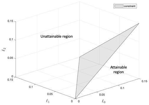
Figure 1 Graph of the geoengineering design space, with the axes representing the ℓ₀, ℓ₁, and ℓ₂ injected per degree of global warming. The triangle represents the approximated constraint of ${\mathrm{\ell }}_{\mathrm{0}}\ge \left|{\mathrm{\ell }}_{\mathrm{1}}\right|+\left|{\mathrm{\ell }}_{\mathrm{2}}\right|$; subject to nonlinearities affecting the constraint, points on or underneath the triangle can be reached by choosing the injection rates at some or all of 30^∘ S, 15^∘ S, 15^∘ N, and 30^∘ N.

We now begin to introduce surfaces to the design space graph to represent different climate objectives. Each surface shows all combinations of AOD achievable with the GLENS injection scheme that will meet that objective; therefore, all surfaces presented here will be placed in the “attainable region” of the ℓ₀–ℓ₁–ℓ₂ space shown in Fig. 1. In this study, we define one climate objective for each of the six chosen metrics, which is to restore that metric to its average value during the years 2010–2030 of the Representative Concentration Pathway (RCP) 8.5 simulations of Tilmes et al. (2018), averaged across all ensemble members. MacMartin et al. (2017) approximated that T₀, T₁, and T₂ respond linearly to small changes in ℓ₀, ℓ₁, or ℓ₂ near their respective reference values; we make the same approximation for our three new metrics. As such, all of the six climate goals can be met with linear combinations of ℓ₀, ℓ₁, and ℓ₂, and therefore each surface considered in this study will manifest as a plane defined by an equation of the form $\mathit{\alpha }{\mathrm{\ell }}_{\mathrm{0}}+\mathit{\beta }{\mathrm{\ell }}_{\mathrm{1}}+\mathit{\gamma }{\mathrm{\ell }}_{\mathrm{2}}=\mathit{\delta }$. The right-hand side, δ, represents the desired change in the climate metric, and α, β, and γ denote the respective sensitivities of the metric to changes in ℓ₀, ℓ₁, or ℓ₂, respectively (i.e., the orientation of the plane). Therefore, each term on the left-hand side of the equation represents the change in the metric caused by 1 degree of freedom, and when those three changes sum to the total desired change, the objective is satisfied.

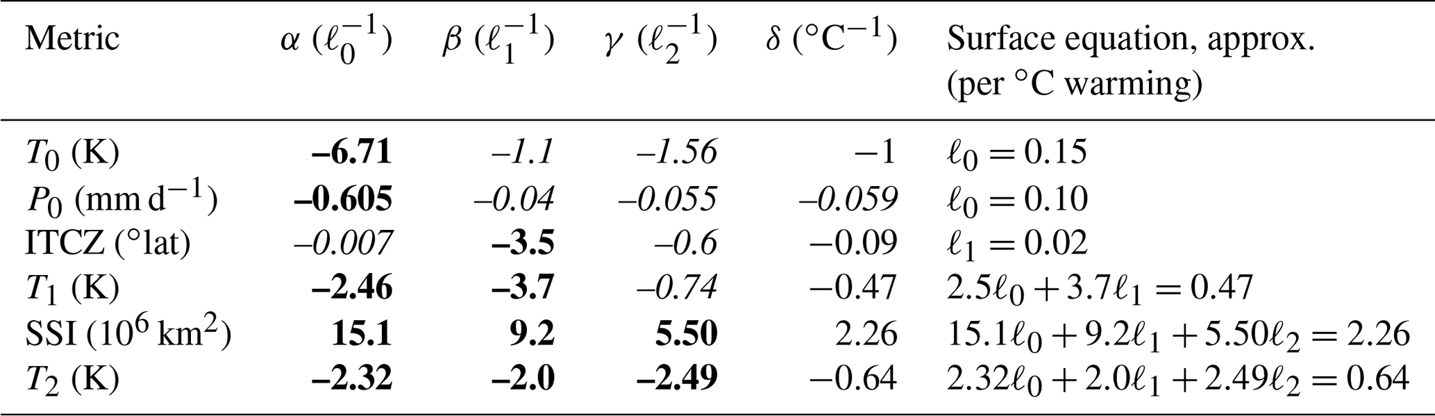
Table 1 Surface equation components for six climate metrics (significant digits are based on standard error). α, β, and γ represent metric responses to changes in ℓ₀, ℓ₁, and ℓ₂, respectively; bolded numbers indicate dominant sensitivities, and those given in italics are approximated as negligible. δ represents the change in each metric per degree of warming required to restore that metric to its 2010–2030 average under RCP8.5. The surface equation is defined by $\mathit{\alpha }{\mathrm{\ell }}_{\mathrm{0}}+\mathit{\beta }{\mathrm{\ell }}_{\mathrm{1}}+\mathit{\gamma }{\mathrm{\ell }}_{\mathrm{2}}=\mathit{\delta }$, with any italicized sensitivities replaced by 0.

To estimate α, β, and γ for each metric, we examine the behavior of each metric in multiple past simulations and fit a linear regression model to the change in that metric (relative to RCP8.5) as a function of the ℓ₀, ℓ₁, and ℓ₂ present in that simulation. We used three different datasets in order to obtain linearly independent combinations of ℓ₀, ℓ₁, and ℓ₂. We use the years 2075–2095 of the GLENS study (Tilmes et al., 2018), the years 2075–2095 of a simulation in which global mean temperature was regulated via equatorial injection (Kravitz et al., 2019), and the years 2044–2049 in six simulations (Tilmes et al., 2017; MacMartin et al., 2017) in which aerosols were injected at constant rates at prescribed latitudes (12 Tg SO₂ yr⁻¹ at each of 15^∘ N, 15^∘ S, 30^∘ N, 30^∘ S; 30^∘ N and 15^∘ N together; and 30 and 15^∘ S together; and 6 Tg SO₂ yr⁻¹ at all four latitudes together). We treat each year of simulation as an independent sample, which yields 519 data points: 420 from GLENS (21 years of simulation multiplied by 20 ensemble members), 63 from the equatorial injection study (21 years of simulation multiplied by 3 ensemble members), and 36 from the prescribed-latitude injection study (6 years of simulation multiplied by 6 simulations). Fitting a linear regression model to the change in each metric relative to RCP8.5 during each year of simulation as a function of the ℓ₀, ℓ₁, and ℓ₂ present in that year yields our estimates for α, β, and γ, which we present in Table 1.

Uncertainty in these estimates arises both through natural variability and due to limitations of the data sources used in this analysis. The equatorial injection study injected at a latitude other than the four used in the GLENS scheme, and the prescribed-latitude injection simulations were only 10 years long; we discard the initial 4 years to avoid the initial transient (see MacMartin et al., 2017), but the climate response will still not yet be in steady state over the remaining 6 years. The prescribed-latitude simulations were also conducted using an earlier version of the land model (CLM4 rather than CLM4.5). We also observe that our sensitivity estimates for temperature-based metrics are different from those of MacMartin et al. (2017). The discrepancies are likely due to the difference in the quantity of data available; the estimates of MacMartin et al. (2017) were based solely on 10-year simulations in which the climate response had not yet converged, and it is therefore likely that they underpredicted the climate response. This is consistent with the signs of the differences in our estimates; our estimates for the dominant sensitivities of T₀, T₁, and T₂ are approximately 20 % larger, 2–3 times larger, and 4–5 times larger than those of MacMartin et al. (2017), respectively. While the differences are not trivial, we present these calculations not to establish the ground truth of how much each metric changes in the presence of aerosols but rather to demonstrate the process of creating our design space visualization and feedback algorithms by showing that certain degrees of freedom in AOD have much greater effects on certain metrics than others. Ultimately, our calculations allow us to draw the same conclusions regarding the relative sizes of sensitivities of climate metrics to AOD as those drawn by MacMartin et al. (2017) (e.g., that T₀ depends primarily on ℓ₀), and as our results will show in Sect. 7, the sensitivities do not need to be perfect estimates as long as they are close enough for the feedback algorithm to converge.

For each metric, δ in Table 1 represents the change in that metric necessary to return that metric from its 2075–2095 RCP8.5 condition to its 2010–2030 reference condition. In order to make the surfaces agnostic to the amount of warming in the background scenario, we normalize δ by the amount of warming in RCP8.5 by the 2075–2095 period, which averages to 4.05 ^∘C. Therefore, by definition, $\mathit{\delta }=-\mathrm{1}$ for T₀, as the goal is to offset exactly 1 ^∘C of T₀ for each 1^∘C of global warming. For other metrics, such as the ITCZ, the δ value of −0.09 indicates that, in order to satisfy the ITCZ objective, the aerosols need to push the ITCZ south by 0.09^∘ latitude for each 1 ^∘C of global warming in the background scenario. The exception to the rule is SSI; while we approximate that SSI responds linearly to small changes in forcing near its reference value, the desired change in SSI is only proportional to the required changes in forcing up until SSI drops to zero around the year 2040. After this point, the desired change in SSI remains constant, but since the background warming continues to increase, the amount of forcing required to restore SSI to its reference condition also continues to increase. Therefore, the difference between the SSI reference value and the 2075–2095 RCP8.5 average SSI of zero does not accurately reflect the forcing required to restore SSI to its reference condition during the 2075–2095 period. To adjust for this, instead of using 0 for the RCP8.5 value of SSI in 2075–2095, we extrapolate from the behavior of sea ice during the linear region of 2020–2040 in GLENS and compute the value SSI would have in 2075–2095 if it were allowed to drop below zero, which is approximately $-\mathrm{6.7}\times {\mathrm{10}}^{\mathrm{6}}$ km². While a negative amount of sea ice is obviously nonphysical, the amount of forcing required to restore sea ice is now proportional to the desired “change”, and as our results will demonstrate, this method permits us to accurately estimate the forcing required to restore SSI to its reference value.

With all four unknowns calculated, we can write the equation for each surface by setting $\mathit{\alpha }{\mathrm{\ell }}_{\mathrm{0}}+\mathit{\beta }{\mathrm{\ell }}_{\mathrm{1}}+\mathit{\gamma }{\mathrm{\ell }}_{\mathrm{2}}=\mathit{\delta }$, as shown in the last column of Table 1. However, as discussed earlier, the feedback algorithms of Kravitz et al. (2017) neglected small sensitivities; for example, MacMartin et al. (2017) estimated the influence of ℓ₀ on T₀ to be an order of magnitude larger than the respective influences of ℓ₁ and ℓ₂, and therefore neglected the latter. This approximation greatly simplified the design process of their feedback algorithm, and as demonstrated by their results, the uncertainty reduction provided by the application of feedback was sufficient to compensate for the errors introduced by the approximation. Therefore, when writing our surface equations in the last column of Table 1, we make the same approximation: since MacMartin et al. (2017) and Kravitz et al. (2017) safely neglected the influences of ℓ₁ and ℓ₂ on T₀, and we compute those sensitivities to be at least 4 times smaller than that of ℓ₀, we neglect any sensitivities which are at least 4 times smaller than the dominant influence. For example, we estimate the influence of ℓ₁ on the ITCZ (β=0.35^∘ per unit ℓ₁) to be 7 times as large as the influence of ℓ₂ (γ=0.05^∘ per unit ℓ₂) and several orders of magnitude larger than the influence of ℓ₀ ($\mathit{\alpha }=-\mathrm{0.002}$^∘ per unit ℓ₀). We indicate this in Table 1 by bolding the dominant sensitivity and italicizing the neglected ones, and when writing the ITCZ surface equation in the last column of Table 1, we approximate that the ITCZ depends only on ℓ₁ and does not respond at all to changes in ℓ₀ or ℓ₂. Similarly, we approximate T₀ as only depending on ℓ₀, T₁ as depending on ℓ₀ and ℓ₁, and T₂ as depending on all 3 degrees of freedom, which are the same approximations made by the GLENS study (MacMartin et al., 2017). We also approximate P₀ as depending only on ℓ₀, and SSI as depending on all three. Like in Kravitz et al. (2017) and MacMartin et al. (2017), these approximations will greatly simplify the design of the feedback algorithms we will present in Sect. 6, and as our results will show in Sect. 7, the inherent uncertainty reduction of feedback is sufficient to compensate for the errors introduced by the approximations. Additionally, simplifying the equations substantially increases the visual clarity of our design space model without changing any of the core results (i.e., whether two surfaces intersect, and where).

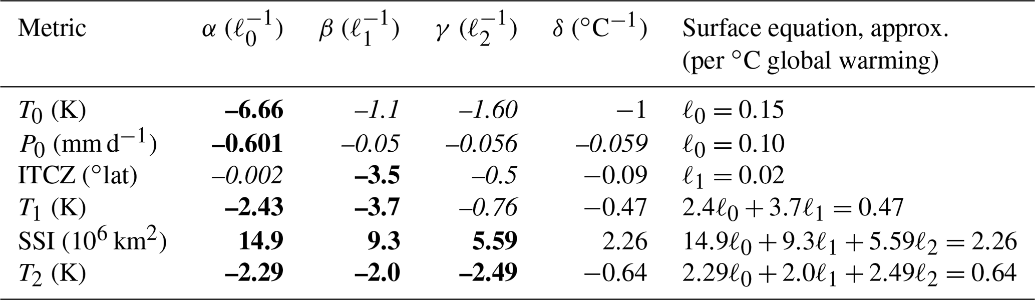
We will now add the surfaces represented by the equations in the last column of Table 1 to the design space graph. In Fig. 2, we add a dark gray surface representing global mean temperature (T₀). As shown in Table 1, T₀ is dominantly dependent on ℓ₀ and largely independent of the other 2 degrees of freedom; as such, we approximate the T₀ surface as a plane normal to the ℓ₀ axis with the equation ℓ₀≈0.15 ^∘C⁻¹ of warming (had we incorporated the estimated dependencies on ℓ₁ and ℓ₂ into the orientation of the surface, the surface would have a slight “tilt” relative to the ℓ₀ plane). Bounding the plane with the AOD constraint produces a triangle, shown in Fig. 2. This triangle represents all of the combinations of AOD in the achievable design space that will control T₀; hypothetically, any point on the triangle – that is, any pattern of AOD with ℓ₀≈0.15 ^∘C⁻¹ of warming – will restore T₀. Any point closer to the origin (ℓ₀<0.15 ^∘C⁻¹) will undercompensate global mean temperature, leaving residual warming, while any point beyond the surface (ℓ₀>0.15 ^∘C⁻¹) will overcompensate global mean temperature, causing excess cooling.

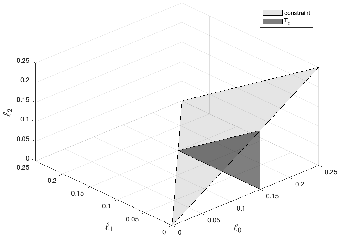
Figure 2 The geoengineering design space. The dark triangle representing T₀, given by the equation ℓ₀≈0.15, represents all achievable combinations of AOD that will return T₀ to its reference condition.

Figure 3 The geoengineering design space (two metrics). We add a second smaller dark triangle to represent AOD combinations that will control P₀; the two dark gray surfaces do not intersect, which indicates that T₀ and P₀ cannot be managed simultaneously.

In Fig. 3, we add a second dark gray surface to represent global mean precipitation (P₀). Like global mean temperature, P₀ depends primarily on ℓ₀, and so we will also model the P₀ surface with a plane parallel to the ℓ₀ axis, placed at ℓ₀=0.10 ^∘C⁻¹ of warming. Because controlling P₀ requires significantly less ℓ₀ than managing T₀ does, the surfaces for T₀ and P₀ do not intersect (this would still be true if the small ℓ₁ and ℓ₂ dependencies were incorporated into both surfaces). This indicates that it is not possible to control both metrics simultaneously, which is consistent with our understanding that global mean temperature and global mean precipitation cannot be managed at the same time using stratospheric sulfate aerosol geoengineering; while a mixed strategy utilizing both aerosol injection and cirrus cloud thinning may be successful at managing both variables (Cao et al., 2017), an approach using only stratospheric sulfate aerosol injection cannot simultaneously restore global mean temperature and global mean precipitation to the same pre-warming levels (Bala et al., 2008; Tilmes et al., 2013; Kravitz et al., 2013).

Figure 4 The geoengineering design space (three metrics). The red triangle represents AOD combinations that will control the ITCZ; unlike T₀ and P₀, which depend primarily on ℓ₀, the ITCZ is primarily influenced by ℓ₁. Intersections between surfaces indicate AOD combinations that can manage multiple metrics simultaneously.

In Fig. 4, we add another surface to the graph: the red triangle represents all possible combinations of AOD that will manage the ITCZ. Unlike the metrics T₀ and P₀, which have dominant dependencies on global mean AOD, the position of the ITCZ is influenced primarily by the hemispheric AOD distribution (Haywood et al., 2013), and so the surface is normal to the ℓ₁ axis instead of the ℓ₀ axis. Placed at ℓ₁≈0.02 ^∘C⁻¹ of warming, the red triangle intersects with both the T₀ and P₀ surfaces; these intersections indicate that it is possible to manage both the ITCZ and either of the ℓ₀-dependent metrics at the same time. The AOD combinations necessary to accomplish this are given by the locations of the intersections on the graph; the T₀ and ITCZ triangles intersect at the vertical line (ℓ₀≈0.15, ℓ₁≈0.02), and so a geoengineering strategy with ℓ₀≈0.15 and ℓ₁≈0.02 (per ^∘C of warming) will successfully control both metrics, regardless of ℓ₂. Likewise, a strategy with ℓ₀≈0.10 and ℓ₁≈0.02 (per ^∘C of warming) will manage both P₀ and the ITCZ simultaneously.

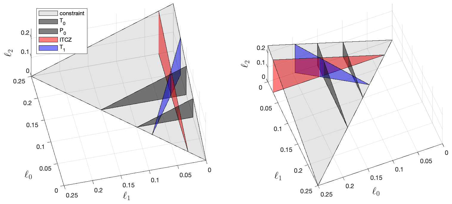
Figure 5 The geoengineering design space (four metrics). The blue triangle represents T₁, which has substantial dependencies on both ℓ₀ and ℓ₀, intersecting all three of the previous surfaces at an angle.

In Fig. 5, we add a blue surface to the graph representing T₁. Like the ITCZ, T₁ responds to changes in ℓ₁, but unlike the ITCZ, T₁ also has a substantial dependence on ℓ₀ which cannot be neglected; this is consistent with the observation that T₁ changes under global warming because the Northern Hemisphere has more land and therefore warms faster than the Southern Hemisphere (Schneider et al., 2014). While the ITCZ is also expected to shift slightly with climate change, the expected shift is relatively small; as such, while the red ITCZ surface can be approximated as normal to the ℓ₁ axis, the blue T₁ surface is not perpendicular to either the ℓ₀ nor the ℓ₁ axis but is diagonal on the ℓ₀–ℓ₁ plane, defined by the equation $\mathrm{2.4}{\mathrm{\ell }}_{\mathrm{0}}+\mathrm{3.7}{\mathrm{\ell }}_{\mathrm{1}}\approx \mathrm{0.47}$ ^∘C⁻¹ of warming. The blue triangle intersects with each of the P₀, T₀, and ITCZ surfaces, indicating that T₁ could be controlled alongside any one of these three metrics. However, since there is no place where three surfaces intersect together, only two of these metrics can be managed at once. For example, consider the intersection of the dark gray T₀ triangle and the blue T₁ triangle at the vertical line ℓ₀≈0.15, ℓ₁≈0.03; the intersection indicates that it is possible to manage T₀ and T₁ concurrently using this combination of AOD. However, this combination requires overcompensating the ITCZ, as an ℓ₁ of 0.03 is more than the 0.02 required to perfectly restore the ITCZ as defined by the red surface. This assertion is validated by the GLENS study, which produced a similar combination of AOD and successfully managed both T₀ and T₁ but overcompensated the ITCZ by about 50 % (see Table 3, Sect. 7; note that Kravitz et al., 2019 and Cheng et al., 2019 compute different results from GLENS because they use the global precipitation centroid, which is a poorer proxy for the ITCZ than the tropical precipitation centroid used here). The ability to visualize such mutually exclusive combinations of climate goals illustrates the power of our model in establishing the fundamental limits and trade-offs of geoengineering, which we will discuss more in Sect. 8.

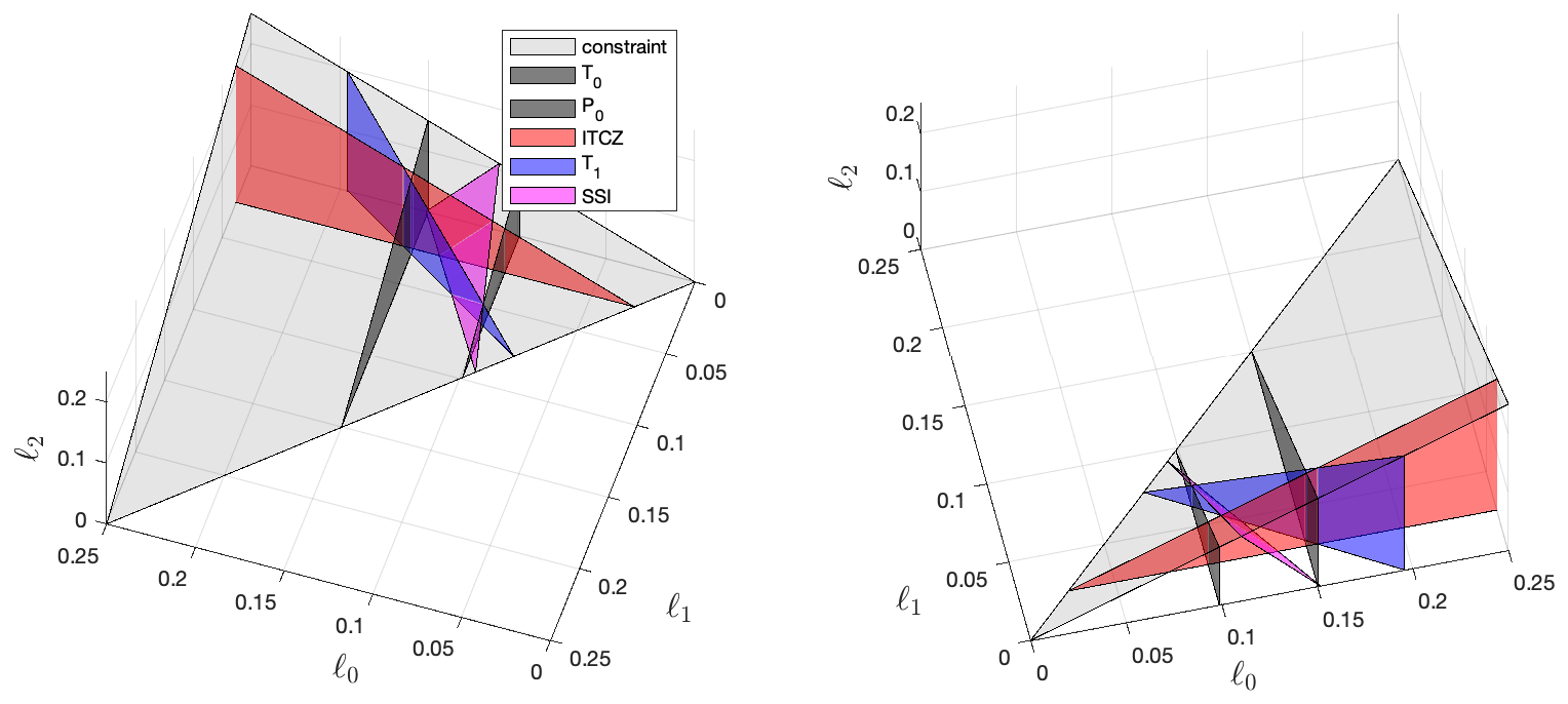
Figure 6 The geoengineering design space (five metrics). The pink triangle, representing SSI, has substantial dependencies on all 3 degrees of freedom. As the first introduced metric to have a substantial ℓ₂ dependence, observe that the pink triangle has a vertical slant.

Figure 6 introduces a pink triangle which represents the combinations of AOD that will manage SSI. All 3 degrees of freedom have significant influences on this climate metric, and therefore the resultant surface, defined by the equation $\mathrm{14.9}{\mathrm{\ell }}_{\mathrm{0}}+\mathrm{9.3}{\mathrm{\ell }}_{\mathrm{1}}+\mathrm{5.6}{\mathrm{\ell }}_{\mathrm{2}}\approx \mathrm{2.26}$ ^∘C⁻¹ of warming, appears slanted rather than perpendicular to any of the axes. The SSI surface intersects with all four of the previous surfaces, indicating that SSI is mutually compatible with any of these climate goals. For example, T₀ and SSI intersect very near to the point (ℓ₀≈0.15, ${\mathrm{\ell }}_{\mathrm{1}}\approx {\mathrm{\ell }}_{\mathrm{2}}\approx \mathrm{0}$0, indicating that while our T₀ and SSI objectives may be achieved together, this is only possible with very low quantities of ℓ₁ and ℓ₂; this is again consistent with the GLENS simulations, which controlled T₀ but overcompensated SSI (Jiang et al., 2019) because they produced non-zero quantities of ℓ₁ and ℓ₂ to manage T₁ and T₂, respectively. Likewise, P₀ and SSI are also mutually compatible, but the intersection of (${\mathrm{\ell }}_{\mathrm{0}}\approx {\mathrm{\ell }}_{\mathrm{1}}\approx \mathrm{0.09}$, ℓ₂≈0) indicates that nearly all of the forcing would have to be weighted towards the Northern Hemisphere. This would likely have severe consequences for tropical precipitation, as the ℓ₁ of 0.09 required to accomplish this is much larger than the 0.02 necessary to return the ITCZ to its reference value.

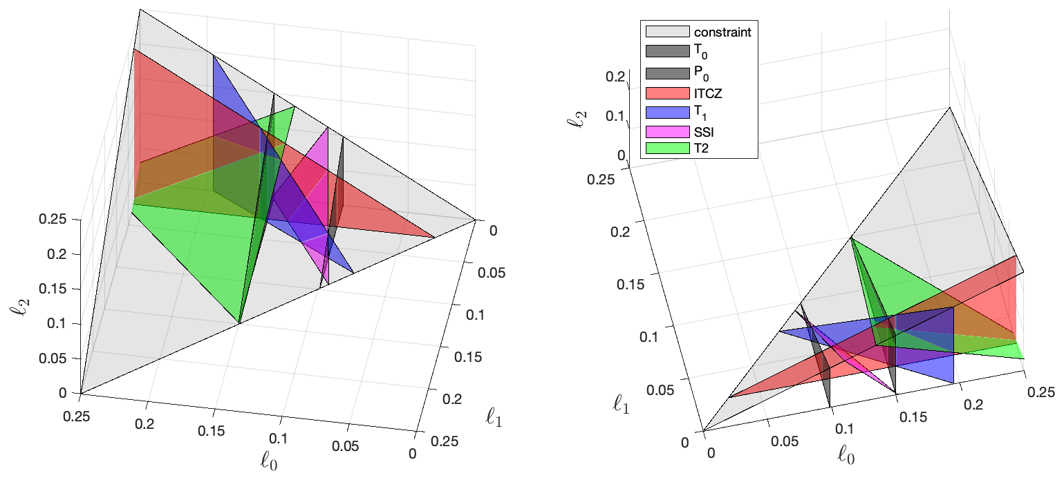
Figure 7 The geoengineering design space (six metrics). The green triangle represents T₂, the last of the six metrics considered in this study. Like the pink SSI surface, the green T₂ surface depends on all 3 degrees of freedom.

In Fig. 7, we complete our design space model by introducing a green triangle to represent T₂, the last of the six metrics we consider in this study. Like SSI, T₂ is sensitive to changes in all three AOD degrees of freedom, and we model the green T₂ surface with the equation $\mathrm{2.3}{\mathrm{\ell }}_{\mathrm{0}}+\mathrm{2}{\mathrm{\ell }}_{\mathrm{1}}+\mathrm{2.5}{\mathrm{\ell }}_{\mathrm{2}}\approx \mathrm{0.64}$ ^∘C⁻¹ of warming. The T₂ surface intersects with each of the T₀, T₁, and ITCZ surfaces, but the placement of the surface further out along the ℓ₀ axis indicates that managing T₂ requires significantly more AOD than P₀ or SSI, making T₂ incompatible with either of the latter options. We observe that the T₀, T₁, and T₂ surfaces all intersect at the point (ℓ₀≈0.15, ℓ₁≈0.03, ℓ₂≈0.10), which indicates that these three climate goals can be met simultaneously; however, the GLENS simulations attempted to accomplish this but could not completely restore T₂, only offsetting about 80 % of the increase caused by global warming. As such, it appears that at this rate of injection, the nonlinear nature of AOD production makes the true constraint more restrictive than our linear approximation of ${\mathrm{\ell }}_{\mathrm{0}}\ge {\mathrm{\ell }}_{\mathrm{1}}+{\mathrm{\ell }}_{\mathrm{2}}$ such that the combination of ℓ₀≈0.15, ℓ₁≈0.03, ℓ₂≈0.10 is actually outside of the attainable region of our design space model. We further discuss the implications of this discrepancy, and ways in which it might be surpassed, in Sects. 7 and 8.

4 Simulation design

With our design space model fully established, we now introduce simulations of two new feedback-regulated aerosol injection strategies. Like the simulations of GLENS and its predecessor Kravitz et al. (2017), each new simulation we present here attempts to simultaneously manage three climate metrics that depend on all 3 degrees of freedom. The purpose of these simulations is two-fold: firstly, we use our design space visualization to choose climate objectives for each of our simulations, and the simulations validate our model by producing results consistent with the model's expectations. Secondly, by including non-temperature-based goals among the climate objectives for each strategy, our simulations demonstrate that we can meet precipitation-based objectives with feedback-regulated SO₂ injection, and that we can manage sea ice alongside other metrics through injections at multiple locations.

Our first simulation attempts to manage T₀, the ITCZ, and SSI simultaneously, and the second attempts to control P₀, the ITCZ, and SSI simultaneously. In each case, the feedback algorithm attempts to restore each climate metric to its reference condition as defined in Sect. 2 (the 2010–2030 average of that metric under RCP8.5). Each of these combinations produces a triangular influence matrix similar to that of Kravitz et al. (2017) and GLENS: T₀ and P₀ depend primarily on ℓ₀, the ITCZ depends primarily on ℓ₁, and SSI is the only metric in each set to depend on ℓ₂. As such, just as in Kravitz et al. (2017), our algorithms will first adjust ℓ₀ based on the behavior of T₀ or P₀, then adjust ℓ₁ based on the behavior of the ITCZ, and then adjust ℓ₂ based on the behavior of SSI. As shown in Fig. 7, our design space model shows that the T₀ and ITCZ surfaces intersect, and that the P₀ and ITCZ surfaces intersect; therefore, in each case, our visualization predicts that our feedback algorithms can choose combinations of ℓ₀ and ℓ₁ that meet their first two objectives. However, the SSI surface does not coincide with either of these intersections, which means that in both simulations, our design space model predicts that the controller cannot choose an ℓ₂ to satisfy the SSI objective given the ℓ₀ and ℓ₁ already chosen to satisfy the other two. Additionally, based on the relative positioning of the surfaces in Fig. 7, our visualization also predicts the behavior of SSI in each simulation. In the case of the first simulation (T₀/ITCZ/SSI), the T₀/ITCZ intersection is located beyond the SSI surface, indicating that the ℓ₀ and ℓ₁ chosen to manage the first two objectives will already produce more than enough forcing to compensate SSI; to minimize the overshoot, our controller will converge to an ℓ₂ of zero, but the simulation will still overcompensate SSI, resulting in more sea ice than the quantity designated by the objective. In the case of the second simulation (P₀/ITCZ/SSI), the SSI surface is located beyond the P₀/ITCZ intersection, indicating that there is no achievable quantity of ℓ₂ sufficient to return SSI to the desired value given the ℓ₀ and ℓ₁ chosen to manage the first two objectives. In order to restore as much sea ice as possible, the feedback algorithm will converge to the maximum ℓ₂ permitted by the controller constraint, approximated by ${\mathrm{\ell }}_{\mathrm{2}}={\mathrm{\ell }}_{\mathrm{0}}-{\mathrm{\ell }}_{\mathrm{1}}$; however, the simulation will still undercompensate SSI, resulting in less sea ice than the target value.

Rather than simulate the entire 21st century, as in Kravitz et al. (2017) and Tilmes et al. (2018), both of our simulations begin in 2060 by branching from one of the GLENS runs as in Visioni et al. (2020b), and then run until 2095. Like these studies, we also use RCP8.5 as the background warming scenario; while the extremely high emissions in this scenario result in a large amount of warming, the magnitude of warming gives a strong signal-to-noise ratio, especially at the end of the century, and an emulator could project what the results would be for other warming scenarios (MacMartin et al., 2019). Branching in this way allows us to begin our study late in the century, make use of the high signal-to-noise ratio, and compare our results to those of the GLENS study without using unnecessary computer time to simulate the beginning of the century.

5 Climate model

In this study, we use the Community Earth System Model version 1 with the Whole Atmosphere Community Climate Model (Mills et al., 2017) as the atmospheric component, or CESM1(WACCM). The model includes POP2 (ocean), CLM4.5 (land), and CICE4 (ice). The model is run at a horizontal resolution of 0.9^∘ latitude by 1.25^∘ longitude, and WACCM has a vertical grid of 70 layers up to an altitude of 145 km (approximately 10⁻⁶ hPa). As in Tilmes et al. (2018), SO₂ is injected at 30^∘ S, 15^∘ S, 15^∘ N, and 30^∘ N, approximately 5 km above the annual-mean tropopause (thus at 25 km for 15^∘ N/S and 23 km for 30^∘ N/S). The aerosol component, MAM3 (Liu et al., 2012), uses a trimodal distribution and is fully coupled to both atmospheric chemistry and radiation. The model has been validated against observations after volcanic eruptions (Mills et al., 2016, 2017, using CLM4); the version used here includes the updated land model version CLM4.5 as described in Tilmes et al. (2018). As in Kravitz et al. (2017), injection rates at each latitude are governed by a feedback algorithm which adjusts injection rates annually based on the deviation of the metrics from their desired values (see Sect. 6 for a more detailed description of the feedback algorithms used in this study).

6 Feedback algorithm design

Each of the two simulations in this study incorporates a control algorithm which determines how much aerosol to inject during each year of simulation in order to simultaneously manage three chosen climate metrics. The algorithm applies both feedforward and feedback; the feedforward consists of estimates made before the simulation of how much AOD will be needed as a function of time, and the feedback makes small corrections during the simulation based on the actual behavior of the metrics to account for imperfections in the feedforward. Once the feedforward and feedback determine the appropriate combination of ℓ₀, ℓ₁, and ℓ₂, the algorithm then computes how much SO₂ to inject at each of 30^∘ N, 15^∘ N, 15^∘ S, and 30^∘ S in order to produce that combination using the transformations given by Eq. (5). This section assumes basic familiarity with feedback control theory; for a more detailed introduction to geoengineering feedback algorithms, we recommend MacMartin et al. (2017), Kravitz et al. (2017, 2016), and MacMartin et al. (2014), who developed the original algorithms upon which ours are based. For a more general introduction to feedback control, we recommend Feedback Systems: An Introduction for Scientists and Engineers by Aström and Murray (2008).

The feedforward gains for each simulation prescribe the amounts of ℓ₀, ℓ₁, and ℓ₂ to be produced each year based on the expected AOD needed to manage the three target metrics. As discussed in Sect. 2, each climate metric considered here responds roughly proportionally to small changes in forcing in the area of ℓ₀–ℓ₁–ℓ₂ space in which we operate. Since global warming under RCP8.5 increases proportionally, or nearly proportionally, with time, the AOD required to counteract those changes will also increase linearly with time. Thus, while in general, the feedforward might be a more complicated function of time (e.g., Tilmes et al., 2020), in this study, the feedforward can be expressed more simply as three constant gains prescribing the estimated increases in ℓ₀, ℓ₁, and ℓ₂ per year necessary to meet the given climate goals. For each simulation, we compute these feedforward gains by first estimating the average values of ℓ₀, ℓ₁, and ℓ₂ necessary to control the three metrics in the years 2075–2095 according to our design space model. While the estimates based on our model alone would likely be sufficient to meet our chosen climate goals alongside the use of feedback, we attempt to further increase the accuracy of the feedforward by compensating for some of the nonlinearities in the production of AOD in order to reduce the burden on the feedback. We do this by relating the AOD requested by the GLENS controller to the actual AOD produced by the GLENS simulations. Once we know how much total AOD the controller should request (on average) in the year 2085, we know that we want the controller to increase linearly towards that amount from zero AOD beginning in 2020, so we divide the 2085 AOD by 65 years to finalize the feedforward gains. These values are presented below. Note that the gains provided here were based on previous iterations of the design space graph and do not reflect our current best estimates; more information about their derivation is provided in Appendix B.

The feedback gains for each simulation prescribe adjustments to the ℓ₀, ℓ₁, and ℓ₂ to be injected each year based on the deviation of each metric from its desired state. The algorithms used in this study use proportional–integral feedback, meaning two distinct corrections are applied: one proportional to the magnitude of the error and one proportional to the integral of the error over time. As in Kravitz et al. (2017), the integral feedback gains for ℓ₀, ℓ₁, and ℓ₂ each will equal their respective proportional feedback gains (Kravitz et al., 2016). We wish to achieve the same 5-year convergence time as in Kravitz et al. (2016, 2017); therefore, we use the same feedback gains scaled by the ratio of the appropriate metric sensitivities, which will recover the same behavior. These feedback gains are also presented below. As with the feedforward estimates, those provided here are based on prior sensitivity estimates and do not reflect our current best estimates for the optimal feedback gains to produce the desired convergence time; more information is available in Appendix B.

Table 2 Equations for the ℓ₀, ℓ₁, and ℓ₂ to be injected in each year of our simulations. The first term in each equation represents the feedforward; the second and third terms represent the proportional and integral feedbacks, respectively. Any additional terms represent corrections based on the appropriate metric's sensitivities to the 3 degrees of freedom. Only the feedforwards are used during the first 5 years of simulation; after the first 5 years, the entire equations are applied.

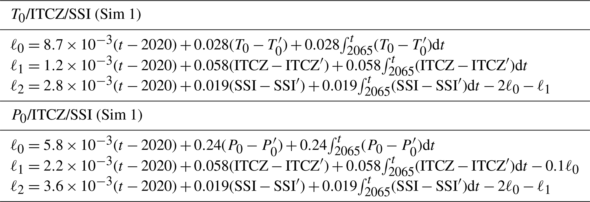
For the first 5 years of simulation, only the feedforward is used; beginning in 2065, the feedforward and feedback corrections are then summed in order to determine how much ℓ₀, ℓ₁, and ℓ₂ to inject during the following year, as shown in Table 2; the first term in each equation represents the feedforward, and the second and third terms represent the proportional and integral feedbacks, respectively. Additionally, since ℓ₀ and ℓ₁ affect SSI, we account for those changes by subtracting factors of the computed ℓ₀ and ℓ₁ based on the relative sensitivities of SSI to each degree of freedom (we do the same for the ITCZ in our second simulation; see the Appendix for more details). As discussed previously, combinations of AOD with ${\mathrm{\ell }}_{\mathrm{0}}\ge \left|{\mathrm{\ell }}_{\mathrm{1}}\right|+\left|{\mathrm{\ell }}_{\mathrm{2}}\right|$ are not attainable using the four-latitude injection scheme. Therefore, the controller must prioritize its objectives in the event that it cannot produce the AOD required to meet all of them. The order in which the feedback algorithm prioritizes objectives is a design choice; in this study, we use the same prioritization scheme as in Kravitz et al. (2017), which prioritizes the ℓ₀ objective first, the ℓ₁ objective second, and the ℓ₂ objective last. Therefore, if the requested values of ℓ₀, ℓ₁, and ℓ₂ violate the inequality ${\mathrm{\ell }}_{\mathrm{0}}\ge \left|{\mathrm{\ell }}_{\mathrm{1}}\right|+\left|{\mathrm{\ell }}_{\mathrm{2}}\right|$, the controller will satisfy the inequality by first reducing ℓ₂ and then (if ℓ₂ cannot be reduced further and the constraint is still violated) by reducing ℓ₁. Once the inequality has been satisfied, the algorithm converts the finalized values of ℓ₀, ℓ₁, and ℓ₂ into the quantities of SO₂ to be injected at 30^∘ S, 15^∘ S, 15^∘ N, and 30^∘ N during the next year of simulation. This conversion is accomplished by solving the linear system described in Eq. (5), which relates injections at the chosen latitudes to the production of ℓ₀, ℓ₁, and ℓ₂. As discussed earlier, while the conversions from requested AOD to injection rates to actual AOD are modeled as linear within the controller, the actual process is nonlinear. As a result of this, the actual AOD produced will always be different from the AOD commanded by the controller, and the difference worsens at higher injection rates (Visioni et al., 2020a). However, because the application of feedback manages uncertainty, there is a substantial amount of tolerance built into the algorithm, and our results demonstrate that our controller converges despite the nonlinearities present in the production of AOD.

7 Results

In Fig. 8, we present the behaviors of the six climate metrics (T₀, T₁, T₂, P₀, ITCZ, and SSI) in our two simulations, as well as in the GLENS simulations and the RCP8.5 simulations for comparison. The dotted black lines indicate the reference value for each metric, equivalent to the 2010–2030 average of the RCP8.5 simulations, which is the target value for simulations in which that metric was controlled. ITCZ and SSI are smoothed with a 5-year running average in all simulations, including individual ensemble members. In Table 3, we present the difference between the 2075–2095 average and the reference value for each metric, as well as the percent restoration and standard error for each metric; we define the percent restoration as the difference between the 2075–2095 average and the RCP8.5 2075–2095 average, normalized by the difference between the reference value and the RCP8.5 2075–2095 average, as given by Eq. (6):

$$\begin{array}{}\text{(6)}& \begin{array}{rl}\mathit{\%}\mathrm{restoration}& ={\displaystyle \frac{\text{actual change}}{\text{change required to restore metric}}}\\ & ={\displaystyle \frac{\text{actual}-\text{RCP}}{\text{reference}-\text{RCP}}}.\end{array}\end{array}$$

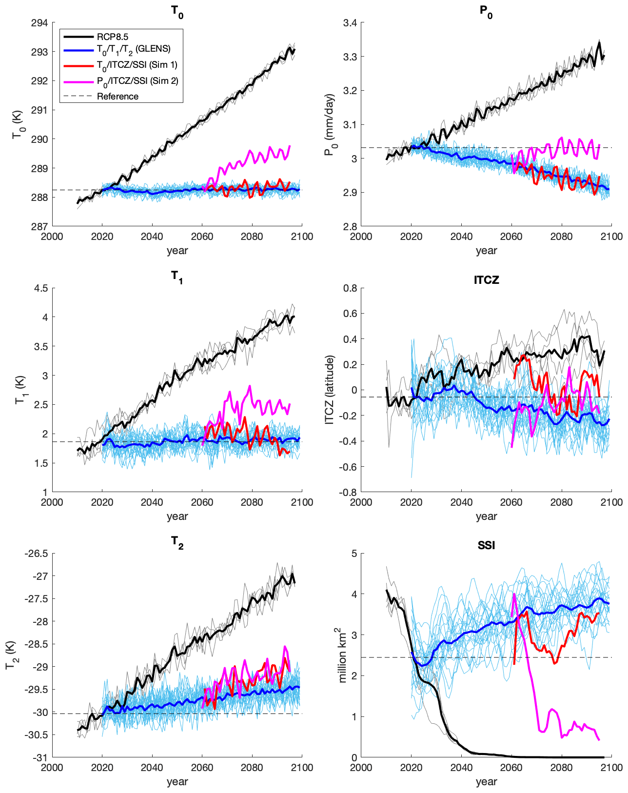
Figure 8 Climate metric behavior over time for our simulations, GLENS, and RCP8.5. ITCZ and SSI are smoothed using a 5-year running average. Thick lines indicate ensemble averages, while faint lines indicate individual ensemble members. Dotted black lines indicate reference values.

Table 3 Differences between simulations (2075–2095 average) and reference value (2010–2030 average), and percent restoration for each metric. Metrics controlled in each simulation are bolded. The asterisk denotes that, as discussed in Sect. 2, we use a negative value for RCP8.5 SSI so that the “change” in SSI is proportional to the change in forcing.

For simulations in which a climate metric was controlled, a restoration value of 100 % is the goal, which indicates that the metric was perfectly restored to its reference value and that geoengineering offset 100 % of the global-warming-induced change in that metric. A restoration value of less than 100 % indicates that a geoengineering strategy did not fully return that climate metric to its reference value, while a restoration value greater than 100 % indicates that a geoengineering strategy overcorrected that particular climate metric, bringing it beyond its reference value. In evaluating the effectiveness of each strategy, we look only at the individual restoration values for each metric; we have made the conscious decision to not attempt to create an overall “restoration score” for each simulation by averaging or otherwise combining the restoration values, or to otherwise grade how “well” each strategy performed as a whole. To claim one strategy performed “better” or “worse” than another would require weighting different climate goals based on their relative importance. That type of judgment is inherently subjective, and such considerations are beyond the scope of this study.

Table 4 The 2075–2095 averages for AOD produced in each simulation (error is less than 1 % where not listed). We also include estimates of the design space models in Sect. 3 for the AOD to which each simulation will converge given the climate objectives for that simulation and the boundaries of the design space.

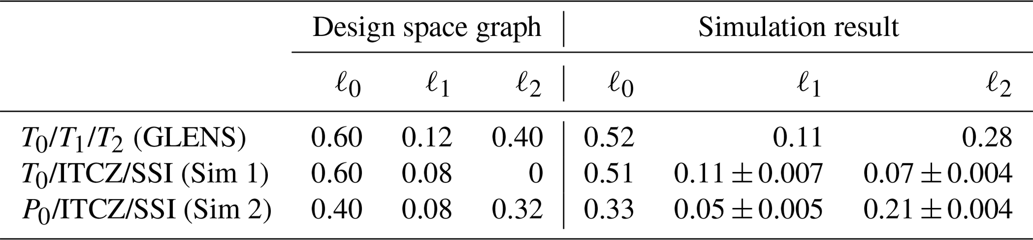
Our first simulation, which controlled for T₀, the ITCZ, and SSI, achieved restoration values of 97 %, 99 %, and 108 %, respectively. The error in managing the ITCZ is well within the limits due to natural variability, and is statistically distinct from the ITCZ behavior in either GLENS or RCP8.5, indicating that actively controlling for ITCZ position by adjusting ℓ₁ achieves the desired outcome. The amount of sea ice restored by the simulation is greater than the desired value, which is consistent with the expectations of our design space model. As expected, managing T₀ and the ITCZ simultaneously requires overcompensating global mean precipitation (148 %) and undercompensating T₂ (68 %); according to the equations in Table 1, for the AOD produced in this simulation (see Table 4 below), the design space graph predicts restoration values of 128 % and 61 %, respectively. We also observe that although our design space graph predicts a T₁ restoration of 87 % for the produced AOD, the simulation restored 98 % of T₁, even though we were not controlling for it. Our second simulation, which controlled for P₀, managed P₀ to within 1 % of its target value, confirming that global mean precipitation can be managed successfully through feedback in a geoengineering simulation. The P₀/ITCZ/SSI simulation also controlled the ITCZ to within 5 % of its target value, which is again statistically significantly different from GLENS and from RCP8.5. As predicted, the simulation significantly undercompensated SSI (81 %). Finally, as predicted by our design space model, the second simulation undercompensated T₀ (71 %, compared to the design space graph's estimate of 67 %), T₁ (68 % vs. 52 %), and T₂ (65 % vs. 54 %). The discrepancies between the expected and actual restoration values for each simulation reflect the approximations described previously in the study (such as the assumption of linear responses to changes in forcing and the neglecting of small sensitivities to certain degrees of freedom), as well as some amount of natural variability; however, we note that in every case, our design space model correctly identifies whether a variable will be overcompensated or undercompensated when a given set of objectives is met.

In Table 4, we present the 2075–2095 averages of ℓ₀, ℓ₁, and ℓ₂ in each of our simulations, as well as the GLENS simulations for comparison; we also present our design space graph's estimates for the quantities of AOD necessary for each simulation to meet its respective climate goals (or, in the case of ℓ₂, the quantity to which the controller will converge as defined by the boundaries of the achievable region of the design space). In each case, the design space graph overpredicts the ℓ₀ necessary to manage the ℓ₀-based metric by 10 %–20 %. In the case of T₀, this is likely due to the influence of ℓ₁ and ℓ₂; while the sensitivities of T₀ to these degrees of freedom are small compared to the effect of ℓ₀, as documented in Table 1, the ℓ₁ and ℓ₂ produced in the GLENS and T₀/ITCZ/SSI simulations decrease the ℓ₀ necessary to manage T₀ by a small amount. In the case of P₀, the sensitivities to the other degrees of freedom are much smaller, and the overprediction is likely due to the fact that, unlike T₀, P₀ has never been controlled in a prior simulation. As the sensitivity data used to develop the design space model are derived from GLENS, which controlled T₀ successfully, it follows that the design space model's expectations for the forcing required to restore T₀ would match the GLENS results; on the other hand, GLENS overcompensated P₀ by about 40 %, and therefore the amount of forcing required to restore P₀ is estimated using the approximation of linearity. As shown by the discrepancies between actual and estimated restoration values earlier in this section, that approximation is largely imperfect, which accounts for the difference between the prediction of our design space model and the actual AOD required in the P₀/ITCZ/SSI simulation. Regardless, the application of feedback to manage uncertainty was sufficient to overcome the discrepancy in both cases, illustrating that prior estimates do not need to be perfect as long as they are close enough for the controller to converge.

Since both new simulations controlled for the ITCZ, the ℓ₁ predicted by the design space graph is the same for both simulations (0.02 per degree of warming, or 0.08). The first simulation (T₀/ITCZ/SSI) converged to a value of 0.11, while the second (P₀/ITCZ/SSI) converged to 0.05; given the large natural variability of the ITCZ and the spacing of the results of the two simulations on either side of the original estimate, it is likely that our estimate of 0.08 is largely correct and that the difference is due to natural variability. It is also possible that the different quantities of ℓ₂ produced in each simulation had a small effect; according to Table 1, ℓ₂ does have a small impact on the ITCZ, and the first simulation (which needed more ℓ₁) had much less ℓ₂ than the second.

The case of ℓ₂ is unique because in none of the three simulations considered here (GLENS and our two new simulations) was the controller able to produce the quantity of ℓ₂ required to meet that simulation's ℓ₂-based objective. In the case of P₀/ITCZ/SSI (our second simulation), the quantity of ℓ₂ required to meet SSI was too high and thus prohibited by the controller constraint, as indicated by the lack of an intersection between P₀, ITCZ, and SSI in Fig. 7; therefore, the predicted ℓ₂ is the largest allowed for that simulation's combination of ℓ₀ and ℓ₁, given by ${\mathrm{\ell }}_{\mathrm{2}}={\mathrm{\ell }}_{\mathrm{0}}-{\mathrm{\ell }}_{\mathrm{1}}$. In the case of GLENS, the combination of AOD required to meet all three objectives does correspond to a three-way intersection in our design space model, but as discussed in Sect. 3, the nonlinear nature of AOD production pushes that point outside of the achievable region in AOD space, and the controller again ends up requesting ${\mathrm{\ell }}_{\mathrm{2}}={\mathrm{\ell }}_{\mathrm{0}}-{\mathrm{\ell }}_{\mathrm{1}}$. In the case of T₀/ITCZ/SSI, the combination of ℓ₀ and ℓ₁ requested by the controller to meet the T₀ and ITCZ climate objectives is already too much to meet the SSI objective; therefore, our controller converged to zero ℓ₂ by around 2085 in order to produce the smallest increase in sea ice possible. The residual ℓ₂ present in the final years of simulation is due to remaining aerosols from previous years of injection, small quantities produced by the subsequent injections at 15^∘ S, 15^∘ N, and 30^∘ N, or a combination of both.

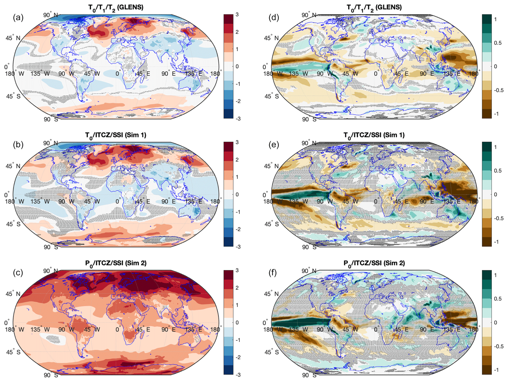
Figure 9 Simulation temperature (a–c) and precipitation (d–f) 2075–2095 averages, relative to the control period (2010–2030 average), for GLENS and our simulations. Gray shading indicates areas where changes are not statistically significant (α=0.05).

In Fig. 9, we present maps of changes in temperature and precipitation for our simulations, as well as those of GLENS for comparison. The changes shown in the figure are the averages over the period of 2075–2095 minus the averages over the 2010–2030 period in the RCP8.5 simulations. Gray shading indicates regions where there is no statistically significant change (α=0.05) between the reference period and the simulation results. The temperature profiles of T₀/T₁/T₂ (GLENS) and T₀/ITCZ/SSI are broadly similar, with most of the globe remaining within 1 ^∘C of the reference period. However, despite controlling for a high-latitude metric, both simulations still demonstrate a small degree of residual polar amplification, in which a geoengineering strategy overcools the tropics and undercools the poles. The temperature profile of T₀/ITCZ/SSI shows more amplification than that of T₀/T₁/T₂ (GLENS), which is consistent with the higher quantities of ℓ₂ produced in the latter (see Table 4 above). Additionally, significantly more of the GLENS profile is statistically distinct from the reference period, but this is more likely the result of the large number of GLENS ensemble members rather than the climate goals chosen or AOD produced. Conversely, the temperatures of P₀/ITCZ/SSI are almost universally warmer than the reference period, an observation consistent with both our design space model's predictions and the understanding that controlling precipitation requires undercompensating for changes in temperature. Changes in precipitation are much more subtle between simulations than changes in temperature; this is likely due to the fact that precipitation is concentrated in the tropics, and so much of the globe has small changes in precipitation regardless of what geoengineering strategy is used. However, there are some consistencies between simulations. All three geoengineering strategies (T₀/T₁/T₂, T₀/ITCZ/SSI, and P₀/ITCZ/SSI) produce similar precipitation anomalies (relative to RCP8.5) over the tropical Pacific, consisting of a drop in precipitation near Malaysia and an increase between the International Dateline and Peru. Again, when compared to the T₀/T₁/T₂ simulations, the precipitation in both of our new simulations shows more statistical similarity to that of the reference period over much of the globe, but again, this is primarily due to the large ensemble size of the former. Figure 10 shows the precipitation changes over India and the Amazon. We observe that the T₀/T₁/T₂ strategy reduces precipitation over Northern India (as observed in Cheng et al., 2019; Simpson et al., 2019; Visioni et al., 2020b), while there is an increase in precipitation in both of our simulations. The T₀/T₁/T₂ strategy also decreases precipitation over the Amazon rainforest, and this reduction intensifies in both of our new simulations.

Figure 10 Precipitation changes over India and the Amazon for GLENS and our simulations, relative to control. Black speckling indicates areas where changes are not statistically significant (α=0.05).

8 Discussion and conclusions

In this study, we produce two new simulations of different SO₂-injection strategies which expand the space of climate objectives considered in geoengineering. While Kravitz et al. (2016) showed that precipitation-based metrics can be controlled in a climate model by using solar reduction as a proxy for aerosol geoengineering, up until now, simulations of stratospheric aerosol injection controlled temperature gradients as proxies for non-temperature-based metrics, such as using T₁ as a proxy for the ITCZ and T₂ as a proxy for sea ice. In addition to demonstrating that three specific climate goals (i.e., control of global mean precipitation, tropical precipitation centroid, and September sea ice in the Arctic Ocean) can be met by adjusting the injection rates independently at four different latitudes, our results demonstrate that feedback algorithms can successfully manage non-temperature-based metrics directly instead of requiring temperature-based proxies, even in the presence of large natural variability, such as with the ITCZ.

In addition to presenting simulations of new strategies for stratospheric aerosol geoengineering, we also present a model for visualizing the geoengineering design space. Our simulations demonstrate the utility of our visualization in assessing the mutual achievability of multiple climate goals, and in assessing how other climate metrics will behave when certain goals are met. Our visualization enabled us to make two specific predictions about the degrees to which certain climate goals could or could not be accomplished together in CESM1(WACCM), and our simulations validated those predictions; additionally, our visualization correctly identified whether meeting those goals would result in the over- or undercorrection of other climate metrics (and, to a lesser extent, the degree of over- or undercorrection).

The general framework could be extended to consider a broader suite of design degrees of freedom; however, the design space model presented here is intended to capture the influence of 3 degrees of freedom via aerosol injection at four specific latitudes. We represent the AOD distribution solely by its projection onto the first three Legendre polynomials; while this approximation was clearly sound enough for the purposes of these simulations, any distribution of AOD will of course contain some projection onto higher-order Legendre polynomials. Changing the injection latitudes in CESM1(WACCM), or evaluating the response in a different climate model, will result in different amounts of those higher-order components. As such, while the sensitivities and surface equations presented in Sect. 3 will likely be valid for any CESM1(WACCM) simulation in which aerosols are injected at only 30^∘ S, 15^∘ S, 15^∘ N, and/or 30^∘ N, more research is needed to validate and improve our sensitivity estimates for simulations in which a different injection scheme or a different climate model is used.

In this study, we only considered one climate objective for each metric (namely, that metric's 2010–2030 average under RCP8.5); however, each metric represents an infinite number of possible climate goals, and each goal could be represented as a surface in our design space model. While we only quantified the surfaces corresponding to each metric's RCP8.5 2010–2030 average, and thus only evaluated intersections where those objectives can be simultaneously reached, our graph provides additional utility in visualizing how the changes in AOD necessary to induce a change in one metric will affect another. For example, our model shows that the overlap between P₀ and SSI is very small, but this does not mean it is impossible to achieve all sets of climate objectives containing one goal based on global mean precipitation and another goal based on sea ice, just that one specific pair of goals is difficult to attain. However, our visualization does indicate that P₀ and SSI both have large dependencies on ℓ₀, and therefore any geoengineering strategy intended to influence global mean precipitation will also have a substantial impact on sea ice, and vice versa. This limits the sets of achievable climate objectives which attempt to control both of these metrics in some way; once the target for P₀ is set, there is a constraint placed on achievable targets for SSI. Conversely, T₀ and the ITCZ depend primarily on different degrees of freedom, which means the two metrics are largely independent. As such, the number of achievable climate states in which T₀ and the ITCZ are both objectives is much larger, as a goal for T₀ places a much smaller constraint (if any) on the ITCZ. In other words, the more parallel two surfaces appear in our visualization, the greater the co-dependency of the metrics; the more perpendicular two surfaces appear, the easier it is to influence those metrics independently and therefore to choose independent goals for those metrics.

In conclusion, we identify several areas of research in which further progress will allow us to continue to develop our design space model by increasing its accuracy, range, and scope of application. Of the three simulations considered in this study, none of them were able to meet all three of their climate objectives simultaneously; however, expanding the design space might make all three sets achievable in future experiments. Firstly, the controller constraint prevents the SSI surface from extending upwards and meeting the intersection of the P₀ and ITCZ surfaces. As discussed previously, meeting all three objectives requires a quantity of ℓ₂ not permitted by the required quantities of ℓ₀ and ℓ₁; identifying the circumstances under which we could move beyond the current constraint, perhaps by injecting at higher latitudes to produce a higher ratio of ℓ₂ to ℓ₀, might make this possible, which would expand the design space and therefore the range of achievable climate goals. The same is true for the combination of T₀, T₁, and T₂. Secondly, expanding the design space in the opposite direction is also possible, as the results of MacMartin et al. (2017) demonstrate that injecting at the Equator can produce a negative ℓ₂, which may permit the SSI surface to extend downward and intersect with the T₀ and ITCZ surfaces. Thus, adding a fifth latitude (i.e., the Equator) to our four-latitude injection scheme could open up a new region of the design space in which the three goals of our first simulation (T₀, ITCZ, and SSI) are simultaneously achievable.

In addition to expanding the design space, taking further steps to quantify our model would improve its accuracy and utility. For example, the T₀–T₁–T₂ intersection appears achievable in our design space model, but we know it not to be based on the results of the GLENS simulations. This is due to the fact that we modeled the controller constraint with a linear approximation, and this approximation holds significantly better at low injection rates than at higher ones. The results presented in Table 3 help quantify the nonlinear relationship between injections and produced AOD, but a more thorough investigation would produce a better model of the controller constraint and thus better clarify which combinations of climate goals are or are not achievable at higher injection rates. Next, beyond the higher-order modes of AOD variability with latitude discussed previously, there are many more degrees of freedom which our model does not even begin to consider, including variations in altitude (e.g., Tilmes et al., 2018), longitude, and season (Visioni et al., 2020a) of deployment. While a higher-dimensional graph would undoubtedly be more difficult for the human mind to visualize, introducing additional degrees of freedom to the model would undoubtedly reveal metric behavior that a 3-D graph cannot account for. Finally, there are far more reasonable choices for climate metrics than the ones considered here, and an infinite number of potential climate objectives; in this study, we consider only six of each. Regardless of the specific objectives chosen for a geoengineering scenario, a thorough understanding of the effects of a given injection strategy on all of these metrics would go a long way towards answering the question of what geoengineering can and cannot accomplish.

Appendix A: Updated sensitivity calculations

In Table A1, we present sensitivity calculations for each of our six climate metrics computed using the two new simulations we presented in this study in addition to the three sources of data described in Sect. 3. We observe that none of the sensitivity variables have changes larger than their last decimal place; no single-variable surface equation has changed, and only the three multi-variable surface equations have small changes to their coefficients. This indicates that in our simulations, climate metrics respond to changes in AOD in a manner largely consistent with the other sources of data, and we include this table only for the sake of completeness.

Table A1 Surface equation components for six climate metrics as in Table 1 but updated using the results of the two new simulations presented in this study. As in Table 1, bolded numbers indicate dominant sensitivities, while those in italics denote those approximated as negligible.

Appendix B: Feedback algorithm calculations

The feedforward gains used in our first simulation were derived from an earlier iteration of the design space model, which based sensitivities and surface placements off of ensemble averages for AOD and metric restoration values from simulation results rather than the least-squares method presented in Sect. 3. This prior method estimated the 2085 AOD necessary to control T₀, the ITCZ, and SSI as ℓ₀=0.52, ℓ₁=0.05, and ℓ₂=0.17. In order to improve the accuracy of the feedforward and reduce the burden on the feedback, we attempted to account for the nonlinearities in AOD production by relating the AOD requested by the controller to the AOD produced for each of ℓ₀, ℓ₁, and ℓ₂; we did this by fitting cubics, provided in Eqs. (B1)–(B3) below, to the relationships between the AOD requested in the GLENS controller logs (denoted with hats) and the AOD produced in each year of the GLENS simulations.

$$\begin{array}{}\text{(B1)}& {\displaystyle }{\mathrm{\ell }}_{\mathrm{0}}=\mathrm{0.5433}{\widehat{\mathrm{\ell }}}_{\mathrm{0}}^{\mathrm{3}}-\mathrm{0.7987}{\widehat{\mathrm{\ell }}}_{\mathrm{0}}^{\mathrm{2}}+\mathrm{1.1930}{\widehat{\mathrm{\ell }}}_{\mathrm{0}}\text{(B2)}& {\displaystyle }{\mathrm{\ell }}_{\mathrm{1}}=-\mathrm{2.4221}{\widehat{\mathrm{\ell }}}_{\mathrm{1}}^{\mathrm{3}}-\mathrm{0.0091}{\widehat{\mathrm{\ell }}}_{\mathrm{1}}^{\mathrm{2}}+\mathrm{0.6978}{\widehat{\mathrm{\ell }}}_{\mathrm{1}}\text{(B3)}& {\displaystyle }{\mathrm{\ell }}_{\mathrm{2}}=\mathrm{0.1688}{\widehat{\mathrm{\ell }}}_{\mathrm{2}}^{\mathrm{3}}-\mathrm{1.5122}{\widehat{\mathrm{\ell }}}_{\mathrm{2}}^{\mathrm{2}}+\mathrm{1.1752}{\widehat{\mathrm{\ell }}}_{\mathrm{2}}\end{array}$$

Substituting the desired values of ℓ₀, ℓ₁, and ℓ₂ into the above equations and solving for ${\widehat{\mathrm{\ell }}}_{\mathrm{0}}$, ${\widehat{\mathrm{\ell }}}_{\mathrm{1}}$, and ${\widehat{\mathrm{\ell }}}_{\mathrm{2}}$ produces ${\widehat{\mathrm{\ell }}}_{\mathrm{0}}$ = 0.5637, ${\widehat{\mathrm{\ell }}}_{\mathrm{1}}$ = 0.0856, and ${\widehat{\mathrm{\ell }}}_{\mathrm{2}}$ = 0.1805. Since we wish to achieve these values in 2085 by linearly increasing from 0 beginning in 2020, we divide each by 65 years to produce the feedforward gains used in Table 2. For the second simulation, we observed that our desired ℓ₀ and ℓ₁ values were approximately two-thirds of those produced in GLENS. Additionally, the maximum ℓ₂ value permitted by this combination would therefore be equal to two-thirds of the value used in GLENS. Therefore, for this simulation, we set our feedforward gains to equal to two-thirds of the AOD produced by GLENS (we did not attempt to account for the nonlinearities present in AOD production as we did in the first simulation).

The feedback gains used for each metric were based on the following prior sensitivity estimates, in which the whole centuries of simulation from the GLENS and equatorial injection studies were used: P₀ to ℓ₀, −0.61 mm d⁻¹ per unit ℓ₀; ITCZ to ℓ₁, −3.36^∘ latitude per unit ℓ₁; and SSI to ℓ₂, 5.57 million km² per unit ℓ₂. While these numbers do not reflect our current best estimates, they are not substantially different from the values in Table 1 and therefore did not substantially change the convergence time of any of the climate metrics considered in this study. Additionally, the ℓ₂ equations in Table 2 each compensate for ℓ₀ and ℓ₁ by subtracting 2ℓ₀ and 1ℓ₁, and the ℓ₁ equation for the second simulation subtracts 0.1ℓ₀; these corrections were based on the relative sizes of the aforementioned previously computed sensitivities, which placed the ratio of ℓ₀ to ℓ₁ sensitivities at 1 : 10 for the ITCZ and the ratio of ℓ₀ to ℓ₁ to ℓ₂ at 2 : 1 : 1, respectively.