Global vegetation variability and its response to elevated CO₂, global warming, and climate variability – a study using the offline SSiB4/TRIFFID model and satellite data

The climate regime shift during the 1980s had a substantial impact on the terrestrial ecosystems and vegetation at different scales. However, the mechanisms driving vegetation changes, before and after the shift, remain unclear. In this study, we used a biophysical dynamic vegetation model to estimate large-scale trends in terms of carbon fixation, vegetation growth, and expansion during the period 1958–2007, and to attribute these changes to environmental drivers including elevated atmospheric CO₂ concentration (hereafter eCO₂), global warming, and climate variability (hereafter CV). Simulated leaf area index (LAI) and gross primary production (GPP) were evaluated against observation-based data. Significant spatial correlations are found (correlations > 0.87), along with regionally varying temporal correlations of 0.34–0.80 for LAI and 0.45–0.83 for GPP. More than 40 % of the global land area shows significant positive (increase) or negative (decrease) trends in LAI and GPP during 1958–2007. Regions over the globe show different characteristics in terms of ecosystem trends before and after the 1980s. While 11.7 % and 19.3 % of land have had consistently positive LAI and GPP trends, respectively, since 1958, 17.1 % and 20.1 % of land saw LAI and GPP trends, respectively, reverse during the 1980s. Vegetation fraction cover (FRAC) trends, representing vegetation expansion and/or shrinking, are found at the edges of semi-arid areas and polar areas. Environmental drivers affect the change in ecosystem trend over different regions. Overall, eCO₂ consistently contributes to positive LAI and GPP trends in the tropics. Global warming mostly affects LAI, with positive effects in high latitudes and negative effects in subtropical semi-arid areas. CV is found to dominate the variability of FRAC, LAI, and GPP in the semi-humid and semi-arid areas. The eCO₂ and global warming effects increased after the 1980s, while the CV effect reversed during the 1980s. In addition, plant competition is shown to have played an important role in determining which driver dominated the regional trends. This paper presents new insight into ecosystem variability and changes in the varying climate since the 1950s.

1 Introduction

Climate variability and change, including global warming, and elevated atmospheric CO₂ concentrations (referred to as eCO₂ in this paper), have profound impacts on the terrestrial biosphere at global and regional scales (Garcia et al., 2014), while the terrestrial biosphere, in turn, affects the global climate by altering the exchanges of carbon, water, and energy between the atmosphere and land surface (Cox et al., 2000; Xue et al., 2004, 2010; Friedlingstein et al., 2006; Ma et al., 2013). Important trends in terrestrial ecosystem carbon fixation, growth, and expansion in the past 60 years have been detected (Myneni et al., 1997; Piao et al., 2011, 2015; Ichii et al., 2013; Los 2013; Zhu et al., 2016). For instance, general Earth greening has been discovered by analyzing satellite-derived normalized difference vegetation index (NDVI) (Myneni et al., 1997; Piao et al., 2011; Ichii et al., 2013; Los, 2013) and leaf area index (LAI, defined as the one-side leaf area per ground area) products (Piao et al., 2011, 2015; Zhu et al., 2016). The Earth's terrestrial vegetation has acted as an important carbon sink in the past 60 years (Ballantyne et al., 2012; Le Quéré et al., 2013), with a significantly strengthening carbon sink rate, about 0.06 Pg C yr⁻², after the 1980s (Sitch et al., 2015), revealing growth in plant productivity (Nemani et al., 2003; Anav et al., 2015). In the meantime, vegetation fractional coverage (hereafter FRAC) has been changing, including some large-scale increases in total vegetation cover (Piao et al., 2005; Donohue et al., 2009; McDowell et al., 2015), and shifts in the spatial distributions of plants species, such as woody plants encroachment in the savanna area (Stevens et al., 2017) and shrubification in the tundra biome (Epstein et al., 2012; Mod and Luoto, 2016).

Many studies have attributed these large-scale ecosystem trends to climatic drivers and eCO₂ after applying statistical methods to satellite-based observations or the results from process-based land surface models (Myneni et al., 1997; Liu et al., 2006; Ichii et al., 2013; Mao et al., 2013; Piao et al., 2015; Schimel et al., 2015; Sitch et al., 2015; Devaraju et al., 2016; Zhu et al., 2016; Smith et al., 2016). Statistical regression and cross-correlation have been applied to attribute the recent biosphere changes to precipitation, temperature, and solar radiation variability (Zeng et al., 2013; Myers-Smith et al., 2015). Results from these studies indicated that northern mid- to high-latitude NDVI anomalies were positively correlated with temperature and positively associated with precipitation in temperate to tropical semi-arid and arid regions (Zeng et al., 2013). However, statistical methods rarely isolate the drivers' contribution to the interannual or decadal variability of the terrestrial ecosystem (Ahlbeck, 2002; Piao et al., 2015). Moreover, satellite products only cover the period after 1980 (Zhu et al., 2013).

Process-based land surface models overcome these limitations and are also able to include atmospheric CO₂ as an external driver. Dynamic global vegetation models (DGVMs) simulated vegetation cover changes in response to changes in climate and atmospheric CO₂, and update associated surface characteristics such as plant functional type (PFT) distribution and LAI (Claussen and Gayler, 1997; Smith et al., 2001; Bonan et al., 2002; Sitch et al., 2003; Woodward and Lomas, 2004; Krinner et al., 2005; Zeng et al., 2005; Zaehle and Friend, 2010; Lawrence et al., 2011; Zhang et al., 2015). By applying DGVMs in a model intercomparison project (called TRENDY), a general consensus has been reached that eCO₂ explains the greater part of the increasing trend of LAI and gross primary production (GPP) towards the end of the 1980s (Schimel et al., 2015; Sitch et al., 2015; Zhu et al., 2016). Air temperature, precipitation, land use and land cover change, and nitrogen decomposition also play roles in the changing terrestrial biosphere (Cramer et al., 2001; Schimel et al., 2015; Zhu et al., 2016). However, DGVMs should be applied with caution. The Coupled Model Intercomparison Project phase 5 (CMIP5) reported that most DGVMs overestimated LAI in comparison to Global Inventory Modelling and Mapping Studies (GIMMS) data (Murray-Tortarolo et al., 2013; Zhu et al., 2013). In addition, large discrepancies between models were found when predicting ecosystem variability and trends (Piao et al., 2013; Zhu et al., 2017). Unsurprisingly, the dominant factors obtained from different models are often significantly different (Beer et al., 2010; Huntzinger et al., 2017). Furthermore, DGVM simulations were sensitive to meteorological forcing data (Slevin et al., 2017; Wu et al., 2017). Therefore, a comprehensive evaluation of large-scale terrestrial ecosystem vegetation trends and potential drivers is crucial for improved DGVM application.

Most ecosystem trend detection and attribution studies have focused on the period after the 1980s when satellite data were available (Myneni et al., 1997; Schimel et al., 2015; Zhu et al., 2016). However, a climate regime shift, identified by abrupt shifts in temperature, precipitation, and other climate variables (e.g., wind speed and sea surface pressure), was observed during the 1980s (Gong and Ho, 2002; Lo and Hsu, 2010; Reid et al., 2016). The responses of vegetation to these climate shifts have not yet been comprehensively investigated, especially at the level of individual PFTs.

In this study, we investigate the effect of eCO₂ and climate drivers including global warming and climate variability (i.e., meteorological forcing excluding global warming, referred to as CV) on the trends of FRAC, LAI, and GPP during the period 1958–2007 by using the SSiB4/TRIFFID (Simplified Simple Biosphere model version 4/Top-down Representation of Interactive Foliage and Flora Including Dynamics) DGVM (Xue et al., 1991; Cox, 2001; Zhan et al., 2003; Zhang et al., 2015; Harper et al., 2016) at both grid and PFT levels, and using satellite products whenever they are available. Changes in the ecosystem trends are attributed to changes in eCO₂ and climate effects, focusing particularly on the climate regime shift during the 1980s. The key focuses of this paper are on (1) how the vegetation trends change before and after the 1980s, and (2) the effect of climate regime shifts during the 1980s on the vegetation trend before/after the 1980s.

Table 1 Experimental design.

2 Model description, experimental design, and data

2.1 Model description

SSiB is a biophysically based model which simulates fluxes of radiation, momentum, sensible heat, and latent heat, as well as runoff, soil moisture, and surface temperature (Xue et al., 1991). A photosynthesis model (Collatz et al., 1991, 1992) has been implemented into SSiB to calculate carbon assimilation, forming SSiB2 (Zhan et al., 2003). The TRIFFID DGVM (Cox, 2001) was coupled to SSiB version 4 (Xue et al., 2006) to calculate vegetation dynamics, including relevant land surface characteristics of vegetation cover and structure. Zhang et al. (2015) updated the competition dominance hierarchy from tree–shrub–grass (i.e., trees dominate shrubs and grasses, and shrubs dominate grasses) to tree–grass–shrub but still allowed shrubs and grasses to compete for sunshine and space. SSiB4 estimates net plant photosynthesis assimilation rate, autotrophic respiration, and other surface conditions such as canopy temperature and soil moisture for TRIFFID. TRIFFID updates the coverage of a PFT based on the net carbon available to it and the competition with other PFTs, which is controlled by the Lotka–Volterra equations. Vegetation is described by leaf, wood, and root with associating carbon pools. Leaf phenology is simulated as a function of canopy temperature and soil moisture. In addition, tundra was separated from the original single shrub category in order to better reflect the arctic biomes. Evergreen and deciduous broadleaf trees are also separated as different PFTs. To date, SSiB4/TRIFFID therefore includes seven PFTs: (1) evergreen broadleaf trees, (2) deciduous broadleaf trees, (3) needleleaf broadleaf trees, (4) C₃ grasses, (5) C₄ plants, (6) shrubs, and (7) tundra.

2.2 Experimental design

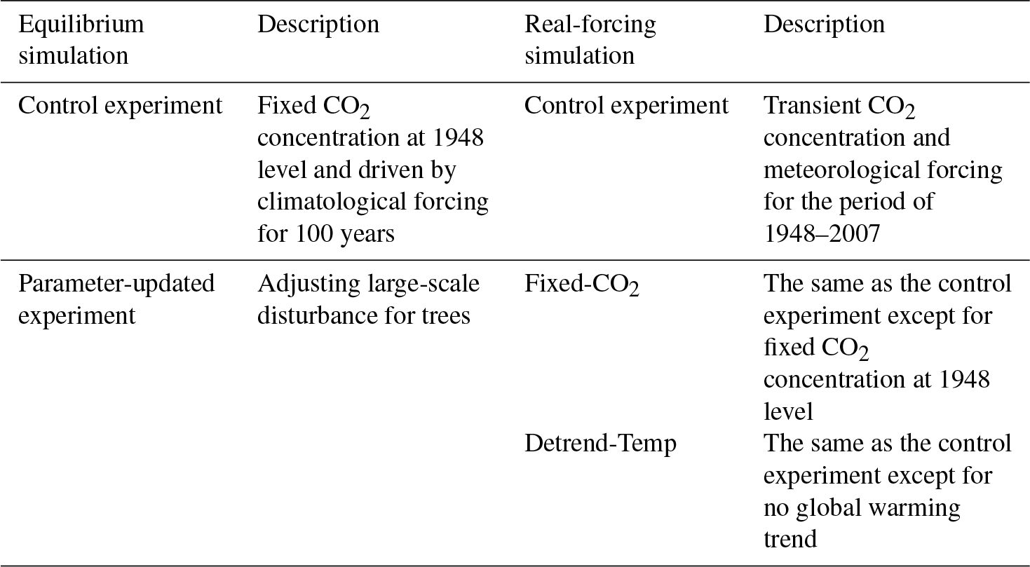
In this study, SSiB4/TRIFFID was used to simulate the global vegetation distribution and assess the sensitivity of ecosystem trends to climate and eCO₂. Two sets of simulations were performed: (1) a 100-year quasi-equilibrium simulation driven by climatological forcing, and (2) sensitivity simulations driven by real forcing from 1948 to 2007 (Table 1). In the first set, SSiB4/TRIFFID was driven with the climatological forcing and 1948 CO₂ concentration to reach a steady state, which was used as the initial condition in the second set of simulations.

Using the quasi-equilibrium simulation results as the initial condition, the historical meteorological forcing and yearly updated atmospheric CO₂ concentration were used to drive SSiB4/TRIFFID from 1948 to 2007. In this control simulation, we evaluated the model performance in reproducing the climatology and variability of vegetation coverage, LAI, and GPP in comparison with multiple observation-based datasets. The long-term trends were diagnosed before and after the climate regime shift of the 1980s. Furthermore, three sets of experiments were conducted to quantify the effects of environmental drivers (climate and CO₂) and vegetation competition on the ecosystem trends. These experiments were designed as following:

1. For the Fixed-CO₂ experiment, the model was driven by the same meteorological forcing as the control experiment, but CO₂ concentration was fixed at the level of 1948 (310.33 ppm). The difference between control experiment and Fixed-CO₂ indicates the eCO₂ effect.

2. For the Detrend-Temp experiment, the mean warming trend over each 10^∘ of latitude, from 1948 to 2007, was subtracted in this experiment. Then, the detrended temperature along with other meteorological forcing and annually varying CO₂ concentration were used to drive the model. Subtraction of Detrend-Temp from the control experiment isolates the effect of global warming.

3. For the climate variability experiment, subtraction of both Fixed-CO₂ and Detrend-Temp from the control experiment was regarded as representing the effect of CV.

2.3 Data

A SSiB vegetation and soil map is used as the preliminary initial condition for the quasi-equilibrium simulation. Three-hourly meteorological forcing data from 1948 to 2007 (Sheffield et al., 2006) are used for this study. The observation-based LAI and GPP products (Zhu et al., 2013; Xiao et al., 2014; Jung et al., 2009) are used to validate and calibrate the model to produce proper vegetation spatial distribution and temporal variability.

2.3.1 Initial condition for equilibrium simulation

There are different ways to initialize the surface condition for the quasi-equilibrium simulation. Based on our previous study (Zhang et al., 2015), we set up the initial condition using the SSiB vegetation map and SSiB vegetation table, which are based on ground survey and satellite-derived information (Dorman and Sellers, 1989; Xue et al., 2004; Zhang et al., 2015) with 100 % occupation at each grid point for the dominant PFT and zero for other PFTs.

2.3.2 Meteorological forcing data

The Princeton global meteorological dataset version 1 for land surface modeling (Sheffield et al., 2006) is used to drive SSiB4/TRIFFID for the period of 1948–2007. This dataset is constructed by combining a suite of global observation-based datasets with the National Centers for Environmental Prediction/National Center for Atmospheric Research (NCEP/NCAR) reanalysis starting from 1948 (http://hydrology.princeton.edu/data/pgf/, last access: 3 July 2011). The spatial resolution is 1^∘ × 1^∘ and temporal interval is 3-hourly. This dataset includes surface air temperature (K), pressure (Pa), specific humidity (g kg⁻¹), wind speed (m s⁻¹), downward shortwave radiation flux (W m⁻²), downward longwave radiation flux (W m⁻²), and precipitation (mm day⁻¹). Its 60-year mean climatology with 3 h intervals from 1 January to 31 December was generated to drive quasi-equilibrium simulation.

2.3.3 Observation-based data

Two satellite-derived global land cover maps are used to evaluate the vegetation distribution in both quasi-equilibrium and real-forcing simulations. The Global Land Cover (GLC) database for the year 2000 (Bartholome et al., 2002) is used and was derived from SPOT (Satellite Pour l'Observation de la Terre) at a spatial resolution of about 1 km. This dataset provides a global map with one consistent legend, as well as regional maps with separate legends containing more detail for certain regions. For instance, tundra is not included in the global legend but is included in the regional product for northern Eurasia (Bartalev et al., 2003). The regional land cover maps (download from http://forobs.jrc.ec.europa.eu/products/glc2000/glc2000.php, last access: 23 August 2017) are used to calculate the land cover fraction by counting the percentage of each PFT in a 1^∘ grid, then are merged to form a global land cover fraction map. Other than GLC2000, the land cover type climate modeling grid (CMG) product (MCD12C1), which is derived using the same algorithm that produces the V051 global 500 m land cover type product (MCD12Q1) from the observation input of Terra and Aqua on board the Moderate Resolution Imaging Spectroradiometer (MODIS), is also used as a reference (Friedl et al., 2010). The MODIS-MCD12C1 product provides land cover fraction at the spatial resolution of 0.05^∘, which is then converted to 1^∘ resolution. SSiB4/TRIFFID only includes primary land cover types, while both GLC2000 and MODIS International Geosphere-Biosphere Programme (IGBP) have more sub-level classes. For easy comparison of the distribution of dominant vegetation types with different products, we hierarchically combine the GLC2000 and the MODIS IGBP classifications with the SSiB4/TRIFFID PFTs.

To assess the climatology, variation, and trends of simulated LAI, two widely used LAI products were used as references in this study: the Global Inventory Modelling and Mapping Studies (GIMMS) LAI (refer to LAI3g, the third generation; Zhu et al., 2013) was downloaded from https://ecocast.arc.nasa.gov/data/pub/gimms (last access: 1 July 2014). A neural network algorithm was trained to using the Advanced Very High Resolution Radiometer (AVHRR) GIMMS NDVI3g (covering the period July 1981 to December 2011) and best-quality Terra MODIS LAI (covering the period 2000 to 2009) for the overlapping period (2000–2009). Then, the trained neural network algorithm was used to generate a corresponding LAI dataset at 15-day temporal resolution and 1∕12^∘ spatial resolution for the period from July 1981 to December 2011. The Global Land Surface Satellite (GLASS) LAI was downloaded from http://www.bnu-datacenter.com (last access: 18 February 2014). The GLASS LAI was generated from AVHRR reflectance (1982–1999) and MODIS reflectance (2000–2012) (Xiao et al., 2014). The GLASS LAI provides observations at 8-day temporal resolution and 1 km spatial resolution for the period from 1982 to 2012. Both datasets have general consistence in LAI spatial distribution; however, GIMMS shows 25 % of the vegetated areas are greening during 1982 to 2009, whereas GLASS LAI shows 50 % (Zhu et al., 2016). GIMMS and GLASS LAI, and the meteorological forcing data for overlap period (1982 to 2007), were resampled to 1^∘ spatial resolution and a monthly temporal interval.

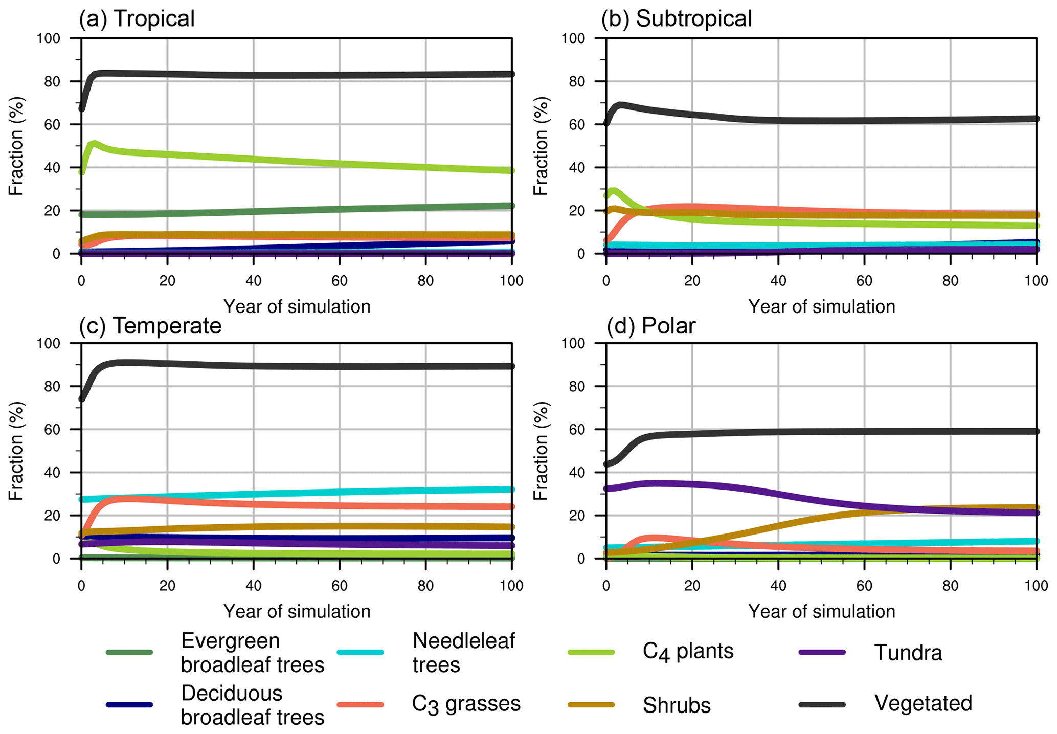
Figure 1 Fractional coverage of each plant functional type in typical climate zones in the equilibrium experiment.

SSiB4/TRIFFID GPP was evaluated using the FLUXNET model tree ensemble (MTE) GPP, which was downloaded from https://www.bgc-jena.mpg.de/geodb/projects/Data.php (last access: 7 March 2017). The FLUXNET-MTE GPP was upscaled from FLUXNET observations of carbon dioxide flux to the global scale using the machine learning technique MTEs. This method was trained to predict site-level GPP based on remote sensing indices, climate and meteorological data, and information on land use (Jung et al., 2009). This dataset provides global monthly mean GPP at 0.5^∘ spatial resolution for the period from 1982 to 2011. The FLUXNET-MTE GPP was resampled to 1^∘ spatial and monthly temporal resolution.

3 Results

3.1 Vegetation initial conditions

The DGVM's initial conditions for long-term simulations are obtained from a quasi-equilibrium solution in a long-term simulation using the climatological forcing as presented in Sect. 2.3.2. The effect of large-scale disturbance (LSD) on regulating tree fraction over the savanna areas is also investigated. The parameter for LSD is tuned to generate a reasonable tree cover distribution there.

3.1.1 Quasi-equilibrium simulation

DGVMs require initial conditions for a number of state variables. DGVMs normally take 50–1000 years' simulation under specified meteorological forcing to reach this steady state (Bonan and Levis, 2006; Zeng et al., 2008). Since our purpose was to generate the initial condition for the decadal simulations, we applied a shortcut to reach the quasi-equilibrium coexistence of PFTs under the climatological forcing. We started the model from a SSiB 1^∘ dominant vegetation map (Xue et al., 2004), with 100% occupation of the dominant PFT and zero for other PFTs at each grid point. The 1948–2007 averaged meteorological forcing along with 1948 CO₂ concentration were used to drive SSiB4/TRIFFID for 100 years. SSiB4/TRIFFID is a water, energy, and carbon balanced model. Plant expansion and biotic properties such as vegetation height and LAI are constrained by carbon allocation. FRAC links the carbon accumulation within plants and intra-species competition via a system of the Lotka–Volterra equations (Cox, 2001). In the first 10 years of the simulation, most PFTs' FRACs change rapidly but then take decades to reach a steady state (Fig. 1). To qualify the steady state, we define quasi-equilibrium status as occurring when the rate of change of vegetation fraction is less than 2 % of the mean vegetation fraction, over the last 10 years of simulation. The result shows 100-year spin-up time is sufficient for our model. Overall, in the tropical areas (23.5^∘ S–23.5^∘ N), C₄ plants and evergreen broadleaf trees are of mixed dominance and coexistent with C₃ grasses, shrubs, and deciduous broadleaf trees. The subtropical areas (23.5–35^∘ S and 23.5–35^∘ N in both hemispheres) are dominated by C₃ grasses, C₄ plants, and shrubs with similar occupation for each (∼18 %), whereas 40 % of the subtropical areas are occupied by bare land. Needleleaf trees, C₃ grasses, shrubs, and deciduous broadleaf trees are the dominant mix in the temperate zones (35–66.5^∘ S and 35–66.5^∘ N, particularly in the Northern Hemisphere). Over the polar areas (66.5–90^∘ S and 66.5–90^∘ N in both hemispheres), shrubs and tundra are of mixed dominance (Fig. 1).

Figure 2 Tree dominated areas of the (a) unchanged large-scale disturbance experiment, (b) parameter-updated experiment, and (c) GLC2000.

3.1.2 Effect of large-scale disturbance

Large-scale disturbance, such as fire, and insect outbreaks alter physical structure and/or arrangement of biotic elements with great effect. TRIFFID introduces only a global uniform and PFT-dependent parameters to represent the rate of vegetation loss caused by LSD (units: yr⁻¹). The preliminary quasi-equilibrium run shows that, under this approach, trees extended into the South American and African savanna areas (Fig. 2a), where the climate acting alone would seem to favor tree growth (Bond et al., 2005). However, major ecological disturbances vary spatially and temporally (Giglio et al., 2006). We raised the LSD coefficient (largely representing fire at this scale) from 0.004 to 0.04 (yr⁻¹) for tree PFTs that coexist with C₃ grasses and C₄ plants. With the updated setting, SSiB4/TRIFFID produced reasonable dominant tree coverage over the tropical rainforest areas (Fig. 2b) in comparison with the GLC2000 dataset (Fig. 2c). The global PFT distributions in the equilibrium run are close to the results using the real meteorological forcing.

3.2 Model evaluation of simulated vegetation distribution, LAI, and GPP

Using initial conditions derived from the equilibrium run for both biotic and abiotic variables such as FRAC, LAI, vegetation height, soil moisture, and temperature, the model is then driven with the historical meteorological forcing and yearly updated atmospheric CO₂ concentration from 1948 to 2007. In this section, the global (hereafter referring to the regions of 180^∘ W to 180^∘ E, 60^∘ S to 75^∘ N) distributions of the simulated FRAC, LAI, and GPP are compared to the observation-based datasets to ensure SSiB4/TRIFFID generates a reasonable spatial pattern and temporal variability of those variables, which provides a base for further assessment of the impact of external drivers on some surface variables.

3.2.1 Vegetation spatial distribution

Satellite-derived products are used to assess the model-simulated mean FRAC averaged over the last 10 years (Fig. 2). Overall, the model-simulated vegetated land covers 79.6 % of the global land surface, which is less than GLC2000 estimation (80.8 %) and higher than the MODIS estimation (79.3 %) (Fig. S1 in the Supplement). There is no human activity included in the model simulation, as such an agricultural category is not included. Therefore, in the following vegetation coverage comparison with the GLC products, simulated PFT coverage in the grid boxes with agriculture is reduced based on the GLC agriculture fraction. On this basis, the total simulated tree cover (the sum of evergreen broadleaf trees, deciduous broadleaf trees, and needleleaf trees) is 28.8 %, close to 29.8 % in GLC2000. The evergreen broadleaf trees in the Amazon, central Africa, and southeast Asia, deciduous broadleaf trees in southeast North America, and needleleaf trees in the high to midlatitudes of North America and Eurasia are reasonably predicted. SSiB4/TRIFFID simulates 12.7 % C₃ grass occupation, which is slightly higher than 11.9 % in GLC2000, with reasonable simulation in the midlatitudes in both hemispheres such as the central US, Eurasian steppes, South America, south and east Africa, and east Australia. The model simulates 10.1 % natural C₄ plants, compared to 7.9 % in GLC2000. The discrepancy could be partially attributed to the absence of C₄ plants in some GLC2000 regional maps (such as southeast Asia). The global GLC2000 map is assembled from these regional maps. In fact, a satellite-based physiological model simulation estimated 13.9 % of C₄ plant coverage with no agriculture category (Still et al., 2003). In the SSiB4/TRIFFID prediction without excluding agricultural land, the C₄ plants cover 13.5 %, close to Still et al.'s (2003) estimation. C₄ plants are primarily located in South American and African savanna areas, the Indian subcontinent, southeast Asia, the southeast US, and northern Australia. The model simulates 15.9 % shrubs and tundra occupation, which is close to 16.7 % in GLC2000, with shrubs primarily located in the semi-arid areas in both hemispheres and the pan-Arctic area, while tundra is located in the pan-Arctic area and Tibetan Plateau (Fig. 3, and also see vegetation fractional distribution in Fig. S2).

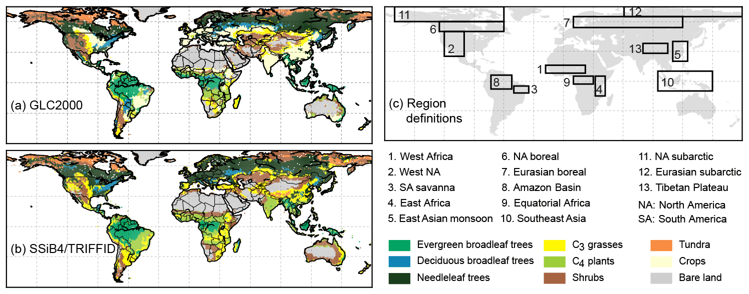
Figure 3 Dominant vegetation type comparison between (a) GLC2000 and (b) SSiB4/TRIFFID, and (c) region definitions.

3.2.2 Leaf area index

This section discusses the spatial and temporal correlations between the simulations and observations and compares with other model results. Since other published studies on this subject have not excluded agricultural areas when evaluating LAI and GPP simulation, to make our results comparable with others, the agricultural areas are not subtracted. In fact, the difference between the results with and without the exclusion of agriculture area for our results is less than 0.01.

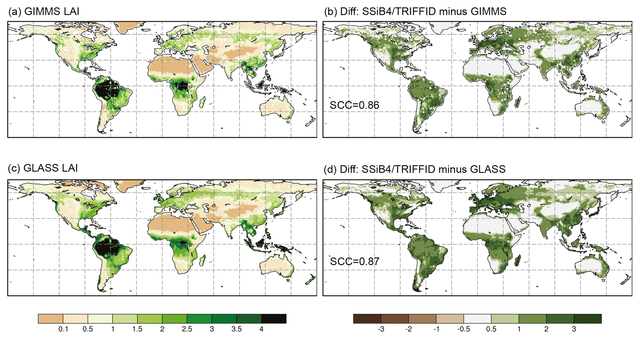
Figure 4 The 1982–2007 average leaf area index comparison for (a) GIMMS LAI, (c) GLASS LAI, and difference between SSiB4/TRIFFID and (b) GIMMS and (d) GLASS. SCC indicates the spatial correlation coefficient between model simulation and satellite-derived datasets.

SSiB4/TRIFFID produces a similar global LAI pattern compared to both the GIMMS and GLASS products, confirmed by global spatial correlation coefficients of 0.86 (GIMMS, p<0.05) and 0.87 (GLASS, p<0.05), and above 0.74 (P<0.05) against both observations over the Northern Hemisphere (Fig. 4). Previous studies reported spatial correlation coefficients between models and GIMMS LAI over the globe and Northern Hemisphere in the range of 0.44–0.77 and 0.21–0.61, respectively (Murray-Tortarolo et al., 2013; Mahowald et al., 2016). The latter study reported that in general DGVMs tended to overestimate global average LAI by 0.69±0.44 units calculated based on the table in Mahowald et al. (2016). SSiB4/TRIFFID produces ∼0.95 units higher global averaged LAI than the satellite-derived data. The absence of nitrogen limitation in the model could contribute to the overestimation.

Figure 5 The 1982–2007 average gross primary production comparison for (a) FLUXNET-MTE GPP and (b) difference between SSiB4/TRIFFID and FLUXNET-MTE GPP. SCC indicates the spatial correlation coefficient.

3.2.3 Gross primary production

The spatial correlation coefficient between model and FLUXNET-MTE GPP is 0.93 (P<0.05) (Fig. 5). Anav et al. (2015) reported less than 0.8 correlation against FLUXNET-MTE GPP for multi-model comparison. Over the globe, SSiB4/TRIFFID simulates 151 Pg C yr⁻¹, greater than the FLUXNET-MTE average of 122 Pg C yr⁻¹. However, our simulation was still within the range of 130–169 Pg C yr⁻¹ reported by Anav et al. (2015) and 111–151 Pg C yr⁻¹ reported by Piao et al. (2013). In addition to our model's deficiencies (such as lack of N limitation), the lack of CO₂ fertilization during the MTE model training may have contributed to an underestimation in the FLUXNET-MTE GPP.

3.3 Simulated vegetation temporal variability

3.3.1 Vegetation temporal variability during 1982–2007 and its comparison to observation-based data

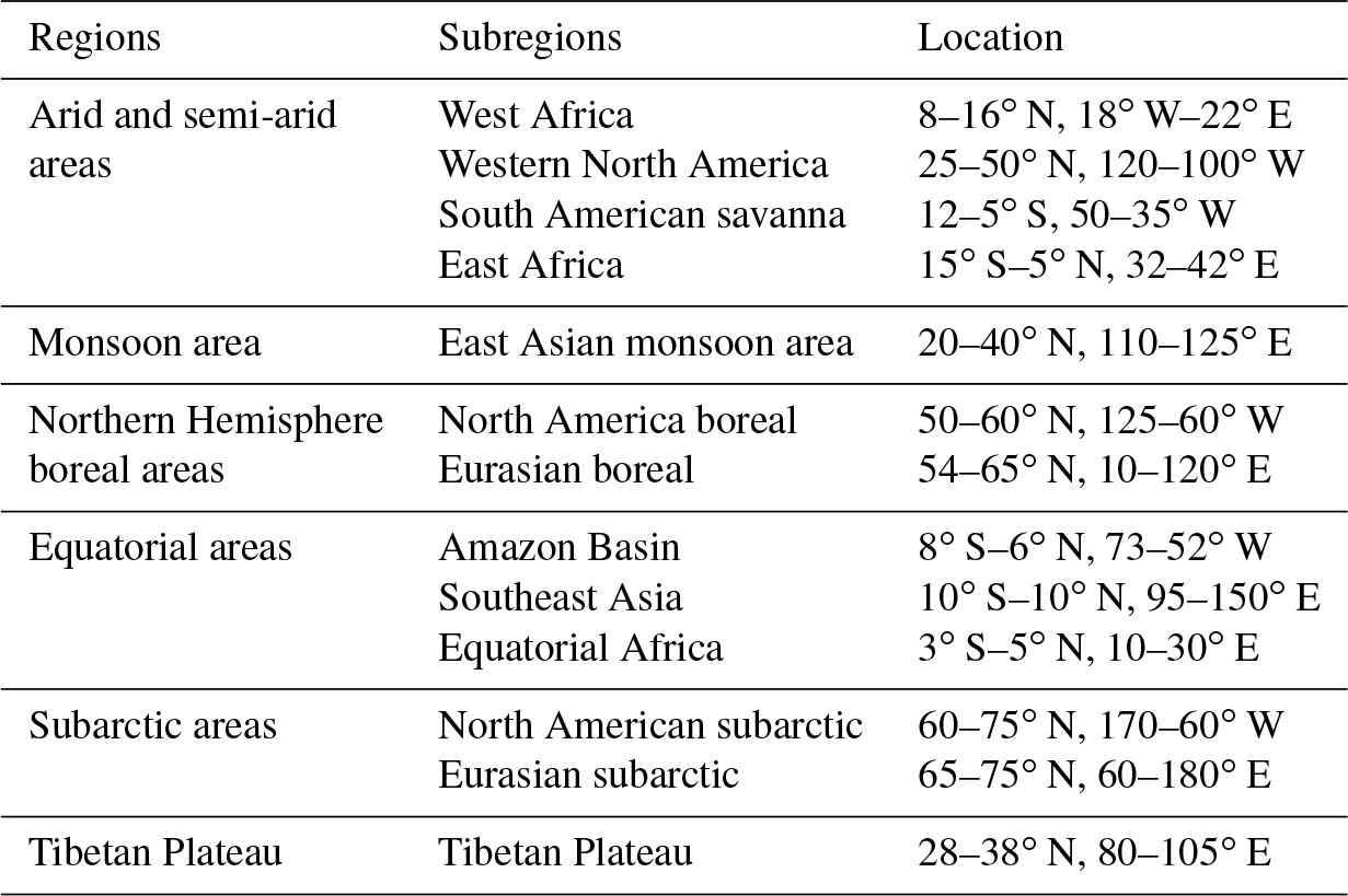
Model performance in predicting temporal variability has been less evaluated in previous studies on ecosystem trend detection and attribution (Ichii et al., 2013; Piao et al., 2013; Zhang et al., 2015). However, performance in estimating LAI and GPP trends and variability has been found to vary among models (Murray-Tortarolo et al., 2013; Piao et al., 2013; Anav et al., 2015; Zhu et al., 2017). To better assess model performance in this regard, we select 13 subregions associated with different regional climate and land cover conditions (Table 2). Although the MTE excludes CO₂ fertilization during its model training, FLUXNET-MTE GPP still incorporates variability at different scales associated with climate variability and is widely used by the community for model evaluation. Both annual LAI and GPP correlation coefficients are calculated over the period of 1982–2007.

Globally, the correlations for annual mean LAI between the SSiB4/TRIFFID and the satellite-based products are 0.58 (P<0.05) for GIMMS and 0.64 (P<0.05) for GLASS. The correlation for annual GPP is 0.59 (P<0.05) between the SSiB4/TRIFFID and FLUXNET-MTE GPP. Regionally, LAI correlations over west Africa are 0.79 (P<0.05) with GIMMS and 0.77 (P<0.05) with GLASS (Fig. 6), and GPP correlation is 0.80 (P<0.05) with FLUXNET-MTE GPP in that region. For other semi-arid areas in western North America, South American savanna areas, and east Africa, the simulated LAI significantly matches at least one of the two reference datasets with correlation in the range of 0.46–0.58 (P<0.05). The simulated GPP correlations with FLUXNET-MTE GPP are in the range of 0.63–0.70 (P<0.05). The LAI over the forested areas is better correlated to GLASS LAI, while GPP is only significantly corrected to FLUXNET-MTE GPP over the boreal forests. Over the cold regions (subarctic and Tibetan Plateau), SSiB4/TRIFFID matches the reference data in a varying range of 0.46–0.74 (P<0.05) for LAI and 0.49–0.72 (P<0.05) for GPP.

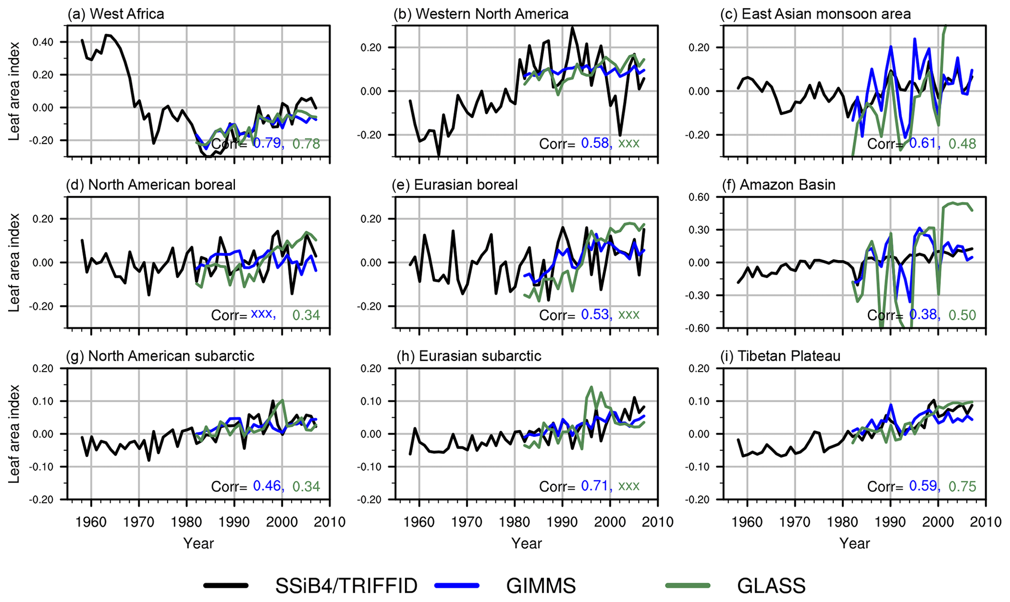
Figure 6 Comparison of standardized LAI anomalies between simulation and observations for nine subregions. Corr indicates the interannual correlation coefficient simulated (in black) LAI against the GIMMS (in blue) and the GLASS (in green). Only significant values (P<0.1) are shown, whereas non-significant values are masked by xxx.

Distinct decadal variabilities are identified in most subregions. For instance, trends reverse sign in west Africa (from negative to positive) and western North America (from positive to negative) during the 1980s (Fig. 6). Areas with enhancement in trend slopes, such as the subarctic after the climate regime shift in the 1980s, will be discussed in detail in the next section.

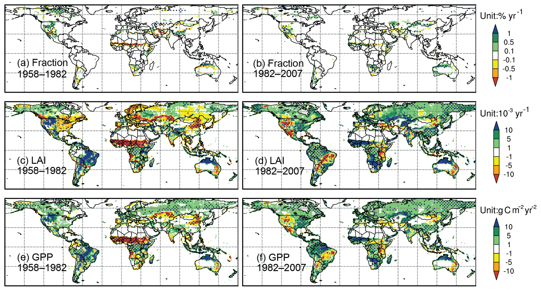
Figure 7 Trends (shaded) of (a, b) fractional coverage (units: % yr⁻¹), (c, d) LAI (units: 10⁻³ yr⁻¹), and (e, f) GPP (units: g C m⁻² yr⁻²). Panels (a, c, e) are for 1958–1982 and (b, d, f) are for 1982–2007. The dots indicate the areas with significance level at P<0.05 (Mann–Kendall test).

Generally, SSiB4/TRIFFID simulates reasonable predictions of terrestrial ecosystem climatology and variability compared to the observation-based datasets (Table 3). Compared to other DGVMs, SSiB4/TRIFFID shows above average performance in reproducing the spatial distribution but with certain bias in absolute numbers. In particular, SSiB4/TRIFFID captures the ecosystem temporal variabilities over different regions across the world, which provides a basis for pursuing the ecosystem trend detection and attribution study presented in the next section.

Table 2 Location for study areas.

3.3.2 Three major types of vegetation trend change since the 1950s

The climate regime shifted abruptly during the 1980s, giving rise to changes in ecosystem trends in many parts of the world. Here, we compare trends of FRAC, LAI, and GPP over two periods: 1958–1982 and 1982–2007. The model performance for the second period, for which satellite observations are available, is evaluated in Sect. 3.3.1. Spatial patterns of the trends are shown in Fig. 7.

Table 3 Statistics for the comparison between SSiB4/TRIFFID simulated and observation-based LAI and GPP.

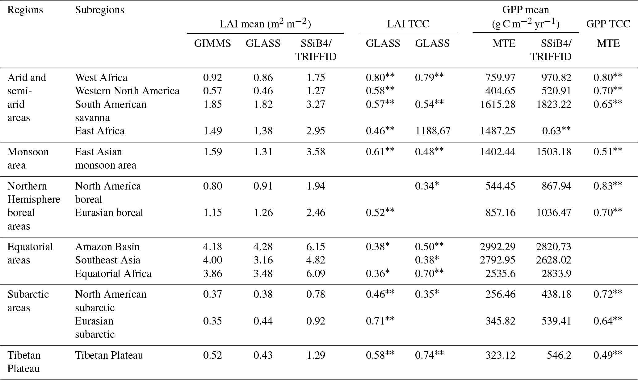
Note: ^* indicates p<0.1 and ${}^{**}$ indicates p<0.05. TCC is the temporal correlation coefficient.

At the global scale, significant vegetation trends are only found in the simulations after the 1980s. During this period, FRAC increases at the rate of 0.032 yr⁻¹. LAI has a positive trend of 0.0029 yr⁻¹, which matches very well to GIMMS' results (0.0029 yr⁻¹). GPP has a positive trend of 2.22 g C m⁻² yr⁻², within the range of 1.60–4.69 g C m⁻² yr⁻² for GPP over similar periods (Anav et al., 2015; Yue et al., 2015). In contrast to LAI and GPP, there are relatively few areas with a significant simulated FRAC trend (Fig. 7).

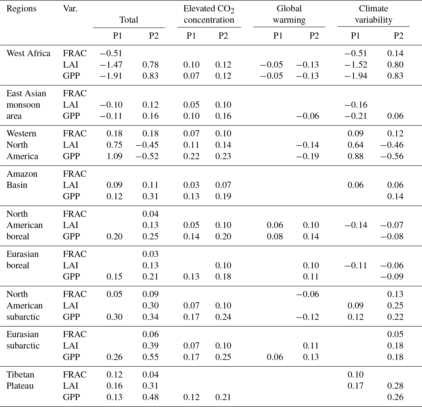
Table 4 Linear trend of vegetation FRAC, LAI and GPP changes during P1 (1958–1982) and P2 (1982–2007) in subregions^*.

^* Only significant values (P<0.1 in Mann–Kendall test) are shown. Numbers are scaled by multiplying by 10 for FRAC and by 1000 for LAI.

For the global land surface, over 40.2 % has a significant LAI trend from 1958 to 2007, and over 48.1 % has a significant GPP trend. In response to the climate regime shift during the 1980s, the terrestrial ecosystem has three major trend changes in different parts of the world after the 1980s (Table 4). (1) There is trend sign reversal from negative to positive in the East Asian monsoon area, west Africa, central Asia, and the eastern US, over 14.2 % (LAI) and 11.4 % (GPP) of the land surface. In particular, west Africa experiences the largest vegetation deterioration in the world before the 1980s, associated with LAI and GPP reductions of 0.0258 yr⁻¹ and 18.54 g C m⁻² yr⁻², respectively – approximately 10 times the trends of the global average. After the 1980s, recovery is simulated at the rate of 0.0137 yr⁻¹ and 8.02 g C m⁻² yr⁻² for LAI and GPP, respectively. (2) Trend sign reversal from positive to negative is found in western North America, South American savanna, and east Africa, which accounted for 2.9 % (LAI) and 2.7 % (GPP) of the land surface. (3) There are consistent positive trends but substantially enhanced by at least 50 % of prior period trends after the 1980s, which are found in equatorial rainforest areas, boreal forest areas, south Africa, north Australia, subarctic areas, and the Tibetan Plateau, representing over 11.7 % (LAI) and 19.3 % (GPP) of the land surface. There are also areas with consistent positive trends but no substantial change during the entire period or other types of trend change over much smaller areas. The first three major trend changes as described above will be discussed in the following sections.

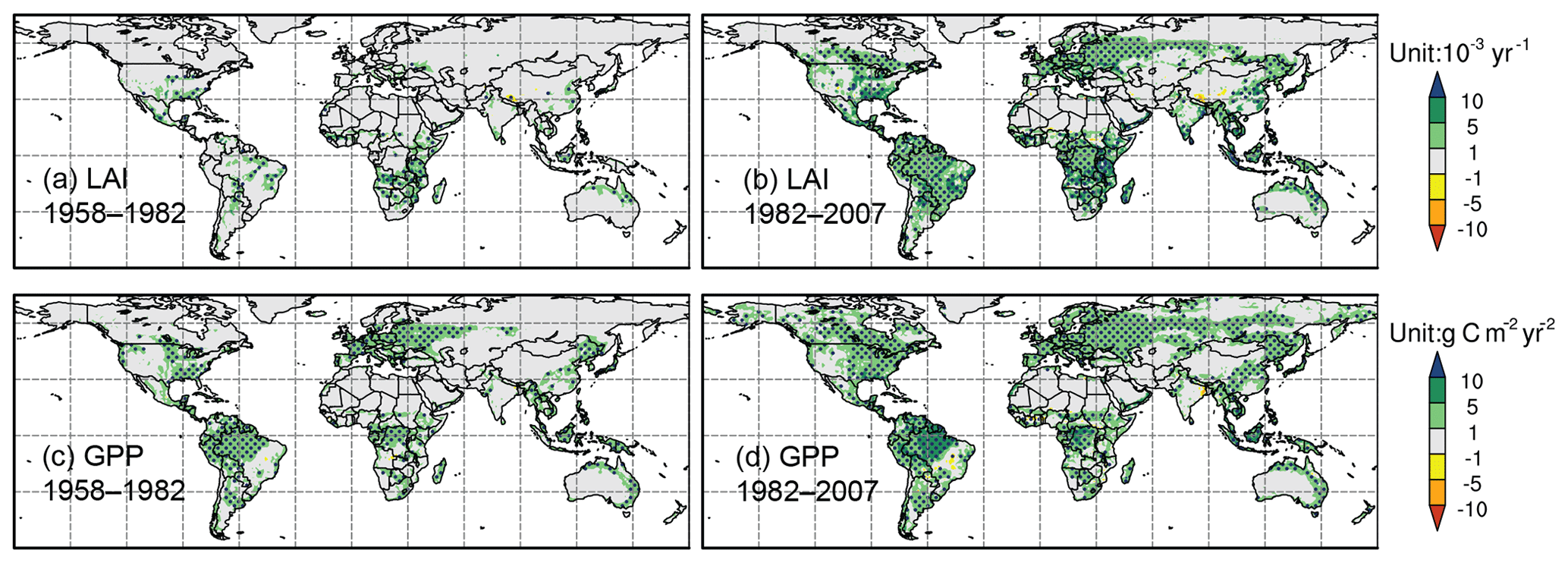
Figure 8 CO₂ effect on the trends (shaded) of (a, b) LAI (units: 10⁻³ yr⁻¹) and (c, d) GPP (units: g C m⁻² yr⁻²). Panels (a, c) are for 1958–1982 and (b, d) are for 1982–2007.

3.4 Attribution of three environmental drivers on ecosystem trends

3.4.1 Global overview of three simulated environmental drivers' effects on the ecosystem trends

Sensitivity experiments were conducted to isolate the contributions of elevated atmospheric CO₂ concentration, global warming, and climate variability. The differences between the control experiment and Fixed-CO₂ show that eCO₂ stimulated vegetation growth mainly in the equatorial areas and eastern North America, western Europe, and eastern China in the midlatitudes. Substantially enhanced positive trends are found after the 1980s for both LAI and GPP over those areas (Fig. 8). eCO₂ promoted rainforest LAI increase only after the 1980s; however, its effect on GPP appeared during the entire period. GPP is directly linked to CO₂ through the photosynthesis process, while LAI, in addition to the photosynthesis process, is also affected by respiration and carbon allocation in plants, which are influenced by both climate and eCO₂ (O'Sullivan et al., 2017).

Figure 9 Same as Fig. 8 but for warming effect.

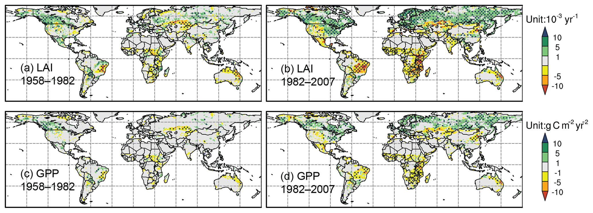
The differences between the control experiment and Detrend-Temp show that global warming has minor effects on the trends of LAI and GPP before the 1980s (Fig. 9). After the 1980s, the rapidly enhanced warming contributes positive LAI trends at high latitudes, while the GPP change seems less substantial. Meanwhile, there are negative trends due to heat stress in low latitudes, particularly in the semi-arid regions such as South American savanna, east Africa, and central Asia.

The differences between the control experiment and Fixed-CO₂ and Detrend-Temp show the CV effect, which has complex influences on the ecosystem. The CV in this study includes contribution of changes in surface pressure, precipitation, surface wind speed, downward longwave and shortwave radiation, and surface humidity, along with temperature that excludes the global warming trend. Precipitation is however found to play a dominant role. The correlation coefficients between the annual mean CV effect on LAI and GPP and annual mean precipitation at the grid points with significant CV effect are greater than 0.60 (P<0.05). Overall, the CV effect alone can explain the total FRAC trends in the control experiment (Fig. 10). Before the 1980s, CV causes LAI to decrease in East Asian monsoon areas, eastern North America, west Africa, western Europe, central Asia, Siberia, and eastern Australia. The GPP also decreases in these areas except for eastern North America, western Europe, and Siberia. In contrast, the CV effect before the 1980s leads LAI and GPP increase in the Tibetan Plateau and south Asia, western North America, South American savanna areas, east and south Africa, and northern Australia. Due to the climate regime shift, CV has produced the opposite sign to the trends of LAI and GPP in East Asian monsoon areas, central Asia, west Africa, North America, South American savanna areas, and east Africa. In some areas, such as south Africa and northern Australia, persistent precipitation increase/decrease leads to sustained positive/negative trends from the 1950s.

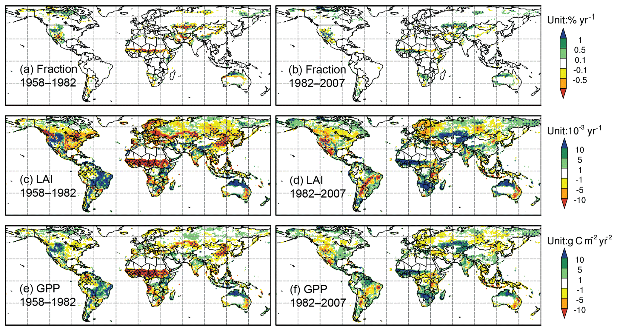
Figure 10 Same as Fig. 8 but for climate viability effect and also including the effects on fractional coverage (units: % yr⁻¹).

Overall, after the 1980s, the effects of eCO₂ and global warming have been generally enhanced, but the CV effect has exhibited distinctly different regional features before/after the 1980s over many regions in the world. The enhanced or opposite contribution of the primary driver and the changes in their relative importance on the ecosystem trends occur during the 1980s, resulting in different ecosystem responses in many regions across the world.

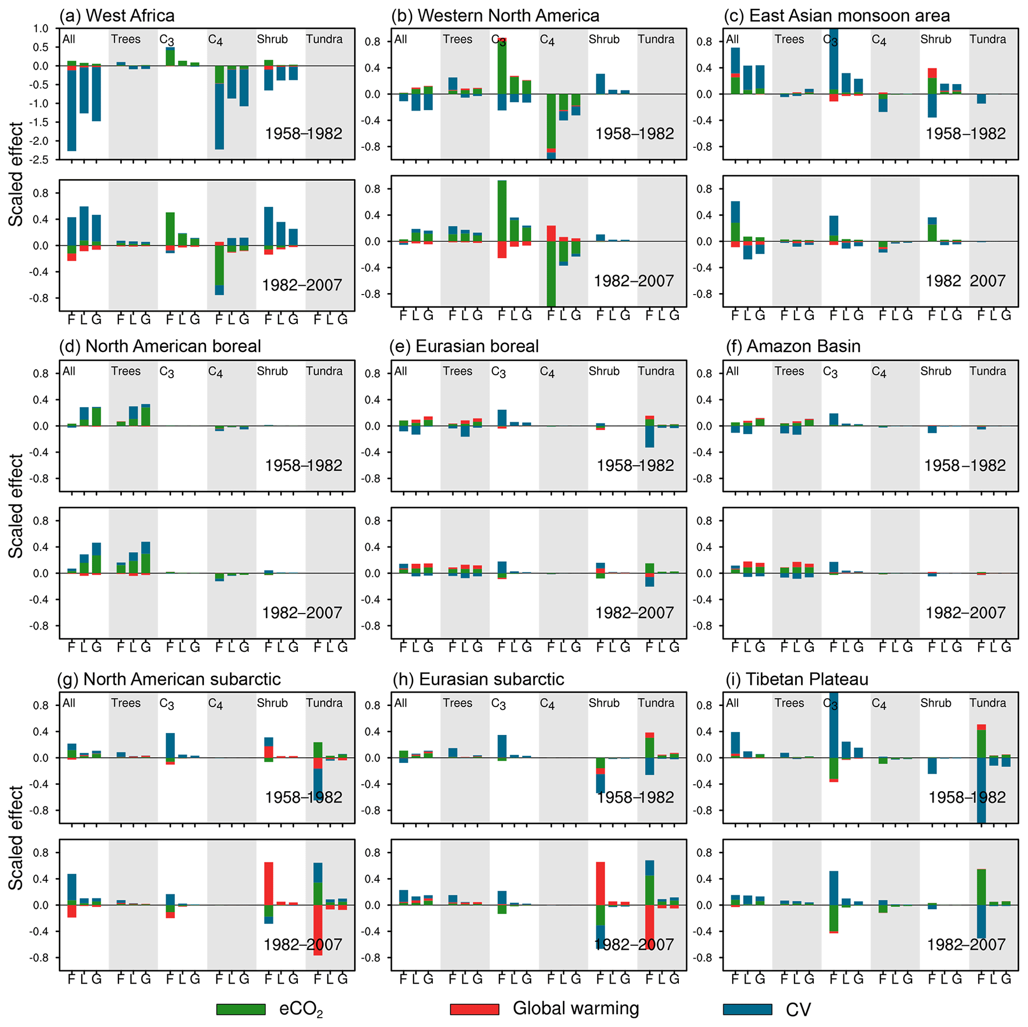
Figure 11 Contribution of each factor on FRAC (denoted as “F”), LAI (denoted as “L”), and GPP (denoted as “G”) trends over subregions. For panels (a–i), the upper sections indicate trends during 1958–1982 and lower sections indicate trends during 1982–2007. The effects of eCO₂, global warming, and CV are shown in green, red, and blue bars, separately. Each column shows the effects on all PFTs (All), trees, C₃ grasses (C₃), C₄ plants (C₄), shrub, and tundra, separately. The numbers for FRAC, LAI, and GPP are normalized by dividing the standard deviation of global average in the control experiment.

3.4.2 Dominant factor in influencing trend reversal from negative to positive in west Africa and east Asia

CV is found to be the dominant driver of the ecosystem trends in west Africa, explaining most of the LAI and GPP trends and trend changes (Fig. 11a). Before the 1980s, CV causes C₄ plants' LAI, GPP, and FRAC over the region to decrease, followed by shrubs, whereas eCO₂ caused C₃ grasses' LAI and GPP to slightly increase. Global warming shows little effect during the entire period from 1958 to 2007. The ecosystem trends in west Africa reverse from decreasing to increasing when the precipitation trend changes to increasing after the 1980s, with the major increase in C₃ grasses and shrubs over the region. A previous study using satellite data also showed recent west Africa greening is highly correlated with the precipitation increase (Herrmann et al., 2005). eCO₂ has played a role in increasing C₃ grasses' coverage since the 1950s. However, the PFT competition outcomes reduce the C₄ plant coverage over the region, mainly after the 1980s when eCO₂ has a large impact. As such, the change in regional FRAC overall within west Africa is not significant and has been compromised by positive and negative contributions of the individual PFTs after the 1980s.

Regional average trends reverse in the East Asian monsoon area because CV and eCO₂ dominate LAI and GPP trends, before and after the 1980s, respectively. Their combined effects cause trend reversal in the East Asian monsoon areas. CV contributes to decreasing trends of LAI and GPP before the 1980s but with minor effects after the 1980s, while eCO₂ has dominated the PFT LAI and GPP trends since the 1950s, which caused a significant increase in C₃ grasses and trees but significant decrease in C₄ plants (Fig. 11b). Meanwhile, enhanced global warming after the 1980s stimulates C₄ plant growth, but this effect is compromised by its detrimental effect on C₃ grasses after the 1980s. Overall, the CV and eCO₂ relative contribution change during the 1980s dominates the negative to positive trend shift in this area.

3.4.3 Dominant factor in influencing trend reversal from positive to negative in western North America

The eCO₂ effect has persistently caused LAI, GPP, and FRAC increase since the 1950s, while global warming reduced both LAI and GPP only after the 1980s. However, CV dominated the LAI and GPP trends and trend reversal in western North America by causing the dominant PFTs (C₃ grasses and shrubs) to increase/decrease before/after the 1980s (Fig. 11c and Table 5). The CV effect on FRAC change is more complex due to its different effects on LAI and GPP and FRAC expansion in C₃ and shrub PFTs after the 1980s: both C₃ and shrubs expand with LAI and GPP decrease. This discrepancy suggests that expansion might be coupled with carbon fixation less than with growth in the model. We conjecture that CV may promote vegetation expansion into some areas that are largely unvegetated, but this requires further investigation.

3.4.4 Dominant factor in influencing the enhanced positive trend in rainforest, boreal forest, subarctic, and Tibetan Plateau

eCO₂ and CV have had persistent positive impacts on tropical rainforest growth in terms of LAI and GPP since the 1950s (Fig. 11d). eCO₂ dominates the LAI and GPP trends in both periods except for the LAI positive trend before the 1980s, which is dominated by CV. LAI trend enhancement after the 1980s is associated with increased CO₂ fertilization, while GPP trend enhancement is attributed to increase in both eCO₂ and CV effects. The importance of CO₂ and CV impacts on the rainforests is confirmed by previous analyses on the trends of LAI and NDVI (Hilker et al., 2014; Zhu et al., 2016).

Table 5 Climate drivers and eCO₂ effect on the trends of FRAC, LAI, and GPP during P1 (1958–1982) and P2 (1982–2007) in subregions with regard to their regional average^1,2.

¹ Percentage trend for FRAC: trend_FRAC∕(grid total vegetated FRAC) ⋅ 100 % percentage trend for LAI and GPP: trend_var∕(grid averaged) ⋅ 100 %, where “var” stands for LAI or GPP. Units for all three variables are % yr⁻¹. ² Only significant values (P<0.05 in the Mann–Kendall test) are shown.

eCO₂ and global warming have increased LAI and GPP in North American boreal forest areas since the 1950s and caused significant positive trends over the Eurasian boreal forest area after the 1980s (Fig. 11e). However, due to CV-induced negative effects on tree LAI, no significant trend is found in regional average LAI in boreal areas before the 1980s. The LAI and GPP trend enhancement in the boreal forest areas can be attributed to the enhanced eCO₂ and global warming effects, accompanied by reduced CV negative effects after the 1980s.

North American subarctic areas have enhanced LAI and GPP positive trends after the 1980s, which were caused by the increase in eCO₂ and CV positive effects, while all three environmental drivers have effects on LAI and GPP positive trends in the Eurasian subarctic (Fig. 11f). Meanwhile, remarkable FRAC changes have been found since the 1950s. Our simulation suggests that global warming continually favored shrub invasion into tundra biomes, except in the Eurasian subarctic before the 1980s. After the 1980s, this shrubification is enhanced due to increase in the warming effect. In contrast, eCO₂ has promoted tundra expansion and shrub decline over subarctic areas since the 1950s, which mitigates the shrubification. Meanwhile, CV plays a role to help tree and C₃ grass expansion into subarctic areas and also alters the shrub and tundra competition.

Over the Tibetan Plateau (Fig. 11g), CV has dominated the positive LAI and GPP trends since the 1950s, except in the case of the GPP increase before the 1980s which is dominated by eCO₂. The positive trend enhancements for LAI and GPP after the 1980s are caused by the impact of both eCO₂ and CV. Furthermore, our simulation also suggests that CV favors C₃ grasses but harms tundra biome expansion. However, eCO₂ has the opposite effects on those PFTs, in contrast to the CVs.

4 Discussion

The spatial distribution of the dominant PFT is closely related to large-scale climate (MacDonald, 2003), and DGVMs are designed to reproduce the observed ecosystem–climate relationship. There is diverse performance in reproducing the spatial distribution and temporal variability of the ecosystems (Murray-Tortarolo et al., 2013; Piao et al., 2013; Anav et al., 2015; Zhu et al., 2017), which resulted in large discrepancies between models in identifying attributed dominant drivers of changes (Beer et al., 2010; Huntzinger et al., 2017). It is therefore important to validate the model performance in reproducing the observed ecosystem variability and spatial distribution first before using DGVMs for attribution studies. As a matter of fact, it is challenging for DGVMs to reproduce PFT coexistence, particularly for the smaller PFTs in semi-humid and semi-arid areas, as they are fragile and sensitive to climate and vulnerable to competition (Fu et al., 2006). Because of that difficulty, Zeng et al. (2008) had to introduce a specific submodel to grow temperate shrubs in the spaces unoccupied by trees and grasses. SSiB4/TRIFFID allows smaller fractions of PFTs to coexist with full competition with other PFTs (Cox, 2001). After modifying the competition coefficients in the Lotka–Volterra equation (Zhang et al., 2015) and updating large-scale disturbance parameters, it produces a reasonable global distribution of temperate shrubs and high-latitude tundra (Fig. 3). During the validation process, some parameters in SSiB4/TRIFFID have also been calibrated (Zhang et al., 2015).

With all these efforts, the SSiB4/TRIFFID-produced LAI and GPP show higher temporal correlation with observation compared to the start-of-the-art offline models in the TRENDY intercomparison project (Piao et al., 2013; Sitch et al., 2015; Zhu et al., 2016). The improvement may mainly be due to better capturing of the interannual variability by SSiB4/TRIFFID in semi-arid areas, which has been considered as dominating global interannual variability (Poulter et al., 2014; Ahlstrom et al., 2015). Meanwhile, both simulated LAI and GPP are also well correlated with reference data over the Northern Hemisphere boreal forests. Our evaluation is based on satellite-based products, which are the only sources providing global distribution at long-term periods. Although these products showed a general consistency among them, large relative uncertainties were identified over some regions (Jiang et al., 2017), which contribute to large discrepancy of interannual correlations when the simulated LAI was compared to GIMMS and GLASS LAIs (Fig. 6). It should be pointed out that the GPP simulation over the rainforests exhibit inconsistency with the FLUXNET-MTE GPP. We consider that the missing CO₂ fertilization in FLUXNET-MTE GPP could be a predominant limitation to its GPP there. By and large, SSiB4/TRIFID's performance suggests this model is appropriate to be applied for the attribution study.

SSiB4/TRIFFID simulates increased LAI and GPP after the 1980s (Fig. 8), which is confirmed by observation and the TRENDY models' simulation (Anav et al., 2013 for GPP; Piao et al., 2013 and Zhu et al., 2016 for LAI). These increases are considered to be responding to elevated atmospheric CO₂ concentrations and warming surface temperature in high latitudes (Zhu et al., 2016). Some areas with decreased LAI and GPP are due to decrease in precipitation and/or increase in stress due to warming temperature in low latitudes (Anav et al., 2013; Zhu et al., 2016). Our study, however, further estimates large-scale trends in all three aspects, i.e., carbon fixation (GPP) and vegetation growth (LAI), as well as expansion, instead of focusing only on one aspect, such as the LAI trend in Zhu et al. (2016). Our results also reveal different LAI and GPP responses to the environmental changes (Figs. 8–10), indicating LAI and GPP are involved in different processes as discussed in O'Sullivan et al. (2017). The results suggest that GPP is more directly linked to atmospheric CO₂ (Fig. 8).

In SSiB4/TRIFFID, net CO₂ assimilation is proportional to the gradient of atmosphere and leaf CO₂ concentration (Zhan et al., 2003; also see the Supplement). Hence, the elevated atmospheric CO₂ concentration leads to an increase in GPP, while LAI in TRIFFID is related to carbon allocation and competition between PFTs. As such, LAI is not only affected by the atmospheric carbon concentration but also other processes, such as phenological processes and the percentage collocated carbon for growth. Therefore, GPP is more sensitive to the change in atmospheric carbon concentration compared to LAI. Integrated analysis and observation with multiple variables, such as LAI and GPP, are required to improve the understanding of vegetation biochemical process and climate effect on ecosystem changes.

The competition between PFTs within a grid box contributes to the ecosystem trend discussed above. Our analysis with grid points has shown intensive interactions between PFTs. For instance, shrubs are found to expand into tundra ecosystems (Fig. 11f), which is linked to climate change (Myers-Smith et al., 2015), particularly to global warming (Tape et al., 2006; Elmendorf et al., 2012) and precipitation (Martin et al., 2017). The response to eCO₂ of a particular PFT not only depends on its own physiological and morphological characteristics but is also determined by the interactions that arise with other PFTs, competing for the same resources (Fig. 11a). Field experiments reported that the differential growth and competitiveness responses of C₃ grasses and C₄ plants to eCO₂ are complex and under debate (Leakey et al., 2009; Lee, 2011; Miri et al., 2012). In this paper, we have discussed the competition between C₃ and C₄, and its contribution to the trend change. It seems under the elevated atmospheric CO₂ concentration scenario C₃ grasses show enhanced competitive ability over C₄ plants at regional scale (Fig. 11b). Different responses of the coexisting PFTs to the climate regime shift either enhance or mitigate the environmental drivers' contribution at grid-averaged scale.

Furthermore, our results show that the boundary between the Sahara and Sahel have experienced significant variation since the 1950s. Based on the observed precipitation data and the precipitation/NDVI correlation, Thomas and Nigam (2018) suggested a Sahara desert expansion starting from the 1950s. Our results are in agreement at large with the Thomas and Nigam (2018) study but also with substantial differences in the rate at two different climate regimes. A comprehensive discussion on this issue is out of the scope of this paper and will be addressed in a separate paper.

5 Conclusion

This work employs a biophysical dynamic vegetation model (SSiB4/TRIFFID) to explore the responses of the terrestrial ecosystem to climate variability, global warming, and elevated atmospheric CO₂ concentration during 1948–2007. SSiB4/TRIFFID is evaluated by available satellite data in simulating the land surface carbon fixation, and plant growth and competition. We have shown that the SSiB4/TRIFFID model can simulate the vegetation and temporal variability for the period 1982–2007. A series of sensitivity experiments is then conducted to detect the ecosystem trends and attribute the trends to elevated atmospheric CO₂ concentration (eCO₂), global warming, and CV.

The effects of the external drivers on the ecosystem trends manifest distinct spatial and temporal characteristics. For the global land surface, over 40.2 % has a significant LAI trend and over 48.1 % had a significant GPP trend during the 1958–2007 period. In responding to the climate regime shift during the 1980s, the terrestrial ecosystem had three major changes in different parts of the world after the 1980s. Over 14.2 % (LAI) and 11.4 % (GPP) of the land surface, primarily located in the East Asian monsoon area, west Africa, central Asia, and the eastern US, had trend sign reversal from negative to positive. In contrast, trend reversal from positive to negative is found in western North America, South American savanna, and east Africa, which accounted for 2.9 % (LAI) and 2.7 % (GPP) of the land surface. Meanwhile, there are consistent positive trends substantially enhanced in equatorial rainforest areas, boreal forest areas, south Africa, north Australia, subarctic areas, and the Tibetan Plateau, representing over 11.7 % (LAI) and 19.3 % (GPP) of the land surface, respectively.

In general, the major types of trend change are attributed to the changes in relative contributions of environmental drivers and, consequently, the changes in the dominant driver, or changes in the dominant driver's “direction” in its effect (enhancing or suppressing) on the ecosystem. The eCO₂ stimulates vegetation growth through fertilization effects mainly in the equatorial areas, as well as eastern North America, western Europe, and eastern China in the midlatitudes. The rapidly enhanced global warming after the 1980s contributes positive LAI trends at high latitudes, while the GPP change seems less substantial. Meanwhile, there are negative trends in LAI and GPP due to the heat stress in low latitudes. CV dominates the variability of FRAC, LAI, and GPP in the semi-humid and semi-arid areas. The overall effects on the ecosystem are the integrated contribution of all environmental drivers.