the Creative Commons Attribution 4.0 License.
the Creative Commons Attribution 4.0 License.
 | 30 Oct 2019
Maximum power of saline and fresh water mixing in estuaries
Zhilin Zhang
Hubert Savenije
According to Kleidon (2016), natural systems evolve towards a state of maximum power, leading to higher levels of entropy production by different mechanisms, including gravitational circulation in alluvial estuaries. Gravitational circulation is driven by the potential energy of fresh water. Due to the density difference between seawater and river water, the water level on the riverside is higher. The hydrostatic forces on both sides are equal but have different lines of action. This triggers an angular moment, providing rotational kinetic energy to the system, part of which drives mixing by gravitational circulation, lifting up heavier saline water from the bottom and pushing down relatively fresh water from the surface against gravity; the remainder is dissipated by friction while mixing. With a constant freshwater discharge over a tidal cycle, it is assumed that the gravitational circulation in the estuarine system performs work at maximum power. This rotational flow causes the spread of salinity inland, which is mathematically represented by the dispersion coefficient. In this paper, a new equation is derived for the dispersion coefficient related to density-driven mixing, also called gravitational circulation. Together with the steady-state advection–dispersion equation, this results in a new analytical model for density-driven salinity intrusion. The simulated longitudinal salinity profiles have been confronted with observations in a myriad of estuaries worldwide. It shows that the performance is promising in 18 out of 23 estuaries that have relatively large convergence length. Finally, a predictive equation is presented to estimate the dispersion coefficient at the downstream boundary. Overall, the maximum power concept has provided a new physically based alternative for existing empirical descriptions of the dispersion coefficient for gravitational circulation in alluvial estuaries.
- Article
(6382 KB) - Full-text XML
- Companion paper
- BibTeX
- EndNote


Estuaries are water bodies in which rivers with fresh water meet the open sea. The longitudinal salinity difference causes a water level gradient along the estuary. As a result, the water level at the limit of salt intrusion is set up several centimeters above sea level (about 0.012 times the estuary depth). Therefore, the hydrostatic forces from the seaside and riverside have different lines of action (a third of the setup apart). Since the hydrostatic forces at the seaside and the salinity limit are equal but opposed, this difference in the lines of action triggers an angular moment (a torque) that drives the gravitational circulation, whereby fresh water near the surface flows to the sea and saline water near the bottom moves upstream (Savenije, 2005). This density-driven gravitational circulation is one of the two most significant mixing mechanisms in alluvial estuaries; the other is the tide-driven mixing mechanism that can be dominant in the wider (downstream) part of estuaries (Fischer et al., 1979).
Kleidon (2016) described the concept of maximum power in the Earth system, implying that freely evolving systems perform work and dissipate energy at maximum power (close to or at the Carnot limit). Using this concept, gravitational circulation is assumed to take place at the maximum power limit. Earlier, the maximum power concept was used to solve saline and fresh water mixing as in a thermodynamic equilibrium system (Zhang and Savenije, 2018). It assumed that in thermodynamic terms, the freshwater flux maintains a potential energy gradient, triggering fresh and saline water mixing processes that work at depleting this gradient. Because the strength of the mixing in turn depends on this gradient, there is an optimum at which the mixing process performs at maximum power. It did not, however, account for the energy loss associated with this mixing process. The equation obtained appeared to have an analytical solution of a straight line for the longitudinal salinity distribution. Although this is not correct, it can be seen as a first order approximation, which agrees with earlier theoretical work by Hansen and Rattray (1965), who developed their theory for the central region of the salt intrusion length at which the salinity gradient is at its maximum and dominated by density-driven mixing. However, this approximate solution was not fully satisfactory for simulating the salinity distribution.
In contrast to the earlier work by Zhang and Savenije (2018), in this paper friction is taken into account. The available free energy by the angular moment is converted into work (mixing the saline and fresh water against the force of gravity) and the associated frictional dissipation. In the following sections we shall derive a new equation for density-driven mixing, which appears to compare well with observations in a range of alluvial estuaries.
Kleidon (2016) presented several examples for the application of the maximum power limit on nonthermal energy conversions. In one example, a fluid is kept in motion by an accelerating force that provides kinetic energy to the system. The velocity of the fluid is slowed down by friction and the remainder is converted into another form of energy. If the velocity is too large, the friction is large and energy dissipation dominates, then the power of the force to generate work is limited. In contrast, if the velocity is too small, the power is not enough to generate work. Hence, there is an optimum value for the product of the force and velocity to produce maximum useful energy. Estuaries are comparable to this system. In this article, we apply the maximum power concept to gravitation circulation generated by a longitudinal density gradient.
Traditionally, the empirical Van der Burgh (VDB) method has worked very well to describe the mixing in alluvial estuaries, leading to predictive equations to describe the salinity intrusion in alluvial estuaries (Savenije, 2005, 2012). The VDB method takes account of all mixing mechanisms, including density-driven (gravitational) circulation and tide-driven mixing. For application of the VDB method, there are two parameters that need to be calibrated, the empirical Van der Burgh coefficient K and the dispersion coefficient at the downstream boundary D0. This method has performed surprisingly well around the world and has been used in this paper as the benchmark model for comparison with the maximum power approach.
In an estuary, the cross-sectional average hydrostatic forces have equal values along the estuary axis. Over a segment, the forces are opposed but working on different lines of action due to the density gradient in the upstream and downstream directions. As a result, they exert an angular moment (torque) Macc that drives the gravitational circulation, performing as accelerating torque. The velocity of the gravitational circulation kept in motion by this accelerating torque is slowed down by a friction moment Mfric, which is the product of the associated friction force and its arm. The remainder Mex drives the circulation and executes work against gravity (Fig. 1). Hence, the balance in steady state in a segment is
The moment due to the friction against the circulation is expressed as
with Ffric being the friction force (N) and lm the scale of the arm of the frictional forces in meters.
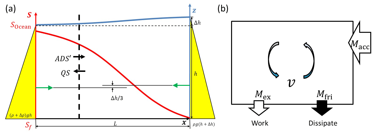
Figure 1(a) Systematic salt transport in estuaries, with the seaside on the left and the riverside on the right. The water level (in blue) has a slope as a result of the salinity distributions (in red). The hydrostatic forces on both sides have different lines of action that trigger the gravitational circulation, providing an accelerating moment Macc to the system. (b) A box model displaying the moment balance in open estuarine systems.
The friction force during the dispersive circulation is expressed as
where τ is the shear stress (N m−2) and O is the contact area (m2). Estuarine mixing has two length scales: a vertical and a horizontal one. The horizontal length scale is the tidal excursion E, which is the distance a water particle travels on the tide; the vertical length scale is the depth h, over which saline water is moved upward to the surface and over which relatively fresh water is moved downward to the bottom. Since the process of gravitational mixing is essentially to move the saline water up and the fresher water down, the contact area for the resistance against this movement is determined by the depth (h) and the width (B). Following that reasoning, O is assumed equal to Bh. Meanwhile, the circulation cell has a dimension constrained by the depth. The circular movement hence has a diameter of the depth and lm, the horizontal arm between the vertical frictional forces, is of the order of magnitude of the depth.
2.1 Maximum power condition in estuaries
Because the velocity of the dispersive gravitational circulation is small, the mixing flow is assumed to be laminar. The shear stress is typically a function of flow velocity (v): τ=ρqv, with ρ being the density (kg m−3) and q being a laminar resistance (m s−1). The latter is assumed to be proportional to the tidal velocity amplitude (), where T is the tidal period in seconds. Hence, the flow velocity representing the gravitational circulation is
Power is defined by the product of a force and its velocity. The power of torque (angular moment) is defined as the product of the moment and its angular velocity. Hence, the power is defined as
where ω is the angular velocity or the rotational speed (s−1). Figure 2 illustrates how the execution moment and the flow velocity vary. If the working moment is too large and causes fast mixing flow, the energy dissipation is large and diminishes the flow velocity. If it is too small, the mixing would also be suboptimal. In analogy with Kleidon (2016), the product of the working moment and the flow velocity has a well-defined maximum. The maximum power (MP) is then obtained by . Hence, the optimum values of the execution moment Mex,opt and the flow velocity vopt are
and
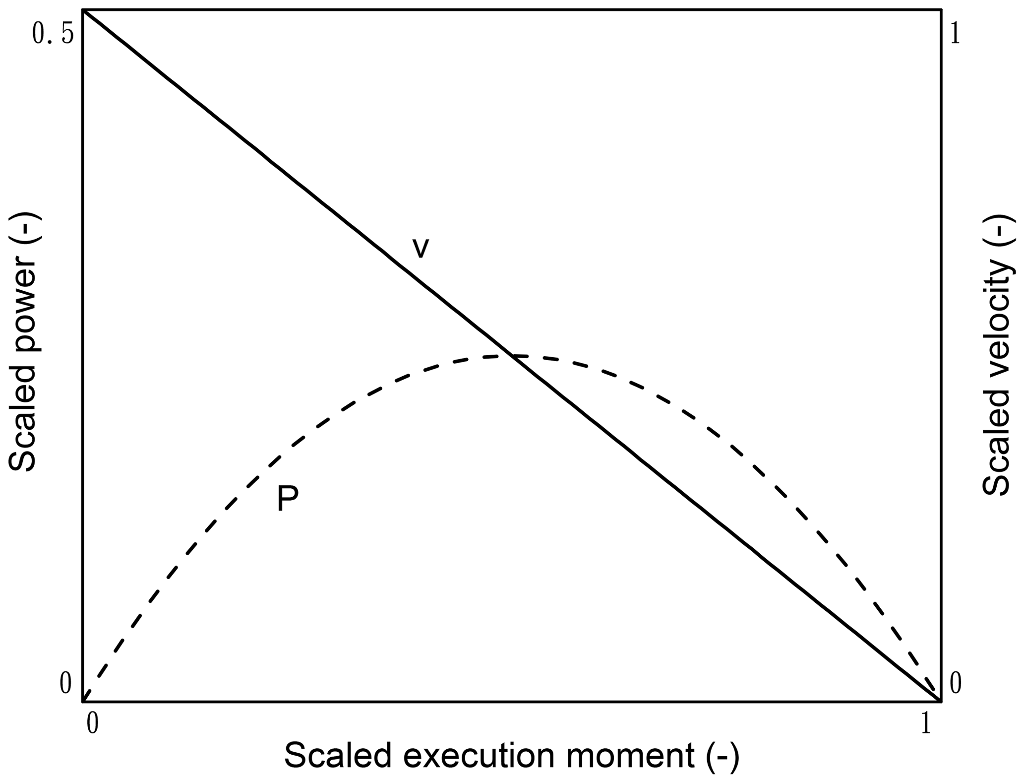
Figure 2Sketch of the sensitivity of the exchange flow velocity v to the working moment Mex.
Here, the accelerating force (Facc) that produces the angular moment is the hydrostatic force obtained by integrating the hydraulic pressure over the depth:
where ρ0 is the density of the seaside (kg m−3).
The accelerating moment has an arm Δh∕3 (Savenije, 2005). The water level gradient according to the balance of the hydrostatic pressures results in
where x is the distance in meters. Density is a function of salinity (S; psu): , where ρf is the density of the fresh water (kg m−3) and cS () is the saline expansivity (psu−1).
Subsequently, the accelerating moment due to the density gradient driving gravitational circulation over a tidal cycle can be described as
where E is the horizontal length scale of the gravitational circulation in meters.
In steady state, the one-dimensional advection–dispersion equation averaged over the cross section and over a tidal cycle reads (Savenije, 2005, 2012)
where Q is the freshwater discharge (m3 s−1), A (=Bh) is the cross-sectional area (m2), and D is the dispersion coefficient (m2 s−1). The positive direction of flow is in the upstream direction.
Accordingly, with , the optimum velocity is
Assuming that the steady state over a tidal cycle is driven mainly by the accelerating moment, especially in the upstream part where tidal mixing is relatively small and this gravitational circulation (Dg) is proportional to the dispersive residual velocity (Dg∝voptE),
This equation indicates that the dimensionless dispersion coefficient is proportional to the root of the estuarine Richardson number NR:
where υ is the tidal velocity amplitude (m s−1). The Richardson number describes the balance between the potential energy of the fresh water flowing into the estuary () and the kinetic energy of the tidal flood flow (ρυ2AE∕2) (Fischer et al., 1979; Savenije, 2005; Zhang and Savenije, 2017).
2.2 Analytical solution for the dispersion equation
Equations derived from the maximum power concept are obtained along the estuary axis, and hence they can be used at any segment along the estuary. Then, Eq. (13) becomes
where C3 is a factor (psu−1 m s−1) and all local variables are a function of x.
The following equations are used for the tidal excursion and width in alluvial estuaries:
where δH is the tidal damping rate (m−1) and b is the geometric convergence length of the width in meters. A smaller b value implies stronger convergence (a stronger funnel shape). The subscript “0” represents parameters at the geometric boundary condition (x=x0).
At the boundary, Eq. (15) is given by
Substitution of Eqs. (16)–(18) into Eq. (15) gives
with .
Differentiating Dg with respect to x and using the steady-state Eq. (11) results in
The cross-sectional area A is given by
where a is the convergence length of the cross-sectional area in meters.
Substituting Eq. (21) into Eq. (20) and in analogy with Kuijper and Van Rijn (2011) and Zhang and Savenije (2017), the solution of the linear differential Eq. (20) is
with .
At the salinity intrusion limit (x=L), Dg=0, resulting in
The solution for the longitudinal salinity distribution yields
This solution is comparable to other research. It is similar to Savenije (2005) if Ω=0, although his solutions had an empirical Van der Burgh coefficient K. In addition, the solution is the same as Kuijper and Van Rijn (2011) if a equals b, which implies that the depth is constant along the estuary.
With these new analytical equations, the dispersion and salinity distribution can be obtained using the boundary conditions (D0 and S0).
The boundary condition is often taken at the geometric inflection point (x=x0) if the estuary has one. The compilation of the Muar estuary in Fig. 3 is an example. Vertical dashed lines display the inflection point. If there is no inflection point such as in the Landak estuary, the boundary condition is taken at the estuary mouth (x0=0). Figure 3 demonstrates that the geometry of the alluvial estuaries fits well on a semilogarithmic plot, supporting the exponential functions of the cross section and the width (Eqs. 17 and 21).
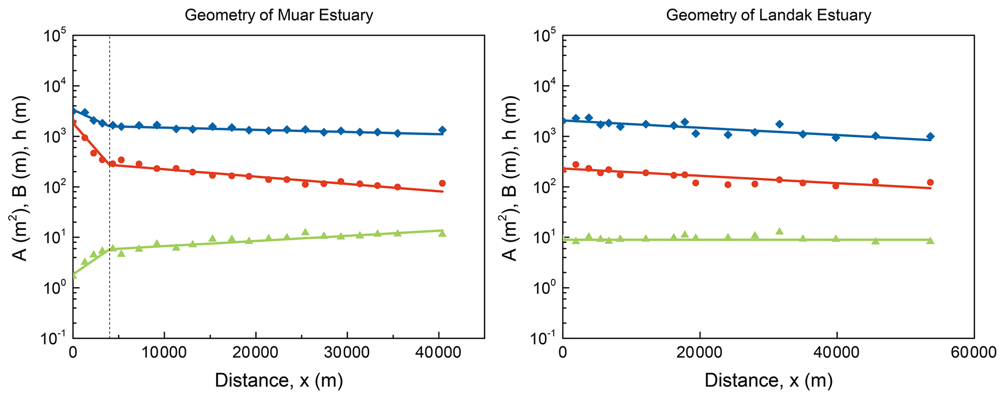
Figure 3Semilogarithmic presentation of estuary geometry, comparing simulations (lines) to the observations (symbols), including cross-sectional area (blue diamonds), width (red dots), and depth (green triangles). Vertical lines display the inflection point.
Subsequently, Eq. (24) is used by confronting the solution with observations using appropriate boundary conditions. Appendix B shows how the new equation based on the maximum power concept works in 23 estuaries around the world. The Van der Burgh (VDB) method (Savenije, 2005), which has been proven to perform well in alluvial estuaries in different parts of the world and includes all mixing mechanisms, is used for comparison. Density-driven gravitational circulation is one part of the dispersive actions in estuaries. Hence, the total dispersive process from the Van der Burgh method (DVDB) must be larger than the gravitational dispersion from the maximum power method (DMP). The general geometry and measurements follow the database from Savenije (2012), Gisen (2015), and Zhang and Savenije (2017). The information on the VDB and MP methods is summarized in Table 1. Often there is more than one salinity observation in a certain estuary (labeled by alphabet), and the observation chosen from each estuary with a star-marked label is represented in Appendix B.
Table 1Summary of application results using two methods.
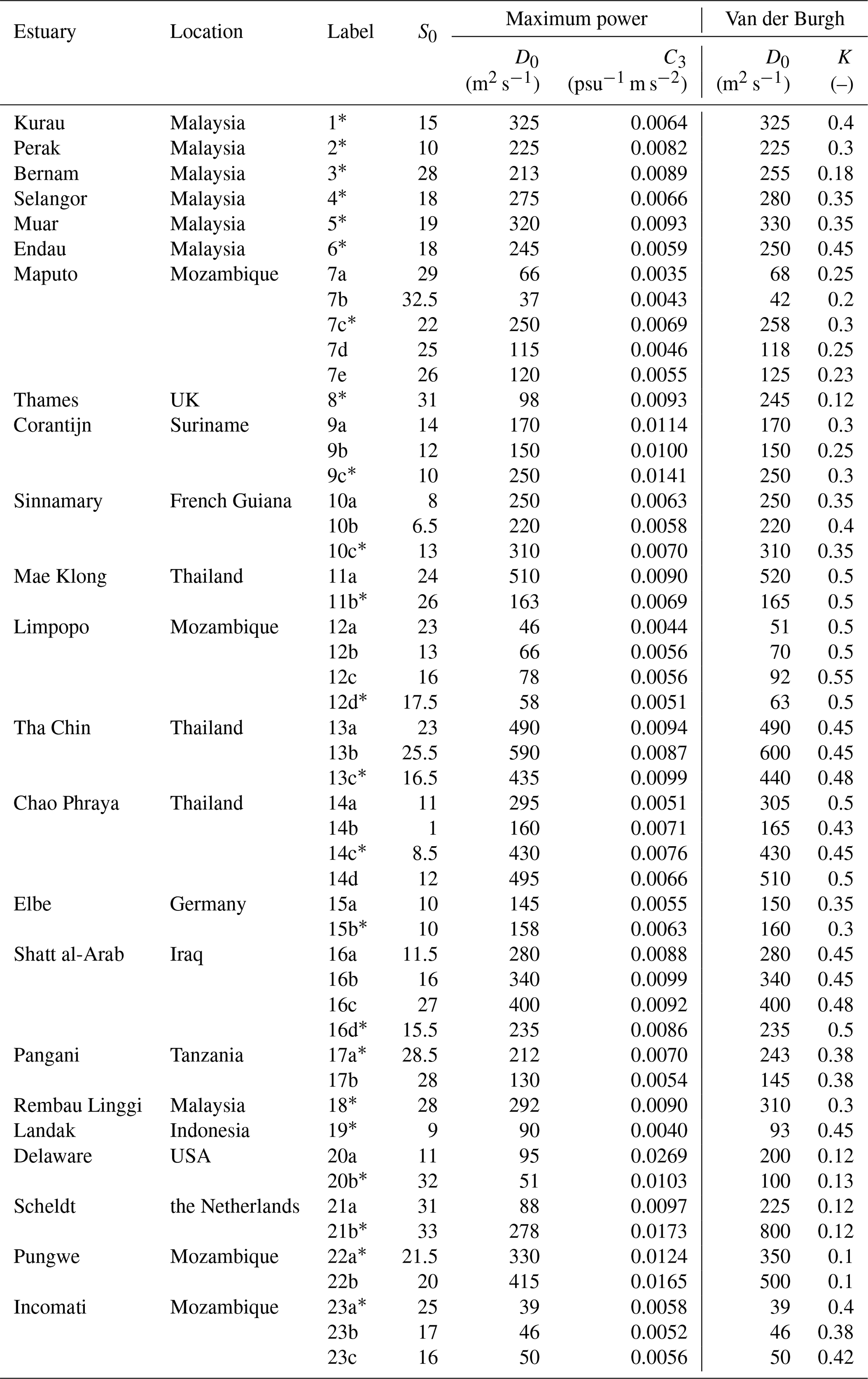
∗ Note: the observation chosen from each estuary is represented in Appendix B.
It can be seen that the simulated curves by the new MP method do not perform well in the wider part of the estuary (particularly upstream from the inflection point) where tidal mixing is dominant. However, the salinity observations can be very well simulated landward from the inflection point in most estuaries. In the Bernam, the Pangani, the Rembau Linggi, and the Incomati estuaries, the central part, where DMP closely approach DVDB, is well represented. In these estuaries, the calibration is slightly lower than the observations near the intrusion limit. In general, the dispersion derived with the maximum power method declines upstream from the inflection point in agreement with the total dispersion of the empirical Van der Burgh method, which corresponds to the theory that gravitational circulation is the dominant mixing mechanism in the landward part of these estuaries, especially in the center regime (e.g., Hansen and Rattray, 1965).
However, in the Thames (no. 8), the Delaware (no. 20), the Scheldt (no. 21), and the Pungwe (no. 22), the new approach seems not to work for both the salinity and dispersion profiles. In these estuaries tide-driven mixing is dominant. Figure 4 shows the relation between the geometry and the Van der Burgh coefficient K values. It can be seen that estuaries with poor performances by the MP approach have lower b∕B0 and K values. However, not all estuaries with a strongly convergent geometry perform poorly, revealing that the geometry is not the only effect. According to the expression of Ω, tidal damping can play a role. In wide estuaries with strong convergence, the role of gravitational circulation is insufficient to describe the mixing. Tidal mixing processes such as lateral circulation, tidal pumping, and tidal shear are dominant. The Scheldt, with preferential ebb and flood channels, is a case in point (Nguyen et al., 2008). In addition, the Corantijn (no. 9) is considered uncertain because it has a low b∕B0 value and contains few observations.
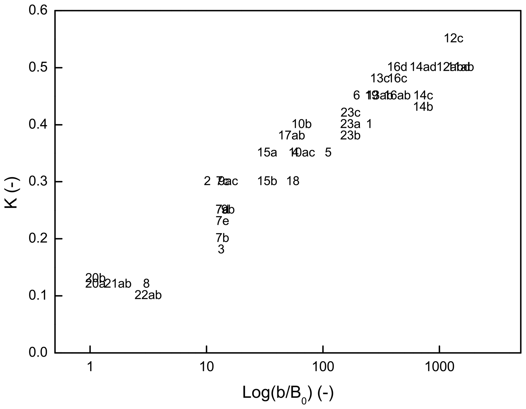
Figure 4Comparison of the geometry to the Van der Burgh coefficient. Numbers show the labels of the estuaries.
Overall, the maximum power approach in open systems is a useful tool to understand the mixing processes in most estuaries. In the upstream part where the effect of the tide is small, gravitational circulation plays the main role. There, the MP approach yields good results. At the same time, the predictions upstream are more relevant for water users. Where the salinity is high, it is less relevant since the water is already too saline for domestic or agricultural use.
This study provides an approach to define the dispersion coefficient due to gravitational circulation, which is proportional to the product of the dispersive velocity of the gravitational circulation and the tidal excursion length (which is the longitudinal mixing length over which one particle travels during a tidal cycle). The dispersive velocity actually represents the strength of the density-driven mechanism. Based on the maximum power method (Eq. 15), the dispersive velocity can be described as
Hence, the dispersive flow due to gravitational circulation strengthens with larger freshwater discharge (more stratification) and weakens with stronger tide E (less stratification).
Using the calibrated dispersion coefficient at the inflection point, C3 can be calculated. Except in estuaries with poor performance, C3 values range from to with an average of (the relative standard deviation equals 0.26). Using the average C3 value to predict Dg0 (Eq. 18), Fig. 5 shows how the predictive equation performs. It reveals that almost all the data fall within a factor of 2, and the maximum power method underestimates the dispersion coefficient in estuaries with low b∕B0 values (in red) in which gravitational circulation is not enough to describe the total dispersive processes. Finally, the R2 value of the regression in Fig. 5 equals 0.86. Considering all the uncertainties in the measurement, C3 equalling is a promising approximation to predict Dg0.
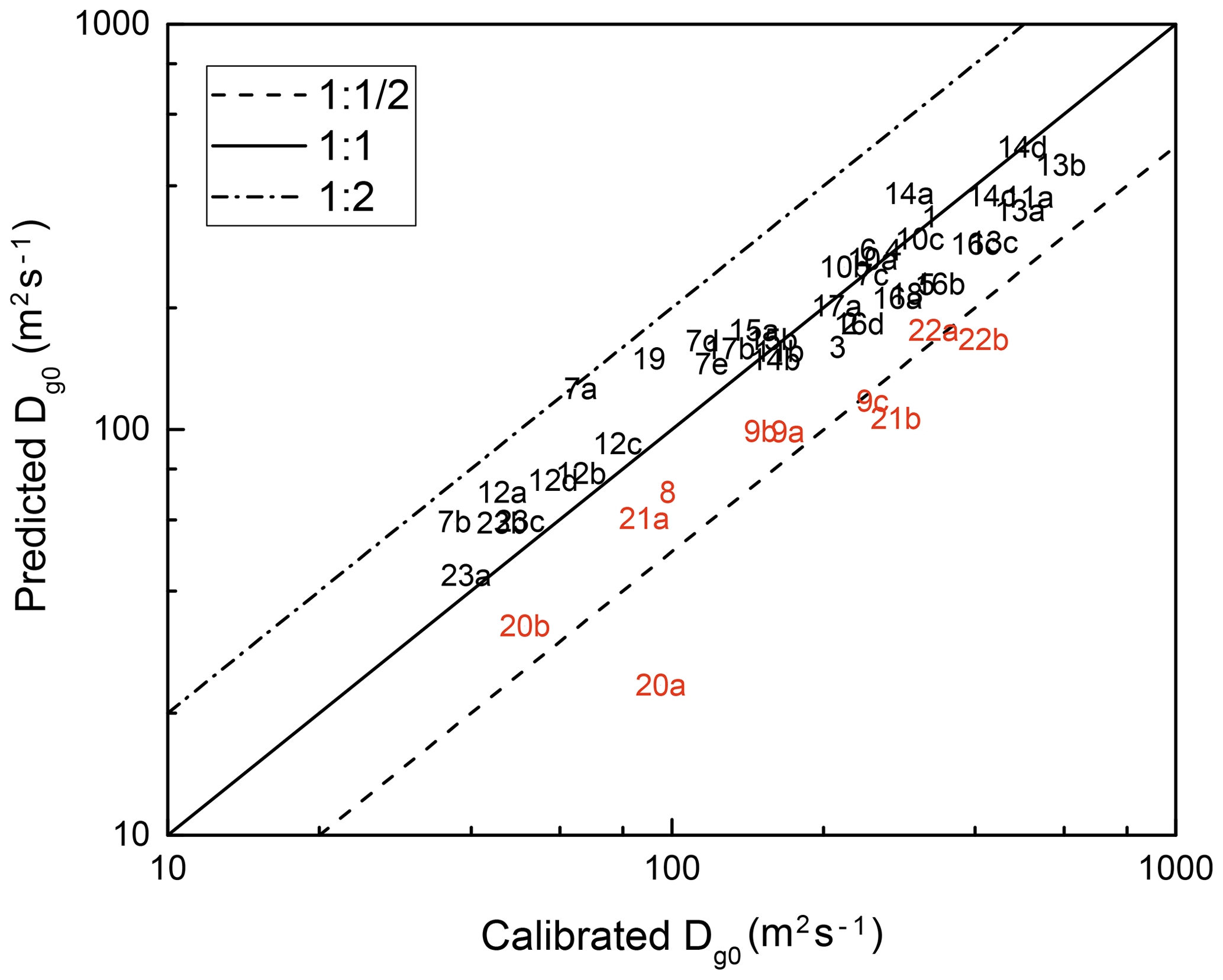
Figure 5Comparison of calibrated and predicted Dg0 values by using . Labels in red, indicating that the estuaries have relatively poor performance, are presented for validation.
Finally, there is uncertainty about the timescale of reaching this optimum. If this timescale is longer than the tidal period, then such an optimum is not reached. In a low-flow situation, however, which is the critical circumstance for salt intrusion, the variation of the river discharge is slow (following an exponential recession). If the timescale of flow recession is large compared to the timescale of salinity intrusion then it is reasonable to assume that the maximum power optimum is approached.
The fact that the MP method works well for density-driven mixing but not for tide-driven mixing, whereas the VDB method works well for the combination of the two, offers an excellent opportunity for the combination of the two methods. The VDB method requires two parameters: the K of Van der Burgh and the dispersion coefficient at the downstream boundary D0, while the MP method only requires the downstream boundary condition Dg0. The dispersion of the VDB method, which deals with all mixing processes, should therefore always be larger than the dispersion determined by the MP method. Hence, the MP method can be used to impose an additional constraint on the calibration of the VDB method, which reduces the potential equifinality between K and D0. Appendix B shows the result of this mixed calibration approach: the dispersion of the VDB method is always higher than the dispersion of the MP method, and the resulting fit by the VDB method is quite acceptable.
This combined approach also allowed for more accurate predictive equations as derived before. The correlation between K and the estuary geometry is strong, as shown in Fig. 4. This relation can be used as a predictive equation for K. Also, the predictive equation for Dg0 is powerful, as can be seen in Fig. 5, except for very wide estuaries where calibration remains necessary and where this predictive equation can be used as a 1st-order estimate for D0.
An estuary is an open system that has a maximum power limit when the accelerating source is stable. This study has described a moment balance approach to nonthermal systems, yielding a new Eq. (15) for the dispersion coefficient due to the density-driven gravitational circulation. It shows that the dispersive action is closely related to the salinity, the freshwater discharge, the tide, and the estuarine width. This equation has been used to solve the tidal average salinity and dispersion distributions together with the steady-state Eq. (11). The maximum power model has then been validated with 50 salinity observations in 23 estuaries worldwide and compared with the Van der Burgh method. Generally, the new equation is a helpful tool to analyze the salinity distribution in alluvial estuaries, providing an alternative solution for the empirical Van der Burgh method in estuaries where gravitational circulation is the dominant mixing mechanism. A predictive equation for dispersion at the geometric boundary has also been provided.
As can be seen in Appendix B, the gravitational dispersion is always smaller than the total effective dispersion obtained by the Van der Burgh method. In all estuaries that have a wide mouth, we see substantial tide-driven dispersion, most probably as a result of interacting preferential ebb and flood channels. This tide-driven mechanism is responsible for the (sometimes pronounced) concave slope of the salinity curve near the mouth. In the middle reach where the salinity gradient is steepest, density-driven dispersion is dominant and equals the total effective dispersion. Further upstream, where the salinity gradient gradually tends to zero and the estuary becomes narrower, we see the tide-driven circulation again becoming more prominent. This is in the part of the estuary where the width-to-depth ratio becomes smaller and the bank shear results in more pronounced lateral velocity gradients and hence more pronounced lateral circulation. The tide-driven mixing mechanism is particularly strong in macro-tidal estuaries such as the Thames, the Scheldt, the Pungwe, and the Delaware.
This study is a further development of the paper by Zhang and Savenije (2018), which also considered gravitational circulation based on the maximum power concept but which did not consider the associated frictional dissipation. The approach followed in this paper maximizes the work performed by the driving gravitational torque to mix the fresh and saline water, taking account of the energy dissipation associated with this mixing. As a result, we found a solution that combines well with the empirical Van der Burgh method, providing an additional constraint for its calibration. Because the total mixing of the Van der Burgh method (DVDB) should be larger than the gravitational mixing of the maximum power concept (DMP), the calibration of the Van der Burgh method is more constrained. As a result, the Van der Burgh K and the dispersion at the boundary D0 can be correlated with physically observable parameters through analytical equations, which makes the Van der Burgh method a more powerful predictive model that can be applied to alluvial estuaries worldwide. More reliable observations in other estuaries are suggested to validate these maximum power and Van der Burgh methods.
About the data, all observations are available on the website at http://salinityandtides.com/ (Savenije, 2012).
This Appendix represents the application in 23 estuaries around the world of the maximum power method for determining the dispersion coefficient and the salinity distribution using Eqs. (22) and (24), compared to salinity observations. The empirical Van der Burgh method is included as a reference.

Figure B1Left: Application of the analytical solution from the maximum power method (solid lines) to observations (symbols) for high water slack (HWS, in red) and low water slack (LWS, in blue). The green line shows the tidal average (TA) condition. Dash dot lines reflect applications of the Van der Burgh method. Vertical dash lines display the inflection point. Right: Simulated dispersion coefficient using different methods.
HS conceptualized and supervised the study. ZZ executed the research and prepared the article.
The authors declare that they have no conflict of interest.
This article is part of the special issue“Thermodynamics and optimality in the Earth system and its subsystems (ESD/HESS inter-journal SI)”. It is not associated with a conference.
The first author is financially supported for her PhD research by the China Scholarship Council.
This paper was edited by Stefan Hergarten and reviewed by Axel Kleidon and one anonymous referee.
Fischer, H. B., List, E. J., Koh, R. C. Y., Imberger, J., and Brooks, N. H.: Mixing in inland and coastal waters, Academic Press, New York, USA, https://doi.org/10.1016/C2009-0-22051-4, 1979. a, b
Gisen, J. I. A.: Prediction in ungauged estuaries, PhD thesis, Delft University of Technology, Delft, the Netherlands, https://doi.org/10.4233/uuid:a4260691-15fb-4035-ba94-50a4535ef63d, 2015. a
Hansen, D. V. and Rattray Jr., M.: Gravitational circulation in straits and estuaries, J. Mar. Res., 23, 104–122, 1965. a, b
Kleidon, A.: Thermodynamic foundations of the Earth system, Cambridge University Press, London, UK, https://doi.org/10.1017/CBO9781139342742, 2016. a, b, c, d
Kuijper, K. and Van Rijn, L. C.: Analytical and numerical analysis of tides and salinities in estuaries; part II: salinity distributions in prismatic and convergent tidal channels, Ocean Dynam., 61, 1743–1765, https://doi.org/10.1007/s10236-011-0454-z, 2011. a, b
Nguyen, A. D., Savenije, H. H. G., van der Wegen, M., and Roelvink, D.: New analytical equation for dispersion in estuaries with a distinct ebb-flood channel system, Estuar. Coast. Shelf S., 79, 7–16, https://doi.org/10.1016/j.ecss.2008.03.002, 2008. a
Savenije, H. H. G.: Salinity and tides in alluvial estuaries, Elsevier, Amsterdam, the Netherlands, https://doi.org/10.1016/B978-0-444-52107-1.X5000-X, 2005. a, b, c, d, e, f, g
Savenije, H. H. G.: Salinity and tides in alluvial estuaries, 2nd Edn., available at: http://salinityandtides.com/ (last access: 28 October 2019), 2012. a, b, c, d
Zhang, Z. and Savenije, H. H. G.: The physics behind Van der Burgh's empirical equation, providing a new predictive equation for salinity intrusion in estuaries, Hydrol. Earth Syst. Sci., 21, 3287–3305, https://doi.org/10.5194/hess-21-3287-2017, 2017. a, b, c
Zhang, Z. and Savenije, H. H. G.: Thermodynamics of saline and fresh water mixing in estuaries, Earth Syst. Dynam., 9, 241–247, https://doi.org/10.5194/esd-9-241-2018, 2018. a, b, c
- Abstract
- Introduction
- Moment balance for an open estuary system
- Empirical validation and discussion
- Combination of the MP and VDB methods
- Conclusions
- Data availability
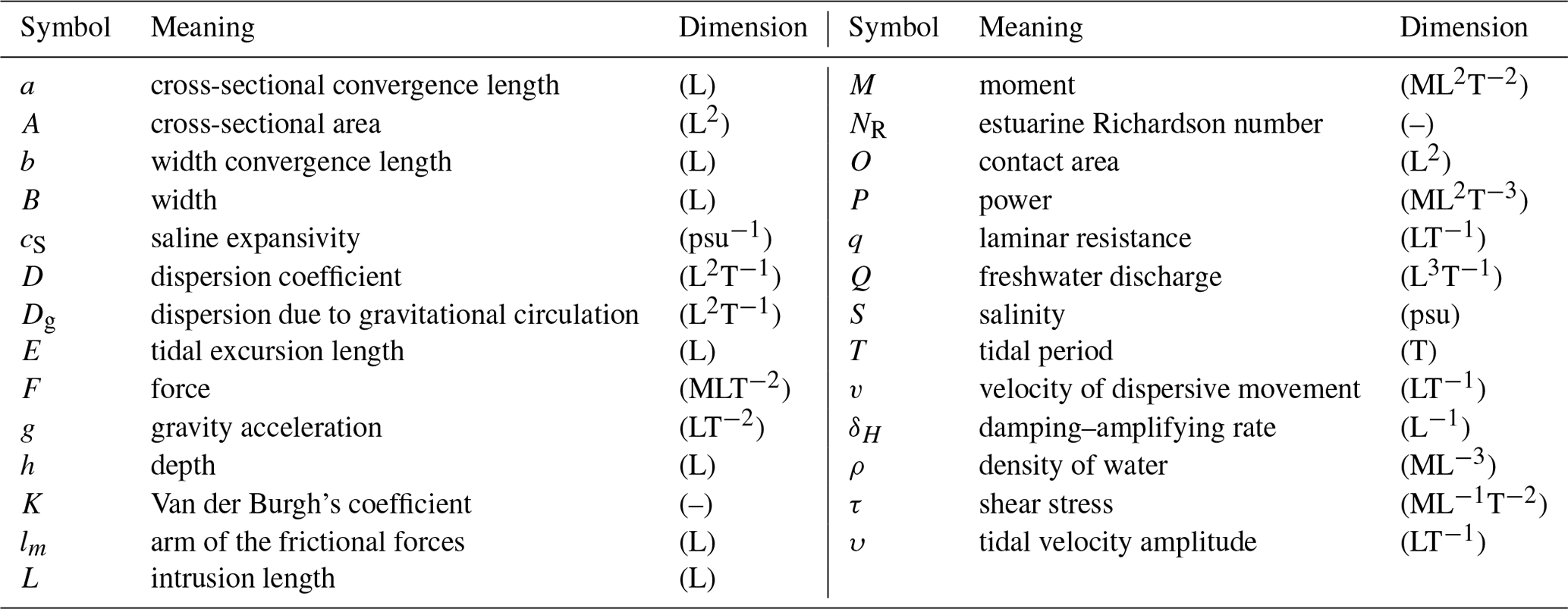
- Appendix A: Notation
- Appendix B: Application of the maximum power method
- Author contributions
- Competing interests
- Special issue statement
- Acknowledgements
- Review statement
- References
- Abstract
- Introduction
- Moment balance for an open estuary system
- Empirical validation and discussion
- Combination of the MP and VDB methods
- Conclusions
- Data availability
- Appendix A: Notation
- Appendix B: Application of the maximum power method
- Author contributions
- Competing interests
- Special issue statement
- Acknowledgements
- Review statement
- References