Arctic amplification under global warming of 1.5 and 2 °C in NorESM1-Happi

Differences between a 1.5 and 2.0 ^∘C warmer climate than 1850 pre-industrial conditions are investigated using a suite of uncoupled (Atmospheric Model Intercomparison Project; AMIP), fully coupled, and slab-ocean experiments performed with Norwegian Earth System Model (NorESM1)-Happi, an upgraded version of NorESM1-M. The data from the AMIP-type runs with prescribed sea-surface temperatures (SSTs) and sea ice were provided to a model intercomparison project (HAPPI – Half a degree Additional warming, Prognosis and Projected Impacts; http://www.happimip.org/, last access date: 14 September 2019). This paper compares the AMIP results to those from the fully coupled version and the slab-ocean version of the model (NorESM1-HappiSO) in which SST and sea ice are allowed to respond to the warming, focusing on Arctic amplification of the global change signal.

The fully coupled and the slab-ocean runs generally show stronger responses than the AMIP runs in the warmer worlds. The Arctic polar amplification factor is stronger in the fully coupled and slab-ocean runs than in the AMIP runs, both in the 1.5 ^∘C warming run and with the additional 0.5 ^∘C warming. The low-level Equator-to-pole temperature gradient consistently weakens more between the present-day climate and the 1.5 ^∘C warmer climate in the experiments with an active ocean component. The magnitude of the upper-level Equator-to-pole temperature gradient increases in a warmer climate but is not systematically larger in the experiments with an active ocean component. Implications for storm tracks and blocking are investigated. We find considerable reductions in the Arctic sea-ice cover in the slab-ocean model runs; while ice-free summers are rare under 1.5 ^∘C warming, they occur 18 % of the time in the 2.0 ^∘C warming simulation. The fully coupled model does not, however, reach ice-free conditions as it is too cold and has too much ice in the present-day climate.

Differences between the experiments with active ocean and sea-ice models and those with prescribed SSTs and sea ice can be partially due to ocean and sea-ice feedbacks that are neglected in the latter case but can also in part be due to differences in the experimental setup.

1 Introduction

In the Paris Agreement, the parties of the United Nations Framework Convention on Climate Change (UNFCCC) established a long-term temperature goal for climate protection of “holding the increase in the global average temperature to well below 2 ^∘C above pre-industrial levels and pursuing efforts to limit the temperature increase to 1.5 ^∘C above pre-industrial levels, recognizing that this would significantly reduce the risks and impacts of climate change” (UNFCCC, 2015). This has triggered considerable attention from climate modelling groups and researchers alike (e.g. Hulme, 2016; Peters, 2016; Rogelj and Knutti, 2016; Mitchell et al., 2016; Anderson and Nevins, 2016; Boucher et al., 2016; Schleussner et al., 2016; and the special issue of the electronic journal Earth System Dynamics: https://www.earth-syst-dynam.net/special_issue909.html, last access: 14 September 2019). The Special Report from the Intergovernmental Panel on Climate Change (IPCC) was published in October 2018 (http://www.ipcc.ch/report/sr15/, last access: 14 September 2019).

In addressing differences in the climate impacts of the 1.5 and 2 ^∘C global warming targets (we use the word “targets”, although “upper bounds” would be more correct), there are two basic weaknesses of the available climate projections from the Coupled Model Intercomparison Project (CMIP) as reported in the assessment reports from the Intergovernmental Panel on Climate Change (IPCC). There is a small body of research assessing impacts of 1.5 ^∘C warming compared to that for higher emission scenarios (James et al., 2017). The CMIP simulations are moreover generally designed on the basis of development scenarios that give rise to certain top-of-the-model-atmosphere (TOA) radiative forcings, rather than selected temperature targets. Because different models simulate different responses of global near-surface temperature to a given TOA radiative forcing, new types of model simulations are necessary to provide a scientifically based evaluation of climate statistics for specific temperature targets.

Under the acronym HAPPI (Half a degree Additional warming, Prognosis and Projected Impacts; http://www.happimip.org/, last access: 14 September 2019), Mitchell et al. (2017) provided an experimental framework for model simulations of the present-day (PD) climate and climates that are 1.5 and 2.0 ^∘C warmer than the pre-industrial. The experiments are similar to those under the Atmospheric Model Intercomparison Project (AMIP) protocol, employing active atmosphere and land components from state-of-the-art coupled Earth system models (ESMs) and prescribed sea-surface temperatures (SSTs) and sea ice. A multi-model ensemble with several hundred members was produced, enabling robust statistics for flow changes and rare events (e.g. Baker et al., 2018; Barcikowska et al., 2018; Li et al., 2018; Liu et al., 2018; Senerivatne et al., 2018; Wehner et al., 2018).

Warming of 1.5 and 2.0 ^∘C has also been investigated in fully coupled models. Sanderson et al. (2017) developed and applied an emulator to arrive at forcing scenarios that would produce global warming of 1.5 and 2 ^∘C above pre-industrial levels in the Community Earth System Model version 1 (CESM1; Hurrell et al., 2013). Sigmond et al. (2018) created scenarios by first running the Representative Concentration Pathway (RCP) scenario corresponding to an increased radiative forcing of 8.5 W m⁻² by the end of the 21st century (RCP8.5; van Vuuren et al., 2011) and then branching off the 1.5 and 2.0 ^∘C warming experiment when the near-surface temperature warming was 1.5 and 2.0 ^∘C relative to pre-industrial conditions, setting the emissions of anthropogenic CO₂ and aerosols to zero in the Canadian Earth System Model version 2 (CanESM2). Both Sanderson et al. (2017) and Sigmond et al. (2018) carried out century-scale ensemble simulations. One striking result from these studies is the strong increase in the probability of having an ice-free Arctic Ocean in the summer with the additional 0.5 ^∘C warming (the difference between the 1.5 and 2 ^∘C warming scenarios). This aspect of the response to the 1.5 and 2.0 ^∘C warming is not evident in the HAPPI experiments because the sea ice is prescribed but will be further addressed in the present paper.

We use various configurations of the Norwegian Earth System Model, NorESM1-Happi, which is an upgraded version of NorESM1-M used in CMIP5 (Bentsen et al., 2013; Iversen et al., 2013; Kirkevåg et al., 2013). The upgrades include double horizontal resolution and improved treatment of sea ice. The model was previously run in AMIP mode (NorESM1-HappiAMIP) to contribute a large ensemble of simulations to HAPPI. In order to study the role of the ocean and sea ice, here we provide fully coupled simulations targeting quasi-sustained global warming levels of 1.5 and 2 ^∘C above pre-industrial levels. The forcings are constructed on the basis of those from the RCPs corresponding to an increased radiative forcing of 2.6 and 4.5 W m⁻² by the end of the 21st century (RCP2.6 and RCP4.5) but with important changes to the time evolution of the CO₂ concentrations. We also use a configuration where the full ocean model is replaced by a thermodynamic slab-ocean (SO) model (NorESM1-HappiSO). This configuration is an intermediate option between the fully coupled and the AMIP configurations, applied in order to partly correct for temperature biases in the fully coupled simulations but still allowing for SST and sea-ice feedbacks.

The role of Arctic amplification for specific warming levels (Arrhenius, 1896; Manabe and Stouffer, 1980; Holland and Bitz, 2003; Feldl et al., 2017) is relevant for the consequences of the Paris Agreement. This is primarily due to the associated in situ changes in the sea-ice and snow cover but also due to the potential triggering of irreversible feedbacks. Other important feedbacks include changes in midlatitude weather patterns and variability (Francis and Vavrus, 2012; Screen and Simmonds, 2013; Cohen et al., 2014; Screen, 2014, 2017a, b; Barnes and Polvani, 2015; Screen and Francis, 2016; Vihma, 2017; Screen et al., 2018; Coumou et al., 2018).

Arctic amplification is predominantly driven by a positive regional lapse-rate feedback (negative at lower latitudes) in winter and a positive albedo feedback in summer (Winton, 2006; Pithan and Mauritsen, 2014). While the amplitude and pattern of Arctic amplification varies between models, it is nevertheless a robust response to global warming. Even the remotely localized forcing caused by reduced European sulfate aerosols since the 1980s has produced maximum warming in the Arctic (Acosta Navarro et al., 2016). Under the CMIP6 protocol, a Polar Amplification Model Intercomparison Project (PAMIP) is endorsed (Smith et al., 2019).

In this paper, we focus on the Northern Hemisphere (NH) climate response to global warming of 1.5 and 2 ^∘C above pre-industrial levels in NorESM, and on how the response differs depending on whether the model is run with fixed SSTs and sea ice (as in HAPPI) or with active ocean and sea-ice models. We study changes in Arctic amplification, Arctic sea ice, meridional temperature contrasts for different heights, and the storm tracks. We also consider blocking, although its representation in rather coarse-resolution climate models is known to be of mixed quality (Dawson et al., 2012; Davini and D'Andrea, 2016; Woolings et al., 2018).

Section 2 provides an overview of NorESM1-Happi and its SO version NorESM1-HappiSO, along with a summary of the differences between NorESM1-Happi and its predecessor NorESM1-M. The 1.5 and 2.0 ^∘C warming scenarios are described in Sect. 3. Results are presented in Sects. 4–7. A summary and discussion are given at the end in Sect. 8. The Supplement to the paper contains an extensive validation of NorESM1-Happi in line with the CMIP5 protocol.

2 The model

In this section, we give a brief overview of the fully coupled NorESM1-Happi model, which is an upgraded version of NorESM1-M used for CMIP5. A more exhaustive overview of NorESM1-M is given in Bentsen et al. (2013), Iversen et al. (2013), and Kirkevåg et al. (2013).

NorESM1-M is based on the fourth version of the Community Climate System Model (CCSM4) developed in the Community Earth System Model project at the US National Center for Atmospheric Research (NCAR) in collaboration with many partners (Gent et al., 2011).

The atmosphere component of NorESM1-M and NorESM1-Happi is the “Oslo” version of the CCSM4's Community Atmosphere Model version 4 (CAM4-Oslo). It is based on the CAM4 (Neale et al., 2010, 2013) but is extended with an online aerosol module for aerosol life-cycle calculations and aerosol–cloud–radiation interactions (Kirkevåg et al., 2013).

The ocean component is an elaborated version of the Miami Isopycnic Community Ocean Model (MICOM). This is an entirely different ocean component than the one used in CCSM4. The MICOM version used in NorESM1-M and -Happi has been adapted for multi-century simulations in coupled mode (Assmann et al., 2010; Otterå et al., 2010) and includes several extensions compared to the original MICOM (Bentsen et al., 2013).

The land and sea-ice components and the coupler are the same as in the CCSM4. The land component is the fourth version of the Community Land Model (CLM4; Oleson et al., 2010; Lawrence et al., 2011), including the SNow, ICe, and Aerosol Radiative model (SNICAR; Flanner and Zender, 2006). The sea-ice component is the fourth version of the Los Alamos Sea Ice Model (CICE4; Gent et al., 2011; Holland et al., 2012). The coupler is the version 7 coupler (CPL7; Craig et al., 2012).

The ocean and sea-ice components of NorESM1-M and NorESM1-Happi were run with the standard CCSM4 land mask and ocean grid (the gx1v6) with 1.125^∘ resolution along the Equator and with the NH grid singularity located over Greenland. The atmosphere component, CAM4-Oslo, was run with a horizontal resolution of 0.95^∘ latitude by 1.25^∘ longitude (in short: 1^∘ resolution) in NorESM1-Happi and the double of the mesh width (2^∘ resolution) in NorESM1-M. In both versions, CAM4-Oslo has 26 hybrid sigma-pressure levels in the vertical and a model top at 2.194 hPa. The land component (CLM4) employs the same horizontal grid as CAM4-Oslo, except for the river transport model which is configured on its own grid with a horizontal resolution of 0.5^∘ in both model versions.

Differences between NorESM1-Happi and NorESM1-M include finer horizontal resolution in the atmosphere and land, as described above, but also a few upgrades in the ocean, sea ice, and atmosphere components. In NorESM1-Happi, inertia–gravity waves are damped in shallow ocean regions in order to remove spurious oceanic variability in high-latitude shelf regions (Seland and Debernard, 2014). The albedo of wet snow on sea ice is reduced by increasing the assumed wet snow grain size and by allowing a more rapid metamorphosis from dry to wet snow. This affects the Arctic sea ice more than the Antarctic sea ice, since the latter is less frequently influenced by mild and humid air (Seland and Debernard, 2014).

In the atmosphere, an error in the aerosol life-cycle scheme (Kirkevåg et al., 2013) was found and rectified, resulting in faster condensation of secondary gas-phase matter on pre-existing particles. The changes in atmospheric residence time of aerosols compared to NorESM1-M are minor, except for the reductions for black carbon (BC) and organic matter due to more efficient wet deposition. This mainly affects the upper-air BC concentrations (Fig. S1 in the Supplement). Samset et al. (2013) and Allen and Landuyt (2014) indicated that NorESM1-M has too-high upper-air concentrations of BC aerosols. This could cause overestimated absorption of solar radiation, suppressed upper-level cloudiness, and exaggerated static stability but has minor impacts on surface temperatures, surface energy fluxes, and multi-decadal variability associated with the deep oceans (Sand et al., 2015; Stjern et al., 2017). To the extent that the observations from the HIPPO campaign (Schwarz et al., 2013) are representative for the vertical distribution of BC in general, NorESM1-Happi still mixes the BC too high up in the troposphere. A comprehensive discussion of the aerosols in a recently updated NorESM version (NorESM1.2) is given in Kirkevåg et al. (2018).

2.1 Emulating the oceanic response with a slab-ocean model

NorESM1-HappiSO, the SO (slab-ocean) model version of NorESM1-Happi, has the same atmosphere, land and sea-ice components, and coupler as the fully coupled model. The ocean component is, however, replaced by a SO model, which is a simplified two-dimensional ocean model that represents a well-mixed layer immediately below the ocean surface.

A SO model does not calculate the ocean circulation and associated fluxes but treats the upper-ocean mixed layer as a single layer which buffers heat fluxes through the ocean surface, that is, a thermodynamic “slab” governed by the equation

$$\begin{array}{}\text{(1)}& {\mathit{\rho }}_{\mathrm{0}}{c}_{\mathrm{0}}{h}_{\mathrm{mix}}{\displaystyle \frac{\partial T_{\mathrm{mix}}}{\partial t}}=F_{\mathrm{net}}-Q_{\mathrm{f}}-\mathit{\alpha }{\mathit{\rho }}_{\mathrm{0}}{c}_{\mathrm{0}}{h}_{\mathrm{mix}}\left(T_{\mathrm{mix}}-T_{\mathrm{mixExt}}\right)/\mathit{\tau },\end{array}$$

where h_mix is the thickness of the slab which varies in space but not in time, ρ₀ and c₀ are the density and specific heat capacity of the seawater, T_mix is the mixed-layer temperature, F_net is the net input of heat through the ocean surface from the atmosphere and sea ice, and Q_f is the net divergence of heat not accounted for by the explicit processes which are needed to maintain a stable climate with a predefined geographical distribution of SST. The last term on the right-hand side is a restoring term that can, depending on the value of α, be used to relax the T_mix field toward an externally imposed temperature field T_mixExt when estimating Q_f. τ is the prescribed timescale for the adjustment. For free SO runs, α=0.

The realism of the SO model climate depends on how Q_f is prescribed. In Bitz et al. (2012), Q_f is calculated using h_mix, T_mix, and F_net from a fully coupled stable control simulation, setting α=0. Both h_mix and T_mix should represent an assumed well-mixed layer in the vertical. With an annual mean (but still spatially variable) mixed-layer thickness, it is quite straightforward to obtain balance with the annual cycle of heat (Bitz et al., 2012). This method gives a mean SST distribution from the SO model which is very similar to, and consistent with, the climate of the fully coupled model when the external forcing is unchanged. Here, this method has been used when estimating the equilibrium climate sensitivity (ECS) for runs with abrupt CO₂ doubling (ΔT_eq2=3.31 ^∘C) and CO₂ quadrupling (ΔT_eq4=6.74 ^∘C), giving a global-mean change in the equilibrium near-surface temperature (ΔT_eq) of 3.34 ^∘C (the average of ΔT_eq2 and ΔT_eq4∕2) for doubling of the atmospheric CO₂ concentrations (Table S7). The Q_f used in these experiments was diagnosed from the 1850 fully coupled piControl experiment with NorESM1-Happi (Sect. 2.2) and kept constant in the different SO runs.

Here, the primary purpose of running NorESM1-HappiSO is to carry out simulations that are similar to the AMIP simulations performed for the HAPPI project but where the sea ice is free to respond to the imposed warming. One drawback with the method of Bitz et al. (2012) for quantifying Q_f is that biases in SST and the mean climate from the fully coupled model are reflected in the SO model. This makes comparison with the AMIP experiments, where the PD SSTs and sea-ice cover are determined from observations, difficult. Therefore, as an alternative, we use a restoring method similar to Williams et al. (2001) and Knutson (2003), where a separate calibration run of the SO model is done by setting α=1 in Eq. (1). The externally imposed temperature field, T_mixExt, is valid for some specific period and can be based on observations or model output. After this run, the new Q_f is defined by adding the monthly climatology of the restoring flux to the Q_f used in the calibration run. Then, when used in a free SO run (setting α=0), the new Q_f ensures a modelled T_mix climate which is close to the T_mixExt field imposed during the calibration. Note that in the versions of NorESM considered here, the mixed layer temperature T_mix is equivalent to the SST field. Therefore, we can use observed SST as the imposed external field during the calibration phase.

We have kept the sea-ice model free of any restoring or constraints to observed fields during the calibration. This increases the realism of the ice–ocean heat fluxes going into F_net and ensures consistent changes in sea-ice mass and energy. As in Bitz et al. (2012), the sea ice in the SO setup employs the full CICE4 dynamic and thermodynamic model, which is the same as that used in the fully coupled NorESM1-M and NorESM1-Happi models. However, some tuning of snow albedo over sea ice has been done to increase the realism of sea-ice extent under PD conditions when using the restoring method for specifying Q_f. See Sect. 3.3 for more details on the experimental setup.

2.2 Qualifying NorESM1-Happi: CMIP5 experiments

We performed a full range of CMIP5 experiments with the fully coupled NorESM1-Happi model to document the performance of the model, and to obtain valid historical and RCP8.5 runs for the fully coupled PD experiment (Sect. 3.2). The CMIP5 experiments are summarized in Table 1. The setup of the simulations follows that of the original CMIP5 simulations with NorESM1-M (Bentsen et al., 2013; Iversen et al., 2013; Kirkevåg et al., 2013).

Table 1 Overview of the NorESM1-X versions referred to in this paper.

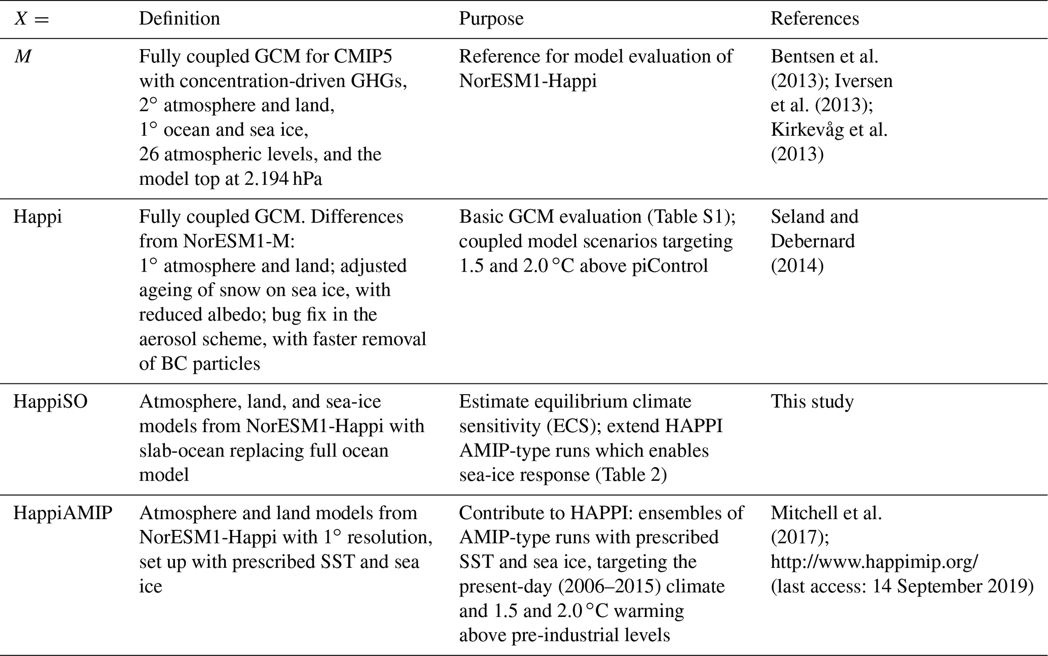
NorESM1-Happi with 1^∘ resolution was spun up for 1850 conditions over 300 years, starting from model year 600 of the NorESM1-M spin-up with 2^∘ resolution over atmosphere and land. The ocean and sea ice were in both cases run with 1^∘ resolution. The pre-industrial control experiment (piControl) was started from the end of the spin-up, in model year 900. The three historical experiments were started from the piControl in model years 930 (Hist1), 960 (Hist2), and 990 (Hist3), that is, from three representations of the climate state in the year 1850. The three RCP8.5 experiments were started from the three historical experiments in the year 2006. The code upgrades were introduced during the spin-up period, while the bug fix in the aerosol scheme was introduced at the beginning of the piControl experiment, causing some adjustments over the first few years.

Here, we briefly summarize the extensive model validation of NorESM1-Happi against NorESM1-M, observations, and reanalysis given by Tables S1–S7 and Figs. S1–S15 in the Supplement. The piControl simulation for NorESM1-Happi is considerably more stable than that for NorESM1-M, mainly because the control run started from a state closer to equilibrium. The NorESM1-Happi piControl experiment also deviates less from the World Ocean Atlas of 2009 (Locarnini et al., 2010; Antonov et al., 2010) than NorESM1-M. The increased horizontal resolution results in reduced cloudiness in NorESM1-Happi (compared to NorESM1-M), and along with this a cold bias, a faster atmospheric cycling of freshwater, and overestimated precipitation globally (Table S4 and Fig. S5). The atmospheric residence time and ocean-to-continent transport of water vapour appears satisfactory (Table S6). Also, the thermohaline forcing of the Atlantic meridional overturning circulation (AMOC) has strengthened and is probably too strong (Fig. S14).

NorESM1-Happi has a better representation of sea ice (Table S5 and Fig. S4), improved NH extratropical cyclone activity (Fig. S11) and blocking activity (Fig. S12), and a fair representation of the Madden–Julian oscillation (Fig. S10). The amplitude of the El Niño–Southern Oscillation (ENSO) signals is reduced and is too small, although the frequency is improved (Fig. S13). NorESM1-Happi has lower climate sensitivity (3.34 ^∘C at CO₂ doubling) than NorESM1-M (3.50 ^∘C) and slightly higher climate sensitivity than CCSM4 (3.20 ^∘C; Table S7). The lapse-rate, albedo, and to a smaller extent the short-wave water vapour feedbacks contribute to Arctic amplification in both model versions (Fig. S15).

3 The 1.5 and 2.0 ^∘C warming scenarios

3.1 The AMIP experiments

The “AMIP experiments” are those performed with NorESM1-Happi for the model intercomparison project HAPPI. The target of the experiments is to investigate the regional impacts of global warming under stabilization scenarios that are 1.5 and 2.0 ^∘C warmer than the 1850 climate. The three large ensemble experiments are the PD climate (for the years 2006–2015), a climate that is 1.5 ^∘C warmer than the pre-industrial (1850) climate, and a climate that is 2.0 ^∘C warmer. We refer to these as the AMIP-PD, the AMIP-15, and the AMIP-20 experiments, respectively.

Designing a coupled model experimental protocol for 1.5 and 2.0 ^∘C warming targets requires determining forcing conditions that will produce the target global-mean temperature change and other characteristics of the warmer climate state. The same forcing conditions may, however, produce different temperature responses in different models. The CMIP5 models, for instance, display considerable spread in the near-surface temperature response for RCP2.6. While the multi-model mean response is very close to 2.0 ^∘C, the spread across the 95 %–5 % range is approximately 1.5 ^∘C (see Fig. 2 in Mitchell et al., 2017). Fully coupled models are moreover computationally expensive because they require centuries or longer to approach new equilibria after sustained shifts in the TOA radiation balance.

The experiments in the HAPPI project were therefore run with prescribed SSTs and sea ice. This constrains the climate state and makes it computationally feasible to run large ensembles. The experimental setup resembles the AMIP protocol; thus, we refer to the version of NorESM1-Happi that follows the HAPPI protocol as NorESM1-HappiAMIP.

The construction of the input data for the HAPPI experiments is described in detail by Mitchell et al. (2017). The main points are listed below:

• In the AMIP-PD experiment, the SST and sea-ice fields are based on observations (Taylor et al., 2012). Anthropogenic greenhouse gas (GHG) concentrations (including CO₂, CH₄, N₂O, and chlorofluorocarbons; CFCs), emissions of aerosols and their precursors, ozone concentrations, and land-use changes are taken from RCP8.5 for the years 2006–2015, as it is common procedure to use RCP8.5 to extend the historical period beyond 2005 (van Vuuren et al., 2011).

• In the AMIP-15 experiment, anthropogenic GHG and ozone concentrations, land-use, and aerosol data are taken from RCP2.6 for the year 2095. The SST increase relative to PD is the CMIP5 multi-model mean difference between the years 2091–2100 from RCP2.6 and 2006–2015 from RCP8.5. Natural forcings are as for AMIP-PD. Sea-ice concentrations are estimated from a linear regression between observed anomalies of SST and sea ice (see Mitchell et al., 2017, p. 575, for details).

• In the AMIP-20 experiment, the SST and sea-ice concentration differences are derived in a similar way but using a weighted mean between RCP2.6 and RCP4.5 (0.41 for RCP2.6 and 0.59 for RCP4.5). The same weights are used for CO₂ (assuming a logarithmic relation). All other forcings are as for AMIP-15.

The HAPPI experimental protocol does not cover sea-ice thickness. As is standard in NorESM, the sea-ice thickness is held fixed at 2 m in the NH and 1 m in the Southern Hemisphere (SH).

The NorESM1-HappiAMIP data set includes 125 ensemble members for each experiment, each of length 10 years (after a 1-year spin-up which is discarded from the analysis), giving 3750 years of data. To allow for dynamical downscaling, high-temporal-resolution output from 25 members of each experiment was stored. The data are available for download at http://portal.nersc.gov/c20c/data.html (last access: 14 September 2019).

3.2 The fully coupled (CPL) experiments

One shortcoming of the AMIP-type simulations is that while they calculate the effects of prescribed changes in the ocean and sea ice on the atmosphere, they cannot calculate how these atmospheric changes may feed back on the ocean and sea ice. To investigate the effects of having ocean and sea-ice components that are free to respond to changes and variability in other parts of the climate system, we have conducted fully coupled experiments with NorESM1-Happi that target 1.5 and 2.0 ^∘C warming compared to pre-industrial temperature levels (CPL-15 and CPL-20). The forcing data in these experiments are based on RCP2.6 and RCP4.5. The emissions of anthropogenic aerosols and aerosol precursors, land-use changes, and concentrations of GHGs apart from CO₂ follow those in RCP2.6. Thus, we have chosen to mimic the evolution towards the two temperature targets by manipulating the prescribed time evolution of the CO₂ concentration (Fig. 1).

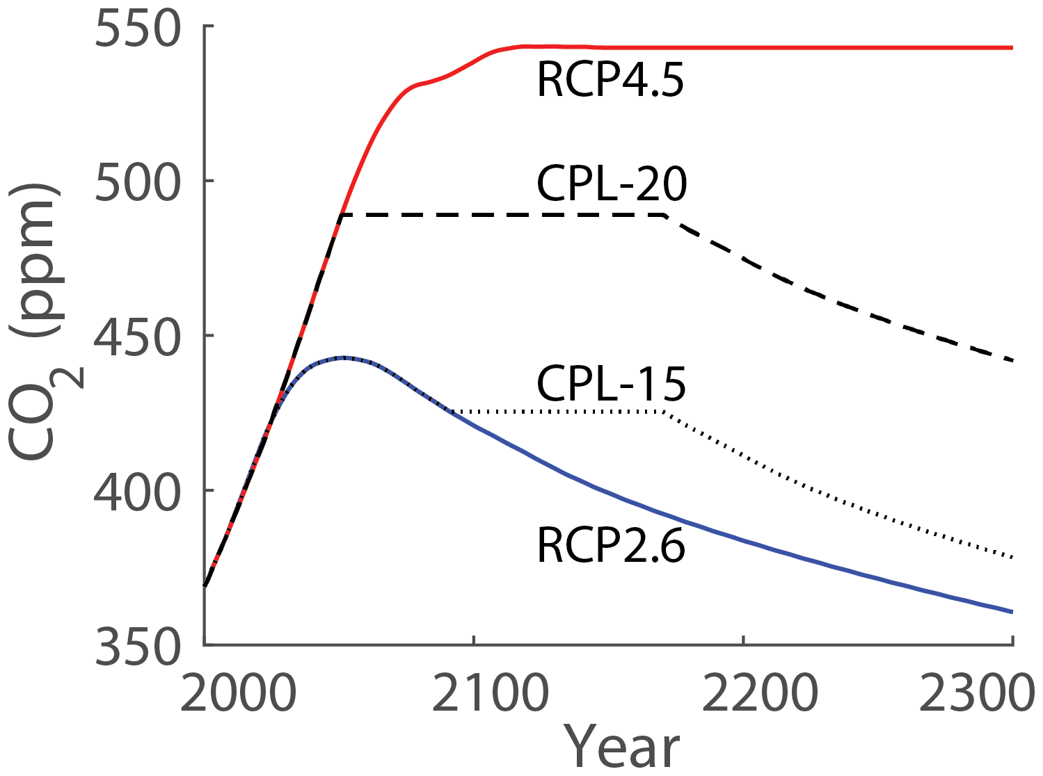
Figure 1 Time evolution of prescribed atmospheric CO₂ concentration for the 1.5 and 2.0 ^∘C warming experiments with NorESM1-Happi. The 1.5 ^∘C experiment (dotted black line) initially follows RCP2.6 (solid blue line). At year 2095, the concentration deviates from RCP2.6, staying constant until year 2170, and decreases thereafter. The 2.0 ^∘C experiment (dashed black line) similarly follows RCP4.5 (solid red line) at first but branches off at year 2050. The concentration is then constant until the year 2170 before decreasing in the same fashion as in the 1.5 ^∘C experiment. Units are in ppm.

It should be made clear that other temperature evolutions are possible by alternative combinations of forcing data, but an adequate discussion of this is far beyond the scope of the present paper. Furthermore, it is impossible in practice to constrain atmospheric concentrations directly. Atmospheric concentration levels result from the combination of emissions and removal processes, some of which are controllable in practice. We emphasize that because the CO₂ in NorESM1-Happi is concentration-driven, and not emission-driven as in Sigmond et al. (2018), switching off the anthropogenic CO₂ emissions to create stabilized scenarios with this model is impossible.

The constructed scenarios were inspired by those in HAPPI, with the CPL-15 being based on RCP2.6 and CPL-20 being based on a combination of RCP2.6 and RCP4.5. The details of the scenarios were determined through an iterative trial-and-error process. Although also inspired by the much more sophisticated method by Sanderson et al. (2017), we simply ran the model for 1–2 centuries based on a few constructed time profiles of CO₂ concentrations. The results in this paper are taken from the version that was most successful in hitting the two temperature targets.

In CPL-15, the CO₂ concentration follows RCP2.6 from the year 2000 to the year 2095, after which it stays constant until the year 2170 and then decreases following the pattern assumed in the original RCP2.6 from the year 2095 onwards. Thus, the decrease is delayed 75 years compared to RCP2.6. In CPL-20, the CO₂ concentration follows RCP4.5 from the year 2000 to the year 2050, then stays constant until the year 2170, after which it decays in the same fashion as CPL-15 but starts from the higher concentration level.

The fully coupled PD (CPL-PD) climate is represented by the 30-year time period 1991–2020 using output from CMIP5 experiments carried out with NorESM1-Happi. We use the period (1991–2005) from three individual simulations of the historical climate (Hist1, Hist2, and Hist3; see Sect. 2.2 or Table S1) and extend them with the years 2006–2020 from three individual simulations of RCP8.5 (Sect. 2.2). Thus, CPL-PD, CPL-15, and CPL-20 are all sampled by 90 years of simulations with the fully coupled NorESM1-Happi model.

The scenario runs CPL-15 and CPL-20 both start from simulation year 2005 of the Hist1 experiment. Figure 2 shows the change in near-surface temperature for Hist1 (1850–2005) and for the CPL-15 and CPL-20 experiments (2006–2230) relative to the pre-industrial climate calculated under constant driving conditions valid for the year 1850 (the piControl experiment; see Sect. 2.2 or Table S1). The global-mean temperature warms rapidly between the years 1960 and 2050; then, the response flattens out over the next 150 years. In what follows, we study results from the 90-year period (2111–2200) for which the mean temperature increase in CPL-15 and CPL-20 is 1.51 and 1.97 ^∘C relative to pre-industrial conditions and 0.69 and 1.15 ^∘C relative to CPL-PD (see discussion of Table 3 in Sect. 4.1).

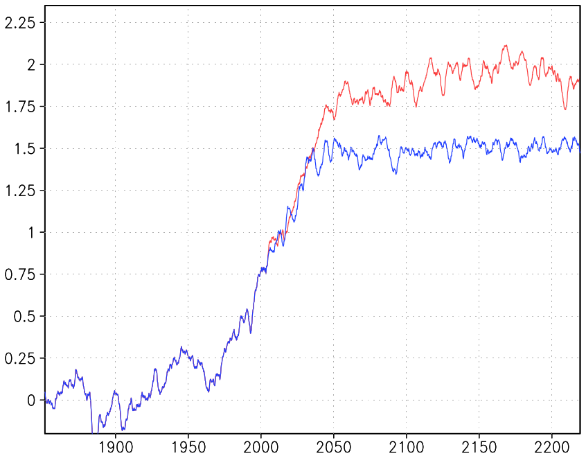
Figure 2 Time evolution of the global-mean near-surface temperature response in the Hist1 experiment (1850–2005; blue) and the CPL-15 (2006–2230; blue) and the CPL-20 experiments (2006–2230; red) relative to pre-industrial conditions (years 1850–1852). A 3-year running average is used for both curves. Units are in degrees Celsius.

The experiments are, however, not entirely stabilized. By the end of the 22nd century, both CPL-15 and CPL-20 still have a positive radiative imbalance at the top of the model atmosphere (around 0.7 W m⁻², not shown) and a positive heat flux into the ocean at depths below 200 m (Fig. 3). The net heat uptake in the upper ocean is, however, small at that point. The AMOC decreases with time over the first 100 years and is relatively stable over the last 150 years (Fig. 4).

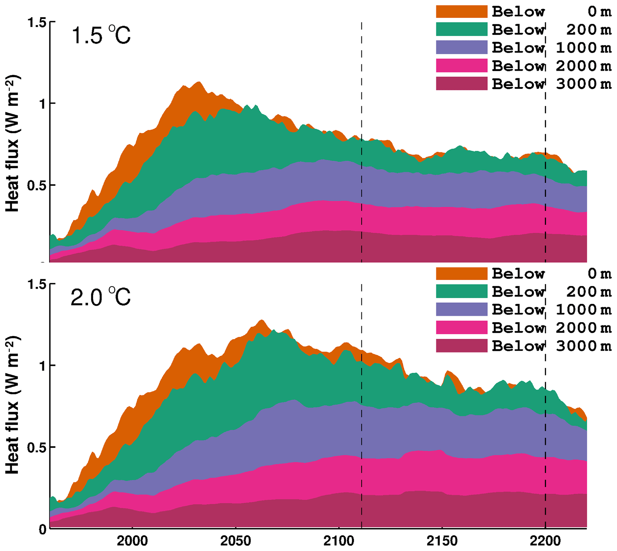
Figure 3 Ocean heat uptake as a function of time in the CPL-15 (a) and CPL-20 (b) experiments. Shown is the heat uptake for depths 0–200 m (orange shading), 200–1000 m (green shading), 1000–2000 m (blue shading), 2000–3000 (pink shading), and below 3000 m (dark pink shading). Dashed vertical lines emphasize the time period analysed in this study. Units are in W m⁻².

Figure 4 Time evolution of the maximum in the AMOC (Atlantic meridional overturning circulation) at 26.5^∘ N in Hist1, RCP2.6 (black) and in the 1.5 ^∘C (red) and 2.0 ^∘C (blue) warming experiments with NorESM1-Happi. A 10-year running average is used for all curves. Units are in Sv.

Our fully coupled experiments differ from those in Sanderson et al. (2017) and in Sigmond et al. (2018). Sanderson et al. first used a climate emulator to construct concentration scenarios and then used these scenarios to produce stabilized 1.5 and 2.0 ^∘C warming experiments with the CESM1. Sigmond et al. (2018) branched the warming experiments off from RCP8.5, setting the emissions of anthropogenic CO₂ and aerosols to zero in the CanESM2. The simulations presented in this study are far from reaching equilibrated climate states but are quasi-stable over 90-year periods after a spin-up of 100 years from PD. Full equilibration over several centuries is likely to produce different climate states (Gillet et al., 2011).

3.3 The slab-ocean experiments

While results from the coupled simulations above will help us understand how 1.5 and 2.0 ^∘C warming might manifest in the fully coupled Earth system, CPL-15 and CPL-20 are not stabilized scenarios like the AMIP experiments. Moreover, Fig. 5 shows that the fully coupled PD experiments (Fig. 5a, d, g, and j) exhibit larger biases than the AMIP experiments (Fig. 5c, f, i, and l) relative to ERA-Interim (Dee et al., 2011) in all seasons. Prescribing the SSTs and sea ice to observationally based fields constrains the climate in the AMIP-PD experiments, yielding smaller biases in the simulated climate. To be able to examine 1.5 and 2.0 ^∘C warming experiments in a model which has smaller biases, but where the sea ice and SSTs are also free to respond, we have designed a SO configuration of NorESM1-Happi, NorESM1-HappiSO (see Sect. 2.1 for details).

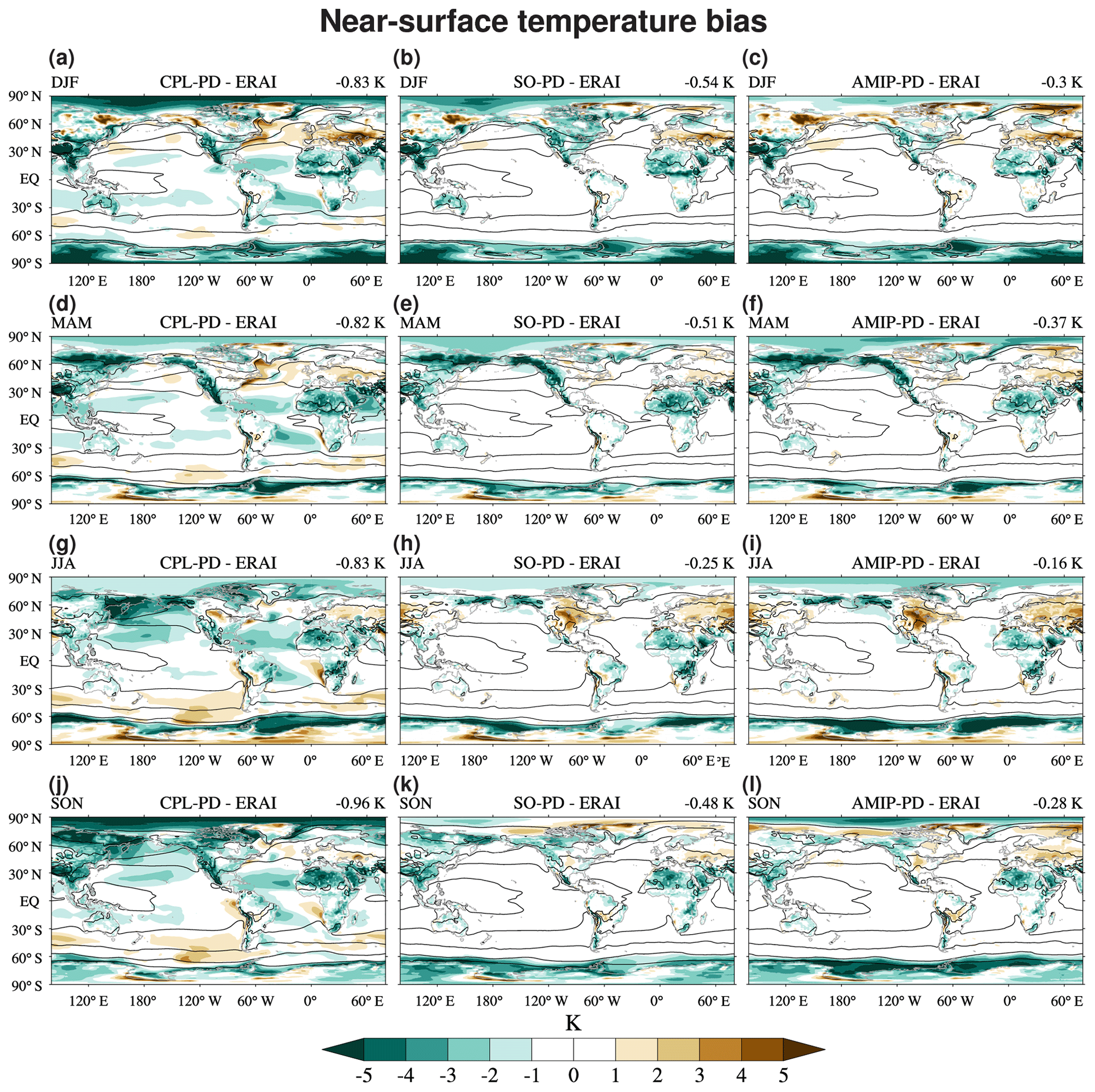
Figure 5 Near-surface temperature bias relative to ERA-Interim (colours) and near-surface temperature climatology (black contours; 260 to 350 K in increments of 10 K) for PD experiments from NorESM1-Happi (a, d, g, j), NorESM1-HappiSO (b, e, h, k), and NorESM1-HappiAMIP (c, f, i, l). We use the years 1986–2015 from ERA-Interim. The time periods for the NorESM experiments are the default periods given in Sect. 3. The global-mean ensemble-mean bias is given in the upper-right corner of each panel. Units are in Kelvin (a–l).

We have conducted free-running SO experiments for the PD climate (SO-PD) and for climates that are 1.5 and 2.0 ^∘C warmer than the pre-industrial (SO-15 and SO-20). The SO model has been calibrated to mimic the three HAPPI experiments (AMIP-PD, AMIP-15, and AMIP-20), using the same forcings for GHGs, aerosols, ozone, and land use. In SO-PD, the SSTs are constrained to stay close to the observed values from AMIP-PD. The SST differences for SO-15 and SO-20 are based on the SST response in CPL-15 and CPL-20 relative to CPL-PD for consistency with the model climate in NorESM1-Happi. This is in line with the recommendations of Bitz et al. (2012) when the sea-ice model is the same as in the fully coupled model version. An overview of the experiments is provided in Table 2.

Table 2 Overview of the NorESM1-HappiSO experiments and their calibration. Q_f is the net divergence of heat not accounted for by the explicit processes, which is needed to maintain a stable climate with a predefined geographical distribution of SST. In SO-PD, SO-15, and SO-20, a restoring term $-(T_{\mathrm{mix}}-T_{\mathrm{mixExt}})/\mathit{\tau }$ is included in Q_f, where τ=30 d is the applied timescale of adjustment. Notice that sea ice is not restored except for via the indirect effect of the SST restoring term.

In the present case, the purpose of the SO model is to emulate regional patterns of the climate response given a targeted global near-surface temperature change relative to the pre-industrial climate, considering the observed and analysed climate at PD (2006–2015). The experiments with NorESM1-HappiSO are designed to be comparable to the NorESM1-HappiAMIP experiments, in which the SST and sea ice are prescribed (Sect. 3.1). Three different calibrations of Q_f (Eq. 1) are therefore performed using the restoring method (Sect. 2.1). For SO-PD, we use 12-year averaged SSTs determined by the observationally based Operational Sea Surface Temperature and Sea Ice Analysis (OSTIA) for the years 2005–2016 (Donlon et al., 2012). In practice, this calibration also reduces biases. For SO-15 and SO-20, we determine new Q_f fields that adjust the model to SST fields which are consistent with 1.5 and 2.0 ^∘C warming. To obtain these fluxes, we compute SST increments based on the difference between CPL-15 and CPL-PD and between CPL-20 and CPL-PD and add these to the OSTIA PD SST field.

One may argue that it would produce a more consistent comparison with NorESM1-HappiAMIP to calibrate the SO-model using the SST increments designed for HAPPI, and used in the AMIP-15 and AMIP-20 experiments. This was also our first attempt, which resulted in strong changes in the Hadley circulation and in the extratropical jets during winter and spring for reasons we do not fully understand. This behaviour is neither seen in the AMIP nor the fully coupled runs, and we are not confident that the response is realistic but a result of enforcing SST patterns that are too different from the model's own climate. When we instead employ the SST increments from the fully coupled NorESM1-Happi runs, we do not see this kind of behaviour. The results are much more consistent with the climate response of the coupled system (CPL-15 and CPL-20).

The different Q_f fields emulate the effects of oceanic circulation changes on the heat flux divergence in the upper mixed layer of the ocean. The fields are determined for each month of the year, and the values used in the SO model at a given grid point and a given time are determined by linear interpolation between the former and the next monthly value. The same Q_f fields are used every year of the simulation. Figure 6 shows annual averages for SO-PD together with the increments for the 1.5 and the 2.0 ^∘C warmer worlds (SO-15 and SO-20). The Q_f for SO-PD (Fig. 6a), which includes bias corrections, is dominated by large negative values (hence SST increase) along the major currents in the North Pacific, North Atlantic, southern Indian Ocean, and the Atlantic sector of the Arctic. Positive values are mainly seen along the Equator and in some coastal upwelling zones. The increment patterns (Fig. 6b and c) appear largely independent of the level of warming, with positive values (decreasing SST) over the Labrador Current, negative values (increasing SST) south of Iceland, and values of both signs over the Southern Ocean.

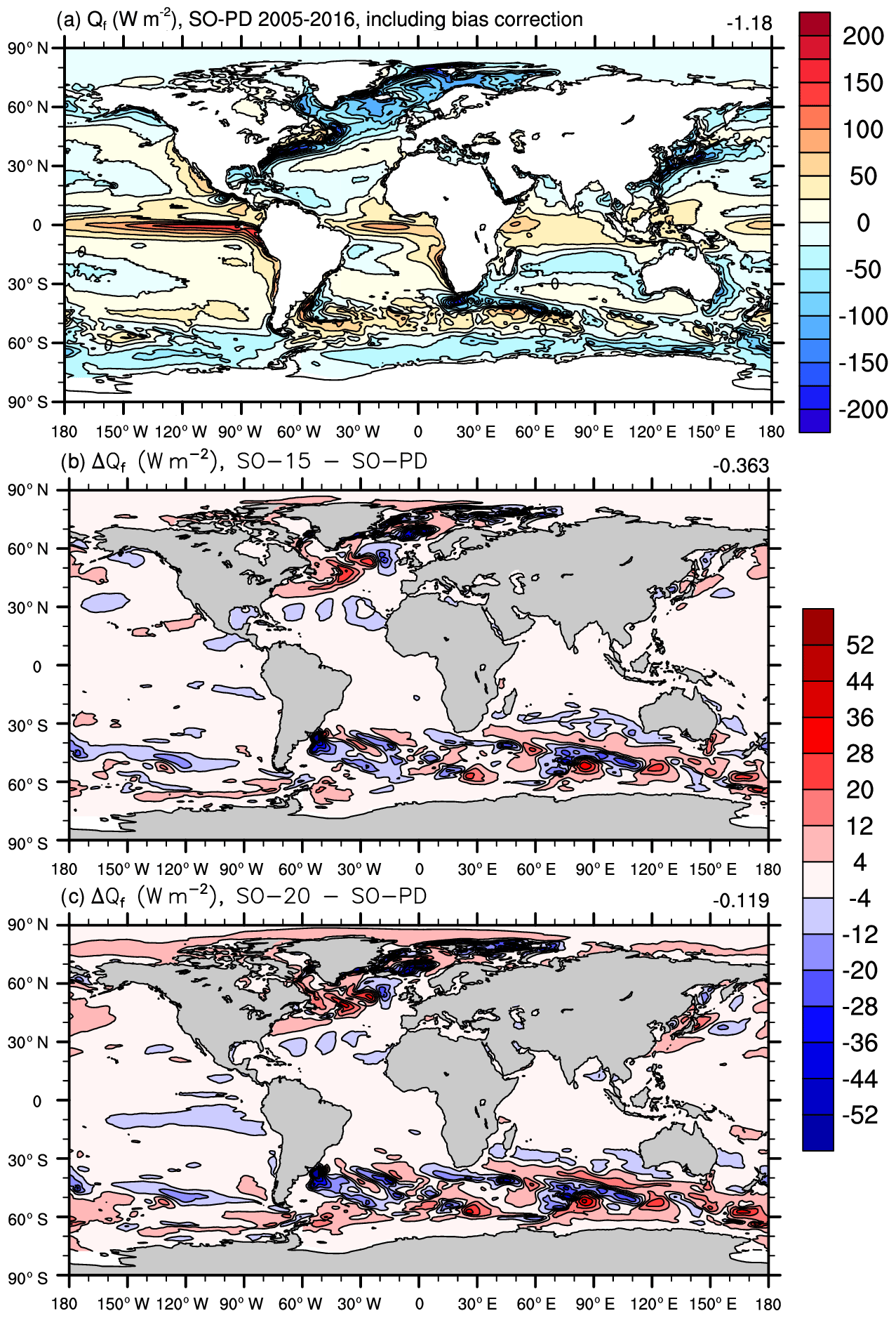
Figure 6 The annual-mean ocean heat flux (Q_f) needed in NorESM1-HappiSO to maintain a stable PD climate that is close to the observed SST used during calibration (a), and the change in Q_f for SO-15 (b) and SO-20 (c) compared to SO-PD. Negative values contribute to increasing SST (Eq. 1). Units are in W m⁻² (a–c).

Having determined the Q_f fields, we carried out 150-year simulations for SO-PD, SO-15, and SO-20. After a spin-up of 60 years, a new quasi-equilibrium is reached, giving three equilibrated periods of 90 years each (270 years in total).

The biases in the near-surface temperature for the PD climate are shown in Fig. 5b, e, h, and k (for the four seasons). While the biases are larger than those from AMIP-PD, they are still clearly reduced compared to CPL-PD. For instance, the global-mean bias in NH winter (December, January, and February; DJF) is reduced by 35 % in the SO and 64 % in AMIP model compared to the fully coupled model.

4 Temperature response

In what follows, we study the warming response in the 1.5 ^∘C experiment (with respect to PD) and the extra 0.5 ^∘C difference (between the 2.0 and 1.5 ^∘C experiments) from three versions of NorESM1-Happi: (1) NorESM1-HappiAMIP forced with prescribed SST and sea ice (Sect. 3.1); (2) NorESM-Happi, which is fully coupled (Sect. 3.2); (3) NorESM1-HappiSO, which has a SO model (Sects. 3.3 and 2.1). The disadvantage with the AMIP model is that it does not capture any ocean and sea-ice feedbacks. The coupled model on the other hand has larger biases, for instance, in near-surface temperatures (Fig. 5). The SO model offers an intermediate solution with smaller biases than the fully coupled model (Fig. 5), while still including feedbacks that are missing in the AMIP model setup. The AMIP experiments, however, comprise a much larger ensemble of experiments, which allows for establishing statistical significance of smaller trends (e.g. Li et al., 2018).

4.1 Temperature targets and the polar amplification factor

The changes in the global-mean near-surface temperature for the 1.5 and 2.0 ^∘C warmer worlds are given in Table 3. Note that these runs are designed to have temperature increases of 1.5 and 2.0 ^∘C relative to pre-industrial conditions, whereas we are comparing them to the PD climate, which is assumed to be 0.8 ^∘C warmer based on observations (Mitchell et al., 2017). Therefore, the target temperature increase between the PD experiments and the 1.5 and 2.0 ^∘C warming experiments is 0.7 and 1.2 ^∘C.

Table 3 The NH and SH polar amplification factor (NH-PAF and SH-PAF) and global-mean near-surface temperature (T_as) in the PD experiments and differences associated with 1.5 ^∘C warming, 2.0 ^∘C warming, and the 0.5 ^∘C difference for NorESM1-Happi, NorESM1-HappiSO, and NorESM1-HappiAMIP. PAF is defined as ΔT_Polar∕ΔT_Global, where T is the near-surface temperature, and the global and polar (poleward of 60^∘) subscripts indicate the averaging region.

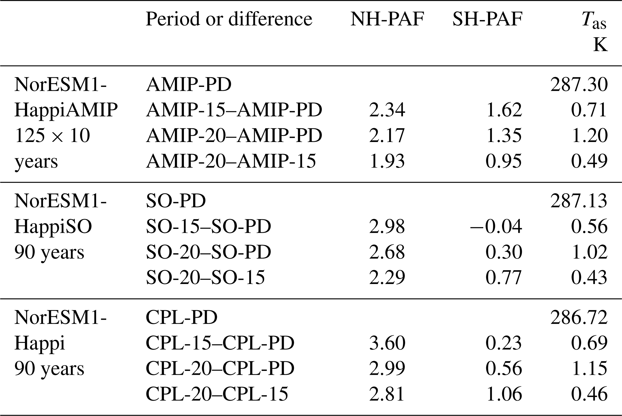
NorESM1-HappiAMIP hits the temperature targets of 0.7 and 1.2 ^∘C above PD temperatures quite accurately. The corresponding numbers are 0.56 and 1.02 ^∘C for NorESM1-HappiSO and 0.69 and 1.15 ^∘C for NorESM1-Happi. The warming compared to the PD climate is thus somewhat too low in the SO model, whereas it is closer to the targets in the fully coupled one. The difference between the 2.0 and 1.5 ^∘C warming experiments is quite similar across the models: 0.49 ^∘C for NorESM-HappiAMIP, 0.43 ^∘C for NorESM-HappiSO, and 0.46 ^∘C for NorESM1-Happi.

It is not entirely clear what is causing the smaller temperature response in the SO experiments, but we believe that it can mainly be attributed to the model's cold bias over the continents (Table 4; see discussion below) which is not adequately controlled by the adjusted ocean Q_f fluxes. As shown in the Supplement (Tables S3 and S4, as well as Figs. S5 and S7), the fully coupled model has a pronounced negative temperature bias which is stronger over continents than oceans. This can be related to generally underestimated cloudiness and to the strong meridional overturning circulation in the Atlantic Ocean (Figs. S14 and 4), which efficiently transfers heat into the deep ocean (Fig. 3) leaving less for surface heating. These properties are carried over to the SO model by the cloud properties of the atmospheric model and by the fluxes used to calibrate the future scenario states.

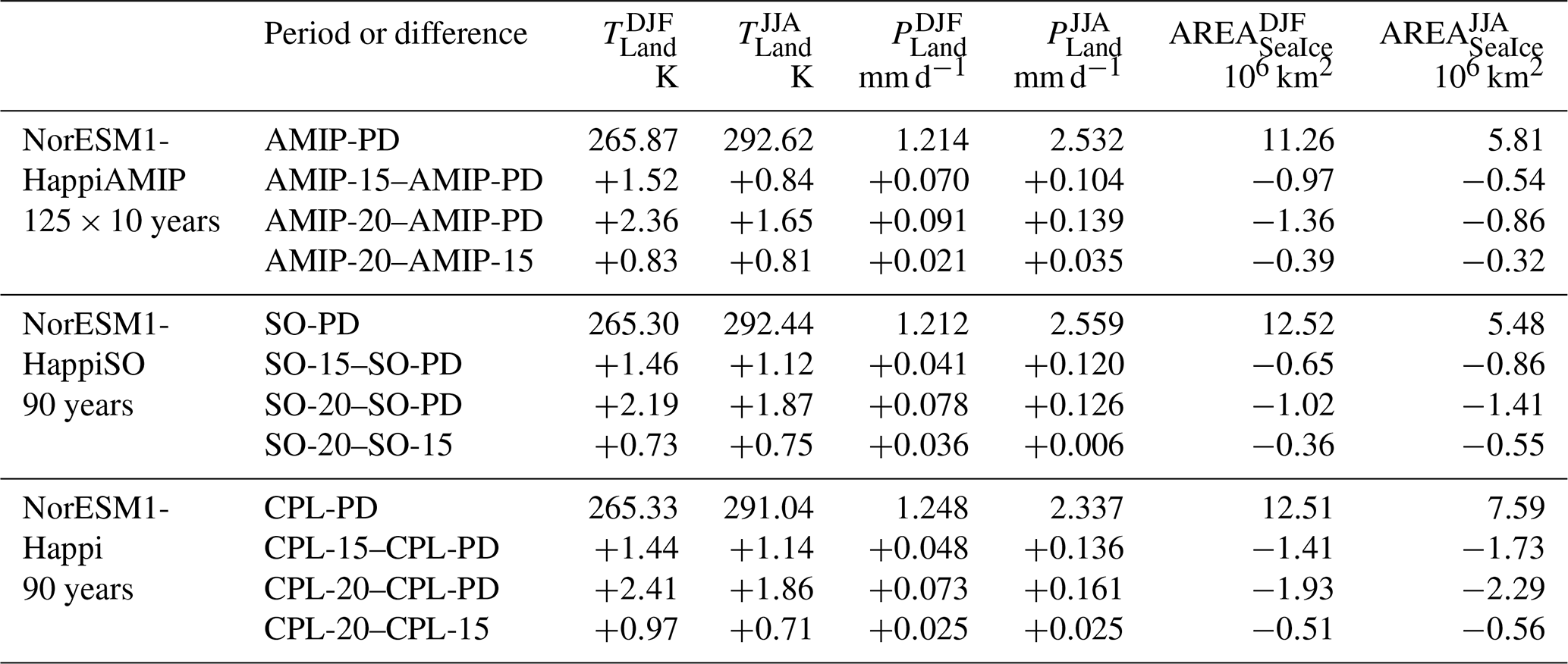
Table 4 Similar to Table 3 but for near-surface temperature over land, precipitation on land, and sea-ice area in the NH (20–90^∘ N) during winter (DJF) and summer (JJA).

The time evolution of the global-mean near-surface temperature response to 1.5 and 2.0 ^∘C warming in NorESM1-Happi is shown alongside the response for the Arctic region (area poleward of 65^∘ N) in Fig. 7. The temperature response is clearly amplified in the Arctic compared to the global mean. The ratio of the polar to the global near-surface temperature response defines the polar amplification factor (PAF; Table 3). The PAF is considerably larger in the Arctic than in the Antarctic, consistent with polar amplification being more pronounced in the NH. The Arctic amplification (NH-PAF) is, furthermore, stronger in the 1.5 ^∘C than in the 2.0 ^∘C warming scenarios.

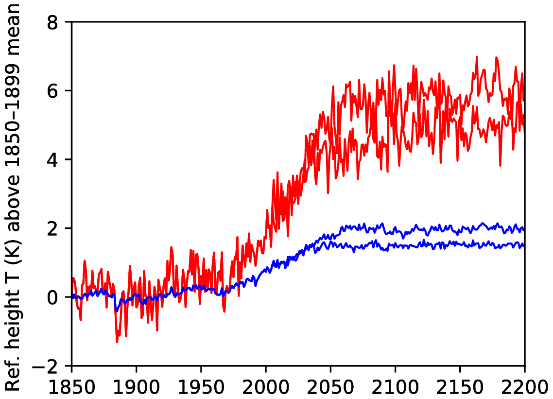
Figure 7 Time evolution of global-mean near-surface temperature for Hist1 (1850–2005) and CPL-15 and CPL-20 (2005–2200) from NorESM1-Happi relative to the 1850–1899 average. Fields are shown for the global average (blue) and for an average taken over the area north of 65^∘ N (red), i.e. approximately 4.7 % of the global area. Units are in Kelvin.

The Arctic amplification is enhanced in the experiments with an active ocean component. Compared to NorESM1-HappiAMIP, the Arctic amplification is 27 % stronger in the 1.5 ^∘C warmer world in NorESM1-HappiSO and 54 % stronger in NorESM1-Happi. With the additional 0.5 ^∘C warming, the Arctic amplification is 19 % and 46 % stronger in the SO and the fully coupled model than in the AMIP model.

To assess how the strength of the Arctic amplification in NorESM1-Happi compares to the CMIP5 models used for constructing the SST fields used in HAPPI (and thus in NorESM1-HappiAMIP), we have computed the PAF for RCP2.6 and RCP8.5 for each of the CMIP5 models. Results are shown in Fig. 8, along with the PAF for RCP2.6 and RCP4.5 for NorESM1-Happi, and for the different 1.5 and 2.0 ^∘C warming experiments. The figure shows that the PAF generally is larger in the NH than in the SH (consistent with Table 3), and that there is considerably more variability between the CMIP5 models when the forcing is weaker. Also, the CMIP5 multi-model median PAF is smaller for stronger forcing experiments (2.1 for RCP8.5 versus 2.4 for RCP2.6), in line with the results from the 1.5 and 2.0 ^∘C warming runs. The Arctic amplification in NorESM1-Happi is in the upper range of the CMIP5 models. For RCP2.6, the PAF for NorESM1-Happi is 3.4, which puts it above the median for the CMIP5 models (2.4) and somewhat below the 90th percentile (3.6).

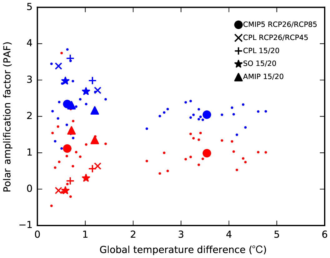
Figure 8 PAF versus the change in the global-mean near-surface temperature. Blue markers show values for NH and red markers for the SH. The small dots show the values for the CMIP5 models used in HAPPI, including NorESM1-M, for RCP2.6 (values with warming below 2 ^∘C) and RCP8.5 (values with warming above 2 ^∘C). The large dots show the CMIP5 multi-model means. Also shown are the values for NorESM1-Happi for RCP2.6 (left cross) and RCP4.5 (right cross), for CPL-15 (left plus sign) and CPL-20 (right plus sign), for SO-15 (left asterisk) and SO-20 (right asterisk), and for AMIP-15 (left triangle) and AMIP-20 (right triangle). For RCP2.6, RCP4.5, and RCP8.5, the PAF is computed by differencing the 10-year period (2091–2100) from the respective RCPs to 2006–2015 from RCP8.5 (as it is commonly used to extend the historical period beyond 2005). The values from the 1.5 and 2.0 ^∘C warming runs correspond to those in Table 3.

Table 4 shows similar statistics to Table 3 but for the NH extratropical (poleward of 20^∘ N) winter and summer land temperatures, land precipitation rates, and sea-ice area. The winter climate is colder over land in the fully coupled and SO models than in the AMIP model by −0.54 and −0.57 K, respectively. During summer, land temperatures are almost as high in the SO model as in the AMIP model, whereas the fully coupled model is 1.58 K colder. This is in line with the larger bias in the fully coupled model during this season (Fig. 5g–i).

The fully coupled model has the largest reduction in sea-ice area in the warmer climates during summer and winter. The SO model has larger changes than those prescribed in the AMIP model during summer and smaller changes during winter.

During summer, the SO model and the fully coupled model have the largest changes in land temperatures and precipitation in the 1.5 ^∘C warming experiment, whereas the AMIP model has the largest changes with the additional 0.5 ^∘C warming. During winter, the AMIP model has the largest changes in precipitation and temperature with the 1.5 ^∘C warming and the smallest changes in precipitation with the additional 0.5 ^∘C warming.

So far, we have considered changes in surface fields, but changes are also occurring aloft. Figure 9 shows the zonal-mean temperature response to the 1.5 ^∘C warming relative to the PD climate for NH winter (DJF) and NH summer (June, July, and August; JJA). There is upper-level warming in the tropics in all three models. The upper-level warming is somewhat more pronounced in the AMIP model and appears to be more consistent between the seasons than the Arctic amplification.

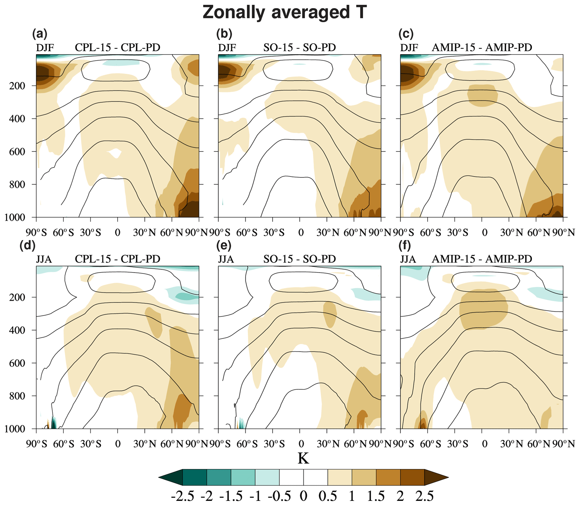
Figure 9 Zonal-mean temperature response relative to PD (colours) and climatology (solid black contours; 210 to 285 K in increments of 15 K) for the 1.5 ^∘C experiment from NorESM1-Happi (a, d), NorESM1-HappiSO (b, e), and NorESM1-HappiAMIP (c, f). Fields are shown for DJF (a–c) and JJA (d–f) for the default periods given in Sect. 3. Units are in Kelvin (a–f).

4.2 Equator-to-pole temperature gradients

The warming pattern in Fig. 9 is consistent with a sharpening of the upper-level Equator-to-pole temperature gradient and a weakening of the lower tropospheric gradient. Li et al. (2018) considered the multi-model mean changes in these gradients in five of the models contributing to the HAPPI project, including NorESM1-HappiAMIP. They found that the low-level gradient changes more with the initial 0.7 ^∘C warming (1.5 ^∘C – PD) than with the additional 0.5 ^∘C warming (2.0–1.5 ^∘C) in all the models. The upper-level gradient on the other hand strengthens more with the additional 0.5 ^∘C warming than with the initial 0.7 ^∘C, except in NorESM1-HappiAMIP where the changes are similar.

Figures 10 and 11 show the temperature gradients between the Equator and the North Pole at 200 and 850 hPa (e.g. Harvey et al., 2014) for the PD experiment and the 1.5 and 2.0 ^∘C warming experiments with NorESM1-Happi, NorESM1-HappiSO, and NorESM1-HappiAMIP, separated by season.

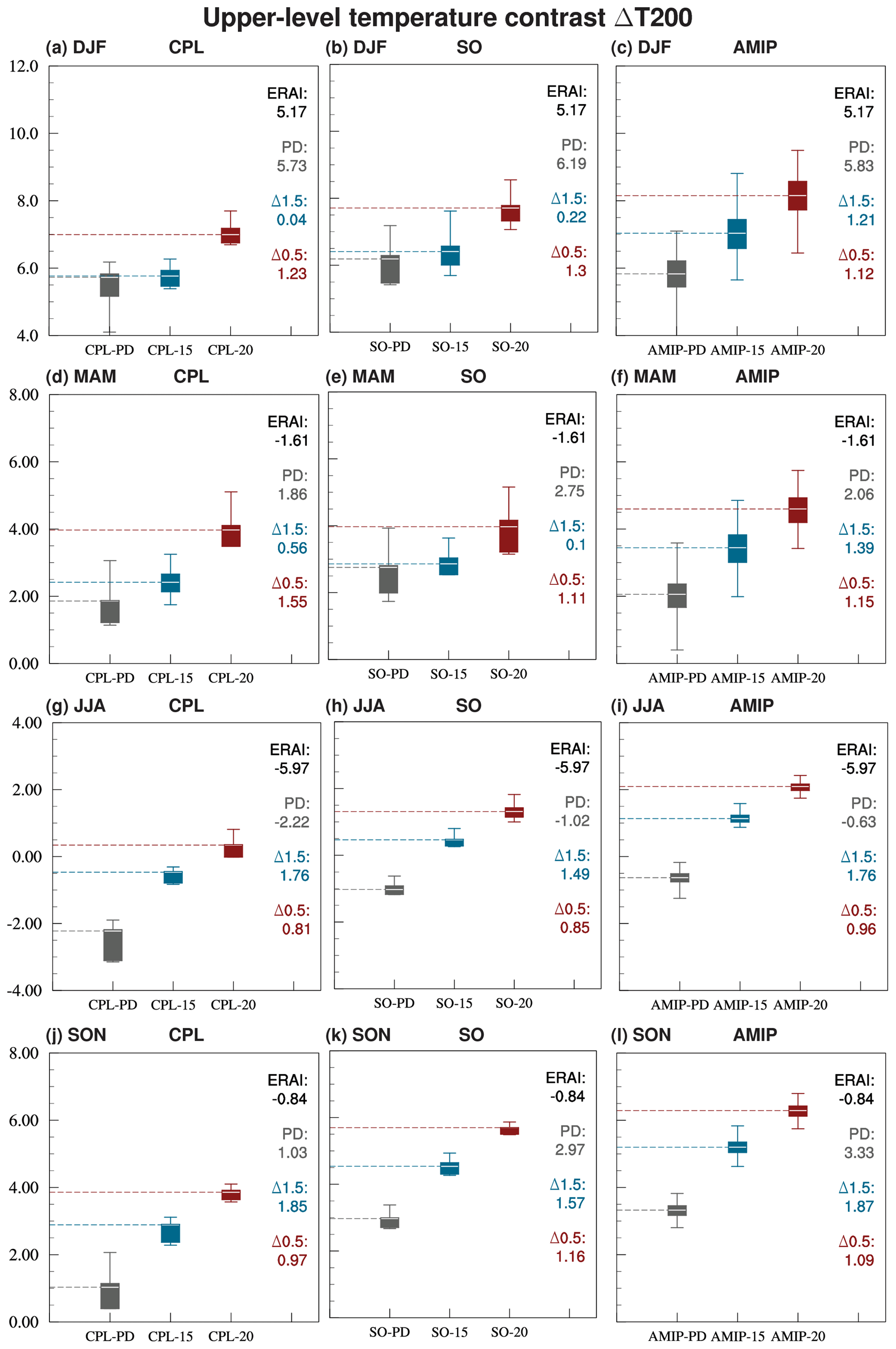
Figure 10 Upper tropospheric temperature contrast in the PD (grey), 1.5 ^∘C (blue), and 2.0 ^∘C (red) experiments from NorESM1-Happi (a, d, g, j), NorESM1-HappiSO (b, e, h, k), and NorESM1-HappiAMIP (e, f, i, l) for DJF (a–c), MAM (d–f), JJA (g–i), and SON (j–l). The upper-level temperature contrast (ΔT₂₀₀) is defined as the 200 hPa temperature difference between an area over the tropics (30^∘ S–30^∘ N) and an area over the Arctic (poleward of 60^∘ N). The white lines within the boxes indicate the median values, the boxes indicate the interquartile range, and the whiskers the full spread of the different decades in each experiment (nine in NorESM1-Happi, nine in NorESM1-HappiSO, and 125 in NorESM1-HappiAMIP). The dashed horizontal lines emphasize the median values; numbers are shown on the right side of each panel for ERA-Interim (top black), PD (second from top, grey), the change with 1.5 ^∘C warming relative to PD (third from top, blue), and the change with the additional 0.5 ^∘C warming (bottom, red). The ERA-Interim values are computed using the years 1986–2015. The NorESM data are for the default periods given in Sect. 3. Units are in degrees Celsius (a–l).

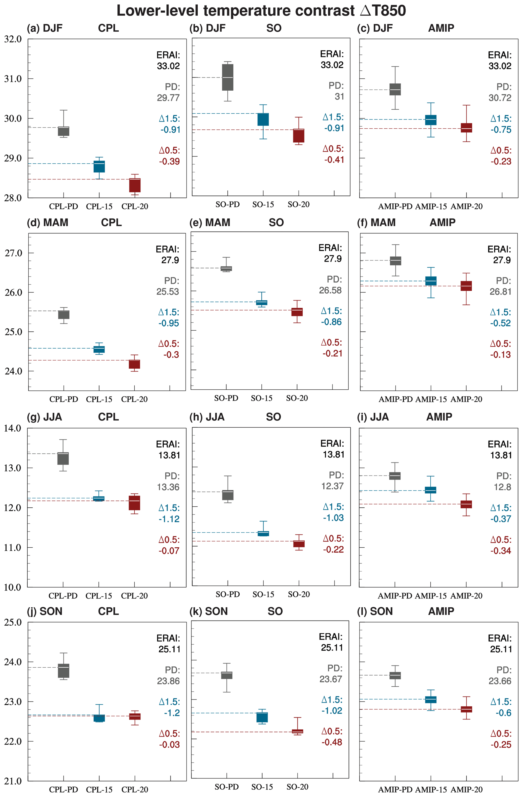
Figure 11 As in Fig. 10 but for the lower tropospheric temperature contrast at 850 hPa (ΔT₈₅₀).

The magnitude of the PD gradients is generally smaller in the fully coupled than in the SO and AMIP models, except during summer. While the fully coupled model might seem like an outlier, the upper-level gradient is actually closer to the one in ERA-Interim (Dee et al., 2011), indicating that the SO and AMIP models overestimate the upper-level pole-to-Equator temperature contrast (Fig. 10). At low levels, the fully coupled model underestimates the gradient during winter and spring (March, April, and May; MAM), while the gradients in the SO and AMIP models are stronger and closer to the reanalysis (Fig. 11). During summer (JJA) and fall (September, October, and November; SON), the fully coupled model has the smallest bias and the strongest contrasts at lower levels.

In line with the zonal-mean response in Fig. 9, the upper-level gradient generally increases with warming (Fig. 10), while the low-level gradient decreases (Fig. 11). The low-level gradient decreases more with the initial 0.7 ^∘C warming than with the additional 0.5 ^∘C, consistent with Li et al. (2018). Moreover, the decrease with the initial 0.7 ^∘C is larger in the fully coupled and SO models than in the AMIP model, consistent with the stronger Arctic amplification in these models (Table 3).

Changes in the upper-level gradient are less consistent across the experiments and seasons. There is little change with the initial 0.7 ^∘C warming in the fully coupled and SO models during winter and spring, while the gradient strengthens with the additional 0.5 ^∘C warming in all three models. During summer and fall, the upper-level gradient strengthens more with the initial 0.7 ^∘C warming than with the additional 0.5 ^∘C warming, like at low levels, only with no obvious differences between the model versions.

It is not clear why there is less warming aloft in the fully coupled model and SO model than in the AMIP model. It is possible that the cold biases in the tropics are contributing. As discussed above, both the fully coupled and the SO models are colder over land than the AMIP model during winter (Table 4), and the fully coupled model additionally has cold biases over the tropical oceans (Fig. 5).

5 Extratropical storm-track activity

Changes in the temperature gradients are known to be associated with changes in the extratropical storm tracks, with stronger gradients being associated with poleward shifts and weaker gradients with equatorward shifts (Brayshaw et al., 2008; Graff and LaCasce, 2012; Harvey et al., 2014; Shaw et al., 2016).

Extratropical storm tracks can be defined as regions of growing and decaying baroclinic waves embedded in the zones of pronounced meridional temperature gradient and mean westerly winds. Here, we represent the storm-track activity in terms of atmospheric fields, such as geopotential height, that have been bandpass filtered in time to isolate disturbances with timescales between 2.5 and 6 d (following Blackmon, 1976; Blackmon et al., 1977). The variability of the resulting fields is dominated by growing and decaying baroclinic waves, and the storm tracks are taken to be maxima in the bandpass-filtered variance fields (e.g. Blackmon et al., 1977; Chang et al., 2002, 2012).

Figure 12 shows the bias in the PD storm activity in terms of bandpass-filtered geopotential height at 500 hPa for NorESM1-Happi, NorESM1-HappiSO, and NorESM1-HappiAMIP. The fully coupled model underestimates the variability in all seasons. The bias is largest during winter over the North Atlantic on the equatorward side of the storm track and over the Nordic Seas, consistent with the North Atlantic storm track being overly zonal in NorESM (Iversen et al., 2013). The SO and AMIP models have both positive and negative biases over the storm-track regions and a North Atlantic storm track which extends too far downstream over central Europe.

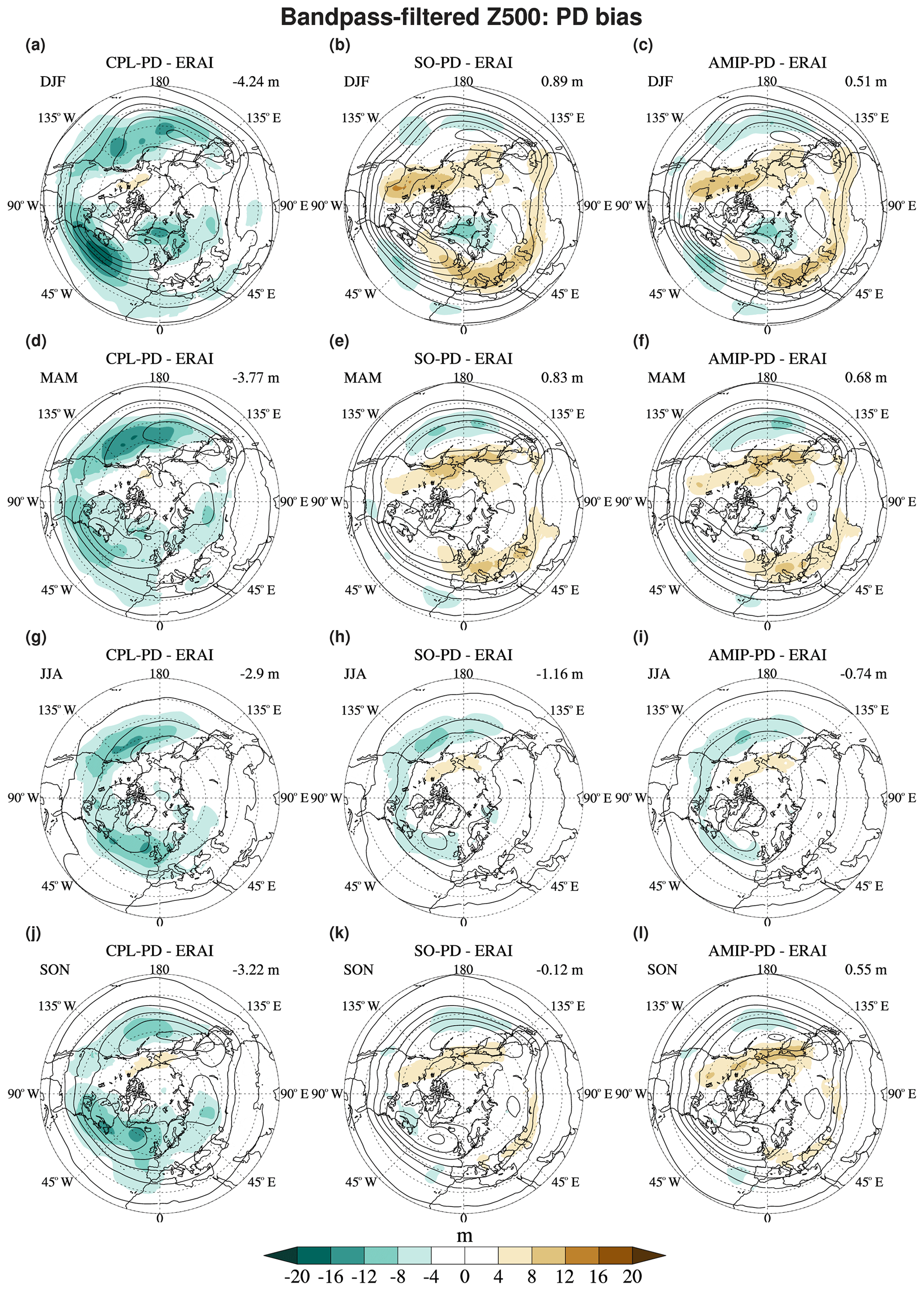
Figure 12 Upper-level storm-track bias relative to ERA-Interim (colours) and climatology (black contours; 8 to 70 m in increments of 8 m) for the PD experiment from NorESM1-Happi (a, d, g, j), NorESM1-HappiSO (b, e, g, k), and NorESM1-HappiAMIP (c, f, i, l) for DJF (a–c), MAM (d–f), JJA (g–i), and SON (j–l). The storm tracks are represented in terms of bandpass-filtered geopotential height at 500 hPa. The bias is computed relative to ERA-Interim for the years 1986–2015. The NorESM data are for the default periods given in Sect. 3. The numbers in the upper-right corners of each plot give the mean bias for the area shown on the plot (latitudes poleward of 20^∘ N). Units are in metres (a–l).

The storm-track biases are largest in the fully coupled model, whereas they are substantially smaller in the SO and AMIP models. The area-averaged winter bias for the region shown in Fig. 12 is, for instance, −4.24 m (13 % relative to ERA-Interim climatology) in the fully coupled model, 0.89 m (2.73 %) in the SO model, and 0.51 m (1.56 %) in the AMIP model.

Figures 13 and 14 show the changes in upper-level storm activity with the initial 0.7 ^∘C warming and with the additional 0.5 ^∘C warming for the three models and all four seasons. Li et al. (2018) found a poleward shift in upper-level storm activity with both the initial 0.7 ^∘C and the additional 0.5 ^∘C warming in the HAPPI multi-model ensemble. Here, the NorESM1-HappiAMIP model consistently displays more storm-track activity at high latitudes and less at lower latitudes with both warming scenarios, for all seasons. The exception is, as in Li et al. (2018), over the North Pacific, where there is an equatorward shift of during summer with the initial 0.7 ^∘C warming, and equatorward shift near the North American west coast region during winter with both the 0.7 ^∘C and the additional 0.5 ^∘C warming.

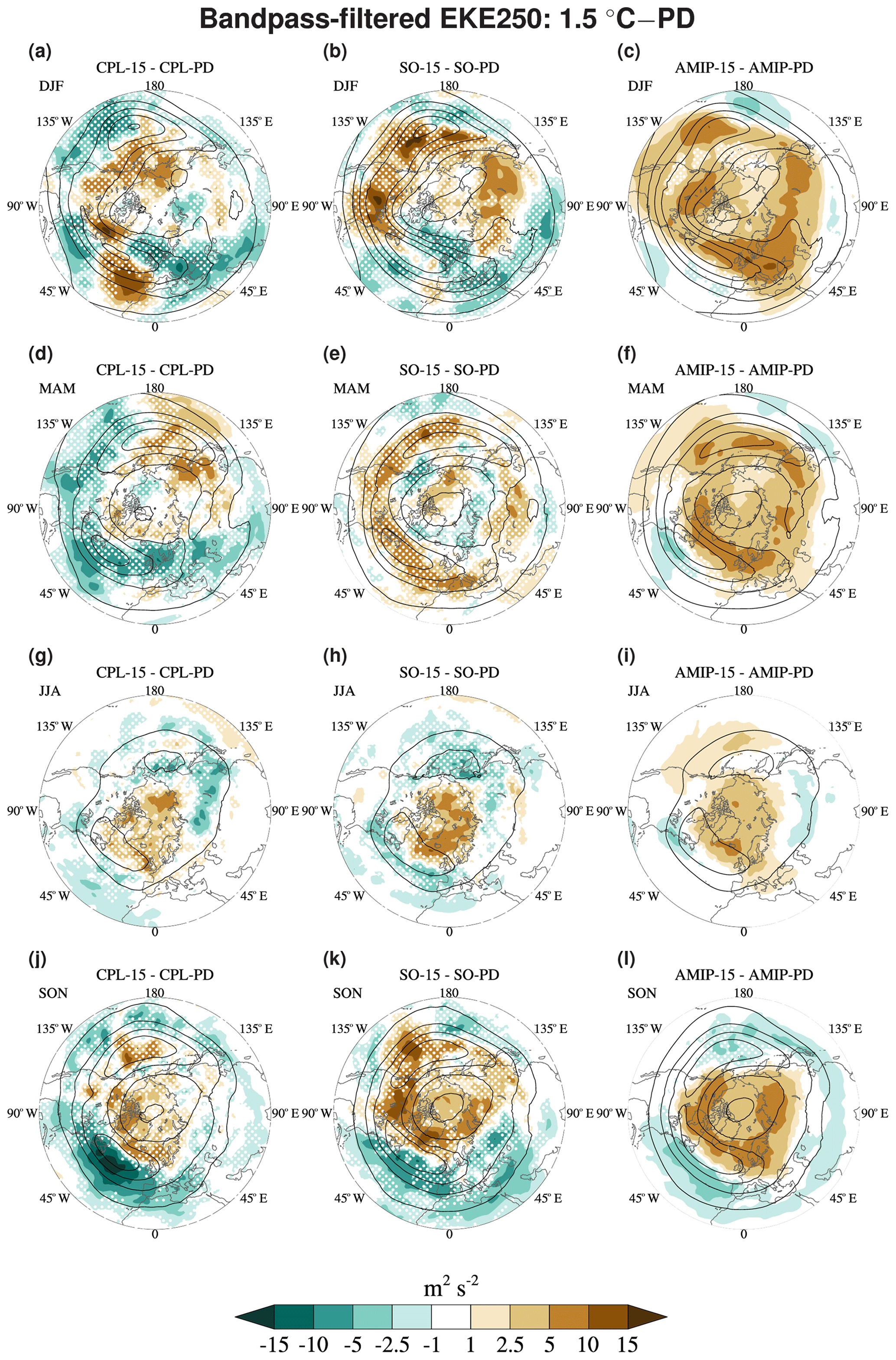
Figure 13 Changes in upper-level storm-track activity relative to PD (colours) and climatology (black contours; 40 to 240 m² s⁻² in increments of 40 m² s⁻²) for the 1.5 ^∘C experiment from NorESM1-Happi (a, d, g, j), NorESM1-HappiSO (b, e, h, k), and NorESM1-HappiAMIP (e, f, i, l) for DJF (a–c), MAM (d–f), JJA (g–i), and SON (j–l). The storm tracks are represented in terms of bandpass-filtered EKE (eddy kinetic energy) at 250 hPa. The white dots indicate that the differences are not significant at the 5 % level according to the Welch t test. The fields are shown for the default periods given in Sect. 3. Units are in m² s⁻² (a–l).

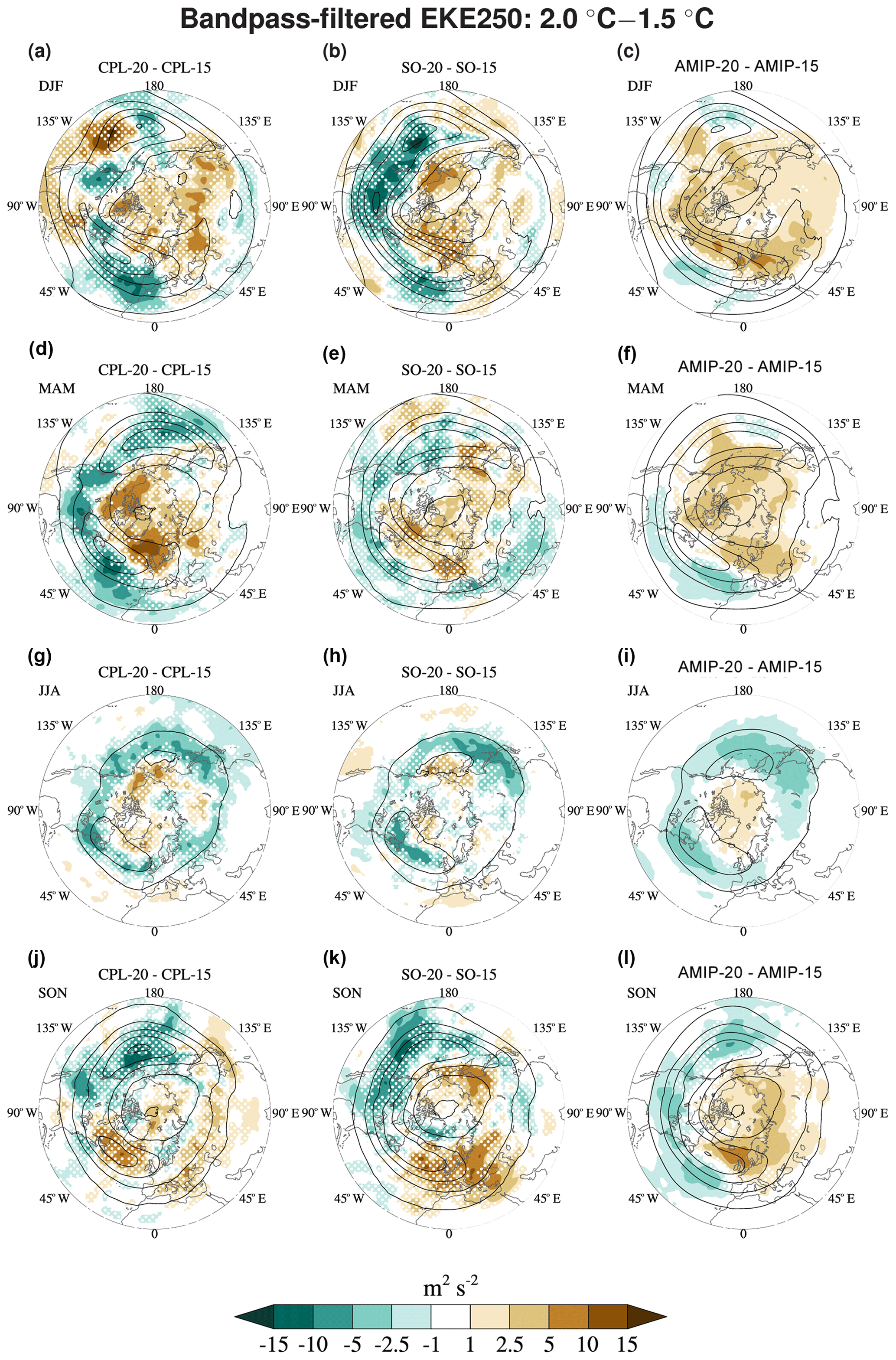
Figure 14 As in Fig. 13 but for the upper-level storm-track response to the additional 0.5 ^∘C warming (i.e. the difference between the respective 2.0 and 1.5 ^∘C experiments).

Changes in the fully coupled and the SO model are relatively consistent with those in the AMIP for the additional 0.5 ^∘C warming (Fig. 14). This is most clearly seen over the North Atlantic, where there tends to be more storm activity on the poleward side and less on the equatorward side. The poleward shift is in line with changes in the upper-level temperature gradient, which strengthens with the 0.5 ^∘C warming for all cases. Changes are, however, less consistent with the initial 0.7 ^∘C warming (Fig. 13). The response in the fully coupled and SO experiments resemble that in the AMIP experiments during summer and fall, with more activity at high latitudes and less at low latitudes. The reductions are, however, stronger for the fully coupled and the SO model. Changes during winter and spring are more complicated and do not particularly resemble those in the AMIP model.

Li et al. (2018) found the changes in the lower-level storm tracks to be less consistent and a similar conclusion can be drawn from the present results. We consider the low-level summer and winter storm tracks in terms of the meridional eddy heat flux. As in Li et al., the response to the initial 0.7 ^∘C warming (Fig. 15) is generally a reduction in storm-track activity, here indicating that the storm-track eddies are transporting less heat poleward. The decrease over the North Atlantic region is stronger in the fully coupled and the SO model than in the AMIP model. Changes during summer are weak. The response to the additional 0.5 ^∘C warming (Fig. 16) is also weak during summer. During winter, the AMIP and SO models have an increase southwest of the British Isles, but this is less pronounced (and not significant) in the fully coupled model. A similar increase is present in the multi-model mean in Li et al. (2018).

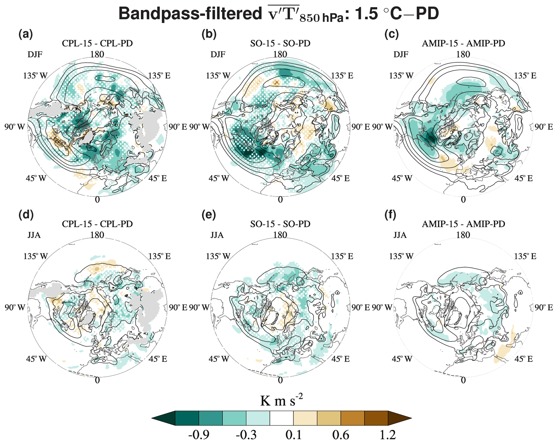
Figure 15 Changes in the low-level storm-track activity relative to PD (colours) and PD climatology (black contours; −12 to 12 K m s⁻² in increments of 4 K m s⁻²) for the 1.5 ^∘C experiment from NorESM1-Happi (a, d), NorESM1-HappiSO (b, e), and NorESM1-HappiAMIP (c, f) for DJF (a–c) and JJA (d–f). The storm tracks are represented in terms of the bandpass-filtered eddy heat flux $\stackrel{\mathrm{‾}}{v^{\prime }{T}^{\prime }}$ at 850 hPa. The white dots indicate that the differences are not significant at the 5 % level according to the Welch t test. The fields are shown for the default periods given in Sect. 3. Units are in K m s⁻² (a–f).

The white dots in Figs. 13–16 indicate that only the very strongest changes are significant in NorESM1-Happi and NorESM1-HappiSO, whereas the changes in NorESM1-HappiAMIP are more generally significant. This could be caused by the smaller number of model years available for the fully coupled and SO models, but it could also reflect a larger spread between the decades and members. While not all differences are significant, the similarity between certain aspects of the results from the AMIP experiments and the experiments with active ocean components does nonetheless increase our confidence in those aspects of the AMIP response.

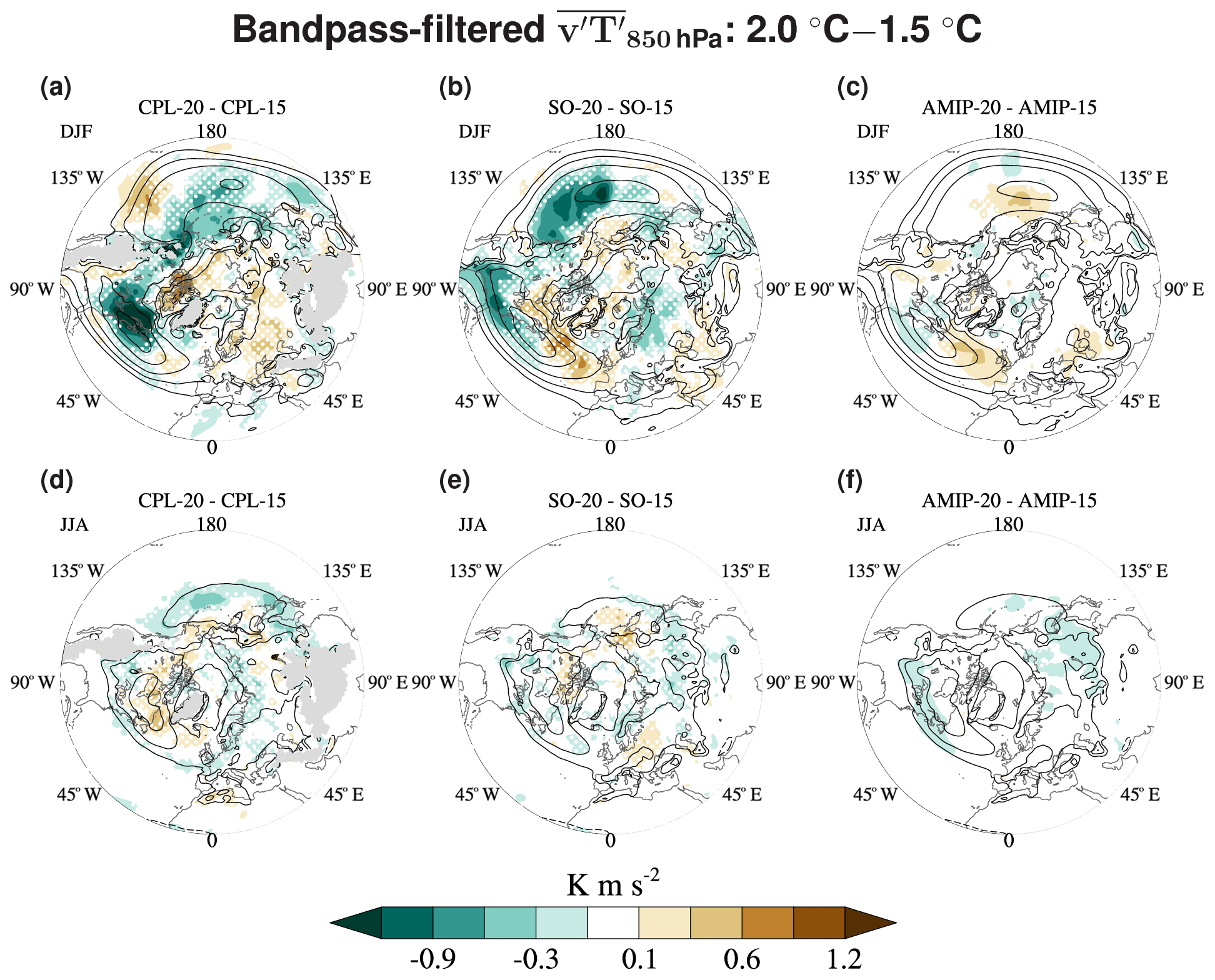
Figure 16 As in Fig. 15 but for the low-level storm-track response to the additional 0.5 ^∘C warming (i.e. the difference between the 2.0 and 1.5 ^∘C experiments).

6 Blocking frequency

Extratropical blocking is closely connected to persistent anticyclones, which can suppress precipitation at midlatitudes for periods of up to several weeks. The ability of climate models to simulate the occurrence of droughts at midlatitudes in the present and in future climates is conditioned by the models' ability to simulate blocking (e.g. Woollings et al., 2018).

Figure 17 shows the PD blocking frequency for NorESM1-Happi, NorESM1-HappiSO, and NorESM1-HappiAMIP for the winter and summer seasons. The blocking frequency is underestimated over the North Atlantic and western Europe during winter and over large parts of Eurasia during summer. The performance of the three models is generally similar, although some differences can be seen. The overestimation in NorESM1-Happi at 120^∘ W is, for instance, not as pronounced in the other two models. The SO and AMIP models perform slightly better over the Pacific, but the blocking occurrence is still underestimated in the Atlantic sector.

Figure 17 PD climatology of blocking frequency from NorESM1-Happi (a, b), NorESM1-HappiSO (c, d), and NorESM1-HappiAMIP (e, f) for DJF (a, c, e) and JJA (b, d, f). Shown are the mean (solid black line) and the spread (blue shading; ±1 SD) computed over the number of available decades (nine for NorESM1-Happi and NorESM1-HappiSO, and 125 for NorESM1-HappiAMIP) for the default time periods given in Sect. 3. Blocking frequency from ERA-Interim is shown for the period 1986–2015 (dotted black line). The blocking events are identified using the Tibaldi and Molteni (1990) blocking index with variable central latitude (vTM) (Tibaldi and Molteni, 1990; Pelly and Hoskins, 2003), as in Iversen et al. (2013). It is based on the TM index (Tibaldi and Molteni, 1990), which uses a persistent reversal of the meridional gradient of the 500 hPa geopotential height around the predefined central blocking latitude at 50^∘ N as an indicator for blocking. The reversal must be present at 7.5^∘ consecutive longitudes and persist for at least 5 d. In the vTM index, the requirement of a predefined central blocking latitude is relaxed in order to reduce spurious detection (Pelly and Hoskins, 2003). The central latitude is allowed to vary with longitude following the latitude of the maximum in the climatological storm track (using bandpass-filtered geopotential height at 500 hPa). To account for the seasonal cycle of the cyclone activity, the central latitude for a given month is calculated as the climatological 3-month moving average centred on that month. Units are percentages (a–f).

It is well established that many global climate models have problems simulating the occurrence and duration of blocking in the Euro-Atlantic sector and that the systematic errors are particularly large during NH winter. Several studies tie these problems to poor horizontal resolution, but there are likely other factors (Dawson et al., 2012; Davini and D'Andrea, 2016; Woollings et al., 2018).

The changes in the occurrence of winter and summer blocking in the 1.5 ^∘C warming experiment (relative to PD) and with the additional 0.5 ^∘C warming are shown in Fig. 18 for NorESM1-Happi, NorESM1-HappiSO, and NorESM1-HappiAMIP. The magnitude of the response varies dramatically between the models, and there is generally little consistency between the models regarding the sign and significance (indicated by the asterisk) of the response for the different longitudes. Although not shown, the same lack of consistency is also found for spring and fall.

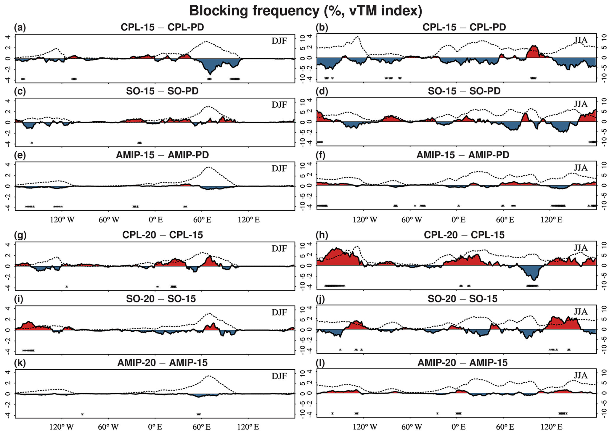
Figure 18 Change in blocking frequency (solid black line with red and blue shading) in the 1.5 ^∘C experiment relative to PD (a–f) and for the additional 0.5 ^∘C of warming (2.0–1.5 ^∘C; g–l), shown along with the blocking climatology for the PD experiment (dotted black line). The fields are shown for NorESM1-Happi (a, b, g, h), NorESM1-HappiSO (c, d, i, j), and NorESM1-HappiAMIP (e, f, k, l) during DJF (a, c, e, g, i, k) and JJA (b, d, f, h, j, l) for the default periods given in Sect. 3. The asterisks along the x axis indicate where the changes at that longitude are statistically significant at the 5 % level according to the Welch t test. Note that the left y axis is for the difference field and the right y axis is for the climatology. Units are percentages (a–l).

There are indications of more consistent changes between the model versions with the additional 0.5 ^∘C warming during NH summer, with increased blocking occurrence over parts of western Europe, the eastern Pacific, and the western Pacific. Changes are in these cases larger in the coupled models but most significant in the AMIP model. Note that the AMIP response can be statistically significant relative to the internal variability in the model, even though the amplitude of the response is small. Nevertheless, the results concerning NH blocking generally remain inconclusive.

7 Arctic sea-ice reduction

The extent, thickness, and concentration of sea ice are important properties of the climate system. Figure 19 shows the concentration of Arctic sea ice in March and September for NorESM1-Happi and NorESM1-HappiSO. For PD (Fig. 19a–d), the modelled concentrations are compared to remotely retrieved data from Ocean and Sea Ice Satellite Application Facility (OSI-SAF, 2017).

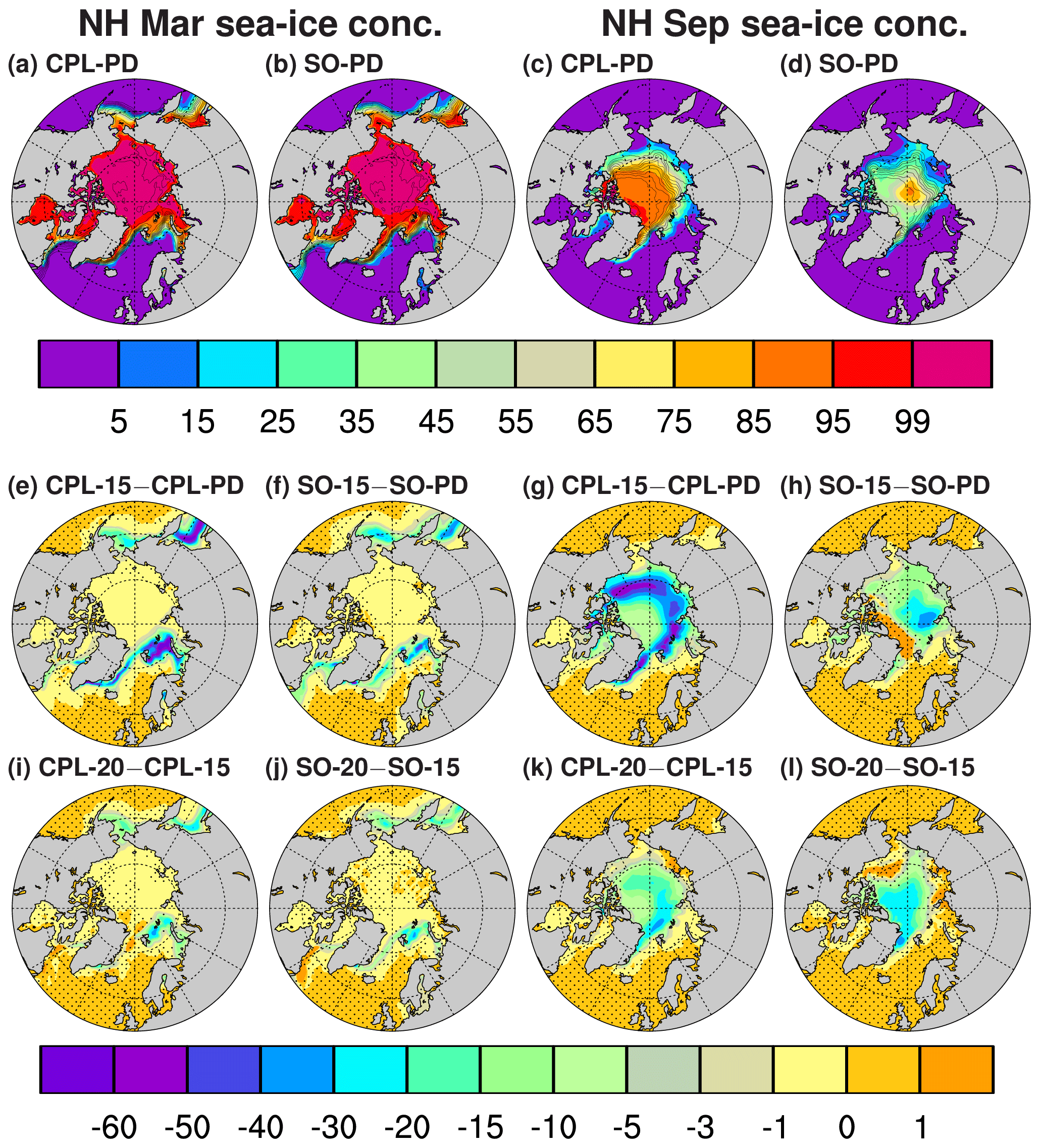
Figure 19 NH monthly-mean sea-ice concentrations for PD (a–d), the 1.5 ^∘C warming relative to PD (e–h), and the 0.5 ^∘C warming (i–l) from NorESM1-Happi (a, c, e, g, i, k) and NorESM1-HappiSO (b, d, f, h, j, l). Fields are shown for March (a, b, e, f, i, j) and September (c, d, g, h, k, l). The modelled concentrations are from the default 90-year periods (Sect. 3.2). The PD results (colours; top colour bar) are shown together with observational estimates (OSI-SAF, 2017; solid black contours) from 2006 to 2015. Differences that are not statistically significant at the 5 % level according to the Mann–Whitney U test are marked with black dots. Units are percentages of ocean surface area (a–l).

The quality of the model data is better in March than in September, when the SO model seems to underestimate the concentration, while the CPL-PD overestimates the ice cover. This is also seen when comparing the mean sea-ice extent to observations. For CPL-PD, the sea-ice extent in March/September (the numbers in parentheses are interannual standard deviations) is $\mathrm{14.26}\left(\mathrm{0.34}\right)/\mathrm{7.38}\left(\mathrm{0.62}\right)\times {\mathrm{10}}^{\mathrm{6}}$ km², while the observed for the relevant years (1996–2015) is $\mathrm{14.87}\left(\mathrm{0.36}\right)/\mathrm{5.71}\left(\mathrm{0.94}\right)\times {\mathrm{10}}^{\mathrm{6}}$ km². For the SO-PD, the March/September extent is $\mathrm{14.54}\left(\mathrm{0.36}\right)/\mathrm{4.22}\left(\mathrm{1.04}\right)\times {\mathrm{10}}^{\mathrm{6}}$ km² and the observed for the relevant time period (2005–2015) is $\mathrm{14.69}\left(\mathrm{0.33}\right)/\mathrm{5.04}\left(\mathrm{0.58}\right)\times {\mathrm{10}}^{\mathrm{6}}$ km². The March sea-ice cover seems to be rather well constrained by the gradients in SST, while summer extent is more influenced by local processes such as the albedo feedback associated with the contrasts between ice and open water.

From Table 4 (Sect. 4.1), we know that the NH winter sea-ice area is overestimated in CPL-PD and SO-PD compared with AMIP-PD which is based on observations. The reason for this is not fully understood. The PD climate in the fully coupled model is too cold with too-thick sea ice (not shown). This gives little summer melt and rather large sea-ice extent during early winter. For the SO-PD, the model is also cold during winter, but this can be related partly to the large ice cover. The use of annual-mean mixed layer depths in the SO model underestimates the mixed layer depth during autumn and winter. This might give too-low effective heat capacity in the ocean slab, which then causes too-rapid refreezing during autumn and early winter.

The sea-ice concentration is reduced in the warmer climates. In March, the largest changes occur along the edges of the ice (Fig. 19e–f and i–j). There is a larger reduction in the fully coupled than the SO model with the initial 0.7 ^∘C warming, whereas the changes are more similar with the additional 0.5 ^∘C. The changes occur over a larger fraction of the sea-ice-covered area in September (Fig. 19g–h and k–l) than in March. Changes are again larger with the 0.7 ^∘C than with the additional 0.5 ^∘C warming scenarios in the fully coupled model, whereas the sea-ice response to the 0.7 ^∘C and the 0.5 ^∘C warming scenarios is more similar in the SO model.

While the sea-ice concentration is reduced more with the warming in the fully coupled model, ice-free summers are more likely in the SO model. Figure 20 shows histograms of the relative occurrence of NH September sea-ice extent for NorESM1-Happi (Fig. 20a) and NorESM1-HappiSO (Fig. 20b). The sea-ice extent is shown for the observed and the modelled PD climate and the 1.5 and 2.0 ^∘C warming experiments. For PD climate, the SO model produces too few cases with the largest sea-ice extent, whereas the fully coupled model has too many. The overrepresentation in the latter case is likely caused by the cold bias in the model and the thick multi-year sea ice.

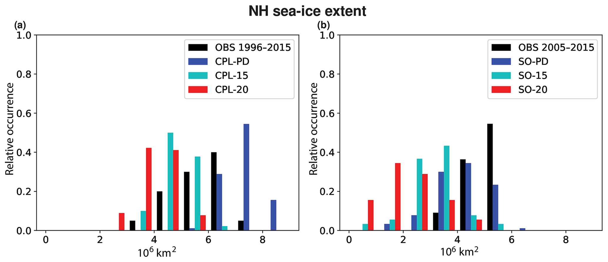
Figure 20 The relative occurrence of NH monthly-mean sea-ice extent in September for observations (black bars; OSI-SAF, 2017), the PD experiments (blue bars), and the 1.5 ^∘C (green bars) and 2.0 ^∘C warming experiments (red bars) from NorESM1-Happi (a) and NorESM1-HappiSO. The sea-ice extent is binned in 1.0×10⁶ km² increments. The observations are from 1996 to 2015 (20 values) in panel (a) and from 2005 to 2015 (11 values) in panel (b). The values from NorESM1-Happi and NorESM1-HappiSO are from the default 90-year periods (Sect. 3.2). Units are in 10⁶ km² (a, b).

The probability of having an ice-free Arctic in September, that is, a sea-ice extent between 0 and 1×10⁶ km², is practically zero for PD conditions in both models. The fully coupled model does not reach ice-free conditions with 1.5 ^∘C nor with 2.0 ^∘C warming (Fig. 20a). This is, perhaps, not surprising given that the model is too cold and has too much sea ice in the PD climate. So even though there are larger reductions in the sea-ice concentration in the fully coupled model, it does not produce an ice-free Arctic in September. Also, the interannual variability is smaller in the fully coupled model than in observations. We attribute this to the generally large sea-ice extent and thick multi-year ice. The model has a delayed Arctic sea-ice decline during the historical period compared with observations. The interannual variability in the model is comparable to that in observations in the period 1979–2004, before the recent rapid sea-ice decline.

Results are different for the SO model, which exhibits smaller biases in temperature and sea-ice extent. Ice-free September conditions are unlikely with 1.5 ^∘C warming, but the probability increases substantially to about 18 % with the additional 0.5 ^∘C warming (Fig. 20b). The difference between the two temperature targets is therefore potentially very large for the Arctic sea ice in summer and fall. The NorESM1-HappiSO tends to underestimate the relative occurrence of the highest sea-ice extent and overestimate the occurrence of the smaller extents in the PD climate (comparing the blue and black bars in Fig. 20a), which could indicate that there is an overestimation of ice-free conditions in the model. A substantial reduction in sea-ice extent between 1.5 and 2.0 ^∘C warming is, however, also seen in CESM1 (Sanderson et al., 2017; Jahn, 2018) and in CanESM2 (Sigmond et al., 2018).

8 Summary and discussion

In this paper, we focus on the response to global warming of 1.5 and 2.0 ^∘C relative to pre-industrial conditions in different versions of NorESM. We compare results from fully coupled and SO (slab-ocean) simulations to results from the AMIP-style simulations that were carried out for the multi-model HAPPI project (Mitchell et al., 2017; http://www.happimip.org/, last access: 14 September 2019). Because the AMIP runs are forced with prescribed SSTs and sea ice, they have small biases, but they also predefine important aspects of the Arctic amplification. The fully coupled and SO models allow for changes in SST and sea ice that can influence the surface albedo and atmospheric lapse rate, which are important elements in producing Arctic amplification (Pithan and Mauritsen, 2014). The motivation for using a SO model in addition to the fully coupled one is that the SO model has smaller biases, while still allowing the ocean and sea ice to respond to the forcing in the warming runs.

We consider the PD (present-day) climate, the response to the 0.7 ^∘C warming between the PD and the 1.5 ^∘C warming experiments (assuming 0.8 ^∘C warming between 1850 and PD), and the response to the additional 0.5 ^∘C warming between the 1.5 and 2.0 ^∘C experiments.

Results show that Arctic amplification, as measured by the PAF for the NH, is larger in the models with an active ocean component. In the fully coupled model, the PAF is 54 % stronger than in the AMIP model with the initial 0.7 ^∘C warming, and 46 % stronger with the additional 0.5 ^∘C warming. The difference is not as large for the SO model, which has 27 % and 19 % stronger PAF values for the same warming scenarios.

Arctic amplification weakens the lower tropospheric Equator-to-pole temperature gradient, and this decrease is larger with the initial 0.7 ^∘C warming than with the additional 0.5 ^∘C for all seasons. A similar result is also found in five HAPPI models (including NorESM1-HappiAMIP) studied by Li et al. (2018). The present study, however, shows that the changes with the initial 0.7 ^∘C warming are larger in the fully coupled and SO models than in the AMIP model, particularly during summer (JJA) and fall (SON).

The changes in the upper-level Equator-to-pole gradients are less consistent. The gradients generally increase with the warming because the tropics are warming aloft (e.g. Collins et al., 2013). During summer and fall, the upper-level gradient changes more with the initial 0.7 ^∘C warming, similar to the low-level gradient. The magnitude of the response is, however, not systematically larger in the experiments with an active ocean component. During winter and spring, the upper-level gradient changes very little with the initial 0.7 ^∘C warming in the coupled models and more with the additional 0.5 ^∘C, whereas the AMIP model has more similar changes with the 0.7 and 0.5 ^∘C warming. The changes in the upper-level gradient are also less consistent across the models than those in the low-level gradient in Li et al. (2018); while the upper-level gradient changes more with the additional 0.5 ^∘C in the multi-model mean, there is considerable spread among the models.

Changes in temperature gradients are known to be associated with changes in the storm tracks, with the tracks shifting poleward with stronger gradients and equatorward with weaker ones (Brayshaw et al., 2018; Graff and LaCasce, 2012; Harvey et al., 2014; Shaw et al., 2016). Li et al. (2018) identified poleward shifts in the multi-model mean upper-level storm tracks with the initial 0.7 ^∘C warming and with the additional 0.5 ^∘C warming. We find that while the AMIP model displays consistent poleward shifts in the upper-level storm activity with the initial 0.7 ^∘C warming for all seasons, the results from the coupled models are less consistent during winter and spring. The models agree more on the response to the additional 0.5 ^∘C. However, only the strongest changes in the fully coupled model and in the SO model are significant.

The low-level storm-track activity decreases with the initial 0.7 ^∘C warming. Changes with the additional 0.5 ^∘C warming are weak in the AMIP model, whereas the fully coupled and SO models have stronger reductions. All model versions have indications of more activity west of the British Isles, a response also seen in the multi-model mean in Li et al. (2018). These changes are, however, mostly not significant in the coupled models. To the extent that reduced low-level storm-track activity can be interpreted as slower propagation of cyclone waves in the westerlies, this can be associated with the reduced low-level temperature gradient associated with the high-latitude warming in the Arctic (e.g. Francis and Vavrus, 2012; Screen and Simmonds, 2013).

Our findings indicate that the storm-track response is not always very consistent between the model versions. There are, moreover, sizable biases in the storm tracks relative to reanalysis, especially in the fully coupled model. Barcikowska et al. (2018) provided a study of the Euro-Atlantic winter storminess which showed that modelling the regional atmospheric circulation, extreme precipitation, and winds with acceptable quality requires an atmospheric model with higher horizontal resolution (0.25^∘ in their study) than that used in the present study and in CMIP5 models.

The results for blocking activity remain for the most part inconclusive due to lack of consistency between the model versions and to the low statistical significance of the changes. Many aspects of blocking are also poorly simulated, likely because of the relatively coarse model resolution (Woollings et al., 2018).

The SO model simulates considerable differences in the reduction of sea ice in the Arctic between a 1.5 and 2.0 ^∘C warmer world. Ice-free summer conditions in the Arctic are estimated to be rare under 1.5 ^∘C warming, while occurring 18 % of the time under 2.0 ^∘C warming. This number may, however, be too high, as the SO model does tend to overestimate the relative occurrence of the smaller sea-ice extent and conversely underestimate the largest extent in the PD climate. A strong increase in the probability of having ice-free conditions when going from 1.5 to 2.0 ^∘C is nonetheless consistent with other studies (Jahn, 2018; Sigmond et al., 2018; Notz and Strove, 2018). The fully coupled model is too cold. It produces too much sea ice under PD conditions and is consequently not able to reach ice-free conditions in neither the 1.5 ^∘C nor the 2.0 ^∘C warming experiment, even though the changes from PD conditions are larger than for the SO model.

This paper does not discuss practical or scientific challenges that must be addressed in order to avoid exceeding certain temperature targets. Mathews et al. (2009) and Gillett et al. (2011) indicate that a constant equilibrium response in surface air temperature to anthropogenic CO₂ is determined by the accumulated carbon emissions. Hence, an ESM which calculates the atmospheric concentrations of CO₂ online from emissions should produce quite rapid stabilization of the global-mean surface temperature (e.g. Sigmond et al., 2018). This is possible if the ocean thermal inertia is balanced by decreasing atmospheric concentrations of CO₂ due to ocean uptake. NorESM1-Happi is not equipped with the possibility to run emission-driven GHG scenarios with online carbon cycling. Instead, the atmospheric concentrations of CO₂ are prescribed.

Results in this study show that there are important differences in the modelled response to 1.5 and 2.0 ^∘C warming in NorESM1-Happi depending on whether the model is run with prescribed SSTs and sea ice (AMIP), with the full ocean and sea-ice model, or with the sea-ice model coupled to a simplified ocean model. These differences could be due to the active sea-ice and ocean models allowing for feedbacks that are neglected in the AMIP runs, but they may also be affected by the experimental set up. Compared to the CMIP5 models, the Arctic amplification in NorESM1-Happi is in the high end of the range of responses. This indicates that the difference between the AMIP experiments and the ones with an active ocean model could have been smaller if the prescribed SSTs were based on results from NorESM1-Happi rather than those from the CMIP5 multi-model mean. More experiments are needed to understand this, such as those planned under PAMIP (Smith et al., 2019), to investigate the role of the background state.