the Creative Commons Attribution 4.0 License.
the Creative Commons Attribution 4.0 License.
 | 19 Mar 2019
Potential of global land water recycling to mitigate local temperature extremes
Mathias Hauser
Wim Thiery
Sonia Isabelle Seneviratne
Soil moisture is projected to decrease in many regions in the 21st century, exacerbating local temperature extremes. Here, we use sensitivity experiments to assess the potential of keeping soil moisture conditions at historical levels in the 21st century by “recycling” local water sources (runoff and a reservoir). To this end, we develop a “land water recycling” (LWR) scheme which applies locally available water to the soil if soil moisture drops below a predefined threshold (a historical climatology), and we assess its influence on the hydrology and extreme temperature indices. We run ensemble simulations with the Community Earth System Model for the 21st century and show that our LWR scheme is able to drastically reduce the land area with decreasing soil moisture. Precipitation responds to LWR with increases in mid-latitudes, but decreases in monsoon regions. While effects on global temperature are minimal, there are very substantial regional impacts on climate. Higher evapotranspiration and cloud cover in the simulations both contribute to a decrease in hot temperature extremes. These decreases reach up to about −1 ∘C regionally, and are of similar magnitude to the regional climate changes induced by a 0.5 ∘C difference in the global mean temperature, e.g. between 1.5 and 2 ∘C global warming.
- Article
(3822 KB) - Full-text XML
-
Supplement
(1714 KB) - BibTeX
- EndNote


Land water plays an important role in the development of temperature extremes and heatwaves. Changes in soil moisture (SM) can alter the amount of water that is available for evapotranspiration (ET), affecting local climate through its impact on the energy and water cycles (Seneviratne et al., 2010). The relationship between SM and temperature has been studied extensively in both observation-based (Hirschi et al., 2011; Whan et al., 2015) and model-based (Fischer et al., 2007; Lorenz et al., 2010; Hauser et al., 2016) studies.
Projections for the 21st century show decreasing SM in many mid-latitude regions (Orlowsky and Seneviratne, 2013; Berg et al., 2017), although the trends can differ substantially between models (Lorenz et al., 2016). The effect of future SM trends on temperature is typically assessed using idealized sensitivity experiments where SM is prescribed to predefined values, e.g. a climatology (Koster et al., 2004; Seneviratne et al., 2013; Hauser et al., 2017). In these climate model experiments, simulations with interactive SM are compared to simulations where SM is held at historical levels. A multi-model assessment found substantially reduced temperature extremes in projections with historical SM levels (Seneviratne et al., 2013; Lorenz et al., 2016; Vogel et al., 2017). A separate single-model experiment came to a similar conclusion, identifying that in regions which experience drying, the SM feedback is responsible for up to one-third of the projected increase in temperature extremes during the 21st century (Douville et al., 2016). However, these sensitivity experiments do not conserve water (Hauser et al., 2017), as moisture is artificially added or removed from the soil if it gets too dry or too wet.
More reality-based experiments on the potential effects of the land water cycle on climate can be obtained using simulations assessing the influence of irrigation. Irrigation is a land management practice that applies water to the soil, elevating SM levels. Therefore, irrigation does not only help sustain global food production, by providing agricultural crops the necessary water to grow, but it also influences local weather and climate. There are a number of studies investigating the impact of irrigation on climate utilizing global climate models (Sacks et al., 2009; Cook et al., 2011; Guimberteau et al., 2012; Krakauer et al., 2016; de Vrese et al., 2016; Hirsch et al., 2017; Thiery et al., 2017). For mean temperatures, most studies report a small cooling effect. However, temperatures often show an asymmetric response to irrigation. While local annual minimum temperatures (TNn) may slightly increase, the annual maximum (TXx) shows a much larger response than the mean. TXx was found to decrease by −0.78 ∘C averaged over all irrigated land area, whereas decreases of up to −2 ∘C were observed regionally (Hirsch et al., 2017; Thiery et al., 2017). The asymmetric effect of irrigation is because more water is applied during warm and dry periods, when the effect of SM on surface temperatures is especially pronounced (e.g. Schwingshackl et al., 2017). Therefore, irrigation has the potential to alleviate heatwaves, and it has been proposed that its potential effects on the local to regional scale should be better factored in within the context of mitigation and adaptation scenarios (Hirsch et al., 2017).
However, irrigation uses large quantities of water. The estimated global water consumption for irrigation has risen from approximately 600 km3 yr−1 in 1900 to more than 2000 km3 yr−1 in 2000 (Döll and Siebert, 2002; Wisser et al., 2010). Indeed, irrigation is responsible for 70 % of the global freshwater use by humans, and a large fraction of irrigation is realized using groundwater (Siebert et al., 2010; Döll et al., 2012). Overuse of this water resource can lead to groundwater depletion in intensely irrigated regions (Rodell et al., 2009, 2018; Famiglietti et al., 2011; Shamsudduha et al., 2012; Scanlon et al., 2012; Taylor et al., 2013). Given this unsustainable use of water, the question arises as to whether future generations will still be able to benefit from the climate impact of irrigation.
In this study we assess if it is possible to sustain historical SM levels in the 21st century without over-extracting local water resources. For this purpose, we develop a “land water recycling” (LWR) scheme that irrigates the soil if SM levels fall below late 20th-century conditions. The LWR scheme only uses local water sources; thus, water is only applied to the soil if it is available from runoff, and, potentially, a reservoir. We investigate if global-scale LWR is able to keep SM conditions at late 20th-century levels under future climate conditions and gauge its potential to mitigate local temperature extremes.
2.1 Model description
The Community Earth System Model (CESM, version 1.2, Hurrell et al., 2013) is a fully coupled Earth system model, developed at the National Center for Atmospheric Research (NCAR). This state-of-the-art model has been extensively evaluated (Hurrell et al., 2013; Meehl et al., 2013), and has been used to study irrigation (Sacks et al., 2009; Hirsch et al., 2017; Thiery et al., 2017) and SM–climate feedbacks using SM prescription (Koster et al., 2004; Seneviratne et al., 2013; Hauser et al., 2017). We employ the Community Atmosphere Model, version 5.3 (Neale et al., 2012), and the Community Land Model, version 4.0 (CLM4.0, Oleson et al., 2010; Lawrence et al., 2011), with a horizontal resolution of 1.9∘ × 2.5∘.
CLM4.0 is a third-generation land surface model (Sellers et al., 1997; Pitman, 2003), solving the energy and water balance of the land. The land surface is represented by five sub-grid land cover types (glacier, lake, wetland, urban, and vegetated), where the vegetation is represented by up to 16 plant functional types. The soil is represented by 15 layers with exponentially increasing depth. Of these 15 layers only the first 10 are hydrologically active, whereas the 5 deepest layers are only thermal slabs.
2.2 Land water recycling scheme
The aim of “land water recycling” (LWR) is to keep SM conditions above a certain threshold, but only if water from local sources is available. Therefore, we develop a LWR scheme by extending an existing SM prescription module (Hauser et al., 2017), as illustrated in Fig. 1. The LWR scheme adds water directly to each soil layer, analogously to drip-irrigation, using only water from runoff and, potentially, a reservoir. LWR is applied at every time step. First, the LWR scheme checks if SM is below the threshold. In this study, we use a historical SM climatology of the period from 1971 to 2000 as the threshold (Sect. 2.3). It is calculated as the median SM value at each grid cell, soil level, and day of the year. Next, the scheme checks if runoff is available and adds the required water to the soil, starting at the topmost layer. If the water demand can not be satisfied from runoff, the scheme then uses water from the reservoir, if available. In turn, runoff that is left after applying water to the soil is used to fill up the reservoir, if it is not yet full.
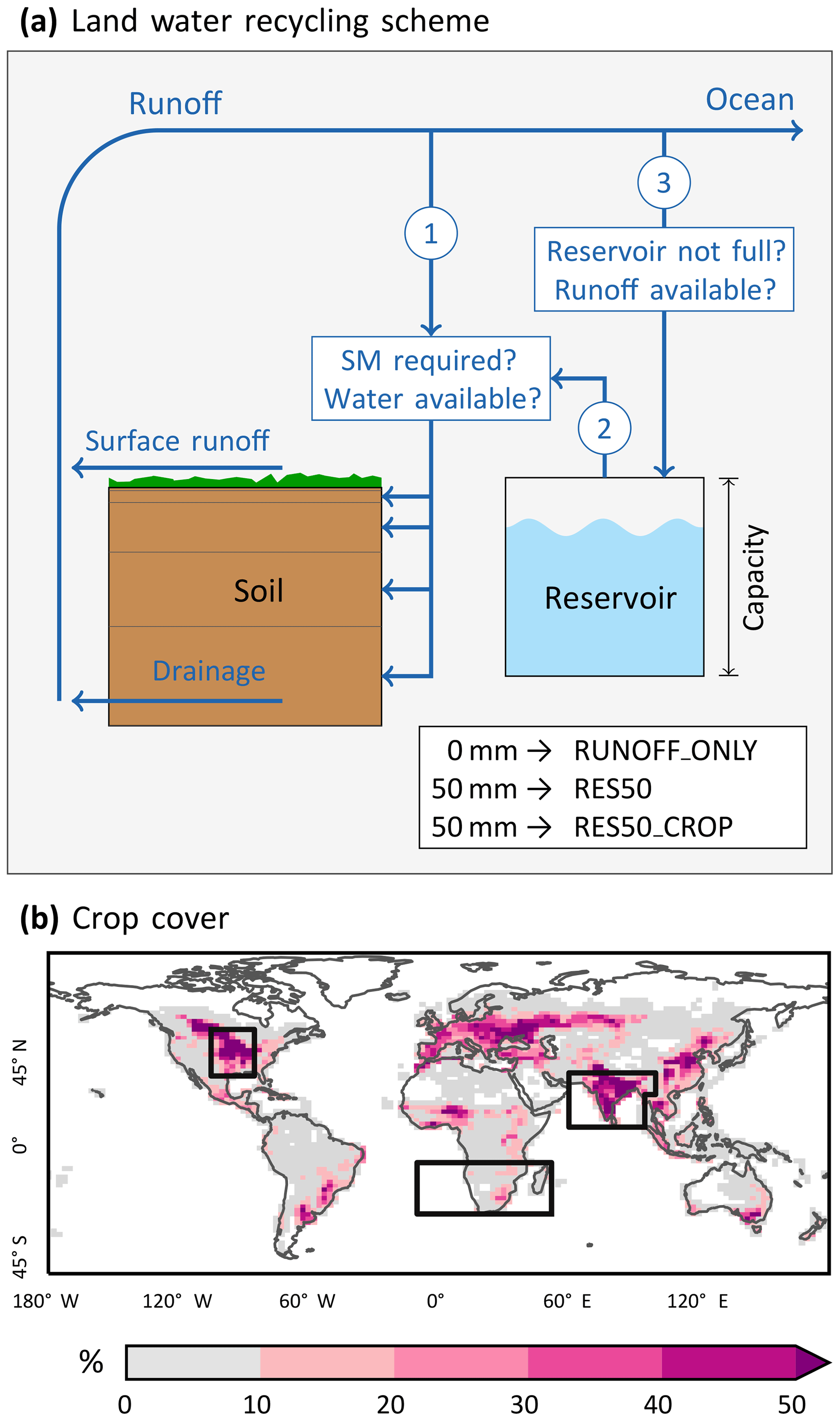
Figure 1Land water recycling (LWR) scheme, list of experiments, and area where LWR is applied in the RES50_CROP experiment (see Sect.2.3). (a) Illustration of the LWR scheme used in this study, and list of the reservoir capacity for each of the experiments. The blue lines indicate the “flow” of water in the algorithm: surface runoff is combined with sub-surface drainage resulting in total runoff. If SM is below the target threshold, this total runoff is used to water the soil (1). When not enough runoff is available, water is taken from the reservoir (2). Finally, any remaining runoff is then used to fill up the reservoir if necessary (3). Note that steps (2) and (3) are only carried out if the reservoir capacity is >0 mm. (b) Crop fraction in CLM in the year 2000. In RES50_CROP, LWR is applied in all grid cells with more than 10 % crop fraction. The black boxes in (b) show the three regions presented in Fig. 5: central North America (CNA), South Asia (SAS), and South Africa (SAF).
2.3 Experimental design
We use CESM to generate four climate ensembles that have three members each. The first ensemble is a reference simulation (REF), forced with historical “all forcing” conditions from 1850 to 2005, and prolonged until 2099 with the Representative Concentration Pathway 8.5 scenario (RCP8.5; Meinshausen et al., 2011). Each ensemble member is branched off a long pre-industrial control simulation at a different year. This equates to the standard CMIP5 set-up of CESM. The reference simulations use an interactive ocean model (the Parallel Ocean Program model, version 2) to simulate ocean dynamics.
We conduct three further ensembles, RUNOFF_ONLY, RES50, and RES50_CROP, which are also summarized using the term “experiments” (EXP). The experiments are branched off the reference simulations in 1950. In these simulations we apply the above-mentioned LWR scheme. The SM target (Sect. 2.2) is the climatology of the first ensemble member of REF.
In the first sensitivity experiment, RUNOFF_ONLY, water is only taken from the runoff in the same grid cell, i.e. the reservoir capacity is 0 mm (Fig. 1a). The second sensitivity experiment, RES50, includes a reservoir with a capacity of 50 mm at each grid cell. This allows for the transfer of a portion of the water in time (e.g. from a wet spring into a dry summer), and should therefore allow for a more reliable LWR. The size of the reservoir was chosen such that the resulting global reservoir capacity (6284 km3 yr−1) is close to the cumulative storage of human-made reservoirs as listed in the Global Reservoir and Dam (GRanD) database (6197 km3 yr−1) (Lehner et al., 2011). These first two sensitivity experiments are highly idealized in that they apply LWR globally to all vegetated and non-frozen land grid cells. Therefore, they gauge the potential of global-scale land water management. In a more realistic setting, the third sensitivity experiment, RES50_CROP10, is similar to RES50, but restricts LWR to all land areas with at least 10 % crop cover according to the vegetation map of CLM4.0 (Fig. 1b). Thus, in this experiment, LWR is mainly present in Europe, central North America, and India. All sensitivity experiments prescribe sea surface temperatures (SSTs) and sea ice from the respective REF ensemble member to suppress impacts from changes in SSTs in response to LWR.
2.4 Analysis
All analyses are carried out on the pooled ensemble members, either using annual values or the mean over the respective regions' warm season, defined here as the 3 warmest consecutive months. We determine the warm season in REF for a historical period (1971–2000). The warm season used generally corresponds to summer in mid- and high-latitude regions (Fig. S1 in the Supplement). However, other time frames are found in some other regions, e.g. in the tropics.
In our analysis we focus on the end of the 21st century and calculate 30-year climatologies for the period from 2070 to 2099. In light of the emerging literature on the effects of limiting global warming to 1.5 or 2.0 ∘C above pre-industrial levels we also analyse how our experiments fare compared to half a degree additional warming in the global mean temperature. To this end we assess how much of the additional local warming is compensated for by our sensitivity experiments. In particular, we calculate the relative cooling (or warming) of our experiments as follows:
where T* is a temperature index (see below), and 1.5 and 2.0 indicate the scenarios with 1.5 and 2.0 ∘C global warming, respectively. We do not have dedicated experiments to determine the response at 1.5 or 2.0 ∘C warming. Therefore, we select years where REF experienced a mean global warming of 1.5 ∘C ± 0.15 ∘C or 2.0 ∘C ± 0.15 ∘C (Fig. S2) with respect to 1861 to 1880. This selection criteria yields 19 years for the 1.5 ∘C scenario and 18 years for the 2.0 ∘C scenario.
To assess the influence of LWR on temperature extremes, we compute three indices from the daily model output. These indices are as follows: (i) the hottest daytime temperature of the year (TXx), measuring the intensity of heat extremes; (ii) the percentage of days that exceed the 90th temperature percentile (TX90p), i.e. the frequency of heatwaves; and (ii) the duration of the longest heatwave per year when the 3-day running mean exceeds the 90th temperature percentile (HWD), which is a measure of heatwave length. The 90th temperature percentile is calculated using the method from Zhang et al. (2005). We use a centred 15-day moving window for each calendar day of the year, pooling all three ensemble members. The 90th percentile is either calculated from the years 2070 to 2099, or 2023 to 2046 for the 1.5 ∘C versus 2.0 ∘C scenarios, such that the threshold and the exceedances are calculated for the same years.
Where appropriate, we test for significance with a Wilcoxon–Mann–Whitney U test (e.g. Wilks, 2011), as this test is suited for non-Gaussian data distributions (e.g. for TXx). We conduct a significance test at each grid cell, which leads to an increased probability of falsely rejecting the null hypothesis (e.g. Wilks, 2016). This problem is overcome by applying the correction described in Benjamini and Hochberg (1995), using a global p value of 5 %.
The influence of LWR on the surface temperature (TS) can be investigated with the help of the energy balance decomposition (Luyssaert et al., 2014; Akkermans et al., 2014; Thiery et al., 2015; Hirsch et al., 2017). Taking the derivative of the surface energy balance yields the contribution of each term to the LWR-induced change in TS:
where ϵ is the surface emissivity; σ is the Stefan–Boltzmann constant; SWnet is the net short-wave radiation; LWin is the incoming (downward) long-wave radiation; LH and SH are the latent and sensible head flux, respectively; and R is the residual term, which includes the ground heat flux. Δ stands for the difference between the experiments and the reference simulation (EXP–REF). We examine the energy balance for regions defined in the Special Report on Managing the Risks of Extreme Events (SREX) (Seneviratne et al., 2012). Thereby, we focus on the three following regions: central North America (CNA), South Asia (SAS), and South Africa (SAF), as shown in Fig. 1b.
3.1 Projected changes in soil moisture and hydrology
The LWR scheme only applies water to the soil if SM falls below the late 20th-century climatology. Therefore, it is of interest to assess the SM development in the 21st century. For the warm season, CESM projects a strong decrease in surface SM, especially in Europe, North America, South Africa, and north-eastern South America, whereas most other regions show a small to moderate increase (Fig. 2a). The response of CESM to climate change is consistent with the multi-model median projections from CMIP5 (Orlowsky and Seneviratne, 2013; Berg et al., 2017), with the exception of Australia; in Australia, the CMIP5 ensemble projects a SM decrease, whereas CESM shows a small increase. Nonetheless, CESM can be viewed as a representative member of the CMIP5 ensemble.
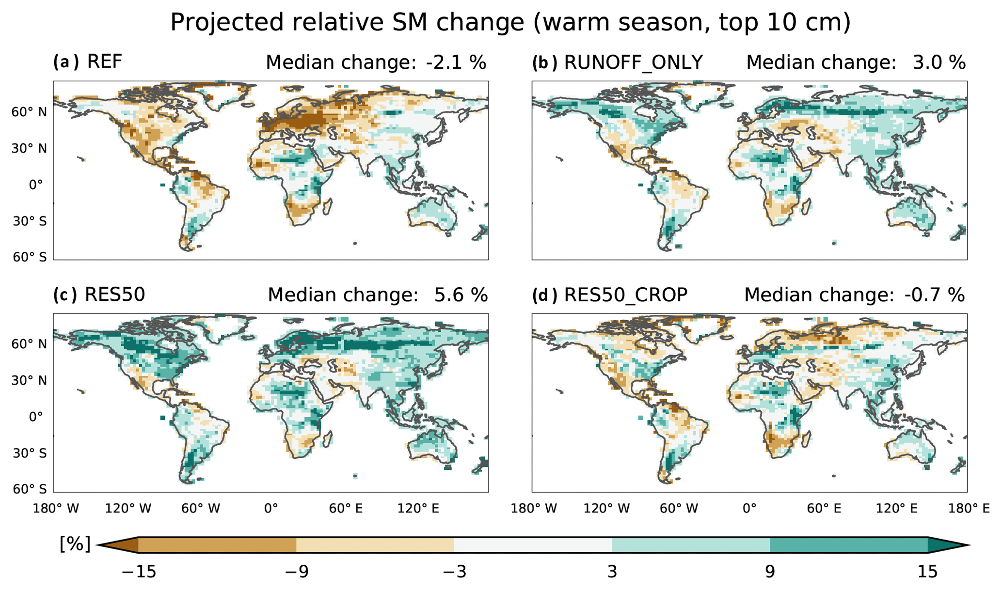
Figure 2Projected change of SM in the topmost 10 cm of the soil relative to the soil moisture climatology (1971 to 2000) in REF. Only the warm season (3 hottest consecutive months) is considered (Fig. S1).
LWR is able to substantially reduce the area with a negative SM trend (Fig. 2b–d). In RUNOFF_ONLY, SM increases by 3 % (spatial median), whereas in REF soils dried out overall (−2.1 %). It is mainly the increase of SM in Europe and North America which is responsible for this difference (Fig. 2b). Allowing for the storage of water for LWR further extends the area with a positive SM trend in the 21st century (Fig. 2c). Finally, in RES50_CROP SM is almost solely affected in areas where LWR is actually applied (not shown). This implies that there are no strong remote effects of LWR on SM. Overall, LWR is able to drastically reduce the fraction of days where the target SM conditions are not met (Fig. S3).
LWR is not only expected to influence SM, but also other components of the hydrological cycle. In our analysis we will concentrate on precipitation, ET, runoff, and the reservoir that is introduced. Comparing precipitation at the end of the 21st century between the experiments and REF reveals some distinct patterns (Fig. 3). Most areas in North America and Eurasia show a precipitation increase, whereas a large fraction of the tropics experiences a decrease. Partitioning this change into convective and large-scale precipitation shows that the former is responsible for the majority of the signal (Fig. S4). Averaged over all land areas, precipitation is lower due to LWR (Table 1). This is compensated for by increased precipitation over the oceans.
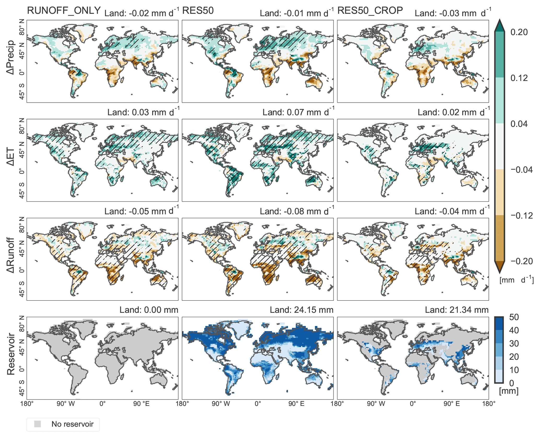
Figure 3Difference between EXP and REF for precipitation (Precip), evapotranspiration (ET), and runoff. The fourth row shows the mean reservoir state. Hatching in the first three rows indicates grid cells with significant changes (Wilcoxon–Mann–Whitney U test with a global p value of 5 %). Note that runoff values for the experiments can become zero, which leads to significant runoff changes in some regions with very small absolute changes.
The regions with decreasing precipitation coincide to a large degree with monsoon regions (as defined in Zhang and Wang, 2008). A decrease in precipitation in monsoon regions due to irrigation has been observed in earlier studies (Guimberteau et al., 2012; Puma and Cook, 2017; Thiery et al., 2017). It is consistent with a decrease in convective precipitation due to the cooling effect of water management (Sect. 3.2). The precipitation increase in the extratropics, in contrast, is likely due to the increased moisture input to the atmosphere, which can lead to an intensification of the local hydrological cycle. We have limited the analysis of extreme precipitation to annual maximum 1-day precipitation (Rx1day, Fig. S5). The changes detected in Rx1day between EXP and REF are generally smaller than 3 mm (15 %) and are nonsignificant. The spatial pattern closely follows the change of mean precipitation shown in Fig. 3.
Table 1Mean annual differences between EXP and REF for precipitation, ET, and runoff (in km3 yr−1).

An increase in ET is expected when adding water to the soil, which is confirmed in Fig. 3. This increase is present for almost all land areas, and ranges between 1000 and 4000 km3 yr−1, depending on the experiment (Table 1). This is clearly higher than estimates from irrigation studies for RUNOFF_ONLY and RES50 (e.g. 418 km3 yr−1 in Thiery et al., 2017; 1233 km3 yr−1 in Sacks et al., 2009). However, the LWR-induced ET surplus in RES50_CROP compares well with these previous model estimates.
Runoff is the only source of water for the LWR, for both direct water application and to fill the reservoir; thus, we generally expect a decrease. Indeed, global runoff decreases by approximately two-thirds of the annual discharge of the Amazon River (e.g. Gupta, 2008). However, there are some regions, mostly in the mid-latitudes, where the additional precipitation leads to a positive runoff signal (Fig. 3).
The long-term (2070 to 2099) average of the reservoir implies that the reservoir is either (almost) full or empty (Fig. 3). A spatial histogram also reveals a bimodal distribution with one peak below 1 mm and the other at 47 mm for RES50 and 39 mm for RES50_CROP (not shown). However, most grid cells have a seasonal cycle of more than 10 mm. Averaged over the whole SAS region, the reservoir contains 11 mm in the driest month, whereas there is twice as much water in the wettest month (23 mm). Similarly, the water in the reservoir fluctuates between 19 and 25 mm in CNA and between 7 and 20 mm in SAF. Thus, in many regions the reservoir is able to fulfil its function: providing water for LWR during the dry season.
3.2 Land water recycling effect on temperature
Next we turn our attention to the temperature effect of LWR. The global annual land temperature is reduced by −0.26, −0.42, and −0.23 ∘C for RUNOFF_ONLY, RES50, and RES50_CROP (for 2070 to 2099), respectively. This is more than a recent estimate (−0.05 ∘C) for realistic irrigation conditions (Thiery et al., 2017) during the period from 1981 to 2010, but similar to a comparable SM prescription scheme (−0.3 ∘C) (Hauser et al., 2017).
The effect of LWR on extreme temperature indices is shown in Fig. 4. The intensity, ΔTXx, is reduced by more than −0.46 ∘C over the global land area. Spatially, the reduction in TXx is more pronounced in the Northern Hemisphere than in the Southern Hemisphere, and Europe and central North America stand out as hotspots of LWR-induced cooling. This is in contrast to experiments with observed irrigation amounts, where India experiences a strong cooling (e.g. Thiery et al., 2017). This discrepancy can be explained by the soil moisture conditions in the historical period (1971 to 2000) and the projections (2070 to 2099). The soils in India are rather dry in the historical simulations and there is no strong drying in the projections (Figs. S6 and S9). Therefore, our simulations do not apply much water in this region, leading to a small effect on temperature. In contrast, the dry soils are the reason for the high irrigation rates in this region, which result in the very strong cooling, but come at the cost of strong groundwater depletion (Rodell et al., 2009).
For Europe and central North America, in comparison, REF indicates wet soils in the historical period and a strong drying in summer in the next century (Fig. S6). LWR is able to overcome this drying, especially when allowing for storage of water in a reservoir, causing the strong cooling in these regions. In historical irrigation simulations (as in Thiery et al., 2017) these regions do not receive as much water and therefore do not stand out as regions with a very strong cooling.
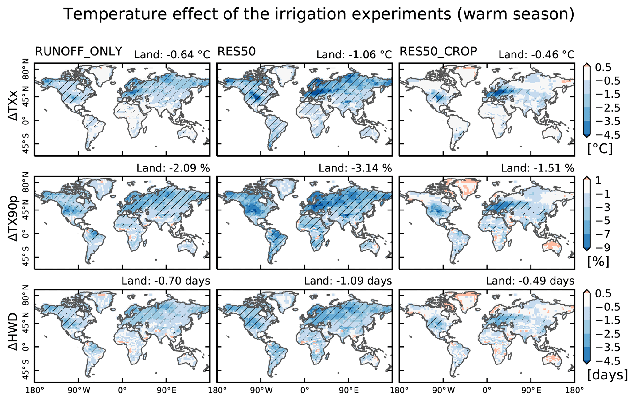
Figure 4Difference between REF and RUNOFF_ONLY (left column panels), RES50 (central column panels), and RES50_CROP (right column panels) for temperature indices. The top row represents TXx (intensity), the middle row represents TX90p (frequency), and the bottom row represents HWD (duration). Hatching indicates significant grid cells (Wilcoxon–Mann–Whitney U test with a global p value of 5 %).
For the next two indices (ΔTX90p and ΔHWD) we restrict the analysis to the warm season, as exceeding the 90th temperature threshold is not as relevant during the rest of the year. The change in the frequency of heatwaves (ΔTX90p) is between 1.51 % and 3.14 % when averaged over the whole land area (Fig. 4, middle row). Given that ΔTX90p is 10 % in REF (per definition), this is a substantial reduction. Indeed, in some regions the heatwave frequency is reduced to almost 0 % (not shown). Heatwaves do not only become less frequent, but they also become shorter. The average length of a heatwave (ΔHWD) is reduced by more than 0.5 days globally, and more than 3 days locally. For all three indices, it is evident that allowing for water storage leads to a stronger cooling: RES50 is colder than RUNOFF_ONLY for virtually all land areas.
To better understand the LWR-induced change in temperature, we make use of the energy balance decomposition (Eq. 2) introduced in Sect. 2.4. For CNA, there is a clear seasonal cycle in the surface temperature change (Fig. 5). The strongest cooling effect of LWR occurs during the warm season and shortly after. The energy balance decomposition reveals that changes in the radiative budget are mostly responsible for the decrease in temperature. The decrease in SWnet is caused by higher cloud cover (Fig. S7), which is in line with the observed increase in precipitation in this region (Fig. 3). The lower LWin, in comparison, is likely a response to the decreased boundary layer temperatures. Land–atmosphere feedbacks only really start to have an effect in July–September; that is, with a 1-month offset compared to the warm season (the 3 hottest months) considered . These are the months with the driest soil in this region (not shown) – only then are the higher SM levels able to increase the evaporative fraction and contribute to the cooling. Interestingly, the temperature response in RES50_CROP is smaller than in RES50, even though LWR is applied at almost all grid cells in RES50_CROP in this region (Fig. 1b). This may stem from a smaller cloud cover increase in RES50_CROP (Fig. S7), caused by the smaller water vapour input in other regions of the North American continent.
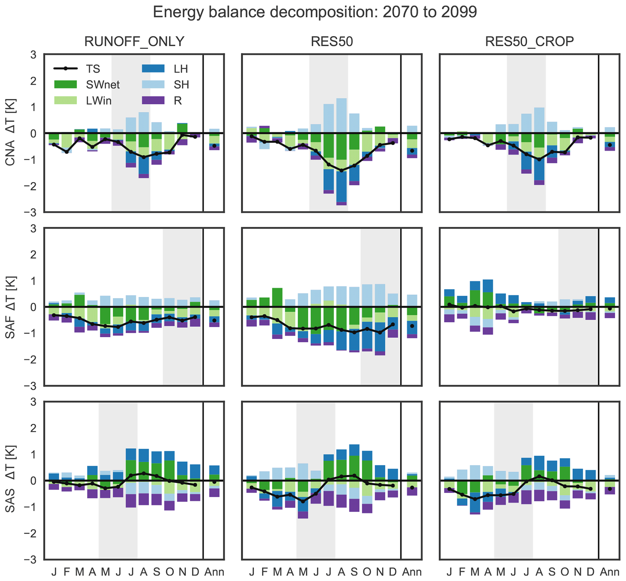
Figure 5The seasonal cycle and annual mean (Ann) of surface temperature anomalies and energy balance decomposition for central North America (CNA), South Asia (SAS), and South Africa (SAF). Grey shading indicates the warm season. TS stands for surface temperature, SWnet denotes net short-wave radiation; LWin denotes incoming (downward) long-wave radiation; LH and SH denote the latent and sensible head flux, respectively; and R is the residual term, which includes the ground heat flux.
SAF shows almost no seasonal cycle in TS and the contribution of the radiative- and land-terms of the energy balance seems to be more evenly distributed (Fig. 5). In RES50_CROP this region has almost no grid cells where LWR is applied (Fig. 1b); consequently, the temperature anomaly is small (−0.1 ∘C in the annual mean). Interestingly, the individual contributions are non-zero but compensate almost perfectly for one another. For the next region, SAS, the response in TS switches sign during the warm season. This change coincides with the SWnet reversing sign, which is consistent with the reduction of monsoon rainfall and the associated decrease in cloud cover.
We have shown that the LWR scheme developed in this study reduces extreme temperatures; however, this raises the question as to whether it was also able to offset half a degree increase in the global mean temperature. We answer this question in Fig. 6 with the help of Eq. (1): the blue denotes the percentage warming offset due to LWR, magenta indicates a warming in REF (), and light red shows where EXP is warmer than REF ().
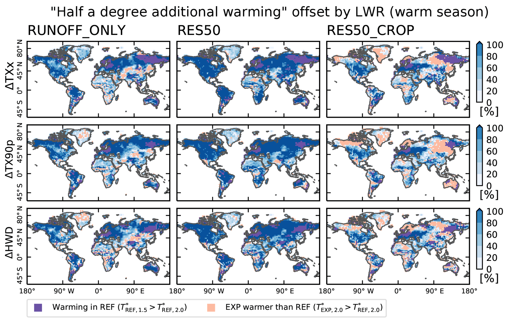
Figure 6Offset of half a degree additional global mean warming by the LWR experiments, see Eq. (1). Light red indicates regions where the LWR experiments are warmer than REF (for 2.0 ∘C global mean warming), magenta indicates regions where the 1.5 ∘C climate is warmer than the 2.0 ∘C climate in REF.
In RUNOFF_ONLY, LWR is able to offset the additional warming in parts of Eurasia, the Americas, and Australia, but not in Africa and South Asia. Allowing for water storage (RES50) leads to a larger area where the LWR-induced cooling dominates over global mean warming. However, temperatures in Africa and the southern parts of Asia still remain warmer. Finally, in RES50_CROP the cooling effect is mostly restricted to the LWR-areas in central North America and Europe.
Thus, our LWR scheme is able to locally offset the warming from half a degree additional warming. However, it does not change the general warming trend due to rising greenhouse gases, which are almost the same in the LWR experiments and REF (Fig. S8). This finding should be taken with caution, as we prescribe SSTs which will dictate the global mean warming. Nonetheless, they are in accordance with a similar study using an interactive ocean which also showed that the trend in regional temperatures is similar with and without irrigation throughout the 21st century (Hirsch et al., 2017).
In this study we used idealized climate model experiments to study the effect of sustainable global-scale land water management and its impact on temperature extremes. To this end, we developed a land water recycling (LWR) scheme that applies water to the soil if (i) it is drier than in the 1971 to 2000 median soil moisture climatology and if (ii) water is available from local sources.
We compute four sets of climate model experiments with the Community Earth System Model with three ensemble members in each. The four ensembles comprise a reference simulation and three sensitivity experiments including LWR. In the first sensitivity experiment, LWR only applies water to the soil if runoff from the same time step is available. In the second sensitivity experiment water is also taken from runoff, but a reservoir with a capacity of 50 mm is additionally available such that e.g. surplus water that accumulates during the wet season can be used for LWR in summer. Finally, the third sensitivity experiment also uses runoff and a reservoir as water sources, but only applies water in areas with a crop fraction of at least 10 %.
We have shown that LWR is able to maintain soil moisture conditions at late 20th-century levels for a large part of the global land area. However, LWR also has a marked impact on the hydrological cycle: it leads to an increase in precipitation in the mid- and high- latitudes, which is beneficial for areas where a precipitation decrease is projected for the next century. However, averaged over the global land area, this local increase is overcompensated for by a reduction in precipitation in monsoon regions. As expected, LWR leads to a large-scale increase in ET, due to higher soil moisture levels, and a decrease in runoff, as this is the only source of water applied. Further, the reservoir implemented is either “full” (>40 mm) or “empty” (<5 mm) in the long-term mean at most grid cells. Still, there is a strong seasonal cycle in the amount of water stored in the reservoir, indicating that it is able to provide water in the dry season.
LWR cools mean land air temperatures, but overall the effect is relatively small (−0.23 and −0.46 ∘C). For mid-latitude regions the cooling results from a combination of increased cloud cover and an increase of the evaporative fraction. In monsoon regions the decrease in precipitation is also associated with a decrease in cloud cover, which increases the amount of incoming solar radiation, offsetting part of the evaporative cooling. The impact of LWR on the upper end of the temperature distribution is larger. Annual maximum daytime temperatures, for example, decrease between −0.46 and −1.06 ∘C over all land areas, and the frequency and duration of heatwaves is strongly reduced. For many regions LWR leads to a stronger cooling than half a degree additional global mean warming.
Adding a reservoir generally leads to more LWR and thus strengthens the response of the climate. This is clearly visible in central and southern Europe, and central North America. Precipitation projections for the 21st century indicate a strong decrease in these regions during the warm season, but not for the whole year, which renders the reservoir especially effective. Restricting LWR to regions with at least 10 % crops, in comparison, mostly restricts the influence on these regions.
While applying a water management scheme that affects the whole land area is certainly unrealistic, these sensitivity experiments can place an upper limit on the potential of LWR to mitigate climate change. Certain irrigation modules impose no limit on the water available for irrigation (e.g. Oleson et al., 2013). Thus, a potential avenue for future development is to couple a more realistic irrigation scheme with the water resource limitations presented in this study. The third experiment, restricting LWR to crop areas, is a first step in this direction.
The LWR approach is sustainable in the sense that it does not use more water than locally available from runoff, and it does not lead to the depletion of groundwater reservoirs. However, our scheme imposes a large stress on runoff, leaving no residual flow in some regions. In practice this would have devastating ecological implications and would dramatically reduce river sediment transport (e.g. Chen et al., 2008). Additionally, some rivers are used for transport or to produce energy which would reduce the available water for LWR. Imposing a minimum flow condition is a potential important addition to the LWR scheme (Jaegermeyr et al., 2017), which is expected to decrease the response of the climate system. Further, a number of potential Earth system feedbacks arising from LWR are not considered in this study. For instance, LWR effects on hydrological processes, such as river temperature and salinity, water quality, sediment transport, groundwater extraction, and dam management, are not included in the current scheme; hence, they do not contribute to the overall climate feedbacks. In addition, we prescribe SSTs in our simulations, thereby disregarding potential feedbacks from the ocean. Performing simulations with an interactive ocean would, for instance, allow for the assessment of the influence of changes in salinity due to the LWR, and compare the effects of less river water inflow to the ocean, on the one hand, and enhanced precipitation and reduced evaporation over the ocean, on the other hand (Table 1). Finally, while the total reservoir capacity in our simulations compares well with observations, the spatial distribution of this reservoir capacity is highly irregular. Accounting for this heterogeneity would require the development of a dedicated map with a per-grid cell reservoir capacity. A more realistic representation of reservoirs could also be achieved by including evaporation from the reservoir (Lowe et al., 2009; Dingman, 2015) or by adding an explicit reservoir operation scheme (Hanasaki et al., 2006).
Overall, we were able to show that sustainable land water management is theoretically able to keep SM conditions at late 20th-century levels. Our study provides a new perspective on how land water can influence local and regional climate. While LWR only has a small influence on mean temperatures, it leads to a substantial decrease in extreme temperatures; thus, it can be seen as potential tool for local mitigation of climate change.
The code used is available at https://github.com/IACETH/prescribeSM_cesm_1.2.x (last access: 21 June 2018), where the documentation is also linked. The code is released under a MIT licence. Revision 67cf64 was used to conduct the simulations in this study with respect to land water recycling. Note that the model framework (and code) of CESM/CLM is necessary to compile and use the code available in the repository.
The supplement related to this article is available online at: https://doi.org/10.5194/esd-10-157-2019-supplement.
MH performed the majority of the analyses and wrote the paper with input from the co-authors. All authors participated in the design of the experiments and the discussion of the results.
The authors declare that they have no conflict of interest.
We thank Urs Beyerle for support with CESM. We acknowledge partial
support from the European Research Council (ERC) DROUGHT-HEAT project (contract 617518).
Edited by: Axel Kleidon
Reviewed by: two anonymous referees
Akkermans, T., Thiery, W., and Van Lipzig, N. P. M.: The Regional Climate Impact of a Realistic Future Deforestation Scenario in the Congo Basin, J. Climate, 27, 2714–2734, https://doi.org/10.1175/JCLI-D-13-00361.1, 2014. a
Benjamini, Y. and Hochberg, Y.: Controlling The False Discovery Rate – A Practical And Powerful Approach To Multiple Testing, J. Roy. Stat. Soc. Ser. B, 57, 289–300, 1995. a
Berg, A., Sheffield, J., and Milly, P. C. D.: Divergent surface and total soil moisture projections under global warming, Geophys. Res. Lett., 44, 236–244, https://doi.org/10.1002/2016gl071921, 2017. a, b
Chen, X., Yan, Y., Fu, R., Dou, X., and Zhang, E.: Sediment transport from the Yangtze River, China, into the sea over the Post-Three Gorge Dam Period: A discussion, Quatern. Int., 186, 55–64, https://doi.org/10.1016/j.quaint.2007.10.003, 2008. a
Cook, B. I., Puma, M. J., and Krakauer, N. Y.: Irrigation induced surface cooling in the context of modern and increased greenhouse gas forcing, Clim. Dynam., 37, 1587–1600, https://doi.org/10.1007/s00382-010-0932-x, 2011. a
de Vrese, P., Hagemann, S., and Claussen, M.: Asian irrigation, African rain: Remote impacts of irrigation, Geophys. Res. Lett., 43, 3737–3745, https://doi.org/10.1002/2016GL068146, 2016. a
Dingman, S. L.: Physical hydrology, Waveland Press, Long Grove, Illinois, 2015. a
Döll, P. and Siebert, S.: Global modeling of irrigation water requirements, Water Resour. Res., 38, 1037, https://doi.org/10.1029/2001WR000355, 2002. a
Döll, P., Hoffmann-Dobrev, H., Portmann, F. T., Siebert, S., Eicker, A., Rodell, M., Strassberg, G., and Scanlon, B. R.: Impact of water withdrawals from groundwater and surface water on continental water storage variations, J. Geodynam., 59–60, 143–156, https://doi.org/10.1016/j.jog.2011.05.001, 2012. a
Douville, H., Colin, J., Krug, E., Cattiaux, J., and Thao, S.: Midlatitude daily summer temperatures reshaped by soil moisture under climate change, Geophys. Res. Lett., 43, 812–818, https://doi.org/10.1002/2015GL066222, 2016. a
Famiglietti, J. S., Lo, M., Ho, S. L., Bethune, J., Anderson, K. J., Syed, T. H., Swenson, S. C., de Linage, C. R., and Rodell, M.: Satellites measure recent rates of groundwater depletion in California's Central Valley, Geophys. Res. Lett., 38, L03403, https://doi.org/10.1029/2010GL046442, 2011. a
Fischer, E. M., Seneviratne, S. ., Luethi, D., and Schaer, C.: Contribution of land–atmosphere coupling to recent European summer heat waves, Geophys. Res. Lett., 34, L06707, https://doi.org/10.1029/2006GL029068, 2007. a
Guimberteau, M., Laval, K., Perrier, A., and Polcher, J.: Global effect of irrigation and its impact on the onset of the Indian summer monsoon, Clim. Dynam., 39, 1329–1348, https://doi.org/10.1007/s00382-011-1252-5, 2012. a, b
Gupta, A.: Large rivers: geomorphology and management, John Wiley & Sons, Chichester, West Sussex, 2008. a
Hanasaki, N., Kanae, S., and Oki, T.: A reservoir operation scheme for global river routing models, J. Hydrol., 327, 22–41, https://doi.org/10.1016/j.jhydrol.2005.11.011, 2006. a
Hauser, M., Orth, R., and Seneviratne, S. I.: Role of soil moisture versus recent climate change for the 2010 heat wave in western Russia, Geophys. Res. Lett., 43, 2819–2826, https://doi.org/10.1002/2016GL068036, 2016. a
Hauser, M., Orth, R., and Seneviratne, S. I.: Investigating soil moisture–climate interactions with prescribed soil moisture experiments: an assessment with the Community Earth System Model (version 1.2), Geosci. Model Dev., 10, 1665–1677, https://doi.org/10.5194/gmd-10-1665-2017, 2017. a, b, c, d, e
Hirsch, A. L., Wilhelm, M., Davin, E. L., Thiery, W., and Seneviratne, S. I.: Can climate effective land management reduce regional warming?, J. Geophys. Res.-Atmos., 122, 2269–2288, https://doi.org/10.1002/2016JD026125, 2017. a, b, c, d, e, f
Hirschi, M., Seneviratne, S. I., Alexandrov, V., Boberg, F., Boroneant, C., Christensen, O. B., Formayer, H., Orlowsky, B., and Stepanek, P.: Observational evidence for soil-moisture impact on hot extremes in southeastern Europe, Nat. Geosci., 4, 17–21, https://doi.org/10.1038/NGEO1032, 2011. a
Hurrell, J. W., Holland, M. M., Gent, P. R., Ghan, S., Kay, J. E., Kushner, P. J., Lamarque, J. F., Large, W. G., Lawrence, D., Lindsay, K., Lipscomb, W. H., Long, M. C., Mahowald, N., Marsh, D. R., Neale, R. B., Rasch, P., Vavrus, S., Vertenstein, M., Bader, D., Collins, W. D., Hack, J. J., Kiehl, J., and Marshall, S.: The Community Earth System Model A Framework for Collaborative Research, B. Am. Meteorol. Soc., 94, 1339–1360, https://doi.org/10.1175/BAMS-D-12-00121.1, 2013. a, b
Jaegermeyr, J., Pastor, A., Biemans, H., and Gerten, D.: Reconciling irrigated food production with environmental flows for Sustainable Development Goals implementation, Nat. Commun., 8, 15900, https://doi.org/10.1038/ncomms15900, 2017. a
Koster, R., Dirmeyer, P., Guo, Z., Bonan, G., Chan, E., Cox, P., Gordon, C., Kanae, S., Kowalczyk, E., Lawrence, D., Liu, P., Lu, C., Malyshev, S., McAvaney, B., Mitchell, K., Mocko, D., Oki, T., Oleson, K., Pitman, A., Sud, Y., Taylor, C., Verseghy, D., Vasic, R., Xue, Y., Yamada, T., and Team, G.: Regions of strong coupling between soil moisture and precipitation, Science, 305, 1138–1140, https://doi.org/10.1126/science.1100217, 2004. a, b
Krakauer, N. Y., Puma, M. J., Cook, B. I., Gentine, P., and Nazarenko, L.: Ocean–atmosphere interactions modulate irrigation's climate impacts, Earth Syst. Dynam., 7, 863–876, https://doi.org/10.5194/esd-7-863-2016, 2016. a
Lawrence, D., Oleson, K., Flanner, M., Thorton, P., Swenson, S., Lawrence, P., Zeng, X., Yang, Z.-L., Levis, S., Skaguchi, K., Bonan, G., and Slater, A.: Parameterization Improvements and Functional and Structural Advances in Version 4 of the Community Land Model, J. Adv. Model. Earth Syst., 3, 1–27, https://doi.org/10.1029/2011MS000045, 2011. a
Lehner, B., Liermann, C. R., Revenga, C., Vörösmarty, C., Fekete, B., Crouzet, P., Döll, P., Endejan, M., Frenken, K., Magome, J., Nilsson, C., Robertson, J. C., Rödel, R., Sindorf, N., and Wisser, D.: Global reservoir and dam (grand) database, Tech. Doc. (ver. 1.1), NASA Socioeconomic Data and Applications Center, available at: http://sedac. ciesin. columbia. edu/data/collection/grand-v1 (last access: 21 June 2018), 2011. a
Lorenz, R., Jaeger, E. B., and Seneviratne, S. I.: Persistence of heat waves and its link to soil moisture memory, Geophys. Res. Lett., 37, L09703, https://doi.org/10.1029/2010GL042764, 2010. a
Lorenz, R., Argueeso, D., Donat, M. G., Pitman, A. J., van den Hurk, B., Berg, A., Lawrence, D. M., Cheruy, F., Ducharne, A., Hagemann, S., Meier, A., Milly, P. C. D., and Seneviratne, S. I.: Influence of land–atmosphere feedbacks on temperature and precipitation extremes in the GLACE-CMIP5 ensemble, J. Geopyhs. Res.-Atmos., 121, 607–623, https://doi.org/10.1002/2015JD024053, 2016. a, b
Lowe, L. D., Webb, J. A., Nathan, R. J., Etchells, T., and Malano, H. M.: Evaporation from water supply reservoirs: An assessment of uncertainty, J. Hydrol., 376, 261–274, https://doi.org/10.1016/j.jhydrol.2009.07.037, 2009. a
Luyssaert, S., Jammet, M., Stoy, P. C., Estel, S., Pongratz, J., Ceschia, E., Churkina, G., Don, A., Erb, K., Ferlicoq, M., Gielen, B., Grünwald, T., Houghton, R. A., Klumpp, K., Knohl, A., Kolb, T., Kuemmerle, T., Laurila, T., Lohila, A., Loustau, D., McGrath, M. J., Meyfroidt, P., Moors, E. J., Naudts, K., Novick, K., Otto, J., Pilegaard, K., Pio, C. A., Rambal, S., Rebmann, C., Ryder, J., Suyker, A. E., Varlagin, A., Wattenbach, M., and Dolman, A. J.: Land management and land-cover change have impacts of similar magnitude on surface temperature, Nat. Clim. Change, 4, 389–393, https://doi.org/10.1038/nclimate2196, 2014. a
Meehl, G. A., Washington, W. M., Arblaster, J. M., Hu, A., Teng, H., Kay, J. E., Gettelman, A., Lawrence, D. M., Sanderson, B. M., and Strand, W. G.: Climate Change Projections in CESM1(CAM5) Compared to CCSM4, J. Climate, 26, 6287–6308, https://doi.org/10.1175/JCLI-D-12-00572.1, 2013. a
Meinshausen, M., Smith, S. J., Calvin, K., Daniel, J. S., Kainuma, M. L. T., Lamarque, J.-F., Matsumoto, K., Montzka, S. A., Raper, S. C. B., Riahi, K., Thomson, A., Velders, G. J. M., and van Vuuren, D. P. P.: The RCP greenhouse gas concentrations and their extensions from 1765 to 2300, Climatic Change, 109, 213–241, https://doi.org/10.1007/s10584-011-0156-z, 2011. a
Neale, R. B., Chen, C.-C., Gettelman, A., Lauritzen, P. H., Park, S., Williamson, D. L., Conley, A. J., Garcia, R., Kinnison, D., Lamarque, J.-F., Marsh, D., Mills, M., Smith, A. K., Tilmes, S., Vitt, F., Morrison, H., Smith, P. C., Collins, W. D., Iacono, M. J., Easter, R. C., Ghan, S. J., Liu, X., Rasch, P. J., and Taylor, M. A.: Description of the NCAR Community Atmosphere Model (CAM 5.0), Tech. rep., National Center for Atmospheric Research, Boulder, Colorado, 2012. a
Oleson, K. W., Lawrence, D. M., Bonan, G. B., Flanner, M. G., Kluzek, E., Lawrence, P. J., Levis, S., Swenson, S. C., Thornton, P. E., Dai, A., Decker, M., Dickinson, R., Feddema, J., Heald, C. L., Hoffman, F., Lamarque, J.-F., Mahowald, N., Niu, G.-Y., Qian, T., Randerson, J., Running, S., Sakaguchi, K., Slater, A., Stöckli, R., Wang, A., Yang, Z.-L., Zeng, X., and Zeng, X.: Technical Description of version 4.0 of the Community Land Model (CLM), Tech. rep., National Center for Atmospheric Research, Boulder, Colorado, 2010. a
Oleson, K. W., Lawrence, D. M., Bonan, G. B., Drewniak, B., Huang, M., Koven, C. D., Levis, S., Li, F., Riley, W. J., Subin, Z. M., Swenson, S. C., Thornton, P. E., Bozbiyik, A., Fisher, R., Heald, C. L., Kluzek, E., Lamarque, J.-F., Lawrence, P. J., Leung, L. R., Lipscomb, W., Muszala, S., Ricciuto, D. M., Sacks, W., Sun, Y., Tang, J., and Yang, Z.-L.: Technical Description of version 4.5 of the Community Land Model (CLM), Tech. rep., National Center for Atmospheric Research, Boulder, Colorado, 2013. a
Orlowsky, B. and Seneviratne, S. I.: Elusive drought: uncertainty in observed trends and short- and long-term CMIP5 projections, Hydrol. Earth Syst. Sci., 17, 1765–1781, https://doi.org/10.5194/hess-17-1765-2013, 2013. a, b
Pitman, A.: The evolution of, and revolution in, land surface schemes designed for climate models, Int. J. Climatol., 23, 479–510, https://doi.org/10.1002/joc.893, 2003. a
Puma, M. J. and Cook, B. I.: Effects of irrigation on global climate during the 20th century, J. Geophys. Res.-Atmos., 115, D16120, https://doi.org/10.1029/2010JD014122, 2017. a
Rodell, M., Velicogna, I., and Famiglietti, J. S.: Satellite-based estimates of groundwater depletion in India, Nature, 460, 999–1002, https://doi.org/10.1038/nature08238, 2009. a, b
Rodell, M., Famiglietti, J. S., Wiese, D. N., Reager, J. T., Beaudoing, H. K., Landerer, F. W., and Lo, M.-H.: Emerging trends in global freshwater availability, Nature, 557, 651–659, https://doi.org/10.1038/s41586-018-0123-1, 2018. a
Sacks, W. J., Cook, B. I., Buenning, N., Levis, S., and Helkowski, J. H.: Effects of global irrigation on the near-surface climate, Clim. Dynam., 33, 159–175, https://doi.org/10.1007/s00382-008-0445-z, 2009. a, b, c
Scanlon, B. R., Faunt, C. C., Longuevergne, L., Reedy, R. C., Alley, W. M., McGuire, V. L., and McMahon, P. B.: Groundwater depletion and sustainability of irrigation in the US High Plains and Central Valley, P. Natl. Acad. Sci. USA, 109, 9320–9325, https://doi.org/10.1073/pnas.1200311109, 2012. a
Schwingshackl, C., Hirschi, M., and Seneviratne, S. I.: Quantifying Spatiotemporal Variations of Soil Moisture Control on Surface Energy Balance and Near-Surface Air Temperature, J. Climate, 30, 7105–7124, https://doi.org/10.1175/JCLI-D-16-0727.1, 2017. a
Sellers, P., Dickinson, R., Randall, D., Betts, A., Hall, F., Berry, J., Collatz, G., Denning, A., Mooney, H., Nobre, C., Sato, N., Field, C., and Henderson-Sellers, A.: Modeling the exchanges of energy, water, and carbon between continents and the atmosphere, Science, 275, 502–509, https://doi.org/10.1126/science.275.5299.502, 1997. a
Seneviratne, S. I., Corti, T., Davin, E. L., Hirschi, M., Jaeger, E. B., Lehner, I., Orlowsky, B., and Teuling, A. J.: Investigating soil moisture–climate interactions in a changing climate: A review, Earth-Sci. Rev., 99, 125–161, https://doi.org/10.1016/j.earscirev.2010.02.004, 2010. a
Seneviratne, S. I., Nicholls, N., Easterling, D., Goodess, C., Kanae, S., Kossin, J., Luo, Y., Marengo, J., McInnes, K., Rahimi, M., Reichstein, M., Sorteberg, A., Vera, C., and Zhang, X.: Changes in climate extremes and their impacts on the natural physical environment, in: book section 3, Cambridge University Press, Cambridge, UK and New York, NY, USA, 109–230, available at: http://www.ipcc.ch/report/srex/ (last access: 21 June 2018), 2012. a
Seneviratne, S. I., Wilhelm, M., Stanelle, T., van den Hurk, B., Hagemann, S., Berg, A., Cheruy, F., Higgins, M. E., Meier, A., Brovkin, V., Claussen, M., Ducharne, A., Dufresne, J.-L., Findell, K. L., Ghattas, J., Lawrence, D. M., Malyshev, S., Rummukainen, M., and Smith, B.: Impact of soil moisture-climate f eedbacks on CMIP5 projections: First results from the GLACE-CMIP5 experiment, Geophys. Res. Lett., 40, 5212–5217, https://doi.org/10.1002/grl.50956, 2013. a, b, c
Shamsudduha, M., Taylor, R. G., and Longuevergne, L.: Monitoring groundwater storage changes in the highly seasonal humid tropics: Validation of GRACE measurements in the Bengal Basin, Water Resour. Res., 48, W02508, https://doi.org/10.1029/2011WR010993, 2012. a
Siebert, S., Burke, J., Faures, J. M., Frenken, K., Hoogeveen, J., Doell, P., and Portmann, F. T.: Groundwater use for irrigation – a global inventory, Hydrol. Earth Syst. Sci., 14, 1863–1880, https://doi.org/10.5194/hess-14-1863-2010, 2010. a
Taylor, R. G., Scanlon, B., Döll, P., Rodell, M., van Beek, R., Wada, Y., Longuevergne, L., Leblanc, M., Famiglietti, J. S., Edmunds, M., Konikow, L., Green, T. R., Chen, J., Taniguchi, M., Bierkens, M. F. P., MacDonald, A., Fan, Y., Maxwell, R. M., Yechieli, Y., Gurdak, J. J., Allen, D. M., Shamsudduha, M., Hiscock, K., Yeh, P. J. F., Holman, I., and Treidel, H.: Ground water and climate change, Nat. Clim. Change, 3, 322–329, https://doi.org/10.1038/NCLIMATE1744, 2013. a
Thiery, W., Davin, E. L., Panitz, H.-J., Demuzere, M., Lhermitte, S., and van Lipzig, N.: The Impact of the African Great Lakes on the Regional Climate, J. Climate, 28, 4061–4085, https://doi.org/10.1175/JCLI-D-14-00565.1, 2015. a
Thiery, W., Davin, E. L., Lawrence, D. M., Hirsch, A. L., Hauser, M., and Seneviratne, S. I.: Present-day irrigation mitigates heat extremes, J. Geophys. Res.-Atmos., 122, 1403–1422, https://doi.org/10.1002/2016jd025740, 2017. a, b, c, d, e, f, g, h
Vogel, M. M., Orth, R., Cheruy, F., Hagemann, S., Lorenz, R., van den Hurk, B. J. J. M., and Seneviratne, S. I.: Regional amplification of projected changes in extreme temperatures strongly controlled by soil moisture-temperature feedbacks, Geophys. Res. Lett., 44, 1511–1519, https://doi.org/10.1002/2016GL071235, 2017. a
Whan, K., Zscheischler, J., Orth, R., Shongwe, M., Rahimi, M., and Asare, Ernest, O. A., and Seneviratne, S. I.: Impact Of Soil Moisture On Extreme Maximum Temperatures In Europe, Weather Clim. Extrem., 9, 57–67, https://doi.org/10.1016/j.wace.2015.05.001, 2015. a
Wilks, D. S.: Statistical methods in the atmospheric sciences, in: vol. 100, Academic Press, Kidlington, Oxford, 2011. a
Wilks, D. S.: “The Stippling Shows Statistically Significant Grid Points”: How Research Results are Routinely Overstated and Overinterpreted, and What to Do about It, B. Am. Meteorol. Soc., 97, 2263–2273, https://doi.org/10.1175/bams-d-15-00267.1, 2016. a
Wisser, D., Fekete, B. M., Voeroesmarty, C. J., and Schumann, A. H.: Reconstructing 20th century global hydrography: a contribution to the Global Terrestrial Network-Hydrology (GTN-H), Hydrol, Earth Syst, Sci,, 14, 1–24, https://doi.org/10.5194/hess-14-1-2010, 2010. a
Zhang, S. and Wang, B.: Global summer monsoon rainy seasons, Int. J. Climatol., 28, 1563–1578, https://doi.org/10.1002/joc.1659, 2008. a
Zhang, X., Hegerl, G., Zwiers, F., and Kenyon, J.: Avoiding inhomogeneity in percentile-based indices of temperature extremes, J. Climate, 18, 1641–1651, https://doi.org/10.1175/JCLI3366.1, 2005. a