Recent trends in the frequency and duration of global floods

Frequency and duration of floods are analyzed using the global flood database of the Dartmouth Flood Observatory (DFO) to explore evidence of trends during 1985–2015 at global and latitudinal scales. Three classes of flood duration (i.e., short: 1–7, moderate: 8–20, and long: 21 days and above) are also considered for this analysis. The nonparametric Mann–Kendall trend analysis is used to evaluate three hypotheses addressing potential monotonic trends in the frequency of flood, moments of duration, and frequency of specific flood duration types. We also evaluated if trends could be related to large-scale atmospheric teleconnections using a generalized linear model framework. Results show that flood frequency and the tails of the flood duration (long duration) have increased at both the global and the latitudinal scales. In the tropics, floods have increased 4-fold since the 2000s. This increase is 2.5-fold in the north midlatitudes. However, much of the trend in frequency and duration of the floods can be placed within the long-term climate variability context since the Atlantic Multidecadal Oscillation, North Atlantic Oscillation, and Pacific Decadal Oscillation were the main atmospheric teleconnections explaining this trend. There is no monotonic trend in the frequency of short-duration floods across all the global and latitudinal scales. There is a significant increasing trend in the annual median of flood durations globally and each latitudinal belt, and this trend is not related to these teleconnections. While the DFO data come with a certain level of epistemic uncertainty due to imprecision in the estimation of floods, overall, the analysis provides insights for understanding the frequency and persistence in hydrologic extremes and how they relate to changes in the climate, organization of global and local dynamical systems, and country-scale socioeconomic factors.

1 Introduction

Higher levels of vulnerabilities to extreme events, especially floods, are becoming a “new normal” in both developing and developed countries (Mirza, 2003; Thomalla et al., 2006). There is rapidly growing population, assets, and expanding residential and commercial sectors that are susceptible to damages during these events (Hallegatte et al., 2013; Singh and Zommers, 2014). Moreover, while flood-related fatalities have substantially decreased in recent decades mainly due to improved early warning systems and better flood control infrastructure, statistics still point out that there are people (in)directly affected by these events. For instance, Guha-Sapir et al. (2016) in their annual disaster statistical review of 2016 reported that the number of people affected by hydrologic disasters (floods or landslides) is 78.1 million, approximately 13.7 % of all people affected in 2016. It is also striking to note that 60 million of these 78.1 million people were affected by one flood in China.

Other impacts of floods include various deteriorations of social services, economic disruptions, health-related issues, and consequences of population displacement (i.e., disturbances in the food supply chain, undernutrition, water-/vector-borne diseases, and being injured, displaced, or left homeless) (Lowe et al., 2013; Milojevic et al., 2011; Moftakhari et al., 2017; Schultz, 2006). An unusual increase in the bacillary dysentery risk in Baise (Guangxi Province, China) during the years 2004 to 2012 is a case in point (see more details in Liu et al., 2017). The recent Thailand floods that occurred in July 2011 and December 2014 also caused severe supply chain disruptions (Haraguchi and Lall, 2015; Promchote et al., 2016; Ziegler et al., 2012).

Often, these impacts are magnified when the floods are due to persistent and recurrent rainfall. Such floods typically last longer (henceforth called long-duration floods) and are associated with repeated rainfall events in the regions. Recently, Robertson et al. (2011), Nakamura et al. (2013), Lu et al. (2013), Ward et al. (2015), Haraguchi and Lall (2015), Najibi et al. (2017), Gao et al. (2017), and Lu and Lall (2017) have attempted to quantify the causal mechanisms and impacts of such long-duration floods at the regional scale. An important question in this context is whether we understand the planetary nature of the trends in the frequency and duration of these long-duration floods. Understanding the global trends and quantifying their potential climate-related attributes can help improve flood forecasting systems and better manage flood control infrastructure.

Global and near-daily observations from the Earth's surface are now available through satellite microwave sensors (active/passive), which are being employed to measure the changes of water surfaces (e.g., river discharge and watershed runoff) (Brakenridge et al., 2007). Utilizing such information even with limited ground-based discharge data can allow the mapping of flood inundation extents at many locations around the world. Such satellite-based measurements have a particular advantage in understanding the impacts of floods in developing nations where there is a lack of sufficient in situ measurements (Brakenridge et al., 2016, 2007; Van Dijk et al., 2016). In this study, we provide a global-scale analysis of the recent trends in the frequency and probability distribution of the duration of floods provided by such satellite imagery products with an objective to understand the trends from the context of ocean–atmospheric interactions and socioeconomic factors.

Given the floods (especially the long-duration floods) are caused by a systematic organization of the global-to-local dynamical systems of climate and atmosphere (Najibi et al., 2017), characterizing the underlying features of temporal trends, i.e., whether the trend is due to secular changes or due to low-frequency oscillations manifesting as periods of wet–dry phases (regime-like behavior) will help us better understand the frequency and persistence in the organization of these systems. We can use this understanding to explore their predictability using state space models (Abarbanel and Lall, 1996; Karamperidou et al., 2014; Perdigão and Blöschl, 2015). Together, the characterization of the trends and the predictability of these extremes will enable us to improve the climate impact assessment and understand whether or not a regional persistent flood regime is likely to end or continue.

Consequently, we utilized the global active archive of flood events (with 31 years of data from 1985 to 2015) to address the following five questions:

1. How has the annual frequency of floods changed at the global scale and various latitudinal belts during the last 3 decades?

2. How has the probability distribution of flood duration (represented by the moments and extreme values) changed at the global scale and various latitudinal belts during the last 3 decades?

3. Are the changes (if any) in the flood frequency and the probability distribution of flood durations due to the changes in a specific flood class, i.e., short, moderate, or long duration?

4. Can the changes (if any) in the flood frequency and the probability distribution of flood durations be related to the variability in the atmospheric teleconnections and low-frequency climate oscillations?

5. Which countries are most vulnerable to short-, moderate-, and long-duration floods?

We address each question using a formal hypothesis-testing framework. This paper is organized as follows: Sect. 2 provides the detailed information about the global flood database, design hypotheses, and employed methodology in this study. Section 3 presents the results of the hypothesis tests and the country-scale vulnerability analysis to different flood durations. In Sect. 4, we present a generalized linear model (GLM) framework to investigate the potential causes of the observed trends and also discuss the other comparable global trend studies. Finally, we present the concluding remarks and highlights in Sect. 5.

2 Data, methodology, and hypotheses

2.1 Global active archive of flood events: Dartmouth Flood Observatory (DFO)

A comprehensive record of flood events is available from the Dartmouth Flood Observatory (DFO) founded in 1993 at Dartmouth College, NH, United States. In 2010, the observatory moved to the Community Surface Dynamics Modeling System (CSDMS) (http://csdms.colorado.edu/, last access: 1 March 2016) as a division of the Institute of Arctic and Alpine Research (INSTAAR) at the University of Colorado, Boulder, United States (Brakenridge, 2016). Information in this archive is based on instrumental measurements and remote-sensing sensors. These events are validated based on officially reported flood details by governmental and news agencies (Brakenridge et al., 2016). The DFO mostly takes advantage of orbital remote-sensing sensors to identify, measure, and monitor global flood events by gathering globally consistent information on surface water changes, in particular since 1999. Floods are detected using MODIS (Moderate-Resolution Imaging Spectroradiometer) sensors (approximately 250 m footprint pixel), and river discharges are measures using satellite microwave data such as AMSR-E (Advanced Microwave Scanning Radiometer for Earth Observation System (EOS) from Global Change Observation Mission – Water, GCOM-W). The discharge values and runoff coefficients are then calculated from the Water Balance Model (WBM) embedded with the specific soil type, surface gradient, soil permeability, and land use–land cover (LULC) characteristics. These remote-sensing and model outputs are employed conjunctively to map the potential flood inundation extents frequently. Then, a number is assigned to the flood if (a) it is unusually “large” compared to the typical annual high water and previously mapped water–land extents, and/or (b) if there are significant damages caused to the structures, extensive land inundation, and fatalities (Brakenridge et al., 2016).

It is important to note that the quality of data has improved in recent times. The improvements in the level of media reporting and information quality have improved the reliability of the data. At the same time, the likely improvements in the accuracy of in situ measurements, advances in satellite and ground-based sensors, data storage, and transfer facilities also contributed to the data quality. Moreover, Brakenridge et al. (2003, 2005, 2012) have discussed that the frequent temporal sampling of satellite-based observations and ground sources (media reporting) determines the accuracy level amongst the (non-)flood event candidates. The dataset covers flood events at the global scale from 1 January 1985 to present. Any recent flood event is added immediately to the data archive. In this study, we considered 31 years of global flood events from 1 January 1985 to 31 December 2015. This comprehensive dataset includes information on the location of the flood events (longitude, latitude, and the name of the country), flood beginning and end dates, their duration (which is the number of days between the flood beginning and end dates), and damages due the flood (which is an estimation of flood-induced damage according to all the relevant sources). It is reported by the DFO that occasionally when there is no flood beginning date mentioned in the news report, they assume middle of the month as the start date (http://floodobservatory.colorado.edu/Archives/ArchiveNotes.html, last access: 1 March 2016). We verified the fraction of such events among the total events and found that less than 5 % (194 out of 4311 events globally over the 31 years) have such an assumption. We also explored the distribution of the month of occurrence for the flood beginning and end dates across the globe. While investigating these records, it become apparent that the days 1, 5, 10, 15, 20, and 25 also have an increased number of flood counts (around 4 %), which suggests a reporting bias or a phenomenon of rounding off to the nearest fifth day. While there was information on the phenomenon of rounding off to the middle of the month in the DFO data description, we did not find any relevant information on the pattern every fifth day. However, we did not find any systematic spatial pattern for these apparent reporting biases (see Appendix B for more details). The DFO is the only global dataset of observed flood events. Many of the prior studies either focused on rainfall-based datasets or model-based river flow data. In this regard, the present study adds a new dimension to the flood literature, especially the understanding of the long-duration floods at the global scale.

2.2 Aggregating floods on the basis of the latitudinal belts

The flood events are spatially aggregated to five climate zones – tropics (23.5^∘ S to 23.5^∘ N), Northern Hemisphere subtropics (23.5–35^∘ N) and midlatitudes (35–55^∘ N), and Southern Hemisphere subtropics (23.5–35^∘ S) and midlatitudes (35–55^∘ S) (Environmental Literacy Council, ELC, 2015). We chose these spatial aggregations along the latitudinal belts to be consistent with the global circulation dynamics, zonally symmetric thermal forcing (Walker and Schneider, 2005; Zhai and Boos, 2015), temperature variabilities, and precipitation patterns (Gabler et al., 2008). In addition, such specifications will result in achieving higher coherency in satellite-based data acquisition in particular for the passive sensors because of varying solar reflectivity and ascending–descending satellite orbits along different latitudes (Thenkabail, 2015). Figure 1 represents the schematic of the five climate zones. We also show the geographical locations of four countries (United States, China, India, and Thailand) that have already experienced high rates of long-duration floods among all the countries from 1985 to 2015.

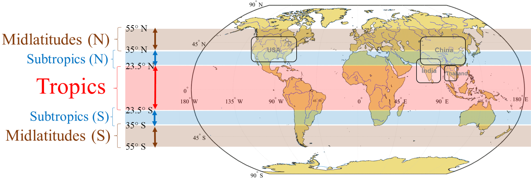
Figure 1 Spatial segmentation to assign the global flood events (1985 to 2015) into different latitudinal belts: midlatitudes (N): 35–55^∘ N; subtropics (N): 23.5–35^∘ N; tropics: 23.5^∘ S–23.5^∘ N; subtropics (S): 23.5–35^∘ S; and midlatitudes (S): 35–55^∘ S; (N) and (S) indicate Northern Hemisphere and Southern Hemisphere, respectively; the four rounded rectangles shows the United States of America (USA), China, India, and Thailand.

Next, for each latitudinal belt, the total number of floods per year (calendar year from 1 January to 31 December), the duration of these floods, and their location (name of country) are processed. This procedure is formulated as follows:

$$\begin{array}{ll}{\displaystyle }{F}_{\mathrm{C}}^{t,\mathrm{r}}=& {\displaystyle }\mathrm{total}\mathrm{number}\mathrm{of}\mathrm{flood}\mathrm{event}\left(\mathrm{s}\right)\mathrm{in}\mathrm{latitudinal}\mathrm{belt}r\\ \text{(1)}& {\displaystyle }& {\displaystyle }\mathrm{and}\mathrm{year}t\left[\mathrm{count}\right(\mathrm{s}\left)\right],\end{array}$$

$$\begin{array}{ll}{\displaystyle }{\mathit{F}}_{\mathrm{D}}^{t,\mathrm{r}}=& {\displaystyle }\mathrm{duration}\left(\mathrm{s}\right)\mathrm{of}\mathrm{flood}\mathrm{event}\left(\mathrm{s}\right)\mathrm{in}\mathrm{latitudinal}\mathrm{belt}r\\ \text{(2)}& {\displaystyle }& {\displaystyle }\mathrm{and}\mathrm{year}t\left[\mathrm{day}\right(\mathrm{s}\left)\right],\end{array}$$

$$\begin{array}{ll}{\displaystyle }{\mathit{F}}_{\mathrm{L}}^{t,\mathrm{r}}=& {\displaystyle }\mathrm{location}\left(\mathrm{s}\right)\mathrm{of}\mathrm{flood}\mathrm{event}\left(\mathrm{s}\right)\mathrm{in}\mathrm{latitudinal}\mathrm{belt}r\\ \text{(3)}& {\displaystyle }& {\displaystyle }\mathrm{and}\mathrm{year}t\left[\mathrm{name}\mathrm{of}\mathrm{country}\right(\mathrm{ies}\left)\right],\end{array}$$

where F_C indicates the flood counts (frequency), and F_D and F_L denote the vectors of flood duration and flood location for each of these flood events, respectively. The superscripts r and t denote the latitudinal belt (r = {global, tropics, midlatitudes (N and S), subtropics (N and S)}) and year (t = {1985, 1986, …, 2015}).

In addition, the number of floods in each latitudinal belt are also categorized in terms of their duration. We denote the event as a short-duration flood $F_{{\mathrm{C}}_{\mathrm{S}}}^{t,\mathrm{r}}$ if the duration is between 1 and 7 days, moderate-duration flood $F_{{\mathrm{C}}_{\mathrm{M}}}^{t,\mathrm{r}}$ if the duration is between 8 and 20 days, and as a long-duration flood $F_{{\mathrm{C}}_{\mathrm{L}}}^{t,\mathrm{r}}$ if the duration is greater than or equal to 21 days. These categories are also consistent with the DFO's flood classification (Brakenridge, 2016). The subscripts “S”, “M”, and “L” stand for short-, moderate-, and long-duration flood events, respectively.

2.3 Atmospheric teleconnections and climate indices

We used large-scale ocean–atmospheric teleconnections to investigate the extent to which the trends in the floods can be related to natural variability (Enfield et al., 2001; Ward et al., 2016) in the climate–atmospheric system. Since the climate system has as quasi-periodic nature that often manifests as wet and dry regimes, it is important to understand whether the trends, if observed, can be attributed to these natural oscillations. Hence, we used the El Niño–Southern Oscillation (ENSO), Pacific Decadal Oscillation (PDO), North Atlantic Oscillation (NAO), and Atlantic Multidecadal Oscillation (AMO) as proxies for interannual, decadal, and multidecadal climate variability.

We obtained 31 years (1985–2015) of ENSO data (aggregated based on the monthly anomalies of Niño 3.4) from the HadISST1 dataset (Rayner et al., 2003). Monthly AMO and PDO anomalies are obtained from the NOAA/Earth System Research Laboratory at http://www.esrl.noaa.gov/psd/data/climateindices/list (last access: 1 March 2016) (Zhang et al., 1997), and then averaged to yearly time series from 1985 to 2015. Similarly, the monthly NAO indices are obtained from the NOAA/National Weather Service, Climate Prediction Center at http://www.cpc.ncep.noaa.gov/products/monitoring_and_data/ (last access: 1 March 2016) (Barnston and Livezey, 1987; Hurrell and Van Loon, 1997) and averaged to yearly time series.

2.4 Calculating resistant metrics from the distribution of flood duration

In addition to the frequency of the floods ($F_{\mathrm{C}}^{t,\mathrm{r}}$), we calculate a set of “resistant measures” to evaluate the existence of any significant monotonic time trend in the probability distribution of flood duration. Four moment indicators are selected because of their scale-invariant characteristics suitable for such asymmetric distributions. These metrics include the median, median absolute deviation (MAD), resistant skewness, and the 90th percentile of the distribution of flood durations in each year. Each of these metrics is computed as a time series of 31 years (1985–2015) for each of the six spatial scales (i.e., global, tropics, midlatitudes – N, midlatitudes – S, subtropics – N, subtropics – S). It is straightforward to calculate the median and 90th percentile from the distribution of flood duration each year. We explain the formulation and the properties of the other two metrics here.

Table 1 Proposed hypotheses and evaluation approach.

2.4.1 Median absolute deviation (MAD) of flood durations

We calculate the MAD of flood duration as an indicator of the deviation from the central tendency. The MAD is a robust measure to quantify the within-year variation in flood duration. It is a good measure of scale for distributions with heavier tails (Sachs, 2012). It is also resistant to the influence of outliers (Hampel, 1974). Contrary to the standard deviation (SD) – which is affected by non-normality of the probability distribution and extremely high or low values – the presence of outliers does not influence the MAD value (Leys et al., 2013). However, the interpretation of MAD is similar to SD, as it measures the deviation from the average flood duration. MAD is computed as follows:

$$\begin{array}{}\text{(4)}& {\displaystyle }{\displaystyle }{\mathit{F}}_{{\mathrm{D}}_{\mathrm{MAD}}}^{t,\mathrm{r}}=\mathrm{median}\left(\left|{\mathit{F}}_{\mathrm{D}}^{t,\mathrm{r}}-F_{{\mathrm{D}}_{\mathrm{Median}}}^{t,\mathrm{r}}\right|\right),\end{array}$$

where “t”, “r”, and ${\mathit{F}}_{\mathrm{D}}^{t,\mathrm{r}}$ are the same variables defined in Eq. (2) and $F_{{\mathrm{D}}_{\mathrm{Median}}}^{t,\mathrm{r}}$ refers to the median of distribution of flood duration.

2.4.2 Resistant skewness of flood durations

The presence of outliers amongst the variables will generate a large and possibly misleading measure of skewness (Helsel and Hirsch, 1992). Instead, the resistant skewness is a more robust measure for capturing the asymmetrical or symmetrical properties in the data. It is estimated using the following equation:

$$\begin{array}{}\text{(5)}& {\displaystyle }{\displaystyle }{F}_{{\mathrm{D}}_{\mathrm{rSkewness}}}^{t,\mathrm{r}}={\displaystyle \frac{\left(F_{{\mathrm{D}}_{\mathrm{0.75}}}^{t,\mathrm{r}}-F_{{\mathrm{D}}_{\mathrm{Median}}}^{t,\mathrm{r}}\right)-\left(F_{{\mathrm{D}}_{\mathrm{Median}}}^{t,\mathrm{r}}-F_{{\mathrm{D}}_{\mathrm{0.25}}}^{t,\mathrm{r}}\right)}{\left(F_{{\mathrm{D}}_{\mathrm{0.75}}}^{t,\mathrm{r}}-F_{{\mathrm{D}}_{\mathrm{0.25}}}^{t,\mathrm{r}}\right)}},\end{array}$$

where $F_{{\mathrm{D}}_{\mathrm{rSkewness}}}^{t,\mathrm{r}}$ is the resistant skewness of flood duration, “r” and “t” are the same variables previously given in Eq. (2), and $F_{{\mathrm{D}}_{\mathrm{0.25}}}^{t,\mathrm{r}}$ and $F_{{\mathrm{D}}_{\mathrm{0.75}}}^{t,\mathrm{r}}$ refer to the 25th and 75th percentiles of flood durations for each year for the specified latitudinal belt.

Note that the sample sizes (number of floods) may be different for different years. For instance, the total number of floods in 1985 at the global scale is 69. We compute the median, MAD, skewness, and the 90th percentile of the duration for these 69 events. Similarly, the total number of floods in 2015 at the global scale is 101, and we compute the median, MAD, skewness, and the 90th percentile for these 101 events. After obtaining the time series of these metrics, we then investigate for monotonic time trends.

2.5 Country-scale flood frequency and flood damage statistics

For a specific country, we calculate the relative flood frequency of short, moderate, and long durations with respect to the total flood events occurring in that country. This can help us identify what flood duration class has occurred more frequently from 1985 to 2015 in that country. Correspondingly, the reported flood damage for that event has also been noted along with its relative damage in reference to the total flood damages in that country from 1985 to 2015.

In order to investigate the association between flood duration and damage at the country scale, we present a linear model for flood damage (F_damage) as a function of flood duration (F_D) in the log space as follows:

$$\begin{array}{}\text{(6)}& {\displaystyle }{\displaystyle }{F}_{\mathrm{damage}}=\mathit{\alpha }{F}_{\mathrm{D}}^{\mathit{\beta }}⟹\log \left(F_{\mathrm{damage}}\right)=\log \left(\mathit{\alpha }\right)+\mathit{\beta }\log \left(F_{\mathrm{D}}\right),\end{array}$$

where α and β are the intercept and scaling exponents, respectively, of flood damage for a specific country. The parameter β in this formulation captures the change in flood damage due to changes in flood duration.

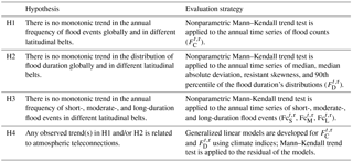
2.6 Hypotheses

Most of the global precipitation studies indicate that there is a recent increase in both the annual precipitation and extreme rainfall intensities (Solomon, 2007; Zhou et al., 2013). Consequently, our goal here is to investigate whether we see a significant trend in the frequency and duration of floods during the last 3 decades. Based on this, the main hypotheses (H1, H2, H3, and H4) and the evaluation procedure are presented in Table 1.

We begin our investigation with H1, the hypothesis that there is no monotonic trend in the annual frequency of the flood events. We test this hypothesis using the Mann–Kendall (MK) trend test (Mann, 1945). The MK test uses the ranks of the data and assumes no underlying probability distribution (Helsel and Hirsch, 1992). The test statistic is based on a pairwise comparison among the values and is independent of the distribution of the original series. The magnitude of the slope of the trend is estimated using the method of Sen, the median of the pairwise slopes among the elements of the series (Sen, 1968). Ties in the data are adjusted using an assumption that the number of ties is equal to an even number of positive and negative differences (Burkey, 2006). Statistical significance is evaluated at the 5 % significance level, the probability of incorrectly rejecting the null hypothesis.

In hypothesis H2, we explore whether there is a change in the probability distribution of the flood duration over time. We test this hypothesis by applying the MK trend test on the three resistance moments (median, MAD, and skewness) and the 90th percentile (extreme flood duration) of the annual distribution of the flood duration. H3 is intended to investigate the changes in the patterns of flood frequencies for each category: short-, moderate-, and long-duration floods. Lastly, in H4, we investigate the potential large-scale atmospheric teleconnections to which the observed trend(s) in H1 and H2 can be related by using a GLM framework.

2.7 The generalized linear model (GLM) framework

Our hypothesis (H4) is that the detected time trend is due to cyclical climate influences (i.e., oscillatory behavior) associated with the large-scale ocean–atmospheric interactions. Hence, for all the cases in which the null hypothesis of no trend is rejected, we attempted to understand whether the trend relates to large-scale climate oscillations. For this purpose, we employed a GLM framework on the time series of the above-developed metrics with ENSO, AMO, PDO, and NAO as covariates. GLMs are the mathematical extension of classical linear regression models to include a broad class of model assumptions such as linear, Poisson, exponential, log-linear, and so on with specified link functions (Chandler and Wheater, 2002; McCullagh, 1984; Yang et al., 2005). For all the spatial scales at which we see a statistically significant trend, a GLM is fit to the time series (1985–2015) of F_C, $F_{{\mathrm{D}}_{\mathrm{Median}}}$, and $F_{{\mathrm{D}}_{\mathrm{90}}}$ with climate covariates.

$$\begin{array}{}\text{(7)}& {\displaystyle }& {\displaystyle }{F}_{\mathrm{C}}=a+b_{\mathrm{1}}\mathrm{ENSO}+b_{\mathrm{2}}\mathrm{AMO}+b_{\mathrm{3}}\mathrm{PDO}+b_{\mathrm{4}}\mathrm{NAO},\text{(8)}& {\displaystyle }& {\displaystyle }{F}_{{\mathrm{D}}_{\mathrm{Median}}}=a+b_{\mathrm{1}}\mathrm{ENSO}+b_{\mathrm{2}}\mathrm{AMO}+b_{\mathrm{3}}\mathrm{PDO}+b_{\mathrm{4}}\mathrm{NAO},\text{(9)}& {\displaystyle }& {\displaystyle }{F}_{{\mathrm{D}}_{\mathrm{90}}}=a+b_{\mathrm{1}}\mathrm{ENSO}+b_{\mathrm{2}}\mathrm{AMO}+b_{\mathrm{3}}\mathrm{PDO}+b_{\mathrm{4}}\mathrm{NAO},\end{array}$$

where a, b₁, b₂, b₃, and b₄ are the GLM's coefficients (parameters). We then select the best model using the forward and backward stepwise regression and obtain the residuals of the best model in each case. The residuals represent the values for F_C, $F_{{\mathrm{D}}_{\mathrm{Median}}}$, and $F_{{\mathrm{D}}_{\mathrm{90}}}$ after adjusting for the influence of exogenous variables. In other words, they reveal the variability beyond what could be attributed to exogenous climate factors. The analysis of the time trends in the residuals will help discern any unexplained trend after accounting for background variability due to the climatic modulation (e.g., Armal et al., 2017; Merz et al., 2012). The models are fit using the “stepwiseglm” toolbox in MATLAB 2017a (McCullagh, 1984) that uses the forward and backward regression algorithm. We used the deviance information criterion for the best model selection among a finite set of models. Results from the models are presented in Sect. 4 in which we discuss the associations.

3 Results

3.1 Addressing H1: trends in the annual frequency of flood events

The MK test (Eqs. A1–A3) is applied to each time series of F_C (i.e., global, tropics, midlatitudes – N, midlatitudes – S, subtropics – N, and subtropics – S) for the detection of monotonic trends. Figure 2 presents the time series of F_C for the global scale and the five latitudinal belts. A solid LOESS (local regression) curve is shown if the trend is significant. Alternately, a dashed LOESS curve is shown for the time series that do not exhibit a statistically significant trend. The detailed statistics derived from the trend analysis are given in Table 2.

A total of 4311 flood events occurred during last 3 decades worldwide. The results of the MK test on the annual frequency of global floods indicate that there is a statistically significant monotonic trend with τ (Kendall correlation coefficient between F_C and time) and β (robust Sen slope) values of 0.26 and 2.12, respectively. A total of 2020 events (out of the 4311 floods) occurred in the tropics. The hypothesis that there is no trend in the frequency of floods in the tropics is rejected. This is also the case for both the subtropics (S) and midlatitudes (S). However, while we see an uptrend in the number of floods in the midlatitudes (S) post-2000, we urge caution in interpreting this trend as zeros dominate the time series. Finally, for both the subtropics (N) and midlatitudes (N), the hypothesis that there is no trend in the annual frequency of floods cannot be rejected at the 5 % significance level.

• H1. There is a statistically significant increase in the frequency of floods at the global scale, and over the tropics, subtropics (S), and midlatitudes (S). The temporal pattern of the data for global floods resembles that of the tropics.

Table 2 Summary of trend analysis (Mann–Kendall test with a significance level α = 0.05) on the frequency of flood events at the global scale and the five latitudinal belts.

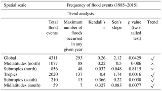
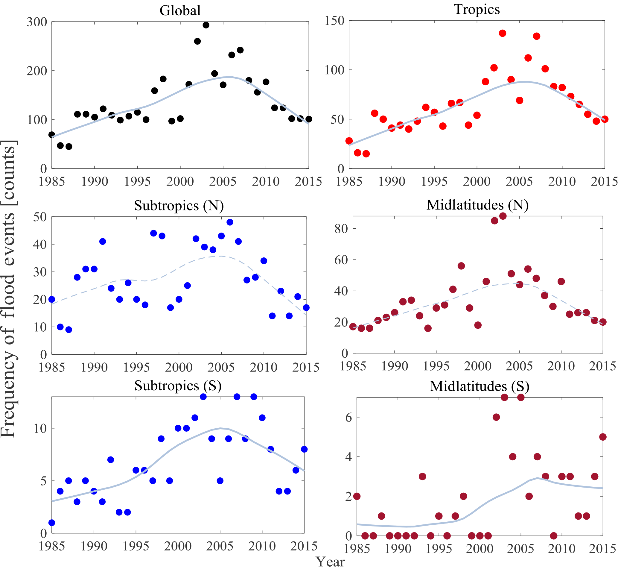
Figure 2 Frequency of flood events at the global scale and the latitudinal scales (i.e., tropics, subtropics – N, subtropics – S, midlatitudes – N, and midlatitudes – S); a LOESS curve fitting is shown (solid line) for the time series in which a significant trend in the number of flood events is observed (Mann–Kendall test with significance level α = 0.05). A dashed line indicates the LOESS curve for the regions with insignificant trends.

3.2 Addressing H2: trends in the distribution of flood duration

The MK trend tests are performed on the time series of the median, MAD, resistant skewness, and the 90th percentile of the flood duration. The following four subsections elaborate the results for each metric.

Table 3 Same as Table 2 but for the median of flood durations.

Figure 3 Same as Fig. 2 but for the median of flood durations.

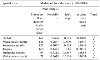
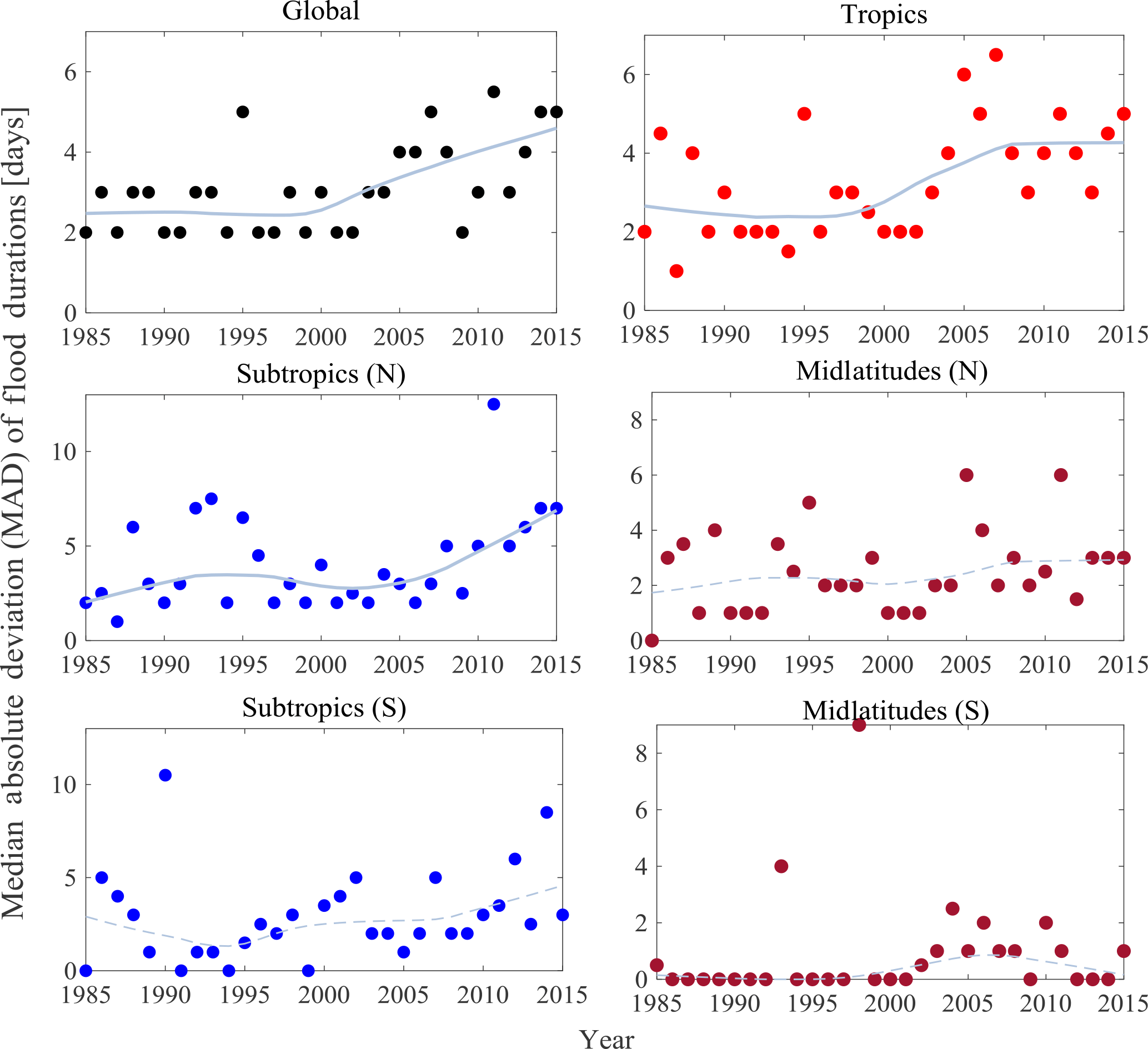
3.2.1 Trends in the median of flood durations

From Fig. 3, we can see that there is a statistically significant monotonic trend in the median of the flood duration at the global scale and all sub-spatial scales. We see that the median of the flood duration at the global scale has increased steadily from 4 days in the year 1985 to 10 days in the year 2015, indicating that the median flood duration changed to moderate duration in 2015 from short duration in 1985. In other words, it shifted one class from being less than 1 week to between 1 week and 3 weeks. Similar shifts can be observed in the tropics and the subtropics. In Table 3, we present the statistics of the tests. As in the case of the frequency of floods, we urge caution in interpreting the trends seen in the midlatitudes (S) due to the presence of zeros.

Figure 4 Same as Fig. 2 but for median absolute deviation (MAD) of flood durations.

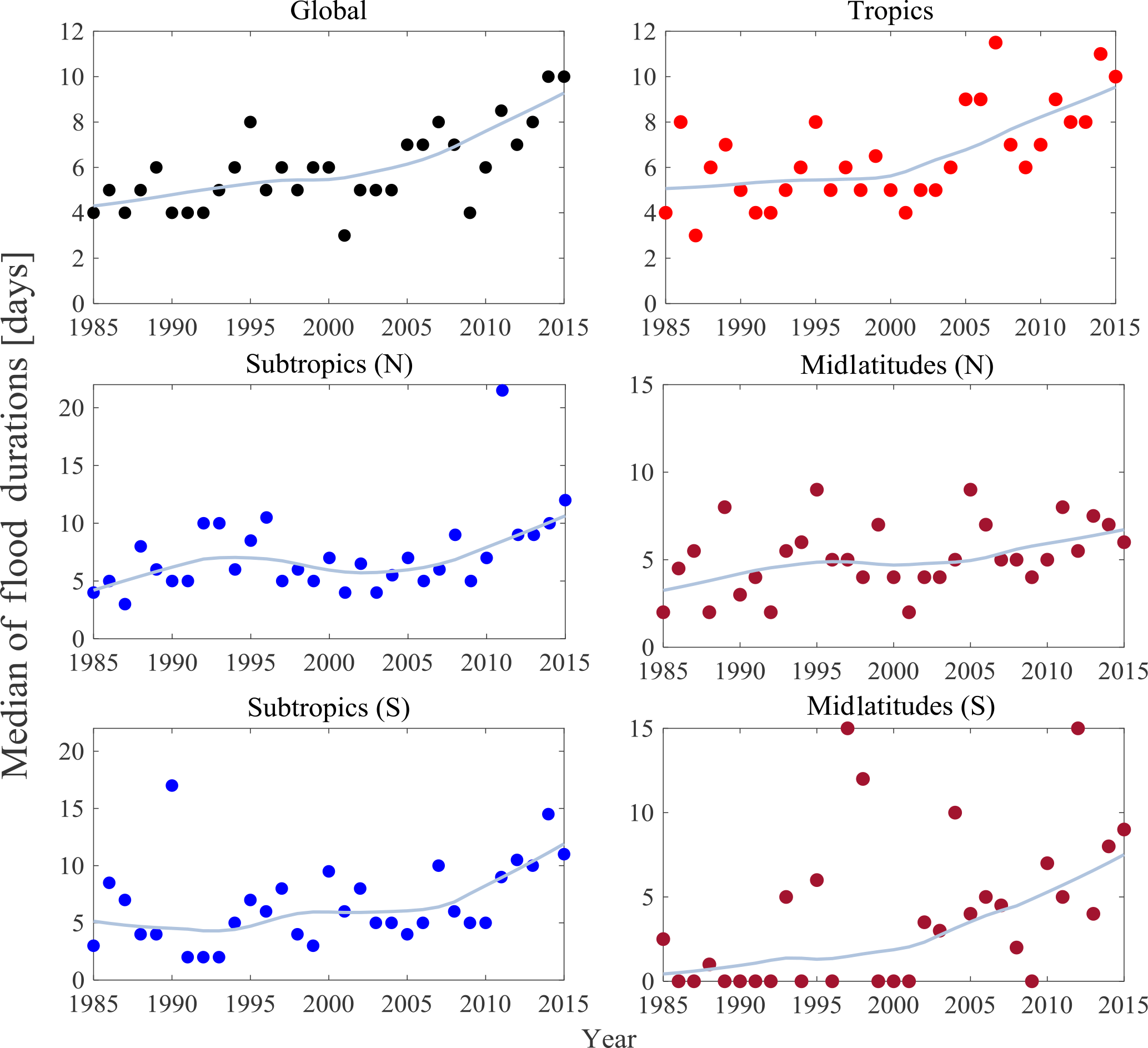
3.2.2 Trends in the median absolute deviation (MAD) of flood durations

The MK trend test is performed on the MAD of flood duration (Eq. 4) at the different global and latitudinal scales and presented in Fig. 4 and Table 4.

The output statistics show that there is a significant increasing trend in MAD at the global scale, and in the tropics and subtropics (N). It is interesting to note that the MAD has essentially remained constant, around 2–3 days from 1985 to 2000, and has increased since to around 5 days in 2015, indicating increased variability in flood durations within years in these belts recently. There is no significant change in the variability in the midlatitudes (N and S) and subtropics (S).

Table 4 Same as Table 2 but for the median absolute deviation (MAD) of flood durations.

Figure 5 Same as Fig. 2 but for the resistant skewness of flood durations.

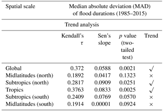
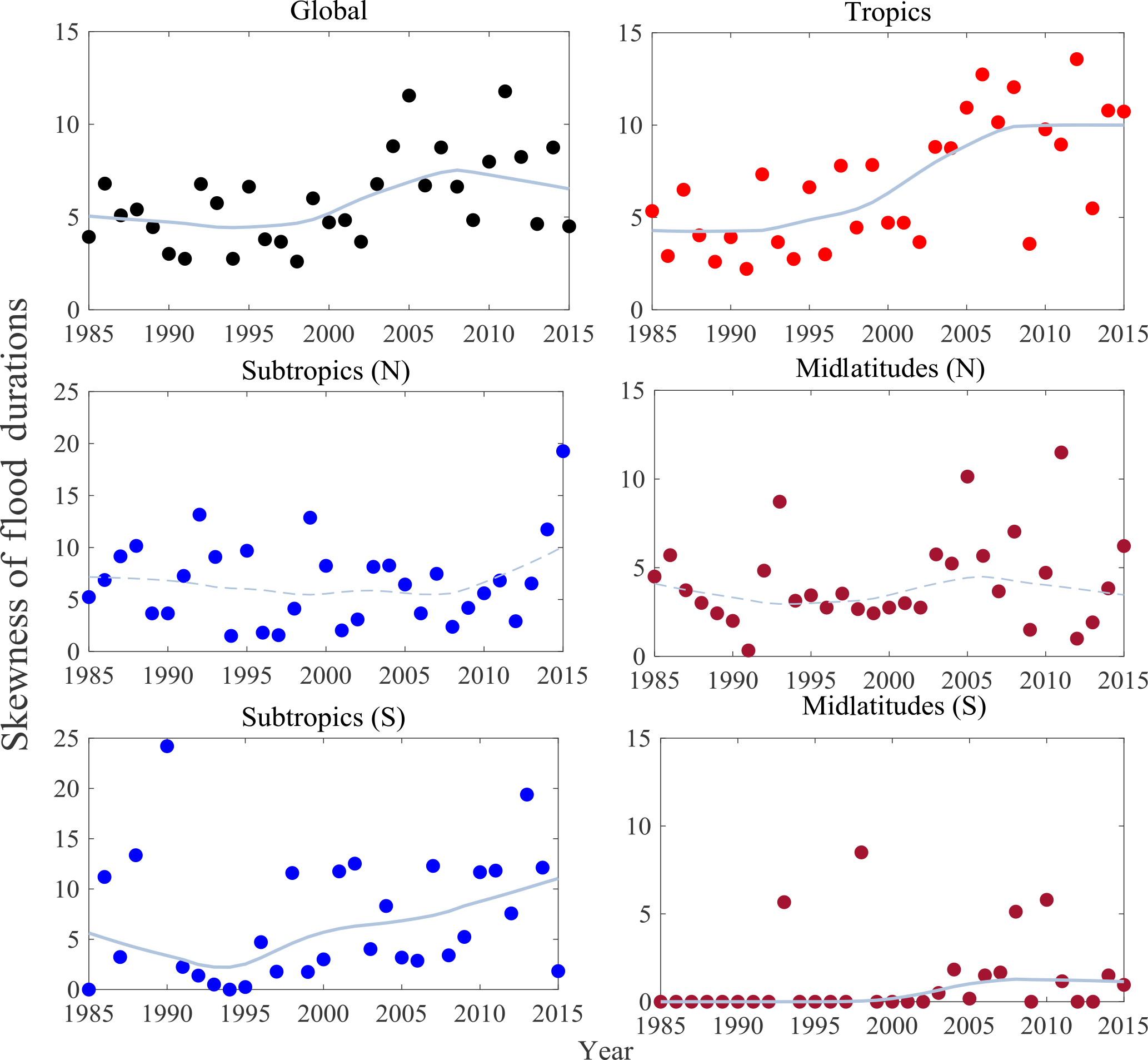
Table 5 Same as Table 2 but for the resistant skewness of flood duration distributions.

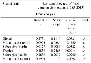
3.2.3 Trends in the resistant skewness of flood duration

The resistant skewness of flood duration is calculated for each time series using Eq. (5) and presented in Fig. 5. As before, the MK trend test is applied to these time series. A statistically significant trend in the skewness is observed at the global scale and tropical and subtropical (S) latitudes. Similar to Tables 2–4, in Table 5 we present the test statistics. We observe that the yearly asymmetrical/symmetrical behavior of the distribution of flood durations has considerably changed during the last 3 decades (from 5 to 8 approximately), with a more significant tendency towards high skewness. This change towards a right-skewed-type distribution of flood durations (e.g., from 5 to 8) can be due to the increase in occurrence of moderate- or longer-duration floods. Conversely, there is no significant trend in the skewness of flood duration in the subtropics (N) and midlatitudes (N) at the 5 % significance level.

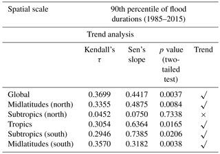
3.2.4 Trends in the 90th percentile of flood durations

Finally, we test for monotonic trend in the extreme values (expressed here as the 90th percentile) of flood duration. This measure serves as a surrogate for extremely long-duration flood events each year. By definition, the 90th percentile of the flood duration ($F_{{\mathrm{D}}_{\mathrm{90}}}^{t,\mathrm{r}}$) is the value which is exceeded by only 10 % of the events in that year (year “t”) in the latitudinal belt “r”. Consequently, a value as large as this indicates the long-duration extent of the flood. Figure 6 and Table 6 present the summary of MK analysis on the 90th percentile of flood duration.

The extreme duration of floods has substantially changed over the last 3 decades at the global scale, tropics, midlatitudes (N and S), and subtropics (S), as presented in Table 6. The null hypothesis that there is no monotonic trend in the tails is rejected in all regions, except the subtropics (N). Furthermore, we find that the extreme values of the long-duration flood events are more than 30 days in the recent decade, whereas they were less than 20 days in the 1980s and 1990s. The increase was monotonic.

Figure 6 Same as Fig. 2 but for the 90th percentile of flood durations.

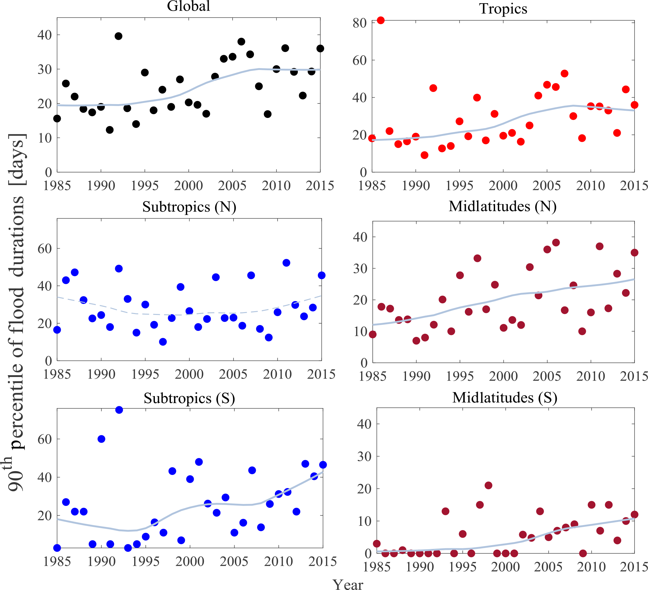
Table 6 Same as Table 2 but for the 90th percentile of flood duration distributions.

The highlights of trend analyses presented in Figs. 3 to 6 and Tables 3 to 6 are outlined below:

• H2. The median of flood duration has increased at the global scale and all sub-spatial scales. There is also an increasing monotonic trend in the MAD (within the year variability) of flood duration across the global, tropical, and subtropical (N) spatial scales. We also see an increase in the resistant skewness of flood duration around the globe, tropics, subtropics (S), and midlatitudes (S). For the extreme flood durations (i.e., 90th percentile), we see an increasing trend in all spatial scales except the subtropics (N) over the past 3 decades. Due to the presence of a significant number of zeros in the statistics of the floods, we urge caution in interpreting the trends seen in the midlatitudes (S).

3.3 Addressing H3: trends in the frequency of short-, moderate-, and long-duration floods

Given that we find statistically significant trends in the tails of the distribution (90th percentile of the duration of floods), we were interested in exploring whether there would be a trend in the frequency of the long-duration floods as well. To investigate this, we performed the MK test on the frequency of long-duration floods ($F_{{\mathrm{C}}_{\mathrm{L}}}$) for the tropics, subtropics, and midlatitudes. We also performed these tests on short-duration flood frequency ($F_{{\mathrm{C}}_{\mathrm{S}}}$) and moderate-duration flood frequency ($F_{{\mathrm{C}}_{\mathrm{M}}}$). We present these results in Table 7.

Table 7 Summary of trend analysis (Mann–Kendall test with a significance level α = 0.05) on three flood classes: short, moderate, and long durations of flood events over five latitudinal belts.

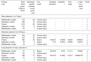
As it can be seen from Table 7, there is no monotonic trend in the frequency of short-duration floods occurring across all the spatial scales, indicating that the number of short-duration floods has not changed significantly over the last 3 decades worldwide. However, this phenomenon is not true for moderate- and long-duration floods. In fact, the frequency of both moderate- and long-duration floods has increased in the tropics. There is also an increasing trend in moderate-duration floods in the subtropics (S) and long-duration floods in the midlatitudes (N). These findings are consistent with the results from H2, where we see a trend in the skewness and the tails of floods in these belts. An increase in the frequency of moderate- and long-duration floods will result in a shift of the quantile of flood duration distribution, thereby changing the skewness and the tails.

For the long-duration flood events in the tropics, the total number of events has increased from 60 before 2000 to 249 after 2000. Similarly, the total number of events in the midlatitudes has increased from 27 to 70 post-2000. In other words, there are 4 times more long-duration floods that occurred during the most recent 15 years than before the year 2000. The increase across the midlatitudes (N) is around 2.5 times pre- and post-2000.

• H3. In summary, frequency of moderate- and long-duration flood classes has changed recently, but remains unchanged for the short-duration floods in all the latitudinal belts. The annual frequencies of moderate- and long-duration flood events have increased across the tropics and midlatitudes (N) (on the scale of 4 and 2.5 events per year, respectively) over last 3 decades.

3.4 Country-scale vulnerability analysis to short-, moderate-, and long-duration flood events

There were 4311 flood events that occurred from 1985 to 2015 around the world. According to Tables 2 and 7, globally, the total number of short-, moderate-, and long-duration flood events was 2508 (≈ 59 %), 1151 (≈ 27 %), and 560 (≈ 13 %), respectively. In addition to the aggregate analyses at the latitudinal level, we also explored the country-scale vulnerability to short-, moderate-, and long-duration floods. We interpret vulnerability as the expected value of the damage due to floods, i.e., the severity of the consequence of the floods (Hashimoto et al., 1982; Holling, 1978).

For this purpose, we first excluded countries which had less than 31 flood events to ensure that we investigate only those counties that have experienced at least one flood per year on average. This screening resulted in 28 countries with a minimum of 31 flood events during the last 3 decades. These 28 flood-prone countries are sorted as follows: the United States (388 events), China (344 events), India (226 events), Indonesia (190 events), Philippines (181 events), Australia (121 events), Vietnam (107 events), Brazil (96 events), Bangladesh (88 events), Mexico (80 events), Iran (77 events), Afghanistan (74 events), Russia (69 events), Thailand (66 events), Pakistan (66 events), Nigeria (57 events), Malaysia (54 events), Kenya (49 events), Canada (48 events), Colombia (44 events), Peru (43 events), Turkey (41 events), Nepal (40 events), France (40 events), Romania (38 events), Ethiopia (35 events), Somalia (34 events), and New Zealand (31 events).

Then, the fraction of flood frequencies for each country and duration class – short, moderate, and long – is calculated. Figure 7a presents these fractions for the 28 countries using the ternary plot. For 23 of these countries, we have the data on the damages due to the floods. We computed the expected value of the damages for each country and plotted the fractional damage due to short-, moderate-, and long-duration floods as the second ternary plot in Fig. 7b. The color bars indicate the total number of events (Fig. 7a) and the total flood damage (Fig. 7b). In each plot, the location of the country shows the relative fraction of short-, moderate-, and long-duration flood frequency and damage. For example, in Fig. 7a, the United States is identified as a red circle in the top corner with > 60 % of floods being short duration, between 20 and 30 % of the floods being moderate, and only < 10 % of them being long-duration floods. However, in terms of the vulnerability to floods (Fig. 7b), the United States is located in the bottom right corner of the triangle, indicating that most of the vulnerability is due to low-probability long-duration floods. Similar observations can be made for Vietnam, Mexico, Indonesia, Australia, and Malaysia, to name a few. These countries have a very low probability of long-duration floods, but the consequence of these floods is the most important in terms of the vulnerability. It is also noteworthy to emphasize that for most of the countries, the overall damage is dominated by the damage due to moderate- and long-duration floods. This can be seen from the fact that many of the countries are found in the bottom left and right corners of the ternary plot.

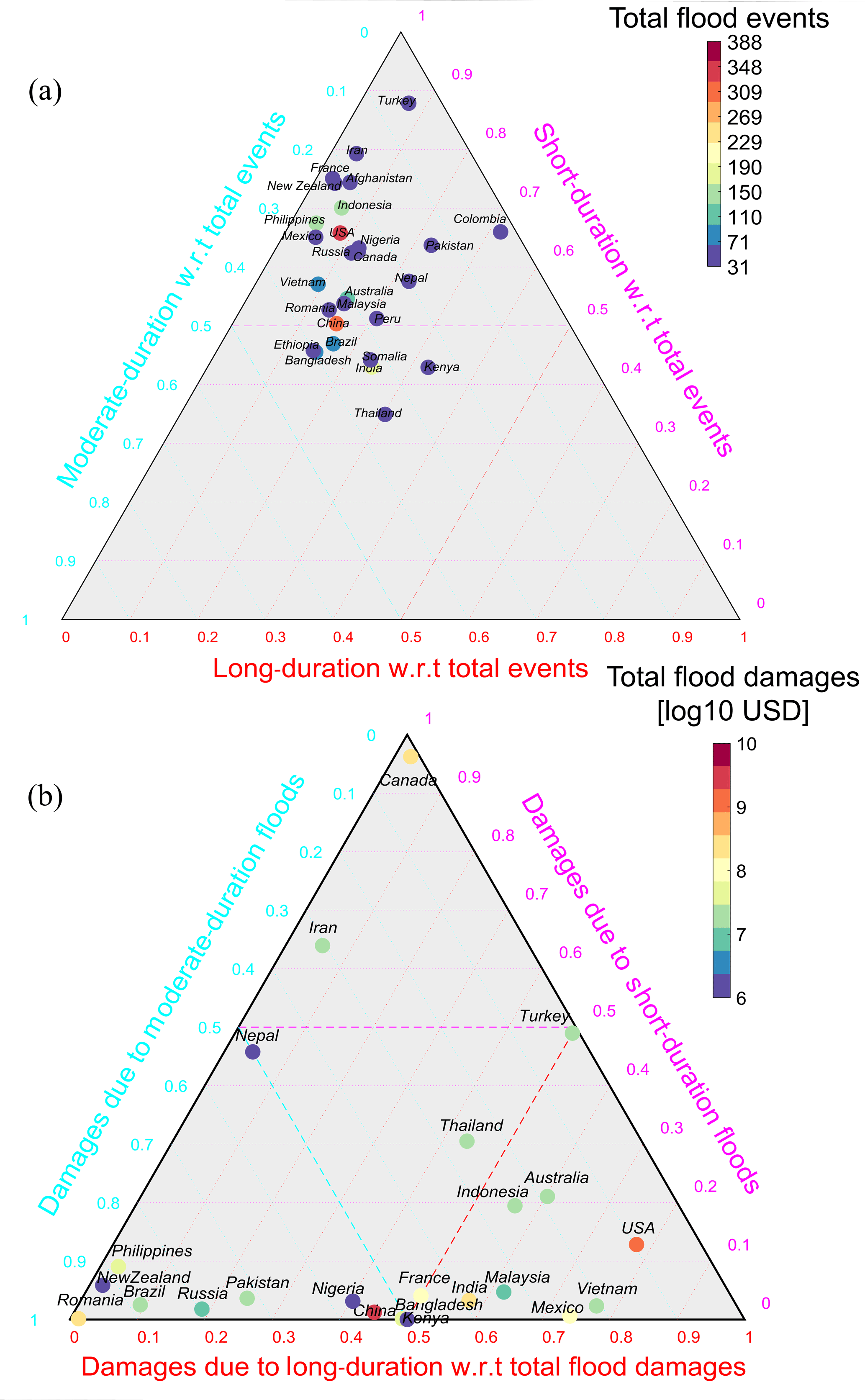
Figure 7 (a) Relative frequency of short- (less than 7 days), moderate- (8 to 20 days), and long-duration (21 days and above) floods for the countries with at least 31 events from 1985 to 2015; (b) relative flood damages due to short-, moderate-, and long-duration floods with respect to total flood damages for the countries with at least 31 events from 1985 to 2015 (except Colombia, Peru, Ethiopia, Somalia, and Afghanistan due to lack of data).

To further understand the relation between flood duration and flood damage, we fit log-linear models given in Eq. 6 for four selected countries: the United States, Thailand, India, and China. The results of the log-linear models for these four countries are shown in Fig. 8a. These countries are selected because they have the highest number of long-duration floods among all countries (Fig. 8b). Parameter β is the scaling exponent of the damages to the flood duration. Note that the scaling exponent is similar for the United States (0.89) and China (1.03) while India (0.23) and Thailand (0.56) have much smaller exponents. In total, 226 flood events occurred across India, of which around 43, 32, and 25 % of them were short-, moderate-, and long-duration events, respectively. In the United States, short-, moderate-, and long-duration flood events account for 66, 26, and 8 % of 388 flood events that occurred in the last 3 decades. However, the fraction of long-duration flood events is much higher for Thailand (30 % of total flood events). In China, around half of the flood events were related to the moderate- or long-duration flood classes (34 and 16 %, respectively). This opens up new questions about whether there are consistent relations like this across the globe and how different these scaling exponents would be. We do not pursue them as part of this investigation, however, in the spirit of examining flood duration and damages, in Fig. 8b and c, we present the data on flood duration and flood damage ranked for various other countries.

According to the DFO flood data from 1985 to 2015, the ranking results show that the frequency of short-duration floods for the United States, China, India, and the Philippines is respectively 255, 173, 133, and 122. For moderate-duration floods, the countries of China, the United States, India, and the Philippines have experienced 118, 101, 74, and 52 flood events, respectively. The long duration floods were seen mostly in India (55 events), China (53 events), the United States (32 events), and Thailand (20 events) from 1985 to the end of 2015. It should be noted that here we only presented the top 21 countries in each category.

As discussed in this section, the consequences of floods of different durations should be paid attention to, as this plays a big role in designing appropriate flood-proofing infrastructure and developing early warning systems and flood insurance payout structures. The relation between the duration of floods and the induced damages, and how they might vary across different countries, was also investigated here.

4 Discussion

The trends in the frequency and the distribution of the floods (prominent in long-duration floods) may be related to several causes ranging from measurement uncertainty in the DFO flood data, climate and atmospheric teleconnections, and socioeconomic contributions such as the increased exposure to the flood events. We attempt to explain these possibilities in the following two sections.

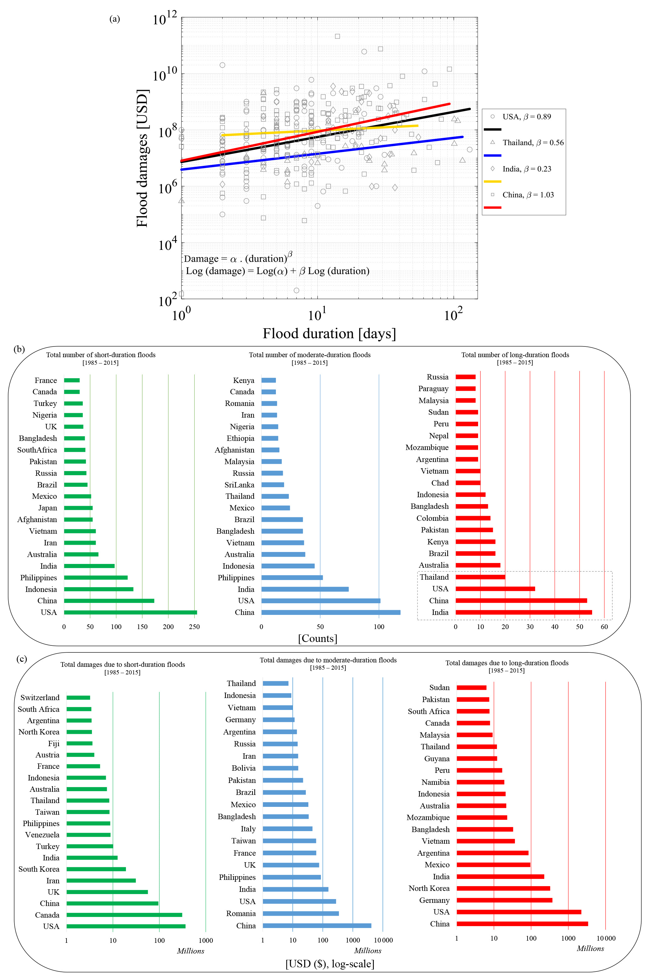
Figure 8 (a) Covariation of flood duration with the corresponding flood damages for the top four countries with the maximum number of long-duration flood events (i.e., India, China, the United States, and Thailand), (b) total number of short- (less than 7 days), moderate- (8 to 20 days), and long-duration (21 days and above) floods, and (c) total damages due to short-, moderate-, and long-duration floods. These countries are the top 21 countries, which are ranked based on the frequency of each flood duration category and corresponding flood damages using the DFO flood data from 1985 to 2015.

4.1 What are the uncertainties in DFO flood archive data, and/or has the exposure to the flood events changed?

The flood archive data provided by the DFO have been collected using different methods of observation and validation since 1985 (see the summary of the methods in Brakenridge et al., 2005). In addition, there are more flood warning systems and facilities, transmitting instruments, reporting networks, and communications today at different levels of social and governmental divisions that the DFO is using to provide more comprehensive flood information. They have improved their flood detection methods by including the MODIS products since 1999. MODIS products contain surface inundation information based on vertically and horizontally polarized backscatter acquired remotely from the radiance changes among water-, land-, and vegetation-covered surfaces (Brakenridge et al., 2007). We acknowledge that there could be some uncertainties as a result of this since surface may also be interpreted as water in the presence of clouds, cloud shadows, and mountainous terrain (Brakenridge et al., 1998). Further, inclusion of this improved technology will result in better monitoring of floods. This improvement is likely a potential driver of trend in the flood duration. In our analysis of H3, we find that there is no significant trend in the frequency of short-duration events across all latitudinal scales (Table 7), but a significant trend can be seen across the tropics for moderate- and long-duration flood events. The introduction of improved satellite products would have increased the chances of detecting more short-duration floods (small events) along with providing better resolution for longer floods. We think that it is not possible to see the systematic contributions of such products into only one specified type(s) of flood duration.

To validate the DFO's flood statistics, we have corroborated the DFO floods with the available in situ streamflow observations from the GRDC (The Global Runoff Data Centre, 56068 Koblenz, Germany, 2013, http://grdc.bafg.de, last access: 1 December 2017). Among the stations that had matching time periods and locations, we found that a high percent of stations (≈ 90 %) have very few errors (i.e., less than 7 days) when their flood durations were compared. The results demonstrate that the recorded flood information in the DFO appears to be reliable with respect to the GRDC river discharge measurements (see more details in Appendix B). However, we did identify a reporting bias in the start and end dates of the floods where the events with no reported flood beginning date are assumed to start in the middle of the month. Some biases were also identified for days 1, 5, 10, 15, 20, and 25, which had an increased number of flood counts. These biases will potentially lead to estimation uncertainties in the trend model. We believe that interpretation at the global level will remain robust due to the effect of averaging and large numbers; at the local level interpretation needs more attention to such reporting details.

While understanding such uncertainties is essential, especially while interpreting trends in limited data, it is also documented in the literature that there has been an increased exposure to floods in recent times. The number of people, residential and industrial properties, and assets exposed to the flood events has drastically increased (Bouwer, 2011; Jongman et al., 2012; Kundzewicz et al., 2014). The type of vulnerability to flood risk is mostly connected to development of the country and its land use and environmental management (Peduzzi et al., 2009). Recent studies by Di Baldassarre et al. (2010) and Vogel et al. (2011) in Africa and the United States, respectively, showed that there had been a considerable change in the flood frequency and magnitude in regions which have undergone intense urbanization.

While exposure of people to floods is the main concern in developing countries, exposure of assets and properties to floods is the vital concern for the developed countries (Jongman et al., 2012). Recently, much residential and industrial infrastructure has moved to the flat and cheap lands of floodplains (Peduzzi et al., 2011). The nature of geomorphological features of land has been modified to embrace these new developments. Hirabayashi et al. (2013) and Stevens et al. (2016) have recently indicated that the increase in the reporting of floods can be linked to the rise in the land use development in the floodplains.

4.2 Can the trends be related to natural variability in the climate and atmospheric systems?

The frequency of heavy precipitation events has increased at the global scale (Groisman et al., 2005; Liu and Zipser, 2015; Zhou et al., 2013). Using daily precipitation observations from the Global Historical Climatology Network (GHCN) dataset, Alexander et al. (2006) showed that the distributions of precipitation indices in the 1979–2003 period are significantly different from the 1901–1950 period with a tendency towards wetter conditions. Solomon (2007), in the fourth assessment report of the Intergovernmental Panel on Climate Change (IPCC), discussed that the annual precipitation intensity has increased over high latitudes during the period from 1901 to 2005, except the southwest of the United States, northwestern Mexico, and the Baja California Peninsula. This IPCC report also highlights the increasing contribution of extreme rainfall events to the total precipitation across Europe and the United States, which mostly occurred during the last 3 decades of the 20th century. Westra et al. (2013) tested 8326 land-based rainfall stations (with at least 30 years of record from 1900 to 2009) and found that the annual maximum daily precipitation has significantly increased for more than two-thirds of these stations at the global scale.

Theoretical studies also discussed the fact that mean global precipitation intensity increased by 1–3 % (conditional on available energy budgets) in proportion to the 1 ^∘C increasing rate of surface air temperature. Trenberth (1999), Trenberth et al. (2003), Trenberth (2011), Schiermeier (2011), and Glur et al. (2013) among others have also argued that an increase in air temperature will increase the atmospheric water-holding capacity (Clausius–Clapyron relationship), leading to more intense and frequent precipitation events. Hence, fluctuating precipitation regimes would interrupt the current balances of components within the hydrological cycle and human activities (Dentener et al., 2006; Doherty et al., 2000). Consequently, a warmer and wetter atmosphere is likely to intensify the global water cycle that ultimately will result in more frequent and larger flood events.

The space–time distribution of these precipitation regimes is potentially related to the large-scale ocean–atmosphere circulations (Conticello et al., 2018; Lu and Hao, 2017; Najibi et al., 2017; Portmann et al., 2009; Yu et al., 2016) driven by the natural climatic variability (Trenberth et al., 2007; Zappa et al., 2015). Natural climate variability often causes periods of increasing extremes (flood-rich cycle) or decreasing extreme events (flood-poor cycle) depending on the phase of the climate (Armal et al., 2017; Blöschl et al., 2015; Cioffi et al., 2016; Hall et al., 2014; Merz et al., 2014).

Hence, in an effort to investigate any significant relationship between the observed trend in the flood data (characterized in H1 and H2) and the variability in the climate and atmospheric circulation patterns, we considered large-scale atmospheric teleconnections and climate indices (with quasi-periodicity in nature that can lead to wet–dry regimes) to explain the trend, i.e., to place the short-term trends within a longer climate variability context as argued by Merz et al. (2012) and Armal et al. (2017).

Addressing H4: relationship between observed trend(s) in hypotheses H1 and/or H2 and the atmospheric teleconnections

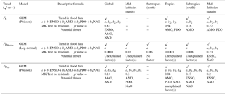
Our hypothesis (i.e., H4) is that the detected time trend is due to cyclical climate influences (i.e., oscillatory behavior) associated with the large-scale ocean–atmospheric interactions as recorded in the ENSO, AMO, PDO, and NAO indices. The corresponding residual time-trend analysis from the models explains whether the long-term natural variability dominates the trends. We considered Poisson distribution as the link function for F_C and $F_{{\mathrm{D}}_{\mathrm{90}}}$ and $F_{{\mathrm{D}}_{\mathrm{Median}}}$ in the GLM framework since they represent the counts. The detailed information on the GLM's outputs, best-choice explanatory variables, and the MK test's outputs on the residuals is shown in Table 8. The most important remarks from Table 8 are given below.

1. ENSO, AMO, and NAO are related to F_C at the global scale. There is no statistically significant trend in the residuals of the model, indicating that the trend initially observed in the global flood frequency data could be in part due to the variability in these indices. AMO and PDO in the tropics, AMO in the subtropics, and AMO and PDO in the midlatitudes (S) are the climate indicators that are dominant in explaining the variability in the flood frequency. The trend in the residuals is nonexistent. Together, we can see that the monotonic trend initially observed in the frequency of floods at the global and the sub-spatial scales may be due to the variability in the climate and atmospheric teleconnections. Ward et al. (2016) and Emerton et al. (2017) have previously demonstrated the role of ENSO in modulating global floods. In addition, Hodgkins et al. (2017) demonstrated recently that AMO has a significant negative (positive) relationship with 25- and 50-year flood occurrence for large (medium) catchments in North America (Europe). Our results corroborate with their remarks along with showing that the decadal oscillations also modulates the floods both at the global scale and in each latitudinal belt.

2. We did not find any significant climate indicators that can explain the variability in the median of the floods except for the midlatitudes (S). However, as we pointed out before, given the limited data available at this latitudinal belt, we do not further interpret these climate indicators as causing the trends. There should be one or a set of inexplicable factor(s) beyond climate teleconnections that might drive the observed trend in $F_{{\mathrm{D}}_{\mathrm{Median}}}$. We speculate that this increase relates to improved instrumentations and LULC conditions among others.

3. AMO and NAO have an association with $F_{{\mathrm{D}}_{\mathrm{90}}}$ at the global scale. There is no statistically significant trend in the residuals after adjusting for the background variance. In the midlatitudes (N), the trends in the extreme flood duration values (i.e., $F_{{\mathrm{D}}_{\mathrm{90}}}$) can be explained using AMO, PDO, and NAO. In the tropics, AMO, PDO, and NAO are related to the $F_{{\mathrm{D}}_{\mathrm{90}}}$, but we still observe a statistically significant trend after adjusting for this factor. In contrast, the trend in $F_{{\mathrm{D}}_{\mathrm{90}}}$ across the subtropics (S) can be related to ENSO, AMO, and NAO. ENSO and NAO can explain the trends across the midlatitudes (S).

• H4. In summary, we have approached the explanation of observed trends in an exploratory spirit and formulated models based on well-known atmospheric teleconnections. We see that the observed trends in flood frequency across the globe and tropics can be largely linked to the decadal and multidecadal climate variability. Regarding the flood duration, the observed trends in the median could not be associated with any of these climate factors, while extreme flood duration can be partially associated with AMO for the globe and tropics and ENSO for the southern subtropics and midlatitudes. We note that the time series (both observed variables and exogenous variables) may have autocorrelation structure that may manifest as a trend in limited data. Detection of autocorrelation before ascribing trends is important. We investigated for any structured autocorrelation in the residuals after accounting for the exogenous variables and found none. We did not examine the effect of the lagged dependence of the climate variables here. One can develop models in which an appropriate lag can be chosen based on the model performance.

Table 8 Summary of generalized linear model (GLM) results relating selected predictors to flood frequency (F_C), the median and 90th percentile of flood durations (F_D) for the global scale, and over five latitudinal belts from 1985 to 2015.

4.3 Comparison of results to recent studies

To our knowledge, this study is the first analysis of global flood events that exclusively focuses on the variability in the flood duration using the DFO dataset over the last 3 decades (i.e., 1985–2015). In this part, we are corroborating the presented results here with the most relevant previous studies. A high number of recent flood studies have focused on the regional scale, and/or have used the flood duration to calculate the flood magnitude (i.e., log × duration × severity × affected area). For instance, Halgamuge and Nirmalathas (2017) analyzed the DFO data from 1985 to 2016 and concluded that there had been a slight increase in the flood severity in both India and Australia. Similarly, it was reported by Kundzewicz et al. (2014, 2017a, b) that there is an increasing tendency in the number of floods with large magnitude and severity in Europe. These are consistent with our findings.

Several flood-related studies analyzed the trends in the annual maximum streamflow and/or precipitation across multiple spatiotemporal scales. For example, an increasing trend in annual maximum precipitation intensities was found by Min et al. (2011) in addition to the increasing trend in the extreme precipitation (Lehmann et al., 2015) at the global scale, but the catchment characteristics and river geomorphology can substantially regulate the streamflow regimes despite the intensified rainfall trends (Hall et al., 2014). Recently, Do et al. (2017) used the Global Runoff Data Center (GRDC) database to investigate the potential trends in the annual maximum streamflow and found decreasing trends for many stations in western North America but increasing trends in eastern North America, some parts of Europe and South America, and southern Africa. A complete comparative analysis is required in this regard, especially to identify the DFO locations with the river basins and then analyze the trends in those river basins. We believe that this involves developing a separate study in the future.

5 Conclusions

A global assessment of flood events is performed here, focusing on the flood frequencies and duration characteristics at different global–latitudinal–country scales from the year 1985 to 2015. The comprehensive assessment of the frequencies of flood events and characteristics of the probability distribution of flood durations presented here is the very first large-scale study of “actual” flood events worldwide focusing on understanding the temporal changes over the last 3 decades. It was verified here that the frequency of floods increased at the global scale, tropics, subtropics (S), and midlatitudes (S). Selected metrics of the flood duration showed a monotonic increasing trend for the median (at all spatial scales), MAD (across the globe, tropics, and subtropics – N), resistant skewness (across the globe, tropics, subtropics – S, and midlatitudes – S), and extremes (all spatial scales except the subtropics – N). More importantly, we find that the frequency of moderate- and long-duration floods has increased recently, but remains unchanged for the short-duration floods at all spatial scales. The trends in the flood frequency and extreme durations at a global scale can be largely ascribed to ENSO, AMO, and NAO, the interannual to decadal to multidecadal modes of variability, while the trend in the median flood durations remains unexplained. An overall summary is presented below.

• The frequency of flood events has increased; the year 2003 is recognized as the year with the maximum number of flood occurrences across all spatial scales; however much of this increase is within the long-term decadal to bi-decadal climate cycles.

• There is a statistically significant trend in the moments of the flood duration at the global scale, tropics, subtropics, and midlatitudes; the extreme floods post-2000 are more than 30 days as opposed to less than 20 days in the 1980s and 1990s. These trends in extreme flood durations ($F_{{\mathrm{D}}_{\mathrm{90}}}$) can be related to climate teleconnections, whilst the trend in the median is still unexplained.

• The yearly number of moderate- and long-duration flood occurrences increased (from before to after the 2000s) by a factor of 4 and 2.5 events per year across the tropics and midlatitudes (N), respectively.

• There was no monotonic trend observed in the frequencies of short-duration floods (i.e., flood duration of 1 to 7 days) across all the spatial scales.

• Comparison of the DFO flood events with the corresponding GRDC streamflow over the midlatitudes (N) and subtropics (N) (locations that had common records) reveals that the reported flood events by the DFO are reasonably reliable. For instance, 90 % of the events contain less than 7 days of deviation in their flood durations.

In addition, we also presented a simple overview of the vulnerability profile for different countries. This can be helpful to inform and improve the flood warning systems tailored to the various types and resource management practices during the post-disaster responses. Furthermore, with increasing globalization, countries are now interdependent through supply chain networks to achieve streamlined production and overall cost reductions. A country-level understanding of the exposure to different types of floods can help more accurately predict the vulnerable nodes that might cause a systemic network failure. It can also provide the necessary analysis for pricing and portfolio risk management for the agencies that insure and hedge against the flood losses.

While this study explores the trends in the frequency and duration of global floods, especially the long-duration floods, it is necessary to investigate the cause–effect mechanism of these trends along with socioeconomic variables to fully understand the emergence of floods. Understanding these hierarchical layers will provide us with comprehensive information and realization that can be translated into better defining the multiscale flood risk management and damage control strategies.

Appendix A: Nonparametric trend test

The nonparametric rank-based Mann–Kendall (MK) test is widely applied to detect the monotonic trend (i.e., a gradual change over time with consistency in direction) in climatic or environmental time series (Kendall, 1948; Mann, 1945). It is an appropriate approach to be employed for the type of variables that exhibit skewness around the general relationship (Helsel and Hirsch, 1992). The MK's null hypothesis (H₀) is that there is no monotonic trend (i.e., $-Z_{\mathrm{1}-\frac{\mathit{\alpha }}{\mathrm{2}}}$ ≤ Z_MK ≤ $Z_{\mathrm{1}-\frac{\mathit{\alpha }}{\mathrm{2}}}$) (Hirsch, 1992). A failure to reject H₀ indicates that the data are not sufficient to conclude that a trend might be existing, bounded to that specified level of confidence (Meals et al., 2011). The MK test is based on the S statistic as the sum of integers given in the form

$$\begin{array}{ll}{\displaystyle }S& {\displaystyle }=\sum _{p=\mathrm{1}}^{T-\mathrm{1}}\sum _{q=p+\mathrm{1}}^T\mathrm{Sign}\left(y_q-y_p\right),\mathrm{where}\mathrm{Sign}\left(y_q-y_p\right)\\ \text{(A1)}& {\displaystyle }& {\displaystyle }=\left\{\begin{array}{ll}+\mathrm{1}& \mathrm{if}\left(y_q-y_p\right)>\mathrm{0}\\ \mathrm{0}& \mathrm{if}\left(y_q-y_p\right)=\mathrm{0}\\ -\mathrm{1}& \mathrm{if}\left(y_q-y_p\right)<\mathrm{0}\end{array}\right..\end{array}$$

Also,

$$\begin{array}{}\text{(A2)}& {\displaystyle }{\displaystyle }{Z}_{\mathrm{MK}}=\left\{\begin{array}{ll}{\displaystyle \frac{S-\mathrm{1}}{\sqrt{\mathrm{Var}\left(S\right)}}}& \mathrm{if}S>\mathrm{0}\\ \mathrm{0}& \mathrm{if}S=\mathrm{0}\\ {\displaystyle \frac{S+\mathrm{1}}{\sqrt{\mathrm{Var}\left(S\right)}}}& \mathrm{if}S<\mathrm{0}\end{array}\right.,\end{array}$$

where T is the total number of observations and y_q and y_p are the data values in the time series p and q (p > q), respectively. Hence, three cases can be associated with the S value derived from Eq. (A1) (Helsel and Hirsch, 1992) as

1. it is a large positive number: an upward trend is observed since the later-measured values tend to be larger than earlier ones;

2. it is a large negative number: a downward trend is indicated since the later values tend to be smaller than earlier ones;

3. it is an absolute small number: no trend is indicated.

Further, the Kendall's tau (τ) nonparametric correlation coefficient and Sen's slope (β) (i.e., rate of consistent change) (Sen, 1968) can be computed as

$$\begin{array}{ll}{\displaystyle }& {\displaystyle }\mathit{\tau }={\displaystyle \frac{S}{\frac{T(T-\mathrm{1})}{\mathrm{2}}}};\mathrm{and}\mathit{\beta }=\mathrm{median}\left\{{\displaystyle \frac{y_q-y_p}{x_q-x_p}}\right\},\\ \text{(A3)}& {\displaystyle }& {\displaystyle }p=\mathrm{1},\mathrm{2},\mathrm{\dots },T-\mathrm{1}\mathrm{and}q=\mathrm{2},\mathrm{3},\mathrm{\dots },T\end{array}$$

where Kendall's tau (τ) value is between −1 and +1 (similar to correlation coefficient in linear regression analysis).

Appendix B: Comparing the DFO's flood database with the GRDC and EM-DAT databases

B1 Validating the DFO's flood duration using the GRDC river discharge measurements

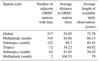
We validated the reported flood statistics in the DFO database with in situ discharge observations from the Global Runoff Database from GRDC (the Global Runoff Data Centre, 56068 Koblenz, Germany, 2013, http://grdc.bafg.de). The GRDC global-scale streamflow dataset maintains records of more than 9000 stations with an average available length of 42 years per station. From the 4311 DFO global flood events, we found 517 stations in the GRDC database that have a temporal span matching 1985–2015 and are within a radial distance of 110 km (≈ 1^∘ radial distance). Among these stations, 319 are found in the midlatitudes (N) and 122 are found in the subtropics (N). Further, these stations are predominantly located in the United States, Europe, and South Africa. A summary of the identified GRDC stations in this validation across different spatial scales is presented in Table B1.

Table B1 Summary of GRDC stations (< 110 km) with available daily observations (at least) from 1985 to 2015 adjacent to the corresponding reported DFO flood events.

We employed the following procedure to validate this common record.

1. Three flow exceedance thresholds (Q^*) as the 90th, 95th, and 99th percentile of the entire daily streamflow time series are calculated for each station separately. These thresholds for flood definition are consistent with earlier studies on this subject (e.g., Asadieh and Krakauer, 2017; Koirala et al., 2014; Wu et al., 2012, 2014).

2. The start and end dates of a flood event in a year based on the DFO database are delineated from the daily time series of the GRDC streamflow in that year.

3. Then, the total number of day(s) within the DFO's flood span when the daily streamflow exceeds the threshold (Q^*) is recorded as the GRDC's flood duration.

4. The difference between these two estimates is calculated as $F_{\mathrm{D}}^{\mathit{\left\{}\mathrm{DFO}\mathit{\right\}}}$ − $F_{\mathrm{D}}^{\mathit{\left\{}\mathrm{GRDC}\mathit{\right\}}}$.

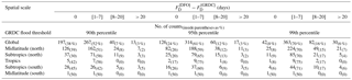
If the GRDC flood duration is as long as the flood duration of the DFO, we consider this to be a perfect match and the difference is 0. If GRDC did not exhibit a threshold exceedance flow during the DFO span, we consider this to be a miss and the difference will be as high as the flood duration for the DFO. Hence the absolute error is between 0 and $F_{\mathrm{D}}^{\mathit{\left\{}\mathrm{DFO}\mathit{\right\}}}$. We group this error into four categories: 0, [1–7], [8–20), and 21 days and above for each spatial unit. The results are presented in Table B2.

At the global scale and over the midlatitudes (N), for a threshold of the 90th percentile, up to 90 % of the events have an error of less than 7 days, indicating that the GRDC stations had experienced threshold exceedance floods when the DFO reported a flood. Even if we increase the threshold to the 95th percentile, we still have up to 85 % of the events with a deviation of less than 7 days. A similar pattern is seen for the subtropics (N). We refrain from interpreting the error results for the other spatial units as most of the GRDC matching data are only found in the midlatitudes (N) and subtropics (N).

Despite certain uncertainties in calculating flood duration (such as the distance between the GRDC station and the location of a flood event, anthropogenic inputs to the nature of flow rates, and a physical streamflow exceeding threshold that could precisely mimic the occurrence of a realistic flood event), it can be concluded that around 80 % of GRDC stations in this comparison could verify that the recorded flood information in the DFO including the start–end dates and flood duration parameters is reliable and would provide a certain path towards assessment of global flood events since 1985.

B2 Comparing the DFO's flood frequency with the EM-DAT database

We corroborated the global DFO's flood frequency with the flood frequency data available at global scale from the EM-DAT database (the Emergency Events Database, http://www.emdat.be/database) during the same time frame (1985 to 2015). As presented in Fig. B1, we can see that the original EM-DAT flood frequency time series (which is based on the reporting information) compares well with the DFO data (which are based on both satellite observations and reporting information). It should be noted that for a disaster to be recorded in the EM-DAT database, at least one of the following criteria must be satisfied: (1) 10 or more people reported killed, (2) 100 or more people reported affected, (3) there was the declaration of a state of emergency, and (4) there was a call for international assistance. We see a similar trend in EM-DAT data as in the DFO data, indicating a potential increase in floods due to various causes. It can be also inferred that the DFO is collecting more flood information, especially those events that occur in the regions with zero access to reporting facilities. The Pearson correlation coefficient between these two flood frequency datasets is 0.636 with a p value = 0.0001 (it is significant at the 5 % significance level).

B3 Distribution of start and end dates of the DFO flood events within a month

We investigated the DFO-reported flood events from 1985 to 2015 in terms of the distribution of the flood beginning date and flood end date within each month. For the starting date of flood, there are less than 5 % (194 events) out of 4311 events that have been reported with the flood beginning date as the middle of the month. There are 282 events reported on the first day of the month. Together, the first and the middle day of the month account for a total of 476 out of 4311 events (≈ 11 %). Furthermore, days 1, 5, 10, 15, 20, and 25 also have an increased number of flood counts (≈ 4 %), suggesting a reporting bias (likely rounding off of the start date to a number that can be divided by 5). An exploration of the locations of these 194 and 282 events over the 31 years revealed no specific spatial pattern (not shown here). Regarding the end date of the flood, 4.12 % (174 events) and 3.62 % (153 events) of total floods were reported to be terminated in the middle and beginning of the month, respectively. Figure B2a and b present, respectively, the distribution of flood beginning and end dates within each month at the global scale from 1985 to 2015. There is a wide distribution of the timing of the floods happening on different days of the month, which indicates that they are randomly occurring across the globe and the timing distribution also indicates a uniform spread across the month.

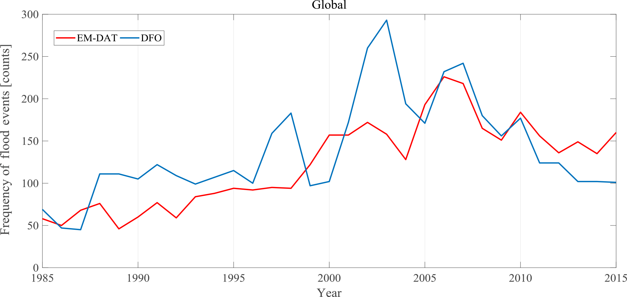
Figure B1 Frequency of flood events from the DFO database and EM-DAT at the global scale (1985–2015).

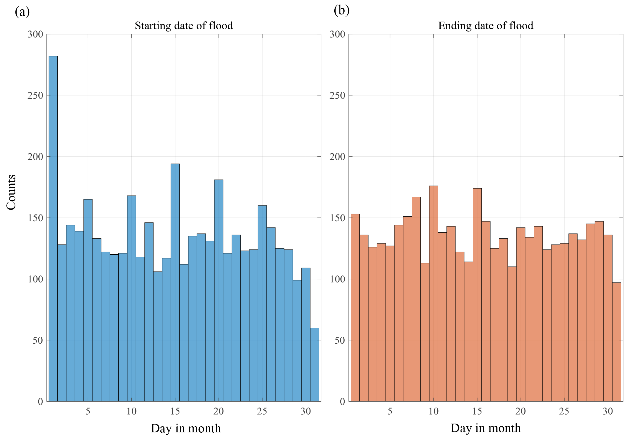
Figure B2 Distribution of the start (a) and end dates (b) of the floods within a month from the DFO database at the global scale (1985–2015).

Table B2 Comparing flood duration (F_D) reported by the DFO and calculated from the GRDC ground-based observations for the global scale and over five latitudinal belts. Three flood-related exceeding thresholds (i.e., 90th, 95th, and 99th) are derived from the entire daily observations of the GRDC stations located adjacent to the centroid of the flood event reported by the DFO.