the Creative Commons Attribution 3.0 License.
the Creative Commons Attribution 3.0 License.
Contrasting terrestrial carbon cycle responses to the 1997/98 and 2015/16 extreme El Niño events
Ning Zeng
Meirong Wang
Fei Jiang
Hengmao Wang
Ziqiang Jiang
Large interannual atmospheric CO2 variability is dominated by the response of the terrestrial biosphere to El Niño–Southern Oscillation (ENSO). However, the behavior of terrestrial ecosystems differs during different El Niños in terms of patterns and biological processes. Here, we comprehensively compare two extreme El Niños (2015/16 and 1997/98) in the context of a multi-event “composite” El Niño. We find large differences in the terrestrial carbon cycle responses, even though the two events were of similar magnitude.
More specifically, we find that the global-scale land–atmosphere carbon flux (FTA) anomaly during the 1997/98 El Niño was 1.64 Pg C yr−1, but half that quantity during the 2015/16 El Niño (at 0.73 Pg C yr−1). Moreover, FTA showed no obvious lagged response during the 2015/16 El Niño, in contrast to that during 1997/98. Separating the global flux by geographical regions, we find that the fluxes in the tropics and extratropical Northern Hemisphere were 1.70 and −0.05 Pg C yr−1 during 1997/98, respectively. During 2015/16, they were 1.12 and −0.52 Pg C yr−1, respectively. Analysis of the mechanism shows that, in the tropics, the widespread drier and warmer conditions caused a decrease in gross primary productivity (GPP; −0.73 Pg C yr−1) and an increase in terrestrial ecosystem respiration (TER; 0.62 Pg C yr−1) during the 1997/98 El Niño. In contrast, anomalously wet conditions occurred in the Sahel and East Africa during 2015/16, which caused an increase in GPP, compensating for its reduction in other tropical regions. As a result, the total 2015/16 tropical GPP and TER anomalies were −0.03 and 0.95 Pg C yr−1. GPP dominance during 1997/98 and TER dominance during 2015/16 accounted for the phase difference in their FTA. In the extratropical Northern Hemisphere, the large difference occurred because temperatures over Eurasia were warmer during the 2015/16, as compared with the cooling seen during the 1997/98 and the composite El Niño. These warmer conditions enhanced GPP and TER over Eurasia during the 2015/16 El Niño, while these fluxes were suppressed during 1997/98. The total extratropical Northern Hemisphere GPP and TER anomalies were 0.63 and 0.55 Pg C yr−1 during1997/98, and 1.90 and 1.45 Pg C yr−1 during 2015/16, respectively. Additionally, wildfires played a less important role during the 2015/16 than during the 1997/98 El Niño.
- Article
(48039 KB) - Full-text XML
- BibTeX
- EndNote


The atmospheric CO2 growth rate has significant interannual variability, greatly influenced by the El Niño–Southern Oscillation (ENSO) (Bacastow, 1976; Keeling et al., 1995). This interannual variability primarily stems from terrestrial ecosystems (Bousquet et al., 2000; Zeng et al., 2005). There is also a general consensus that the tropical terrestrial ecosystems account for the terrestrial carbon variability (Zeng et al., 2005; Cox et al., 2013; Peylin et al., 2013; Wang et al., 2013, 2016). They tend to release anomalous levels of carbon flux during El Niño episodes, and take up carbon during La Niña events (Zeng et al., 2005; Wang et al., 2016). Recently, Ahlstrom et al. (2015) further suggested that ecosystems in semi-arid regions dominated the terrestrial carbon interannual variability, with a 39 % contribution.
The terrestrial dominance primarily results from the driver–response mechanisms in climate variability (especially in temperature and precipitation) caused by ENSO and plant/soil physiology (Tian et al., 1998; Zeng et al., 2005; Wang et al., 2016; Jung et al., 2017). The land–atmosphere carbon flux (FTA – positive sign meaning a flux into the atmosphere) can mainly be attributed to the imbalance between the gross primary productivity (GPP) and terrestrial ecosystem respiration (TER) according to , where the carbon flux from wildfires (Cfire) is generally much smaller than the GPP or TER. Variations in each, or all, result in the changes in FTA.
Based on a dynamical global vegetation model (DGVM), Zeng et al. (2005) found that net primary productivity (NPP) contributed to almost three quarters of the tropical FTA interannual variability. Multi-model simulations involved in the TRENDY project and CMIP5 have consistently suggested that NPP or GPP dominate the terrestrial carbon variability (Piao et al., 2013; Ahlstrom et al., 2015; Kim et al., 2016; Wang et al., 2016).
These biological process analyses suggest that precipitation variation is the dominant climate factor in controlling FTA interannual variability (Tian et al., 1998; Zeng et al., 2005; Qian et al., 2008; Ahlstrom et al., 2015; Wang et al., 2016). Qian et al. (2008) calculated the contributions of tropical precipitation and temperature as 56 and 44 %, respectively, based on model sensitivity experiments. Eddy covariance network observations have suggested that the interannual carbon flux variability over tropical and temperate regions is controlled by precipitation, while boreal ecosystem carbon fluxes are more affected by temperature and radiation (Jung et al., 2011). At the same time, there is a significant positive correlation between the atmospheric CO2 growth rate and mean tropical land temperature (Cox et al., 2013; Wang et al., 2013, 2014; Anderegg et al., 2015). Regression analysis indicates an anomaly of approximately 3.5 Pg C yr−1 in the CO2 growth rate with a 1 ∘C increase in tropical land temperature, whereas a weaker interannual coupling exists between the CO2 growth rate and tropical land precipitation (Wang et al., 2013). Clark et al. (2003) and Doughty et al. (2008) also concluded, based on in situ observations, that warming anomalies can reduce tropical tree growth and CO2 uptake. Therefore, considering this strong emergent linear relationship, these studies (Clark et al., 2003; Doughty et al., 2008; Cox et al., 2013; Wang et al., 2013, 2014; Anderegg et al., 2015) have suggested that temperature dominates the interannual variability of the FTA or CO2 growth rate. To reconcile these contradictory reports, Jung et al. (2017) showed that the temporal and spatial compensatory effects in water availability link the yearly global FTA variability to temperature. Fang et al. (2017) suggested an ENSO-phase-dependent interplay between water availability and temperature in controlling the tropical terrestrial carbon cycle response to climate variability.
Apart from these long-term time series studies on the interannual FTA or CO2 growth rate variability, we should keep in mind that the terrestrial carbon cycle responds in a unique way in terms of its strength, spatial patterns, and biological processes to every El Niño/La Niña event, because of the ENSO diversity with different spatial patterns and evolutions (Schwalm, 2011; Capotondi et al., 2015). For example, wildfires played an important role in the FTA anomalies during the 1997/98 El Niño (van der Werf et al., 2004). Therefore, it is important to have clear insight into the impacts of individual ENSO events on the terrestrial carbon cycle, and this is best achieved through representative case studies. Recently, one of the three extreme El Niño events in recorded history occurred in 2015/16 (https://www.esrl.noaa.gov/psd/enso/current.html). Because of the interference of the El Chichón eruption during the extreme El Niño case in 1982/83, we chose to compare in detail the response of terrestrial ecosystems in the other two extreme El Niño events, i.e., in 1997/98 and 2015/16, in the context of a multi-event “composite” El Niño, based on the VEGAS DGVM in its near-real-time framework and inversion datasets (Copernicus Atmosphere Monitoring Service (CAMS), Monitoring Atmospheric Composition & Climate (MACC), and CarbonTracker). The purpose is to clarify the different responses of biological processes in these two extreme events.
The paper is organized as follows. Section 2 describes the mechanistic carbon cycle model used, its drivers, and reference datasets. Section 3 presents the results of the total terrestrial carbon flux anomalies and spatial patterns, along with their mechanisms. Finally, a discussion and concluding remarks are provided in Sect. 4.
2.1 Mechanistic carbon cycle model and its drivers
We used the state-of-the-art VEGAS DGVM, version 2.4, in its near-real-time framework, to investigate the responses of terrestrial ecosystems to El Niño events. VEGAS has been widely used to study the terrestrial carbon cycle on its seasonal cycle, interannual variability, and long-term trends (Zeng et al., 2004, 2005, 2014). The model has also extensively participated in international carbon modeling projects, such as the Coupled Climate–Carbon Cycle Model Intercomparison Project (C4MIP; Friedlingstein et al., 2006), the TRENDY project (Sitch et al., 2015) and the Multi-scale Synthesis and Terrestrial Model Intercomparison Project (MsTMIP; Huntzinger et al., 2013). A detailed description of the model structure and biological processes can be found in the appendix of Zeng et al. (2005). We ran VEGAS at the horizontal resolution from 1901 until the end of 2016, and focused on the period from 1980 to 2016.
The climate fields and boundary forcings used to run VEGAS were as follows:
- (1)
Precipitation datasets generated by combining the Climatic Research Unit (CRU) Time-series (TS) version 3.22 (University of East Anglia Climatic Research Unit et al., 2014), NOAA's Precipitation Reconstruction over Land (PREC/L) (Chen et al., 2002), and the NOAA–NCEP Climate Anomaly Monitoring System-Outgoing Longwave Radiation Precipitation Index (CAMS-OPI) (Janowiak and Xie, 1999).
- (2)
Temperature data from the CRU TS3.22 before the year 2013, generated by combining the CRU 1981–2010 climatology and the Goddard Institute for Space Studies (GISS) Surface Temperature Analysis (GISTEMP) (Hansen et al., 2010) after 2013.
- (3)
Downward shortwave radiation from the driver datasets in MsTMIP (Wei et al., 2014) before 2010, with the value of the year 2010 repeated for subsequent years.
- (4)
The gridded cropland and pasture land use datasets integrated from the History Database of the Global Environment (HYDE) (Klein Goldewijk et al., 2011) with a linear extrapolation in 2016.
2.2 Reference datasets
We selected a series of reference datasets to compare to the VEGAS simulation. The atmospheric CO2 concentrations were from the monthly in situ CO2 datasets at the Mauna Loa Observatory, Hawaii (Keeling et al., 1976). The Niño 3.4 (120∘ W–170∘ W, 5∘ S–5∘ N) sea surface temperature anomaly (SSTA) data were from the NOAA's Extended Reconstructed Sea Surface Temperature (ERSST) dataset, version 4 (Huang et al., 2015), with a 3-month running average. We compared the CAMS (1980–2015) and MACC (1980–2014) inversion results (Chevallier, 2013) and the CarbonTracker2016 (2000–2015) with the CarbonTracker near-real-time results from 2016 (Peters et al., 2007) with VEGAS. The FTA in CarbonTracker was calculated by the sum of the posterior biospheric flux and its imposed fire emissions. The Satellite-based fire emissions were from the Global Fire Emissions Database version 4 (GFEDv4) from 1997 through 2014 (Randerson et al., 2015). Owing to the high correlation between the solar-induced chlorophyll fluorescence (SIF) and terrestrial GPP (Guanter et al., 2014), we selected the monthly satellite SIF from the GOME2_F version 26 from 2007 to 2016 (Joiner et al., 2012). We also compared the enhanced vegetation index (EVI) from MODIS MOD13C2 (Didan, 2015) with the simulated leaf area index (LAI) anomalies.
2.3 Methods
To calculate the anomalies during the El Niño events, we first removed the long-term climatology in each dataset for getting rid of seasonal cycle signals. We then detrended them based on the linear regression, because the trend was mainly caused by long-term CO2 fertilization and climate change. We used these detrended monthly anomalies to investigate the impacts of El Niño events on the terrestrial carbon cycle.
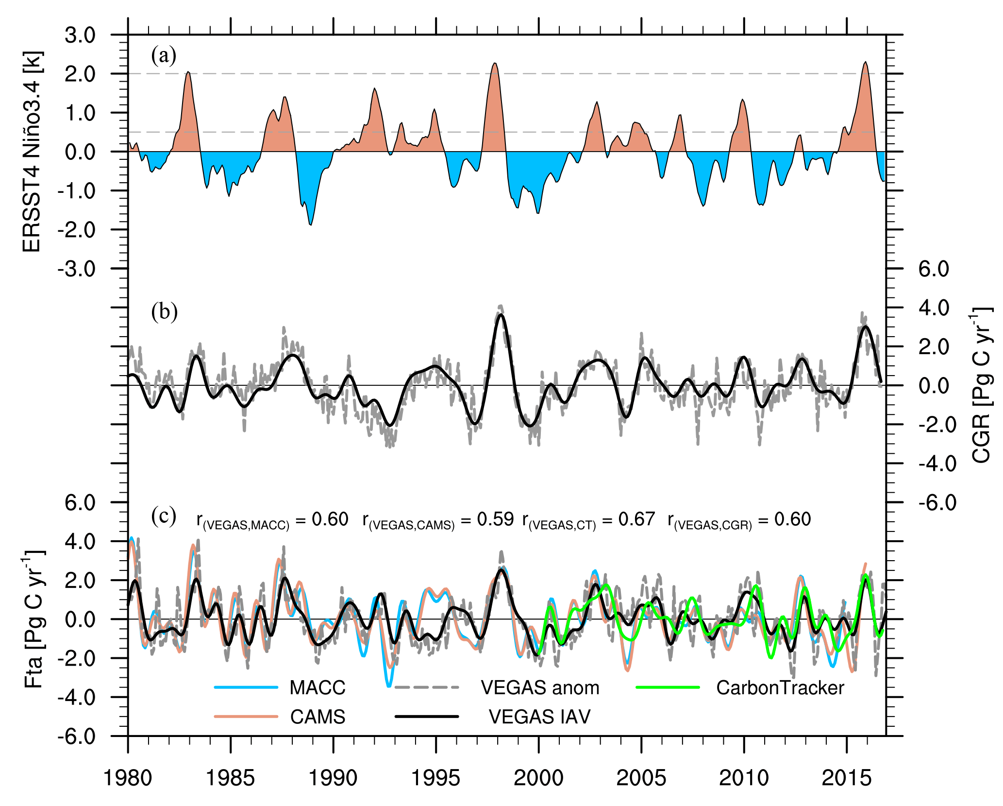
Figure 1Interannual variability (IAV) in the sea surface temperature anomaly (SSTA) and carbon cycle. (a) ERSST4 Niño3.4 Index (units: K) using the 3-month running averaged SSTA for the Niño 3.4 region (5∘ N–5∘ S, 120–170∘ W). (b) IAV in the Mauna Loa CO2 growth rate (CGR; units: Pg C yr−1). The CGR is calculated as the difference between the monthly mean in adjacent years. The dashed line is the detrended monthly anomaly and the solid line is smoothed by the Butterworth filtering. (c) IAV in the land–atmosphere carbon fluxes (FTA; units: Pg C yr−1). The blue and orange solid lines are the smoothed results of the MACC and CAMS inversions, respectively. The gray dashed line is the detrended anomaly and the black one is the smoothed result from the VEGAS model simulation. The green solid line is the smoothed CarbonTracker result.
3.1 Total terrestrial carbon flux anomalies
Three extreme El Niño events (1982/83, 1997/98, and 2015/16) occurred from 1980 to 2016, with their maximum SSTAs above 2.0 K (Fig. 1a). An El Niño event tends to anomalously increase the atmospheric CO2 growth rate (Fig. 1b); therefore, there are two significant anomalous increases in CO2 growth rate that correspond to the 1997/98 and 2015/16 El Niño events, although the maximum increase in 2015/16 was slightly less than that in 1997/98. Because of the diffuse light disturbance (Mercado et al., 2009) of the Mount El Chichón eruption during the 1982/83 El Niño on the canonical coupling between the anomalies of the CO2 growth rate anomalies and El Niño events, we mainly focused on the 1997/98 and 2015/16 El Niño events in this study. The interannual variability of the atmospheric CO2 growth rate principally originates from the terrestrial ecosystems (Fig. 1c). The correlation coefficient between the CO2 growth rate anomalies and the global FTA simulated by VEGAS was 0.60 (p<0.05). In order to evaluate the performance of the VEGAS simulation on the interannual timescale, we also present CAMS, MACC, and CarbonTracker inversion results. The CAMS and MACC inversions were nearly the same, with a correlation coefficient of approximately 0.60 (p<0.05) with VEGAS. From 2000 to 2016, CarbonTracker was highly correlated with VEGAS (r=0.67, p<0.05). These high correlation coefficients between VEGAS and the reference datasets indicate that VEGAS can capture the terrestrial carbon cycle interannual variability well.
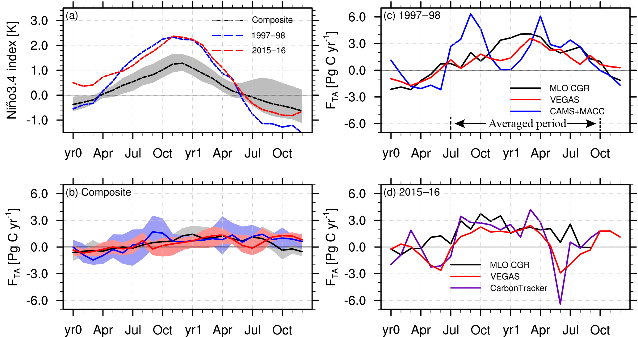
Figure 2Evolutions of the global FTA along with the development of El Niño. (a) the SSTA in the composite (black), 1997/98 (blue), and 2015/16 (red) El Niño events. (b) The FTA anomalies in the El Niño composite analysis. The black solid line denotes the Mauna Loa CGR, and the red and blue lines show the VEGAS and mean of the CAMS and MACC inversions, respectively. The shaded areas in (a) and (b) show the 95 % confidence intervals of the variables in the composite, derived in 1000 bootstrap estimates. (c) The FTA anomalies during the 1997/98 El Niño events. The arrows demonstrate the time periods during which we calculate the carbon flux anomalies listed/presented in the table and figures. (d) The FTA anomalies during the 2015/16 El Niño. The purple line denotes the result of the CarbonTracker2016 and CarbonTracker near-real-time datasets.
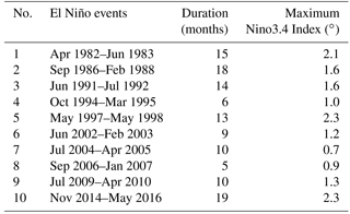
There were 10 El Niño events from 1980 to 2016, each with a different duration and strength (Table 1). According to the definition of El Niño, these 10 events can be categorized into two weak (with a 0.5 to 0.9 SSTA), three moderate (1.0 to 1.4), two strong (1.5 to 1.9), and three very strong (≥2.0) events. During the 1997/98 El Niño, the positive SSTA lasted from April 1997 to June 1998, while the positive SSTA occurred in winter 2014, and extended to June 2016 in the 2015/16 El Niño (Fig. 2a). However, every El Niño event always peaks in winter (November or December; Fig. 2a). Considering this phase-lock phenomenon in the El Niño events, we produced a composite analysis (excluding 1982/83 and 1991/92, because of the diffuse radiation disturbances) as the background responses of the terrestrial carbon cycle to El Niño events.
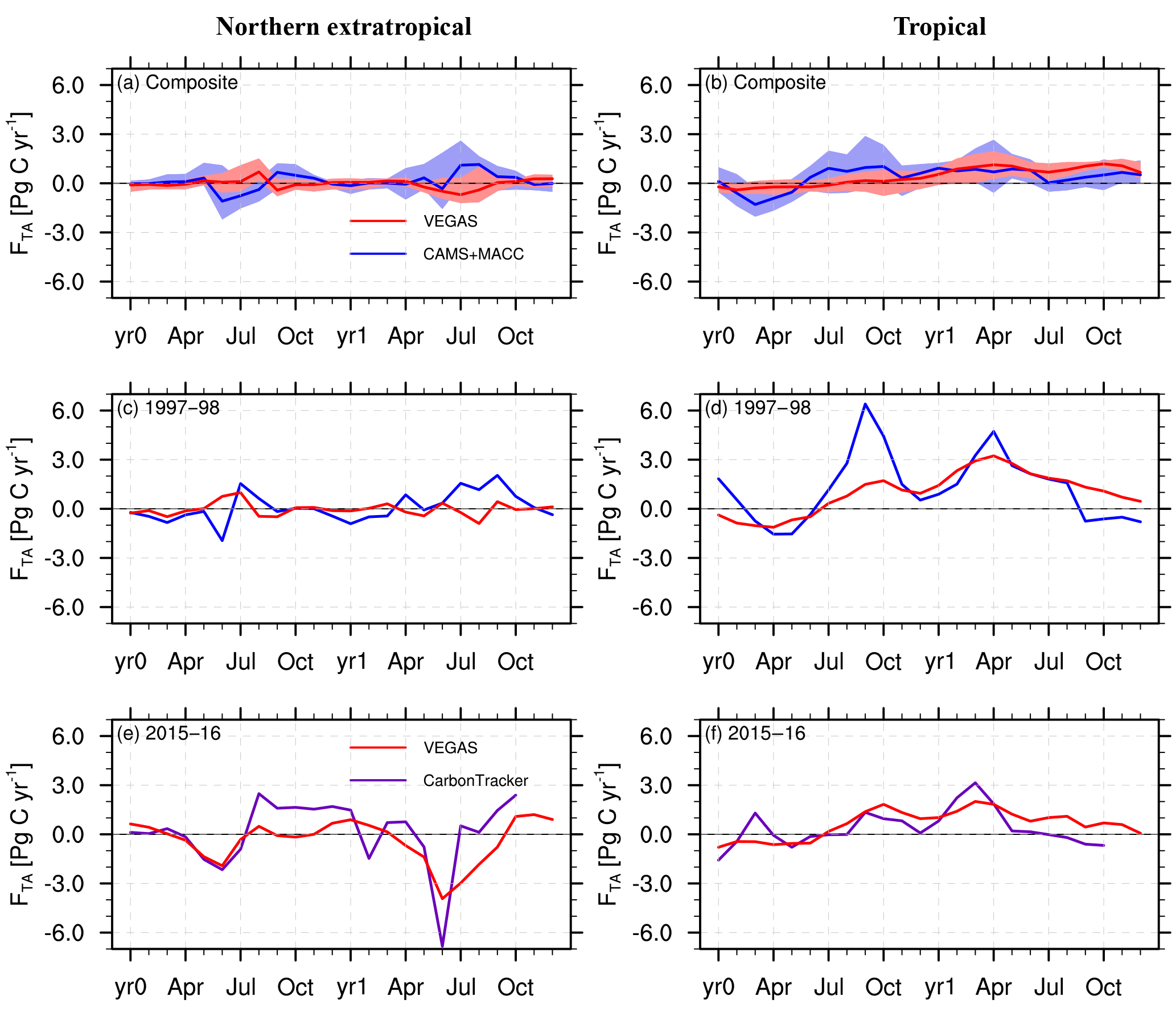
Figure 3Evolutions of FTA over the extratropical Northern Hemisphere (23∘ N–90∘ N) and tropical regions (23∘ S–23∘ N) along with the development of El Niño. (a, b) Composite results with the VEGAS simulation (red solid line) and the mean of the CAMS and MACC inversions (blue solid line). The shaded areas show the 95 % confidence intervals of the variables in the composite, derived in 1000 bootstrap estimates. (c, d) The FTA anomalies during the 1997/98 El Niño. (e, f) The FTA anomalies in the 2015/16 El Niño with VEGAS (red solid line) and CarbonTracker (purple solid line).
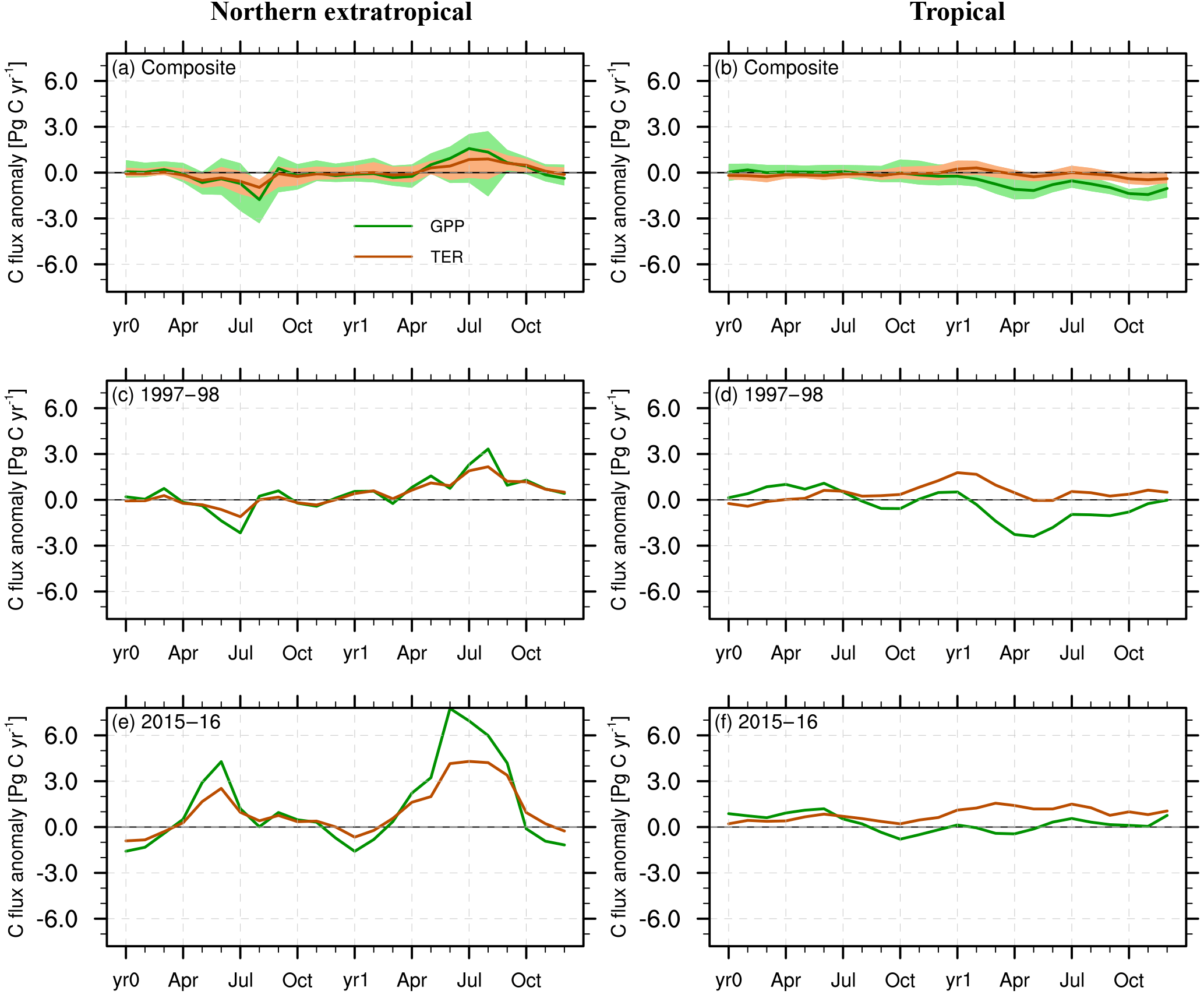
Figure 4Evolutions of gross primary productivity (GPP, green lines) and terrestrial ecosystem respiration (TER, brown lines) over the extratropical Northern Hemisphere (23∘ N–90∘ N) and tropical regions (23∘ S–23∘ N) along with the development of El Niño. (a, b) El Niño composite results. The shaded areas show the 95 % confidence intervals of the variables in the composite, derived in 1000 bootstrap estimates. (c, d) Results of the 1997/98 El Niño. (e, f) Results of the 2015/16 El Niño.
The evolution of the global FTA anomalies in VEGAS, the mean of CAMS and MACC, and CarbonTraker in the composite, 1997/98, and 2015/16 El Niño events are closely consistent with the Mauna Loa CGR anomalies (Fig. 2b–d). The peaks of the FTA and the Mauna Loa CGR anomalies in the 1997/98 and 2015/16 El Niño events were much stronger than those in the composite analysis. Importantly, there were significant terrestrial lagged responses in the composite and 1997/98 El Niño events, with the peak of the FTA anomaly occurring from March to April in the El Niño decaying year (Fig. 2b and c), consistent with previous studies (Qian et al., 2008; Wang et al., 2016). However, this lagged terrestrial response disappeared in the Mauna Loa CGR, VEGAS, and CarbonTracker in the 2015/16 El Niño (Fig. 2d). In June 2016, the FTA anomaly of VEGAS and CarbonTracker reduced significantly (the sign changed), whereas the Mauna Loa CGR reduced only slightly (no sign change; Fig. 2d). A similar phenomenon also occurred earlier, from April to July 2015. In addition, the anomalous carbon release caused by the El Niño lasted from approximately July in the El Niño developing year to October in the El Niño decaying year (Fig. 2b–d). For simplicity, we calculated the total anomalies of all El Niño events during this period in the next context, taking the terrestrial lagged responses into account (Wang et al., 2016).
Based on the major geographical regions, we separated global FTA anomaly into the extratropical Northern Hemisphere (23∘ N–90∘ N), tropical regions (23∘ S–23∘ N), and extratropical Southern Hemisphere (60∘ S–23∘ S). Because the FTA anomaly over the extratropical Southern Hemisphere is generally smaller, we mainly present the evolutions of the FTA over the extratropical Northern Hemisphere and the tropical regions in Fig. 3. Comparing the global and tropical FTA anomalies, we find that the FTA anomalies in the tropical regions dominated the global FTA during these El Niño events (Fig. 3b, d and f), in accordance with previous conclusions (Zeng et al., 2005; Peylin et al., 2013). The FTA anomalies over the extratropical Northern Hemisphere were nearly neutral in VEGAS for the composite and the 1997/98 El Niño events (Fig. 3a and c). However, there was clear anomalous uptake from April to September in 2016 simulated by VEGAS (Fig. 3e), compensating for the carbon release over the tropics (Fig. 3f). This anomalous uptake caused the globally negative FTA anomalies that occurred from May to September in 2016 (Fig. 2d). Similar anomalous uptake also occurred over the extratropical Northern Hemisphere from April to July 2015. This anomalous uptake in VEGAS was to some extent consistent with the results from CarbonTracker, and accounted for the global FTA reduction mentioned above during these periods. Comparing the behaviors between the Mauna Loa CGR and the FTA anomalies, the Mauna Loa CGR, which originates from a tropical observatory, does not reflect the signals over the extratropical Northern Hemisphere in time (Figs. 2d and 3e).
Because FTA mainly stems from the difference between TER and GPP, we present the TER and GPP anomalies in Fig. 4 to clearly explain the FTA anomalies. Anomalously negative GPP dominated the FTA anomaly in the tropics in the composite and the 1997/98 El Niño episodes, with the significant lagged responses (peak at approximately May of the El Niño decaying year; Fig. 4b and d). Furthermore, clear positive TER anomalies occurred from October 1997 to April 1998 (Fig. 4d), contributing to the tropical carbon release during this period (Fig. 3d). In contrast, anomalously positive TER dominated the FTA anomaly in the tropics during the 2015/16 El Niño, without clear lags (Fig. 4f), accounting for the disappearance of the terrestrial FTA lagged response (Fig. 2d). In the extratropical Northern Hemisphere, the increased GPP and TER from April to October were nearly identical in the composite and in 1998 (Fig. 4a and c), causing neutral FTA anomalies (Fig. 3a and c). However, the increased GPP was stronger than the increased TER from April to July 2015 and from April to September 2016 (Fig. 4e), resulting in the anomalous uptake in FTA (Figs. 2d and 3e).
Table 2Carbon flux anomalies during El Niño events, calculated as the mean from July in the El Niño developing year to October in the El Niño decaying year. Flux units are in Pg C yr−1.
a The mean value of the CAMS and MACC inversion results with
the uncertainty of their SD.
b Composite analyses exclude the 1982/83, 1991/92, and 2015/16 El
Niño events, because the former two cases were disturbed by the El
Chichón and Pinatubo eruptions, and the latter is not covered by the
inversion datasets.
We calculated the total carbon flux anomalies from July in the El Niño developing year to October in the El Niño decaying year. The composite global FTA anomaly during the El Niño events in VEGAS was approximately 0.60 Pg C yr−1, dominated by tropical ecosystems with 0.61 Pg C yr−1 (Table 2). These anomalies were comparable to the mean of the CAMS and MACC inversion results, at 0.92±0.01 globally and 0.66±0.03 Pg C yr−1 in the tropics. In these two extreme cases, a strong anomalous carbon release occurred during the 1997/98 El Niño, with a value of 1.64 Pg C yr−1, which was less than the 2.57 Pg C yr−1 in the CAMS and MACC inversions, while only 0.73 Pg C yr−1 was released during the 2015/16 El Niño, which was comparable to the 0.82 Pg C yr−1 in CarbonTracker. However, the FTA anomalies in the tropical regions dominated the global FTA anomalies in both cases, with values of 1.70 and 1.12 Pg C yr−1 in VEGAS, respectively. Furthermore, anomalous carbon uptake simulated by VEGAS over the extratropical Northern Hemisphere canceled out the 0.52 Pg C yr−1 anomalous release in the tropics during the 2015/16 El Niño, whereas it was neutral (−0.05 Pg C yr−1) in the 1997/98 El Niño. The FTA anomaly was relatively smaller in the extratropical Southern Hemisphere.
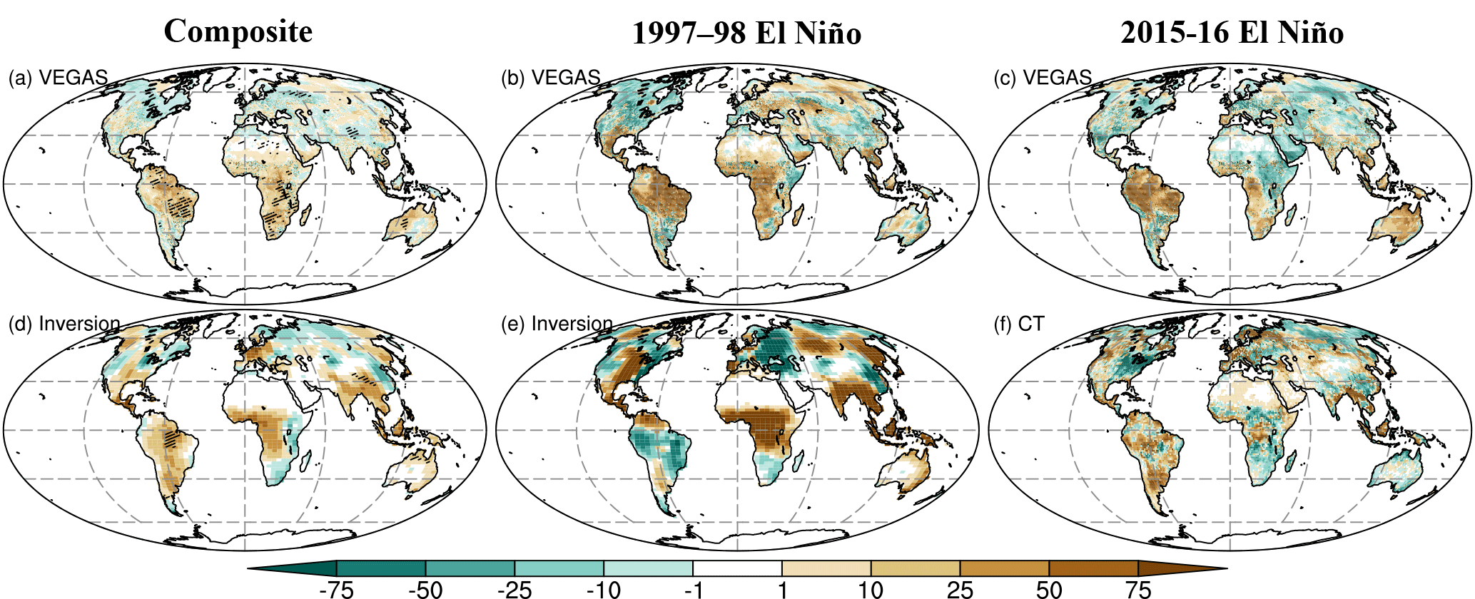
Figure 5Spatial FTA anomalies calculated from July in the El Niño developing year to October in the El Niño decaying year (units: ). (a–c) Results of the composite, 1997/98, and 2015/16 El Niño events simulated by VEGAS, respectively. (d–e) The averaged results of CAMS and MACC in the composite and 1997/98 El Niños. (f) The 2015/16 El Niño FTA anomaly in CarbonTracker. The stippled areas in (a) and (d) are significant above the 90 % level, estimated by Student's t test.
In terms of the biological processes, the GPP (−0.73 Pg C yr−1) and TER (0.62 Pg C yr−1) in the tropics together drove the anomalous FTA during 1997/98, while the TER (0.95 Pg C yr−1) mainly drove the anomalous FTA during 2015/16, with a near-neutral GPP of −0.03 Pg C yr−1 (Table 2). These data confirmed that the GPP played a more important role in the 1997/98 event, while TER was dominant during the 2015/16 El Niño. In the extratropical Northern Hemisphere, GPP and TER canceled each other out. They were 0.13 and 0.08 Pg C yr−1 in the composite analysis, and 0.63 and 0.55 Pg C yr−1 in the 1997/98 El Niño, respectively, causing the near-neutral FTA anomaly in that region. However, the GPP and TER in the 2015/16 El Niño were much stronger than those in the composite or the 1997/98 El Niño. Importantly, the GPP (1.90 Pg C yr−1) was stronger than the TER (1.45 Pg C yr−1) in the 2015/16 El Niño, causing the significant carbon uptake. The FTA anomaly caused by wildfires also played an important role during the 1997/98 El Niño, with a global value of 0.42 Pg C yr−1 in VEGAS, which was consistent with the GFED fire data product (0.82 Pg C yr−1). The effect of wildfires on the FTA anomaly during the 1997/98 El Niño episode has been previously suggested by van der Werf et al. (2004), whereas it was close to zero (0.05 Pg C yr−1) during the 2015/16 El Niño.
Figure 6Anomalies of soil wetness, air temperature (units: K), GPP (), and TER () from July in the El Niño developing year to October in the El Niño decaying year in the composite, 1997/98, and 2015/16 El Niño episodes, respectively. (a–d) Results of the composite analyses. The stippled areas are significant above the 90 % levels estimated by Student's t test. (e–h) Anomalies during the 1997/98 El Niño. (i–l) Anomalies during the 2015/16 El Niño.
3.2 Spatial features and its mechanisms
The regional responses of terrestrial ecosystems to El Niño events are inhomogeneous, principally due to the anomalies in climate variability. In the composite El Niño analysis (Fig. 5a), land consistently released carbon flux in the tropics, while there was an anomalous carbon uptake over North America as well as central and eastern Europe. These regional responses were generally consistent with the CAMS and MACC inversion results (Fig. 5d).
During the 1997/98 El Niño episode, the tropical responses were analogous to the composite results, except for stronger carbon releases. North America and central and eastern China had stronger carbon uptake, whereas Europe and Russia had stronger carbon release (Fig. 5b). However, during the 2015/16 El Niño, anomalous carbon uptake occurred over the Sahel and East Africa, compensating for the carbon release over the other tropical regions (Fig. 5c). This made the total FTA anomaly in the tropics in 2015/16 less than that in 1997/98 (Fig. 3d and f; and Table 2). North America had anomalous carbon uptake, similar to that in the composite and the 1997/98 El Niño, while central and eastern Russia had anomalous carbon uptake during the 2015/16 El Niño (Fig. 5c), which was opposite to the carbon release in the composite and the 1997/98 El Niño. This opposite behavior of the boreal forests over central and eastern Russia clearly contributed to the total uptake over the extratropical Northern Hemisphere (Table 2). Moreover, these regional responses during the 2015/16 El Niño were significantly consistent with the CarbonTracker result (Fig. 5f).
To better explain these regional carbon flux anomalies, we present the main climate variabilities of soil wetness (mainly caused by precipitation) and air temperature, and the biological processes of GPP and TER in Fig. 6. In the composite analyses, the soil wetness is generally reduced in the tropics (Fig. 6a), causing the widespread decrease in GPP (Fig. 6b), which has been verified by model sensitivity experiments (Qian et al., 2008). At the same time, air temperature was anomalously warmer, contributing to the increase in TER. However, the drier conditions in the semi-arid regions, such as the Sahel, South Africa, and Australia, restricted this increase in TER induced by warmer temperatures (Fig. 6d). Higher air temperatures over North America largely enhanced the GPP and TER, while cooler conditions over the Eurasia reduced them (Fig. 6b–d). Wetter conditions over parts of North America and Eurasia also increased the GPP and TER to some extent (Fig. 6a).
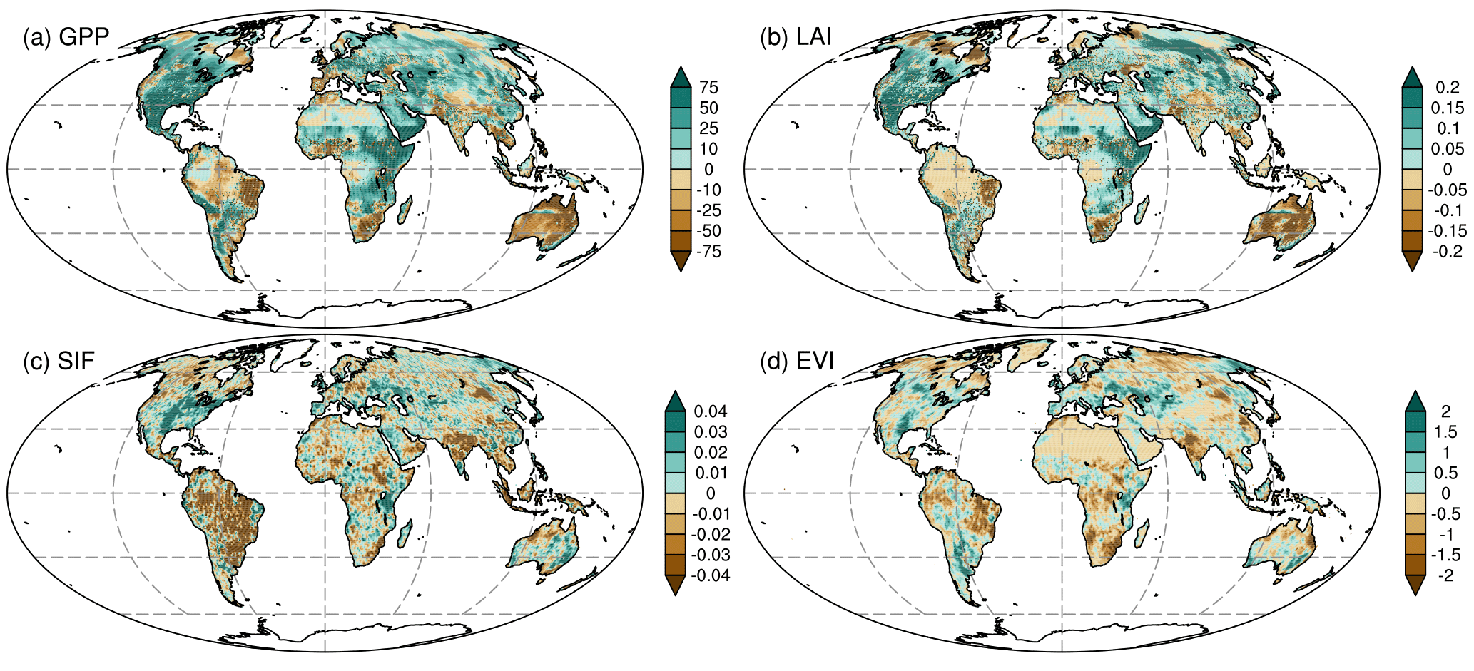
Figure 7Spatial anomalies in (a) the simulated GPP by VEGAS (units: ), (b) the simulated leaf area index (LAI; units: m2 m−2), (c) solar-induced chlorophyll fluorescence (SIF; units: ), and (d) MODIS enhanced vegetation index (EVI, ) from July 2015 to October 2016.
Comparing the composite results (Fig. 6a–d) and the 1997/98 El Niño (Fig. 6e–h), the regional patterns were almost identical, except for the difference in magnitude. In contrast, there were some differences in the 2015/16 El Niño. Over the Sahel and East Africa, the soil wetness increased due to the higher precipitation (Fig. 6i), dynamically cooling the air temperature (Fig. 6k). These wetter conditions largely benefit GPP (Fig. 6j), compensating for the reduced GPP over the other tropical regions. This caused GPP to be near neutral in the tropics, as compared to the composite and the 1997/98 El Niño (Table 2). Higher soil moisture also contributed to increased TER over the Sahel (Fig. 6l), contrary to that in the 1997/98 El Niño (Fig. 6h). This spatial compensation in GPP, together with the widespread increase in TER, accounted for the TER dominance in the tropics during the 2015/16 El Niño. Furthermore, the higher GPP resulted in the anomalous carbon uptake in that region (Fig. 5c), which partly compensated for the anomalous carbon release over the other tropical regions. This in part caused the smaller tropical FTA during the 2015/16 El Niño compared with that during 1997/98. Another clear difference occurred over the Eurasia, with almost opposite signals during the 1997/98 and 2015/16 El Niño events. During the 2015/16 El Niño over the Eurasia, air temperature was anomalously higher compared with the cooling in the composite and during the 1997/98 El Niño (Fig. 6c, g, and k). This warmth enhanced the GPP and TER (Fig. 6j and l), as compared with the reduced levels in the composite and during the 1997/98 El Niño (Fig. 6b, d, f, and h). This phenomenon explains the stronger GPP and TER anomalies, and the anomalous carbon uptake over the whole of the extratropical Northern Hemisphere (Table 2).
Recently, more attention has been paid to SIF as an effective indicator of GPP (Guanter et al., 2014). Therefore, we compared the simulated GPP and SIF variabilities on the interannual timescale. Although noisy signals in SIF occurred, it was anomalously positive over the USA, parts of Europe, and East Africa, and negative over the Amazon and South Asia, during the 2015/16 El Niño, corresponding to increased and decreased GPP, respectively (Fig. 7a and c). The match over other regions was not significant. In addition, MODIS EVI increased anomalously over North America, southern South America, parts of Europe, the Sahel, and East Africa but reduced over the Amazon, northern Canada, central Africa, South Asia, and northern Australia (Fig. 7d). These EVI anomalies corresponded well with the simulated LAI anomalies (Fig. 7b). The good match between the simulated GPP (LAI) and SIF (EVI) gives us more confidence in the VEGAS simulations.
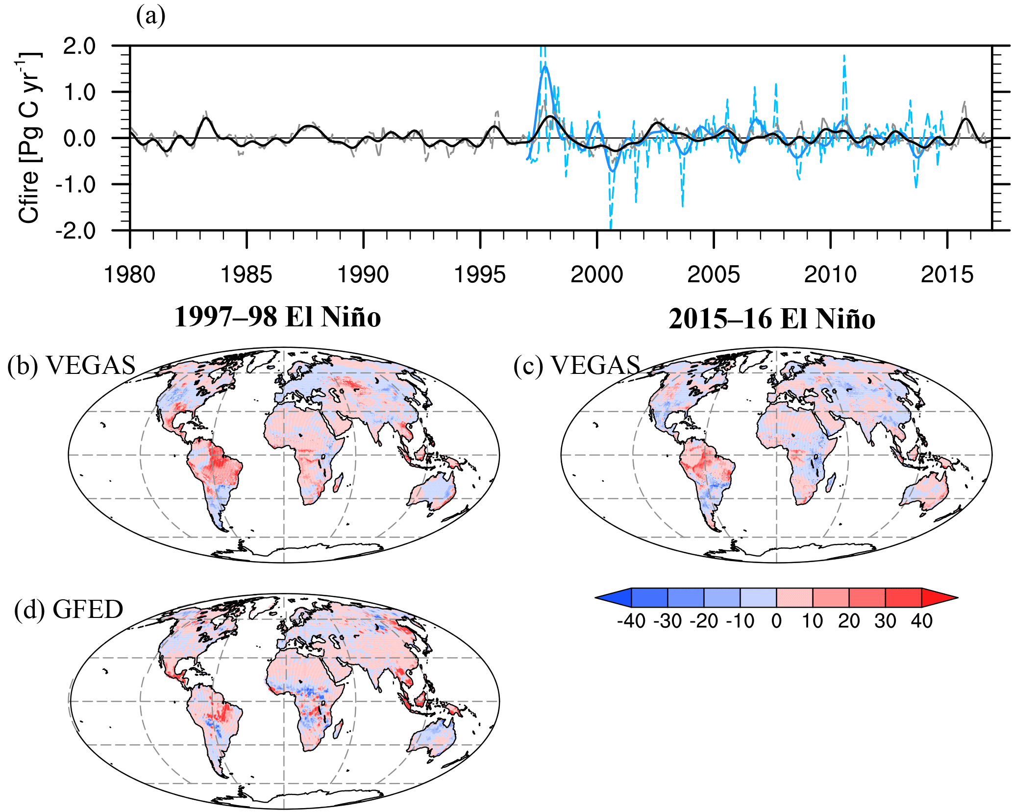
Figure 8FTA anomalies induced by wildfires. (a) Total global anomalies (Pg C yr−1). The dashed gray and solid black lines represent the anomalies simulated by VEGAS, detrended and smoothed by Butterworth filtering, respectively. The dashed and solid blue lines represent the GFED results. (b) Spatial FTA anomaly () during the 1997/98 El Niño in VEGAS. (c) Spatial FTA anomaly during the 2015/16 El Niño in VEGAS. (d) GFED anomaly during the 1997/98 El Niño episode.
Finally, wildfires, as important disturbances for FTA, always release carbon flux. Although the FTA anomalies caused by wildfires were generally smaller than the GPP or TER anomalies, they played an important role during the 1997/98 El Niño (globally, 0.42 Pg C yr−1 in VEGAS and 0.82 Pg C yr−1 in GFED; Table 2), which is consistent with previous work (van der Werf et al., 2004). The FTA anomalies caused by wildfires are shown in Fig. 8. The correlation coefficients between the simulated global FTA anomalies caused by wildfires and the GFED fire data product was 0.46 (unsmoothed) and 0.63 (smoothed; Fig. 8a), confirming that VEGAS has certain capability in simulating this disturbance. During the 1997/98 El Niño, satellite-based GFED data show that the FTA anomalies caused by wildfires mainly occurred over the tropical regions, such as the Amazon, central Africa, South Asia, and Indonesia (Fig. 8d). VEGAS also simulated the positive FTA over these tropical regions (Fig. 8b). The total tropical FTA anomalies caused by fires were 0.37 Pg C yr−1 in VEGAS and 0.72 Pg C yr−1 in GFED (Table 2). During the 2015/16 El Niño, wildfires also resulted in positive FTA anomalies over the Amazon, South Asia, and Indonesia; however, their magnitudes were smaller than those during the 1997/98 El Niño, because it was much drier during the 1997/98 event than the 2015/16 one (Fig. 6e and i). In addition, the wetter conditions over East Africa during the 2015/16 El Niño suppressed the occurrences of wildfires with the negative FTA anomalies (Fig. 8c). The total tropical FTA anomaly was 0.11 Pg C yr−1 in VEGAS (Table 2). Therefore, wildfires played a less important role during the 2015/16 event than during the 1997–98 one. The FTA anomalies caused by wildfires over the extratropics were much weaker than those over the tropics, and the match between VEGAS and GFED was poorer (Table 2; Fig. 8b and d).
The magnitudes and patterns of climate anomalies caused by different El Niño events differ. Therefore, the responses of terrestrial carbon cycle to different El Niño episodes remain uncertain (Schwalm, 2011). In this study, we compared in detail the impacts of two extreme El Niño events in recorded history (namely, the recent 2015/16, and earlier 1997/98 events) on the terrestrial carbon cycle in the context of a multi-event “composite” El Niño. We used VEGAS in its near-real-time framework, along with inversion datasets. The main conclusions can be summarized as follows:
- (1)
The simulations indicated that the global-scale FTA anomaly during the 2015/16 El Niño was 0.73 Pg C yr−1, which was nearly 2 times smaller than that during the 1997/98 El Niño (1.64 Pg C yr−1), and was confirmed by the inversion results. The FTA had no obvious lagged response during the 2015/16 El Niño, in contrast to that during the 1997/98 El Niño. Separating the global fluxes, the fluxes in the tropics and the extratropical Northern Hemisphere were 1.12 and −0.52 Pg C yr−1 during the 2015/16 El Niño, respectively, whereas they were 1.70 and −0.05 Pg C yr−1 during the 1997/98 event. Tropical FTA anomalies dominated the global FTA anomalies during both extreme El Niño events.
- (2)
Mechanistic analysis indicates that anomalously wet conditions occurred over the Sahel and East Africa during the 2015/16 El Niño, resulting in the increase in GPP, which compensated for the reduction in GPP over the other tropical regions. In total, this caused a near-neutral GPP in the tropics (−0.03 Pg C yr−1), compared with the composite analysis (−0.54 Pg C yr−1) and the 1997/98 El Niño (−0.73 Pg C yr−1). The spatial compensation in GPP and the widespread increase in TER (0.95 Pg C yr−1) explained the dominance of TER during the 2015/16 El Niño, compared with the GPP dominance during the 1997/98 event. The different biological dominance accounted for the phase difference in the FTA responses during the 1997/98 and 2015/16 El Niño events.
- (3)
Higher air temperatures over North America largely enhanced the GPP and TER during the 1997/98 and 2015–16 El Niño events. However, the air temperatures during the 2015/16 El Niño over the Eurasia were anomalously higher, compared with the cooling during the 1997/98 El Niño episode. These warmer conditions benefited the GPP and TER, accounting for the stronger GPP (1.90 Pg C yr−1) and TER (1.45 Pg C yr−1) anomalies and anomalous carbon uptake (−0.52 Pg C yr−1) over the extratropical Northern Hemisphere during the 2015/16 El Niño.
- (4)
Wildfires, frequent in the tropics, played an important role in the FTA anomalies during the 1997/98 El Niño episode, confirmed by the VEGAS simulation and the satellite-based GFED fire product. However, the VEGAS simulation showed that the tropical FTA caused by wildfires during the 2015/16 El Niño was relatively smaller than that during the 1997/98 El Niño. This result was mainly because the tropical weather was much drier during the 1997/98 event than during the 2015–16 one.
It is important to keep in mind that the responses of the terrestrial carbon cycle to the El Niño events in this study were simulated using an individual DGVM (VEGAS), which, whilst highly consistent with the variations in the CGR and inversion results, carries uncertainties in terms of the regional responses because of, for example, its model structure, biological processes considered, and parameterizations. Of course, uncertainties exist in all of the state-of-the-art DGVMs. Fang et al. (2017) recently suggested that none of the 10 contemporary terrestrial biosphere models captures the ENSO-phase-dependent responses. If possible, we will quantify the inter-model uncertainties in regional responses of the terrestrial carbon cycle to El Niño events when the new round of TRENDY simulations (1901–2016) becomes available. Although we used three inversion datasets as reference for the VEGAS simulation in this study, they cover different periods. Importantly, there are also large uncertainties between the different atmospheric CO2 inversions because of their different prescribed priors, a priori uncertainties, inverse methods, and observational datasets (Peylin et al., 2013). Future atmospheric CO2 inversions may produce more accurate results based on more observational datasets, including surface and satellite-based observations.
Recently, more studies have pointed out that the 1997/98 El Niño evolved following the eastern Pacific El Niño dynamics, which depends on basin-wide thermocline variations, whereas the 2015/16 event additionally involves the central Pacific El Niño dynamics that rely on the subtropical forcing (Paek et al., 2017; Palmeiro et al., 2017). Therefore, it is necessary to investigate the different impacts of the eastern and central Pacific El Niño types (Ashok et al., 2007) on the terrestrial carbon cycle in the future. This may give us an additional insight into the contrasting responses of the terrestrial carbon cycle to the 1997/98 and 2015/16 El Niño events. We believe that doing so will contribute greatly to deepening our knowledge of present and future carbon cycle variations on the interannual timescales.
In this study, all the datasets can be freely accessed. The Mauna Loa monthly CO2 records are available at https://www.esrl.noaa.gov/gmd/ccgg/trends/data.html (ESRL, 2018b). The ERSST4 Niño3.4 Index can be accessed from http://www.cpc.ncep.noaa.gov/data/indices/ersst4.nino.mth.81-10.ascii (NOAA, 2018). The CAMS and MACC inversions are available at http://apps.ecmwf.int/datasets/ (ECMWF, 2018). The CarbonTracker datasets can be found at https://www.esrl.noaa.gov/gmd/ccgg/carbontracker/ (ESRL, 2018a). The GFEDv4 global fire emissions are downloaded at https://doi.org/10.3334/ORNLDAAC/1293 (Randerson et al., 2017). Satellite SIF datasets are retrieved from https://avdc.gsfc.nasa.gov/pub/data/satellite/MetOp/GOME_F/ (GSFC, 2018). MODIS enhanced vegetation index (EVI) datasets are downloaded from https://lpdaac.usgs.gov/dataset_discovery/modis/modis_products_table/mod13c2_v006 (LP DAAC, 2018).
The authors declare that they have no conflict of interest.
We gratefully acknowledge the ESRL for the use of their Mauna Loa atmospheric CO2 records and CarbonTracker datasets; NOAA
for the ERSST4 ENSO index; LSCE-IPSL for the CAMS and MACC inversion datasets; the Oak Ridge National Laboratory Distributed Active
Archive Center for the GFEDv4 global fire emissions; NASA Goddard Space Flight Center for the SIF datasets; and the Land Processes
Distributed Active Archive Center for the MODIS EVI datasets. This study was supported by the National Key R&D Program of China
(grant no. 2016YFA0600204 and no. 2017YFB0504000), the Natural Science Foundation for Young Scientists of Jiangsu Province, China
(grant no. BK20160625), and the National Natural Science Foundation of China (grant no. 41605039).
Edited by: Somnath Baidya Roy
Reviewed by: two anonymous referees
Ahlstrom, A., Raupach, M. R., Schurgers, G., Smith, B., Arneth, A., Jung, M., Reichstein, M., Canadell, J. G., Friedlingstein, P., Jain, A. K., Kato, E., Poulter, B., Sitch, S., Stocker, B. D., Viovy, N., Wang, Y. P., Wiltshire, A., Zaehle, S., and Zeng, N.: The dominant role of semi-arid ecosystems in the trend and variability of the land CO2 sink, Science, 348, 895–899, 2015.
Anderegg, W. R., Ballantyne, A. P., Smith, W. K., Majkut, J., Rabin, S., Beaulieu, C., Birdsey, R., Dunne, J. P., Houghton, R. A., Myneni, R. B., Pan, Y., Sarmiento, J. L., Serota, N., Shevliakova, E., Tans, P., and Pacala, S. W.: Tropical nighttime warming as a dominant driver of variability in the terrestrial carbon sink, P. Natl. Acad. Sci. USA, 112, 15591–15596, 2015.
Ashok, K., Behera, S. K., Rao, S. A., Weng, H., and Yamagata, T.: El Niño Modoki and its possible teleconnection, J. Geophys. Res.-Oceans, 112, C11007, https://doi.org/10.1029/2006JC003798, 2007.
Bacastow, R. B.: Modulation of atmospheric carbon dioxide by the Southern Oscillation, Nature, 261, 116–118, 1976.
Bousquet, P., Peylin, P., Ciais, P., Le Quere, C., Friedlingstein, P., and Tans, P. P.: Regional changes in carbon dioxide fluxes of land and oceans since 1980, Science, 290, 1342–1346, 2000.
Capotondi, A., Wittenberg, A. T., Newman, M., Lorenzo, E. Di, Yu, J. Y., Braconnot, P., Cole, J., Dewitte, B., Giese, B., Guilyardi, E., Jin, F. F., Karnauskas, K., Kirtman, B., Lee, T., Schneider, N., Xue, Y., and Yeh, S. W.: Understanding ENSO diversity, B. Am. Meterol. Soc., 96, 921–938, 2015.
Chen, M., Xie, P., Janowiak, J. E., and Arkin, P. A.: Global land precipitation: a 50-yr monthly analysis based on gauge observations, J. Hydrometeorol., 3, 249–266, 2002.
Chevallier, F.: On the parallelization of atmospheric inversions of CO2 surface fluxes within a variational framework, Geosci. Model Dev., 6, 783–790, https://doi.org/10.5194/gmd-6-783-2013, 2013.
Clark, D. A., Piper, S. C., Keeling, C. D., and Clark, D. B.: Tropical rain forest tree growth and atmospheric carbon dynamics linked to internnual tempreature variation during 1984–2000, P. Natl. Acad. Sci. USA, 100, 5852–5857, 2003.
Cox, P. M., Pearson, D., Booth, B. B., Friedlingstein, P., Huntingford, C., Jones, C. D., and Luke, C. M.: Sensitivity of tropical carbon to climate change constrained by carbon dioxide variability, Nature, 494, 341–344, 2013.
Didan, K.: MOD13C2 MODIS/Terra Vegetation Indices Monthly L3 Global 0.05Deg CMG V006, NASA EOSDIS Land Processes DAAC, https://doi.org/10.5067/MODIS/MOD13C2.006, USGS Earth Resources Observation and Science (EROS) Center, Sioux Falls, South Dakota, USA, 2015.
ECMWF: CAMS and MACC inversions, available at: http://apps.ecmwf.int/datasets/, last access: 2 January 2018.
ESRL: CarbonTracker datasets, available at: https://www.esrl.noaa.gov/gmd/ccgg/carbontracker/, last access: 2 January 2018a.
ESRL: Mauna Loa monthly CO2 records, available at: https://www.esrl.noaa.gov/gmd/ccgg/trends/data.html, last access: 2 January 2018b.
Doughty, C. E. and Goulden, M. L.: Are tropical forests near a high temperature threshold?, J. Geophys. Res.-Biogeo., 113, G00B07, https://doi.org/10.1029/2007JG000632, 2008.
Fang, Y., Michalak, A. M., Schwalm, C. R., Huntzinger, D. N., Berry, J. A., Ciais, P., Piao, S. L., Poulter, B., Fisher, J. B., Cook, R. B., Hayes, D., Huang, M. Y., Ito, A., Jain, A., Lei, H. M., Lu, C. Q., Mao, J. F., Parazoo, N. C., Peng, S. S., Ricciuto, D. M., Shi, X. Y., Tao, B., Tian, H. Q., Wang, W. L., Wei, Y. X., and Yang, J.: Global land carbon sink response to temperature and precipitation varies with ENSO phase, Environ. Res. Lett., 12, 064007, https://doi.org/10.1088/1748-9326/aa6e8e, 2017.
Friedlingstein, P., Cox, P., Betts, R., Bopp, L., Von Bloh, W., Brovkin, V., Cadule, P., Doney, S., Eby, M., Fung, I., Bala, G., John, J., Jones, C., Joos, F., Kato, T., Kawamiya, M., Knorr, W., Lindsay, K., Matthews, H. D., Raddatz, T., Rayner, P., Reick, C., Roeckner, E., Schnitzler, K. G., Schnur, R., Strassmann, K., Weaver, A. J., Yoshikawa, C., and Zeng, N.: Climate-carbon cycle feedback analysis: results from the C4MIP model intercomparison, J. Climate, 19, 3337–3353, 2006.
GSFC: Satellite SIF datasets, available at: https://avdc.gsfc.nasa.gov/pub/data/satellite/MetOp/GOME_F/, last access: 2 January 2018.
Guanter, L., Zhang, Y. G., Jung, M., Joiner, J., Voigt, M., Berry, J. A., Frankenberg, C., Huete, A. R., Zarco-Tejada, P., Lee, J. E., Moran, M. S., Ponce-Campos, G., Beer, C., Camps-Valls, G., Buchmann, N., Gianelle, D., Klumpp, K., Cescatti, A., Baker, J. M., and Griffis, T. J.: Global and time-resolved monitoring of crop photosynthesis with chlorophyll fluorescence, P. Natl. Acad. Sci. USA, 111, E1327–E1333, https://doi.org/10.1073/pnas.1320008111, 2014.
Hansen, J., Ruedy, R., Sato, M., and Lo, K.: Global surface temperature change, Rev. Geophys., 48, RG4004, https://doi.org/10.1029/2010RG000345, 2010.
Huang, B., Banzon, V. F., Freeman, E., Lawrimore, J., Liu, W., Peterson, T. C., Smith, T. M., Thorne, P. W., Woodruff, S. D., and Zhang, H.-M.: Extended Reconstructed Sea Surface Temperature Version 4 (ERSST.v4). Part I: Upgrades and Intercomparisons, J. Climate, 28, 911–930, 2015.
Huntzinger, D. N., Schwalm, C., Michalak, A. M., Schaefer, K., King, A. W., Wei, Y., Jacobson, A., Liu, S., Cook, R. B., Post, W. M., Berthier, G., Hayes, D., Huang, M., Ito, A., Lei, H., Lu, C., Mao, J., Peng, C. H., Peng, S., Poulter, B., Riccuito, D., Shi, X., Tian, H., Wang, W., Zeng, N., Zhao, F., and Zhu, Q.: The North American Carbon Program Multi-Scale Synthesis and Terrestrial Model Intercomparison Project – Part 1: Overview and experimental design, Geosci. Model Dev., 6, 2121–2133, https://doi.org/10.5194/gmd-6-2121-2013, 2013.
Janowiak, J. E. and Xie, P.: CAMS-OPI: a global satellite-rain gauge merged product for real-time precipitation monitoring applications, J. Climate, 12, 3335–3342, 1999.
Joiner, J., Yoshida, Y., Vasilkov, A. P., Middleton, E. M., Campbell, P. K. E., Yoshida, Y., Kuze, A., and Corp, L. A.: Filling-in of near-infrared solar lines by terrestrial fluorescence and other geophysical effects: simulations and space-based observations from SCIAMACHY and GOSAT, Atmos. Meas. Tech., 5, 809–829, https://doi.org/10.5194/amt-5-809-2012, 2012.
Jung, M., Reichstein, M., Margolis, H. A., Cescatti, A., Richardson, A. D., Arain, M. A., Arneth, A., Bernhofer, C., Bonal, D., Chen, J. Q., Gianelle, D., Gobron, N., Kiely, G., Kutsch, W., Lasslop, G., Law, B. E., Lindroth, A., Merbold, L., Montagnani, L., Moors, E. J., Papale, D., Sottocornola, M., Vaccari, F., and Williams, C.: Global patterns of land–atmosphere fluxes of carbon dioxide, latent heat, and sensible heat derived from eddy covariance, satellite, and meteorological observations, J. Geophys. Res.-Biogeo., 116, G00J07, https://doi.org/10.1029/2010JG001566, 2011.
Jung, M., Reichstein, M., Schwalm, C. R., Huntingford, C., Sitch, S., Ahlstrom, A., Arneth, A., Camps-Valls, G., Ciais, P., Friedlingstein, P., Gans, F., Ichii, K., Jain, A. K., Kato, E., Papale, D., Poulter, B., Raduly, B., Rodenbeck, C., Tramontana, G., Viovy, N., Wang, Y. P., Weber, U., Zaehle, S., and Zeng, N.: Compensatory water effects link yearly global land CO2 sink changes to temperature, Nature, 541, 516–520, 2017.
Keeling, C. D., Bacastow, R. B., Bainbridge, A. E., Ekdahl, C. A., Guenther, P. R., Waterman, L. S., and Chin, J. F. S.: Atmospheric carbon-dioxide variations at Mauna-Loa Observatory, Hawaii, Tellus, 28, 538–551, 1976.
Keeling, C. D., Whorf, T. P., Wahlen, M., and Vanderplicht, J.: Interannual extremes in the rate of rise of atmospheric carbon-dioxide since 1980, Nature, 375, 666–670, 1995.
Kim, J. S., Kug, J. S., Yoon, J. H., and Jeong, S. J.: Increased atmospheric CO2 growth rate during El Niño driven by reduced terrestrial productivity in the CMIP5 ESMs, J. Climate, 29, 8783–8805, 2016.
Klein Goldewijk, K., Beusen, A., Van Drecht, G., and De Vos, M.: The HYDE 3.1 spatially explicit database of human-induced global land-use change over the past 12,000 years, Global Ecol. Biogeogr., 20, 73–86, 2011.
LP DAAC: MODIS enhanced vegetation index (EVI) datasets, available at: https://lpdaac.usgs.gov/dataset_discovery/modis/modis_products_table/mod13c2_v006, last access: 2 January 2018.
Mercado, L. M., Bellouin, N., Sitch, S., Boucher, O., Huntingford, C., Wild, M., and Cox, P. M.: Impact of changes in diffuse radiation on the global land carbon sink, Nature, 458, 1014–1087, 2009.
NOAA: ERSST4 Niño3.4 index, available at: http://www.cpc.ncep.noaa.gov/data/indices/ersst4.nino.mth.81-10.ascii, last access: 2 January 2018.
Paek, H., Yu, J.-Y., and Qian, C.: Why were the 2015/16 and 1997/1998 extreme El Niño different?, Geophys. Res. Lett., 44, 18848–1856, 2017.
Palmeiro, F. M., Iza, M., Barriopedro, D., Calvo, N., and Garcia-Herrera, R.: The complex behavior of El Niño winter 2015–2016, Geophys. Res. Lett., 44, 2902–2910, 2017.
Peters, W., Jacobson, A. R., Sweeney, C., Andrews, A. E., Conway, T. J., Masarie, K., Miller, J. B., Bruhwiler, L. M., Petron, G., Hirsch, A. I., Worthy, D. E., van der Werf, G. R., Randerson, J. T., Wennberg, P. O., Krol, M. C., and Tans, P. P.: An atmospheric perspective on North American carbon dioxide exchange: CarbonTracker, P. Natl. Acad. Sci. USA, 104, 18925–18930, 2007.
Peylin, P., Law, R. M., Gurney, K. R., Chevallier, F., Jacobson, A. R., Maki, T., Niwa, Y., Patra, P. K., Peters, W., Rayner, P. J., Rödenbeck, C., van der Laan-Luijkx, I. T., and Zhang, X.: Global atmospheric carbon budget: results from an ensemble of atmospheric CO2 inversions, Biogeosciences, 10, 6699–6720, https://doi.org/10.5194/bg-10-6699-2013, 2013.
Piao, S., Sitch, S., Ciais, P., Friedlingstein, P., Peylin, P., Wang, X., Ahlström, A., Anav, A., Canadell, J. G., Cong, N., Huntingford, C., Jung, M., Levis, S., Levy, P. E., Li, J., Lin, X., Lomas, M. R., Lu, M., Luo, Y., Ma, Y., Myneni, R. B., Poulter, B., Sun, Z., Wang, T., Viovy, N., Zaehle, S., and Zeng, N.: Evaluation of terrestrial carbon cycle models for their response to climate variability and to CO2 trends, Glob. Change Biol., 19, 2117–2132, https://doi.org/10.1111/gcb.12187, 2013.
Qian, H., Joseph, R., and Zeng, N.: Response of the terrestrial carbon cycle to the El Niño–Southern Oscillation, Tellus B, 60, 537–550, 2008.
Randerson, J. T., van der Werf, G. R., Giglio, L., Collatz, G. J., and Kasibhatla, P. S.: Global Fire Emissions Database, Version 4 (GFEDv4), ORNL DAAC, Oak Ridge, Tennessee, USA, https://doi.org/10.3334/ORNLDAAC/1293, 2015.
Randerson, J. T., van der Werf, G. R., Giglio, L., Collatz, G. J., and Kasibhatla, P. S.: Global Fire Emissions Database, Version 4.1 (GFEDv4), ORNL DAAC, Oak Ridge, Tennessee, USA, https://doi.org/10.3334/ORNLDAAC/1293, 2017.
Schwalm, C. R., Williams, C. A., Schaefer, K., Baker, I., Collatz, G. J., and Rödenbeck, C.: Does terrestrial drought explain global CO2 flux anomalies induced by El Niño?, Biogeosciences, 8, 2493–2506, https://doi.org/10.5194/bg-8-2493-2011, 2011.
Sitch, S., Friedlingstein, P., Gruber, N., Jones, S. D., Murray-Tortarolo, G., Ahlström, A., Doney, S. C., Graven, H., Heinze, C., Huntingford, C., Levis, S., Levy, P. E., Lomas, M., Poulter, B., Viovy, N., Zaehle, S., Zeng, N., Arneth, A., Bonan, G., Bopp, L., Canadell, J. G., Chevallier, F., Ciais, P., Ellis, R., Gloor, M., Peylin, P., Piao, S. L., Le Quéré, C., Smith, B., Zhu, Z., and Myneni, R.: Recent trends and drivers of regional sources and sinks of carbon dioxide, Biogeosciences, 12, 653–679, https://doi.org/10.5194/bg-12-653-2015, 2015.
Tian, H. Q., Melillo, J. M., Kicklighter, D. W., McGuire, A. D., Helfrich, J. V. K., Moore, B., and Vorosmarty, C. J.: Effect of interannual climate variability on carbon storage in Amazonian ecosystems, Nature, 396, 664–667, 1998.
University of East Anglia Climatic Research Unit, Harris, I. C., and Jones, P. D.: CRU TS3.22: Climatic Research Unit (CRU) Time-Series (TS) Version 3.22 of High Resolution Gridded Data of Month-by-month Variation in Climate (Jan 1901–Dec 2013), NCAS British Atmospheric Data Centre, https://doi.org/10.5285/18BE23F8-D252-482D-8AF9-5D6A2D40990C, 2014.
van der Werf, G. R., Randerson, J. T., Collatz, G. J., Giglio, L., Kasibhatla, P. S., Arellano Jr., A. F., Olsen, S. C., and Kasischke, E. S.: Continental-scale partitioning of fire emissions during the 1997 to 2001 El Nino/La Nina period, Science, 303, 73–76, 2004.
Wang, W., Ciais, P., Nemani, R., Canadell, J. G., Piao, S., Sitch, S., White, M. A., Hashimoto, H., Milesi, C., and Myneni, R. B.: Variations in atmospheric CO2 growth rates coupled with tropical temperature, P. Natl. Acad. Sci. USA, 110, 13061–13066, 2013.
Wang, X., Piao, S., Ciais, P., Friedlingstein, P., Myneni, R. B., Cox, P., Heimann, M., Miller, J., Peng, S., Wang, T., Yang, H., and Chen, A.: A two-fold increase of carbon cycle sensitivity to tropical temperature variations, Nature, 506, 212–215, 2014.
Wang, J., Zeng, N., and Wang, M.: Interannual variability of the atmospheric CO2 growth rate: roles of precipitation and temperature, Biogeosciences, 13, 2339–2352, https://doi.org/10.5194/bg-13-2339-2016, 2016.
Wei, Y., Liu, S., Huntzinger, D. N., Michalak, A. M., Viovy, N., Post, W. M., Schwalm, C. R., Schaefer, K., Jacobson, A. R., Lu, C., Tian, H., Ricciuto, D. M., Cook, R. B., Mao, J., and Shi, X.: The North American Carbon Program Multi-scale Synthesis and Terrestrial Model Intercomparison Project – Part 2: Environmental driver data, Geosci. Model Dev., 7, 2875–2893, https://doi.org/10.5194/gmd-7-2875-2014, 2014.
Zeng, N., Qian, H. F., Munoz, E., and Iacono, R.: How strong is carbon cycle-climate feedback under global warming?, Geophys. Res. Lett., 31, L20203, https://doi.org/10.1029/2004gl020904, 2004.
Zeng, N., Mariotti, A., and Wetzel, P.: Terrestrial mechanisms of interannual CO2 variability, Global Biogeochem. Cy., 19, GB1016, https://doi.org/10.1029/2004gb002273, 2005.
Zeng, N., Zhao, F., Collatz, G. J., Kalnay, E., Salawitch, R. J., West, T. O., and Guanter, L.: Agricultural Green Revolution as a driver of increasing atmospheric CO2 seasonal amplitude, Nature, 515, 394–397, 2014.