A simple physical model for glacial cycles

Glacial cycles are the norm in Pleistocene climate variability. Models of varying degree of complexity have been used to answer the question of what causes the nonlinear response of the climate system to the periodic forcing from the Sun. At one end of the complexity spectrum are comprehensive models which aim to represent all involved processes in a realistic manner. However, their high computational cost precludes their use in the very long simulations needed. At the other end are conceptual models which are computationally far less demanding. Most of them capture well the shape and patterns of glacial cycles as indicated by the geological record, but they generally lack a physical basis, thus making it very difficult to identify the underlying mechanisms. Here we present a conceptual model that aims to physically represent the interaction between the climate and the Northern Hemisphere ice sheets while eliminating spatial dimensions in some of the fundamental ice-sheet thermodynamic and dynamic equations. To this end, we describe the Physical Adimensional Climate Cryosphere mOdel (PACCO) from its simplest to its most complex configuration. We discuss separately the implications of different fundamental mechanisms such as ice-sheet dynamics and thermodynamics, glacial isostatic adjustment, and ice-sheet albedo aging for our model. We conclude that ice-sheet dynamics and a delayed isostatic response are sufficient to produce resonance around periodicities of 100 kyr, despite the fact that the forcing has a spectrum concentrated around lower values. In addition, ice-sheet thermodynamics and ice aging separately enhance the model nonlinearities to provide 100 kyr periodicities in good agreement with reconstructions. Overall, PACCO is a valuable tool for analyzing the different hypotheses present in the literature.

1 Introduction

The climate variability of the Pleistocene, from 2.58 million years BP (before present) until today, is governed by the so-called glacial–interglacial variability (GIV, Esmark, 1824, 1826; Broecker and Van Donk, 1970; Berger, 1988; Paillard, 2001, 2015; Berends et al., 2021a; Ganopolski, 2024). Following Agassiz (1840) and Adhémar (1842), Murphy (1876) postulated that this variability results from changes in the insolation received by the Earth. Decades later, Milankovitch (1941) computed insolation variations and established the GIV astronomical theory, which attributes GIV to insolation changes at 65° N during the boreal summer (Berger, 1988). Indeed, the main climate forcing at such long timescales results from the periodical variation of Earth's orbital parameters, but the response of the climate system to such a forcing is not straightforward. Late Pleistocene GIV, from 800 to 11.7 kyr BP (thousand years), presents a marked 100 kyr periodicity. This periodicity can be related to the eccentricity of the orbit (∼ 100 and ∼ 400 kyr). However, the power spectrum of eccentricity in the insolation signal is negligible, with its effect being rather a modulation of the dominating precession cycle (∼ 20 kyr, Fig. 1,  Berends et al., 2021a; Ganopolski, 2024). This is referred to as the “100 kyr paradox”. Additionally, the geological record reveals an asymmetric sawtooth pattern (e.g., Lisiecki and Raymo, 2005) that indicates a slow glaciation followed by a faster deglaciation or glacial termination. Both features suggest a nonlinear response of the Earth system to orbital changes.

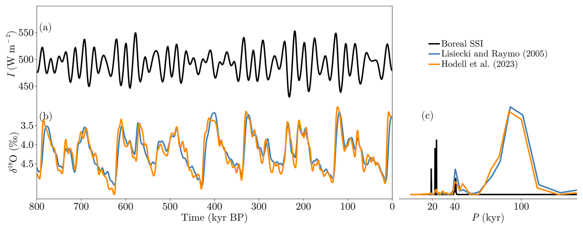
Figure 1 Time series of (a) boreal summer solstice insolation (SSI) at 65° N following Berger (1978) and Laskar et al. (2004). (b) Oxygen isotope 18 (δ¹⁸O) from Lisiecki and Raymo (2005) and Hodell et al. (2023). (c) The “100 kyr paradox” represented by the normalized periodogram for the last 800 kyr of time series shown in panels (a) and (b). All records were filtered with a low-pass Butterworth filter (cutoff frequency of 10 kyr⁻¹).

Much effort has been devoted in the last decades to investigating the mechanisms responsible for the nonlinear nature of GIV from a modeling perspective, using conceptual and comprehensive models. The underlying hypotheses of these studies are often of very different nature. Yet, most of them yield good results in terms of capturing the shape and patterns of glacial cycles as indicated by the geological record, thus making it very difficult to identify precise mechanisms (Clark et al., 2006; Imbrie et al., 2011; Paillard, 2015; Berends et al., 2021a; Verbitsky and Crucifix, 2023; Legrain et al., 2023; Ganopolski, 2024).

Within the conceptual modeling approach, much of the work done has involved mathematical models in the form of relaxation equations that reproduce GIV well. However, most of them rely on approaches that include artificial or imposed thresholds (Paillard, 1998; Paillard and Parrenin, 2004; Gildor and Tziperman, 2001; Ganopolski, 2024). Paillard (1998) presented a three-state model based on insolation and ice-volume thresholds. The underlying hypothesis was that some part of the Earth system could provide the necessary nonlinear character in order to make the climate system transition from one state to another. In particular, changes in ocean circulation were suggested to be the driver of such nonlinearity, but these were not actually captured by the model. To solve this issue, Paillard and Parrenin (2004) added an equation to the previous model that included the effect of oceanic stratification due to Antarctic sea ice and ice-sheet extension. During a glacial phase, sea ice could grow far beyond the Antarctic coasts. Through brine rejection above continental margins deep water would become saltier and denser, favoring deep water formation and stratification of the Southern Ocean and thereby CO₂ storage. In this way, CO₂ levels would decrease in the atmosphere, allowing a colder climate and the growth of the Antarctic ice sheet. When the Antarctic ice sheet reached its maximum extent at the limits of the continental shelves, sea-ice formation would occur further north and the deep water stratification would break down after a few thousand years, releasing high amounts of CO₂ that produced a glacial termination. This was suggested to be the main mechanism behind 100 kyr cycles. Gildor and Tziperman (2001) instead proposed the so-called sea-ice–temperature–precipitation feedback as the main driver of 100 kyr cycles. In this case, the growth of the sea-ice extent at the end of glacial periods would inhibit precipitation over the North American ice sheet. In this way, the mass balance would decrease, allowing for glacial terminations. As a corollary, this hypothesis suggests that 100 kyr glacial cycles result from internal oscillations of the climate system rather than from forced response to an external forcing. However, as the authors stated, many physical processes were neglected so their results did not match the records. Later on, Verbitsky et al. (2018) built a model based on dimensional analysis of ice-sheet thermodynamics. This model tried to represent the evolution of ice sheets via a linear relationship with climate temperature. When no forcing is applied, the model evolves to equilibrium. However, when forced, it reproduced different modes of rhythmicity depending on a dimensionless number (the variability number) defined as a function of eight parameters of the model. This number describes the relation between the negative and the positive feedbacks related to ice-sheet basal sliding and temperature, respectively. If this criterion is large enough, the cycles are produced every ∼ 100 kyr due to multiples of obliquity and precession cycles. This number also revealed that there is no need for nonlinear relationships in the climate or in the carbon cycle in order to produce the rhythmicity observed in the paleorecords. However, the rather general way in which it is defined does not isolate the physical mechanism that produces the glacial–interglacial oscillations. Recently, an attempt was made to build a generalized Milankovitch theory using conceptual models (Ganopolski, 2024). In this case, a model similar to that of Paillard (1998) was developed using results from the more comprehensive model CLIMBER-2 (Ganopolski and Calov, 2011). In this study, the model satisfactorily reproduced GIV, and a complete revision of the state of the art was performed. Ganopolski (2024) highlighted nonlinearities associated with ice-sheet size (increased basal velocities due to the presence of soft sediments, isostatic rebound, albedo darkening and enhanced melting due to proglacial lakes) as drivers of Pleistocene GIV.

Within the more comprehensive approach, Ganopolski and Calov (2011) employed CLIMBER-2 and investigated the role of CO₂ and dust. The authors explained the Late Pleistocene GIV as the consequence of the accumulation of dust on the surface of ice sheets, thus increasing their sensitivity and lag with respect to insolation. They concluded that 100 kyr glacial stages are created when eccentricity is small enough to allow positive ice-mass balance. When boreal summer insolation reaches high enough values (while increasing eccentricity), Northern Hemisphere ice sheets start decaying and low albedo enhances the response. In addition, they found that glacial terminations also require low CO₂ concentrations to amplify the cycles. Subsequently, Willeit et al. (2019) simulated the last 3 million years with CLIMBER-2 using multiple combined long-term simulations. The authors found that glacial cycles are a quasi-deterministic response of their model to orbital forcing since the response is robust to initial conditions. This behavior is the result of regolith removal (the erosion of soft sediments beneath the ice sheets), dust deposition and the gradual lowering of CO₂ as an imposed forcing trend. Therefore, dust was again identified as the trigger of the Late Pleistocene GIV. Later, Mitsui et al. (2023) introduced a new mechanism called vibration-enhanced synchronization (after Pikovsky et al., 2003). There, the authors revisited the Quaternary glacial cycles of their model to analyze this phenomena in detail. They found internal oscillations mainly related to dust and CO₂ feedbacks, in agreement with the conclusions of Ganopolski and Calov (2011) and Willeit et al. (2019). Thus, if the internal frequency is similar to the forcing, a frequency entrainment (or synchronization) from the external forcing is possible. Then, if the internal oscillations (found to be around 95 kyr) synchronize with the climatic precession times when the eccentricity increases (since climatic precession is modulated by eccentricity), the system oscillates at ∼ 100 kyr. However, they found that their model could be biased to glacial conditions since some deglaciations were not fully reproduced. On the other hand, Abe-Ouchi et al. (2013) used the comprehensive model IcIES-MIROC to study the role of isostatic rebound for glacial cycles. They found that the delayed response of the bedrock in the melt–elevation feedback on the ice sheets (after Oerlemans, 1980; Pollard, 1982) is a key process. They also found that ocean and dust feedbacks are not necessary and that glacial cycles are produced even with constant levels of CO₂ but that the amount of CO₂ amplifies the amplitude of the signal. Thus, the modulation of precessional cycles by eccentricity was concluded to be the driver of the 100 kyr sawtooth glacial cycles.

To summarize, in the conceptual framework we find two main problems when trying to solve Pleistocene physics: the lack of explicit physics and the need to impose ad hoc thresholds. Most models do not explicitly solve the physical processes governing climate or ice sheets and need a change in their reference states via imposed thresholds to reproduce the GIV. In turn, the comprehensive approaches provide realistic and accurate results that shed light on the likely evolution of the Earth system across the Pleistocene. However, the number of processes solved hinders the isolation of the mechanisms governing the GIV. Furthermore, despite the numerous hypotheses proposed and the wide range of model complexities employed, there is no definitive answer to the 100 kyr paradox. In this context, we have built a model with a minimal amount of explicitly resolved physical processes that successfully reproduces the GIV of the Pleistocene. Our model is an efficient and spatially averaged (we refer to this as “adimensional” since time becomes the only dimension resolved) climate–cryosphere model with explicitly solved physical processes that can be enabled or disabled independently, allowing us to isolate some of the physical processes that control the mechanisms underlying the Pleistocene records. We describe the model in Sect. 2, together with results from each model configuration. In Sect. 3 we discuss the main results. Finally, the main conclusions are summarized in Sect. 4.

2 Model description and results

Here we describe the Physical Adimensional Climate-Cryosphere mOdel (PACCO) in a progressive manner in order to provide a full picture of its capacities together with the physical basis for its formulation. PACCO represents conceptually the interaction between climate and Northern Hemisphere ice sheets using a system of up to five coupled ordinary differential equations (ODEs) as described in the following sections. The experiments summarized in Table 1 progressively capture more processes and will therefore be used as a convenient way to describe the physics captured by PACCO.

The equations governing ice-sheet dynamics are the same in all experiments. Thus, we first introduce the ice-sheet thickness H evolution as

$$\begin{array}{}\text{(1)}& {\displaystyle \frac{\mathrm{d}H}{\mathrm{d}t}}=\dot{m}-q,\end{array}$$

which is the mass conservation equation usually employed in glaciological modeling (Benn et al., 2019). $\dot{m}$ is the net surface mass balance and q is the ice discharge. The former will be described in Sect. 2.1 and the latter is

$$\begin{array}{}\text{(2)}& q=v\cdot {\displaystyle \frac{H}{L_{\mathrm{ocn}}}},\end{array}$$

where v is the ice-sheet velocity and L_ocn is the connectivity with the ocean. q increases with both v and H but is limited geographically by L_ocn. In this way, we mimic the flow of ice through the grounding line, which, in reality, only depends on the ice velocity and thickness in the oceanic boundary L_ocn. This and all other parameters of the model are listed in Table 2.

Ice velocity is decomposed into a deformation and a sliding component, respectively v_d and v_b:

$$\begin{array}{}\text{(3)}& v=v_{\mathrm{d}}+v_{\mathrm{b}}.\end{array}$$

We use Glen's flow law (Glen, 1958) to express the deformational velocity in terms of the driving stress τ_d:

$$\begin{array}{}\text{(4)}& {\mathit{v}}_{\mathrm{d}}={\displaystyle \frac{\mathrm{2}{A}_f}{n+\mathrm{2}}}\cdot H\cdot {\left|{\mathit{\tau }}_{\mathrm{d}}\right|}^{n-\mathrm{1}}\cdot {\mathit{\tau }}_{\mathrm{d}},\end{array}$$

with the usually used exponent n=3 and $A_f={\mathrm{10}}^{-\mathrm{16}}{\mathrm{Pa}}^{-\mathrm{3}}{\mathrm{yr}}^{-\mathrm{1}}$ being the Glen law flow parameter that represents the effect of the ice viscosity, which is treated as a constant. In its zero-dimensional form, Eq. (4) becomes

$$\begin{array}{}\text{(5)}& v_{\mathrm{d}}={\displaystyle \frac{\mathrm{2}}{\mathrm{5}}}\cdot A_f\cdot H\cdot {\mathit{\tau }}_{\mathrm{d}}^{\mathrm{3}}.\end{array}$$

τ_d causes ice to deform under its own weight, and it is normally expressed as

$$\begin{array}{}\text{(6)}& {\mathit{\tau }}_{\mathrm{d}}={\mathit{\rho }}_{\mathrm{ice}}\cdot g\cdot H\cdot \mathbf{\nabla }\mathit{z},\end{array}$$

where ρ_ice is the ice density (∼ 910 kg m⁻³), g is the gravitational acceleration (9.81 m s⁻²) and z is the elevation of the surface of the ice. Since PACCO is a spatially dimensionless model, the spatial derivative needs to be approximated using the typical horizontal scale of the ice sheet (L, Oerlemans, 2008; Verbitsky et al., 2018):

$$\begin{array}{}\text{(7)}& {\mathit{\tau }}_{\mathrm{d}}={\mathit{\rho }}_{\mathrm{ice}}\cdot g\cdot H\cdot {\displaystyle \frac{z}{L}}.\end{array}$$

Following Verbitsky et al. (2018), L takes a quadratic dependence on z:

$$\begin{array}{}\text{(8)}& L=c\cdot z^{\mathrm{2}},\end{array}$$

where c is a parameter that measures the slope of the ice sheet (see Table 2). In reality, this parameter depends on ice viscosity (hence on ice temperature), but for simplicity we take it as a constant. c can be estimated with the mean ice surface elevation and the ice-sheet area of a given ice sheet, taking into account that $L\sim \sqrt{S}$, with S the ice-sheet area (Verbitsky et al., 2018). This relationship is not self-limiting, but it is clear that the size of an ice sheet is bounded. Thus L is bounded between L_lb, the lower bound of the minimal possible ice sheet (Bates and Jackson, 1987), and L_ub, the upper bound of the ice-sheet scale, that is, the scale of an exemplary big ice sheet (e.g., the Antarctic or the Laurentide Ice Sheet). Both values can be obtained using the approach explained above, and their respective values can be found in Table 2.

The basal velocity field is assumed to follow a Weertman-like sliding law (Cuffey and Paterson, 2010; Pattyn, 2010; Pollard and DeConto, 2012):

$$\begin{array}{}\text{(9)}& {\mathit{v}}_{\mathrm{b}}=C\cdot \left|{\mathit{\tau }}_{\mathrm{b}}\right|\cdot {\mathit{\tau }}_{\mathrm{b}}.\end{array}$$

In the spatially adimensional simplification $C=f_{\mathrm{str}}\cdot C_{\mathrm{s}}$, this becomes

$$\begin{array}{}\text{(10)}& v_{\mathrm{b}}=f_{\mathrm{str}}\cdot C_{\mathrm{s}}\cdot {\mathit{\tau }}_{\mathrm{b}}^{\mathrm{2}},\end{array}$$

where C_s is a model parameter that represents the raw sliding coefficient derived from Pollard and DeConto (2012) and f_str is a model parameter that represents the fraction of ice streams in the ice sheet. Finally, τ_b is the basal stress that measures how easily the ice sheet slides over the underlying bedrock. It takes the expression

$$\begin{array}{}\text{(11)}& {\mathit{\tau }}_{\mathrm{b}}={\mathit{\rho }}_{\mathrm{ice}}\cdot g\cdot H\cdot \mathit{\theta },\end{array}$$

where θ is the slope of the streaming region (see Table 2, Benn et al., 2019). This quantity is set as a constant since ice streams are more or less horizontal regions due to the faster velocities they present. Therefore, τ_d and τ_b are dynamically different, since they respectively represent deformational and sliding regimes that lead to different geometries across the ice sheet.

Finally, the ice-sheet surface elevation z appearing in the previous equations is given by

$$\begin{array}{}\text{(12)}& z=H+B,\end{array}$$

with B the elevation of the bedrock that is assumed to be constant for the moment.

Table 1 Summary of the experiments performed in this work. Experiments are ordered in gradual increasing complexity.

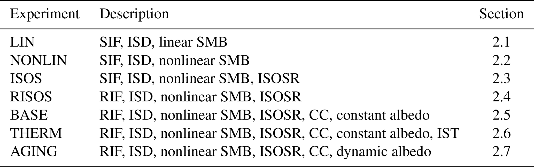
SIF: synthetic insolation forcing; RIF: real insolation forcing; ISD: ice-sheet dynamics; SMB: surface mass balance; ISOSR: isostatic response; CC: carbon cycle; IST: ice-sheet thermodynamics.

2.1 A quasi-linear configuration for surface mass balance (LIN experiment)

We start by building a simple configuration that represents the interaction between insolation and ice-sheet dynamics. PACCO receives insolation as the only forcing. For that purpose, we define a synthetic insolation forcing as a linear combination of three cosines with periods identical to those of orbital parameters (synthetic forcing and linear mass balance, LIN experiment, Table 1). Thus,

$$\begin{array}{}\text{(13)}& I=I_{\mathrm{ref}}+A_I\cdot \sum _{i=p,o}{P}_i\cdot \cos \left({\displaystyle \frac{\mathrm{2}\mathit{\pi }t}{{\mathit{\tau }}_i}}\right),\end{array}$$

where I_ref is a reference value for insolation and P_i and τ_i are the power and period associated with precession (p) and obliquity (o), respectively. We did not take into account the eccentricity because, as we explained in Sect. 1, its power in summer insolation is negligible in the present context. $A_I=\mathrm{0.5}\cdot (I_{\max }-I_{\min })$ is the amplitude of the signal, with I_min and I_max parameters based on the minimum and maximum values of the real boreal summer solstice insolation at 65° N (based on Laskar et al., 2004, after Berger, 1978). All parameter values employed are shown in Table 2. Equation (13) thus provides a synthetic insolation forcing for the model.

Insolation is then translated to sea-level temperature using an anomaly approach given by

$$\begin{array}{}\text{(14)}& T_{\mathrm{sl}}=T_{\mathrm{ref}}+A_{\mathrm{T}}\cdot \stackrel{\mathrm{‾}}{I},\end{array}$$

where T_ref is a reference value for the Earth's temperature, A_T is the amplitude of the thermal signal, and

$$\begin{array}{}\text{(15)}& \stackrel{\mathrm{‾}}{I}=\mathrm{2}\cdot {\displaystyle \frac{I-I_{\min }}{I_{\max }-I_{\min }}}-\mathrm{1}\end{array}$$

is the normalized insolation between −1 and 1. In this way we have built an extremely simple climate model. The climate response is fed into the ice sheet through the surface mass balance $\dot{m}$. This is assumed to be the only source of mass balance of the ice sheet (i.e., basal mass balance and calving are ignored), with the exception of the ice discharge (Eq. 2). Thus,

$$\begin{array}{}\text{(16)}& \dot{m}=\dot{s}-\dot{a},\end{array}$$

where the dot indicates rate of ice-mass change (m yr⁻¹); hence $\dot{s}$ is snowfall and $\dot{a}$ is ablation. Snowfall evolves linearly with the anomaly in temperature relative to a reference value T_ref. In this way it represents a linearization of the Clausius–Clapeyron equation. If the atmosphere is warmer, more moisture is allowed and vice versa (note that we assume a one-to-one equivalence of water and snow). Therefore,

$$\begin{array}{}\text{(17)}& \dot{s}={\dot{s}}_{\mathrm{ref}}+k_{\dot{s}}\cdot \left(T_{\mathrm{sl}}-T_{\mathrm{ref}}\right),\end{array}$$

with ${\dot{s}}_{\mathrm{ref}}$ and $k_{\dot{s}}$ model parameters (see Table 2). The ablation term $\dot{a}$ in Eq. (16) follows a similar approach to the positive degree day method (Braithwaite, 1980; Reeh, 1991; Ritz et al., 1996; Cuffey and Marshall, 2000; Huybrechts et al., 2004; Charbit et al., 2008; Robinson et al., 2010) that depends on the number of days in a year with sea-level temperature above the melting point. PACCO assumes a linear relationship between the ablation and the temperature anomaly and reduces the melting point constraint to T_thr. In this way, we can allow for melting at lower temperatures to account for the absence of spatial and temporal knowledge. We then define ablation as

$$\begin{array}{}\text{(18)}& \dot{a}=\mathit{\lambda }\cdot \left(T_{\mathrm{sl}}-T_{\mathrm{thr}}\right).\end{array}$$

Here, λ is a parameter that transfers temperature anomaly to ice-mass loss. Note that both $\dot{s}$ and $\dot{a}$ are defined as strictly positive.

Verbitsky et al. (2018)Pollard and DeConto (2012)Margold et al. (2015)Margold et al. (2015)Bates and Jackson (1987)Cuffey and Paterson (2010)Willeit and Ganopolski (2018)Benn et al. (2019)Willeit and Ganopolski (2018)Le Meur and Huybrechts (1996)Payne et al. (2004); Nick et al. (2009)

Table 2 Model parameters. Note that the parameters not referenced correspond to model calibration values.

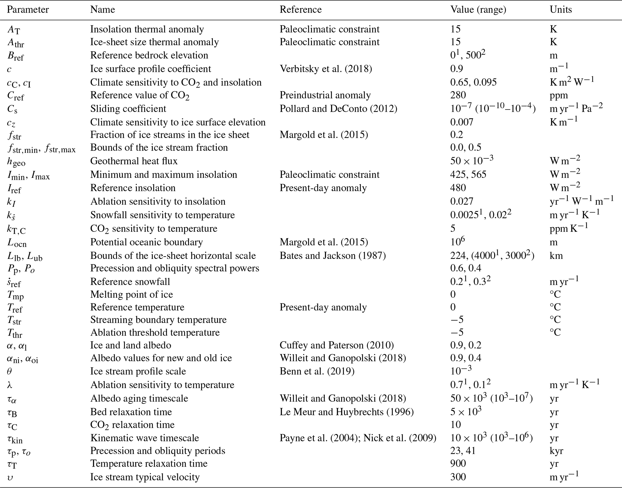
¹ Calibration value for LIN, NONLIN, ISOS and RISOS experiments. ² Calibration value for BASE, THERM and AGING experiments.

The model structure and flowchart are described in Fig. 2. This configuration essentially consists of a linear relation between insolation and mass balance and a nonlinear one between ice thickness and velocity. As expected, when integrating over 800 kyr (Fig. 3 shows the simulations performed using different values of the sliding parameter C_s), glacial inceptions and deglaciations respectively occur shortly after insolation minima and maxima, with a pattern that resembles the sawtooth observed in proxy records. Interestingly, the power spectrum of the response of H and v presents a peak around periodicities of 60 kyr, which is, however, absent from the forcing. This is a manifestation of the nonlinearities introduced by the ice dynamics and is a consequence of the fact that certain interglacials are very long, since the system evolves explicitly with insolation and only those insolation minima below a certain threshold allow for a positive mass balance, leading to an increase in the ice mass. In short, the ice-sheet dynamics creates a certain degree of nonlinearity that appears, however, to be not powerful enough to allow for a realistic GIV simulation.

Figure 2 LIN experiment scheme. Note the linear relationship between the forcing and the evolution of the ice thickness. This configuration employs Eqs. (1), (13), (17) and (18).

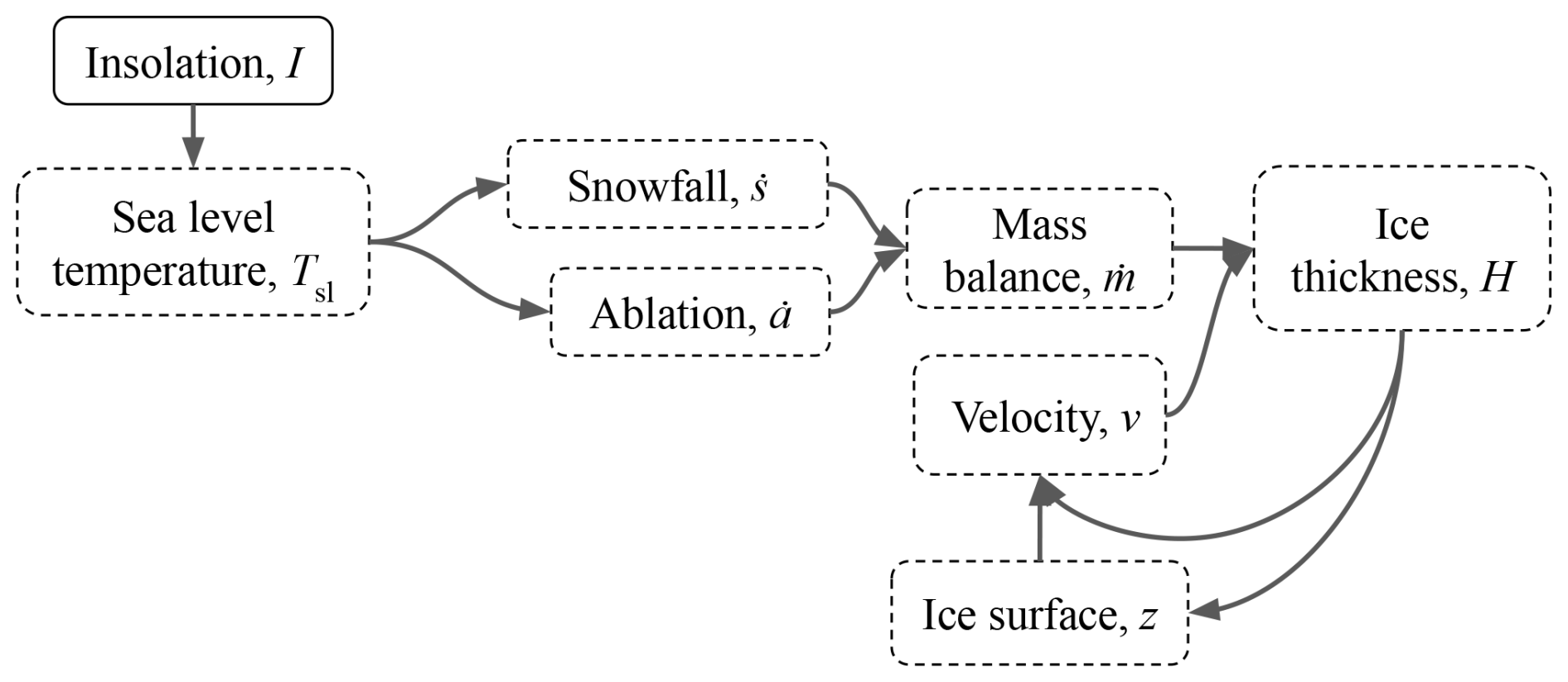
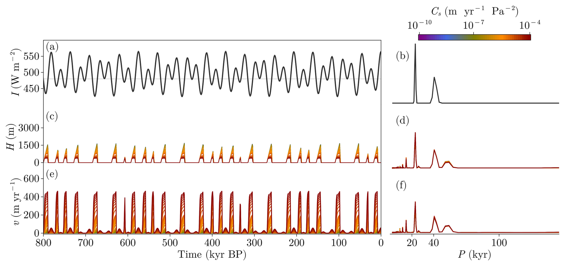
Figure 3 Results of the LIN simulation. (a, c, e) Time series obtained from the model using different sliding factors C_s. (b, d, f) Normalized periodograms obtained from the time series in the left column. Note that when normalizing spectra, series were cut off for periods larger than 200 kyr.

2.2 Introducing feedbacks on surface mass balance (NONLIN experiment)

In order to build a more physically motivated model, important feedbacks must be included. The melt–elevation feedback (Weertman, 1961; Clark and Pollard, 1998; Oerlemans, 2003) is known to be a fundamental process controlling ice-sheet accumulation and ablation. This feedback accelerates melting under a shrinking ice sheet and limits ablation when the ice sheet is growing, leading to hysteresis in the ice sheet's volume with respect to temperature (Robinson et al., 2012; Garbe et al., 2020). To take this feedback into account, the mass balance equations are modified by using T_surf instead of T_sl, where

$$\begin{array}{}\text{(19)}& T_{\mathrm{surf}}=T_{\mathrm{sl}}-\mathrm{\Gamma }\cdot z\end{array}$$

and

$$\begin{array}{}\text{(20)}& {\displaystyle }\dot{s}={\dot{s}}_{\mathrm{ref}}+k_{\dot{s}}\cdot \left(T_{\mathrm{surf}}-T_{\mathrm{ref}}\right),\text{(21)}& {\displaystyle }\dot{a}=\mathit{\lambda }\cdot \left(T_{\mathrm{surf}}-T_{\mathrm{thr}}\right),\end{array}$$

where Γ=0.0065 K m⁻¹ is the atmospheric lapse rate for polar regions. Introducing the melt–elevation feedback in the mass balance (NONLIN, Table 1, Fig. 4) clearly alters the response to the forcing (Fig. 5). If the ice sheet is dynamic enough (i.e., high values of the sliding factor C_s), the model resonates to certain multiples of the insolation fundamental periods. This means that the elevation feedback introduces a nonlinearity via the modulation of the height amplitude, which increases the inertia of the system (Abe-Ouchi et al., 2013). Thus, we distinguish two regimes: those with fast, insolation-driven ice sheets (high C_s) and those with slow, climate–cryosphere-driven ice sheets (low C_s). Therefore, as in the previous formulation (LIN), periodicities of 60 kyr can be found, but also 80, 100 and 120 kyr peaks now emerge. Still, this phenomenon does not produce a dominant GIV periodicity of 100 kyr.

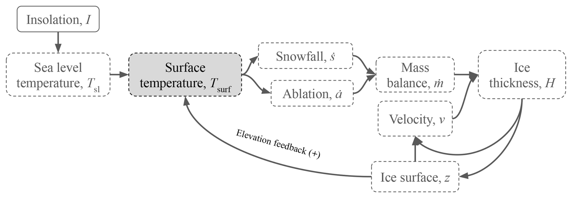
Figure 4 NONLIN experiment scheme. The previously linear relationship between the forcing and the evolution of the ice thickness (LIN) is now nonlinear due to the elevation feedback. Model additions with respect to LIN are highlighted in gray. This configuration employs Eqs. (1), (13), (20) and (21).

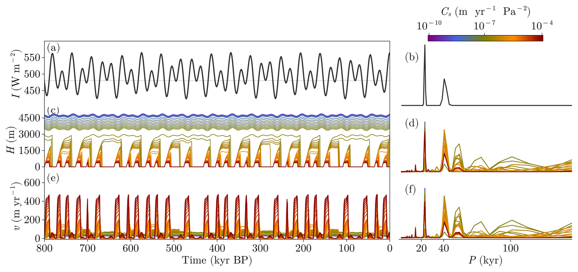
Figure 5 Results of the NONLIN simulation. (a, c, e) Time series obtained from the model using different sliding factors C_s and (b, d, f) associated normalized periodograms. Note that when normalizing spectra, series were cut off for periods larger than 200 kyr.

2.3 Delayed isostatic adjustment (ISOS experiment)

Changes in ice load lead to delayed vertical bedrock motion, a process commonly known as isostatic adjustment (ISOS experiment, Table 1). This effect is included here via another prognostic variable in the model (Fig. 6), such that the bedrock elevation B evolves according to

$$\begin{array}{}\text{(22)}& {\displaystyle \frac{\mathrm{d}B}{\mathrm{d}t}}={\displaystyle \frac{\left[B_{\mathrm{ref}}-\frac{{\mathit{\rho }}_{\mathrm{ice}}}{{\mathit{\rho }}_{\mathrm{bed}}}\cdot H\right]-B}{{\mathit{\tau }}_{\mathrm{B}}}},\end{array}$$

where B_ref is a model parameter representing the Earth surface elevation in the absence of load, ρ_bed is the bedrock density (∼ 2700 kg m⁻³) and τ_B is the relaxation time of the bed (see Table 2). In this way, when the ice starts to grow, the bed converges exponentially towards an isostatic equilibrium between the ice column and the displaced mantle material (Saltzman, 2001). Figure 7 shows, as in previous cases, the results of a simulation for different levels of the sliding factor C_s. Resonance of the system to longer periods is favored for the less dynamic runs (lowest C_s values). Reaching a glacial termination is now facilitated by the fact that ablation is greater than accumulation at low elevations (Fig. 8). We can define an elevation threshold z_thr such that when z≤z_thr (i.e.,  z is located below the red curve in Fig. 8) ablation is surpassed by accumulation. In other words, z_thr represents the equilibrium line altitude in the ice sheet:

$$\begin{array}{}\text{(23)}& z_{\mathrm{thr}}={\displaystyle \frac{{\dot{s}}_{\mathrm{ref}}+k_{\dot{s}}\cdot \left(T_{\mathrm{sl}}-T_{\mathrm{ref}}\right)-\mathit{\lambda }\cdot \left(T_{\mathrm{sl}}-T_{\mathrm{thr}}\right)}{\left(k_{\dot{s}}-\mathit{\lambda }\right)\cdot \mathrm{\Gamma }}}.\end{array}$$

This happens more easily for the ISOS experiments since the simulated ice-sheet heights are generally lower for the same set of parameters, as a consequence of the bedrock depression induced by the ice load. Thus, isostasy favors glacial terminations, and 100 kyr cycles can now more clearly emerge for certain values of the sliding factor. We must bear in mind, however, that so far our insolation forcing is synthetic. We therefore next turn to a more realistic forcing to assess whether this formulation allows for a good match with paleodata.

Figure 6 ISOS experiment scheme. Note that the surface elevation feedback is altered due to bedrock response. Model additions with respect to NONLIN are highlighted in gray. This configuration employs Eqs. (1), (13), (20), (21) and (22).

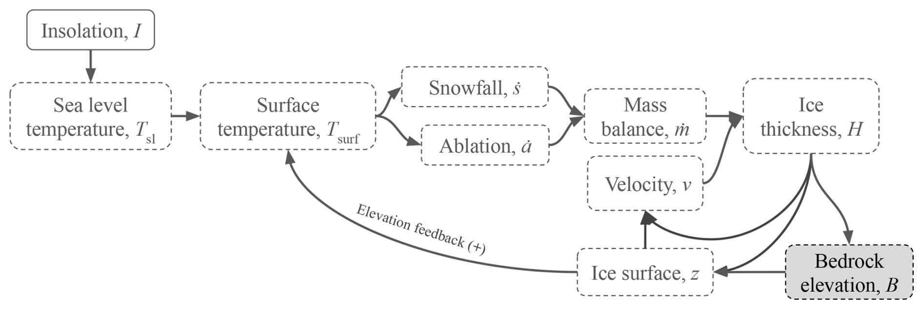
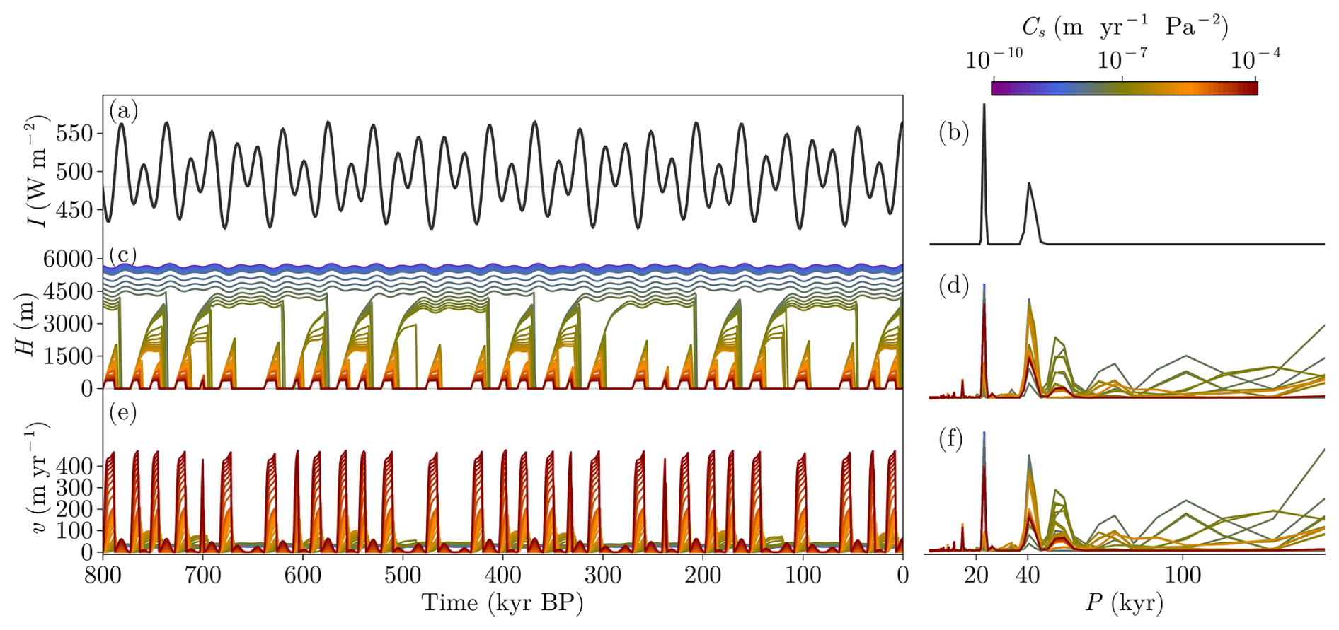
Figure 7 Results from the ISOS simulation. (a, c, e) Time series obtained from the model using different sliding factors C_s and (b, d, f) associated normalized periodograms. Note that when normalizing spectra, series were cut off for periods larger than 200 kyr.

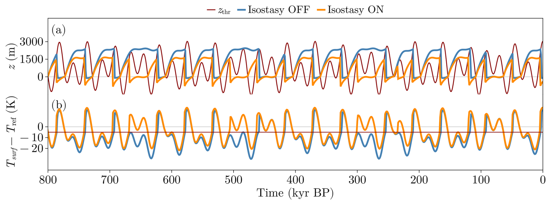
Figure 8 Time series for (a) ice surface elevation z (blue, orange) and z_thr (red) and (b) surface temperature anomaly (with respect T_ref). z_thr is the point where $\dot{a}$ surpasses $\dot{s}$, and the horizontal red line indicates T_thr, which is the isoline where $\dot{a}$ becomes positive. Note that the plotted curves are for the same sliding factor $C_{\mathrm{s}}=\mathrm{4}\times {\mathrm{10}}^{-\mathrm{7}}$ m yr⁻¹ Pa⁻².

2.4 ISOS configuration with real insolation (RISOS experiment)

To answer if the only missing piece to reproduce GIV is the shape of the forcing, we perform the RISOS experiment with the ISOS configuration (Table 1, Fig. 6) but using the boreal summer solstice insolation at 65° N (Fig. 9) as forcing I (obtained following Berger, 1978; Laskar et al., 2004). The model produces resonance at higher periodicities than those corresponding to obliquity and precession, so glacial terminations occur at different multiples of the former, depending on the sliding intensity (Fig. 9). However, the simulated timing does not yet match that provided by paleoclimatic proxies. The model response is still quite linear with the insolation forcing, so the amplitude of some of its peaks is not enough to make the ice sheet deglaciate for low sliding. On the contrary, a moderate increase in insolation easily induces a termination for high sliding. The absence of a satisfactory synchronization with the observed deglaciations, even for mid-range values of the sliding factor, likely indicates that the model still lacks some important climatic processes. These will be addressed in the next section.

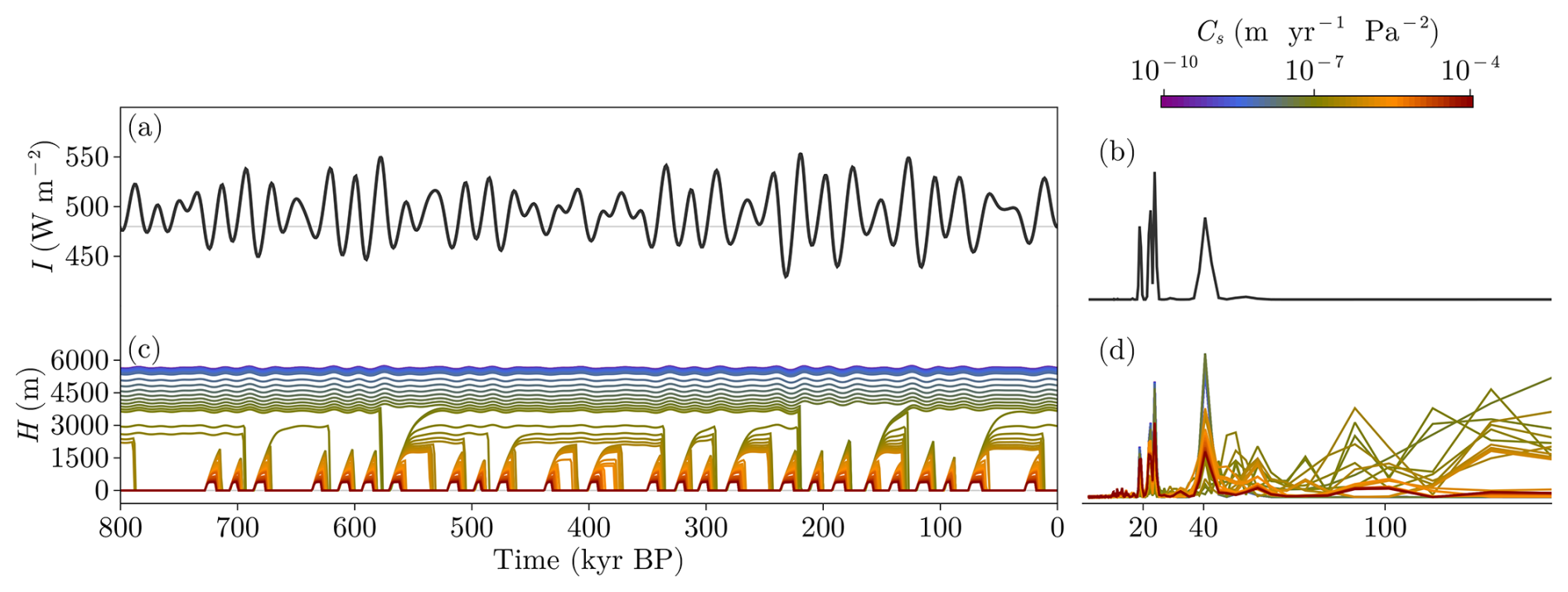
Figure 9 Results of the RISOS simulation. (a, c, e) Time series obtained from the model using different sliding factors C_s. (b, d, f) Normalized periodograms obtained from the time series in the left column. Note that when normalizing spectra, series were cut off for periods larger than 200 kyr.

2.5 Improving the coupling between ice sheet and climate (BASE experiment)

The first required improvement concerns the treatment of air temperature in the model, which is now regionalized in order to include the two-way interaction between the atmosphere and the cryosphere, as well as its response to the radiative forcing (Table 1). The regional air temperature T hence evolves in time as follows:

$$\begin{array}{}\text{(24)}& {\displaystyle \frac{\mathrm{d}T}{\mathrm{d}t}}={\displaystyle \frac{\left[T_{\mathrm{ref}}+c_{\mathrm{I}}\cdot R_{\mathrm{I}}+c_{\mathrm{C}}\cdot R_{\mathrm{C}}-c_z\cdot z\right]-T}{{\mathit{\tau }}_{\mathrm{T}}}},\end{array}$$

with c_I, c_C and c_Z the climate sensitivities to insolation, atmospheric CO₂ radiative forcing and ice-sheet height, respectively, and τ_T the thermal characteristic time. In this way, positive anomalies in insolation or atmospheric CO₂ concentration C tend to increase temperature, while the ice-sheet size tends to decrease it. Note that the local effect of T_surf is now translated to a more regional effect via T, which is affected by the carbon cycle and the size of the Northern Hemisphere ice sheets. Finally, R_I and R_C are the radiative forcing associated with I and C, respectively defined as

$$\begin{array}{}\text{(25)}& R_{\mathrm{I}}=I-I_{\mathrm{ref}}\end{array}$$

and

$$\begin{array}{}\text{(26)}& R_{\mathrm{C}}=\mathrm{5.35}\cdot \log \left({\displaystyle \frac{C}{C_{\mathrm{ref}}}}\right).\end{array}$$

The latter was formulated by Myhre et al. (1998), and it is commonly employed in conceptual modeling. Here C_ref is a reference value for carbon dioxide (typically set to the preindustrial value of 280 ppm) and

$$\begin{array}{}\text{(27)}& {\displaystyle \frac{\mathrm{d}C}{\mathrm{d}t}}={\displaystyle \frac{\left[C_{\mathrm{ref}}+k_{\mathrm{T},\mathrm{C}}\cdot \left(T-T_{\mathrm{ref}}\right)\right]-C}{{\mathit{\tau }}_{\mathrm{C}}}},\end{array}$$

where k_T,C is a parameter that translates the anomaly in temperature into changes in the concentration of carbon dioxide. This reflects the capability of the sources and sinks of atmospheric CO₂ to vary with temperature.

Another improvement in the model is the ablation term that now follows an ITM-like parameterization (insolation temperature melting method, Pellicciotti et al., 2005; Van Den Berg et al., 2008; Robinson et al., 2010),

$$\begin{array}{}\text{(28)}& \dot{a}=k_{\mathrm{I}}\cdot \left(\mathrm{1}-\mathit{\alpha }\right)\cdot \left(I-I_{\mathrm{ref}}\right)+\mathit{\lambda }\cdot \left(T-T_{\mathrm{thr}}\right),\end{array}$$

where k_I is the sensitivity of ablation to shortwave radiation (insolation) and α is the system albedo (see Table 2). If there is no ice we impose α=α_l, which is the value of land albedo. This improvement was made in order to take into account both shortwave and longwave radiation. As mentioned before, since ice surface elevation is already included in Eq. (24), ablation and snowfall use T instead of T_surf:

$$\begin{array}{}\text{(29)}& \dot{s}={\dot{s}}_{\mathrm{ref}}+k_{\dot{s}}\cdot \left(T-T_{\mathrm{ref}}\right).\end{array}$$

This model configuration is now represented in Fig. 10, and the results of sensitivity experiments to different C_s values are shown in Fig. 11. The sliding strength modulates the amplitude of the ice thickness and thus the ice-sheet sensitivity to full deglaciation. With this, we produce a more realistic 100 kyr periodicity in H than in RISOS when also using real insolation forcing. However, the timing and periodicity of T are not satisfactory yet, suggesting the nonlinear response of the model is still too weak to produce reliable GIV.

Figure 10 BASE experiment scheme. Model additions with respect to ISOS are highlighted in gray. This configuration employs Eqs. (1), (22), (24), (27), (28) and (29).

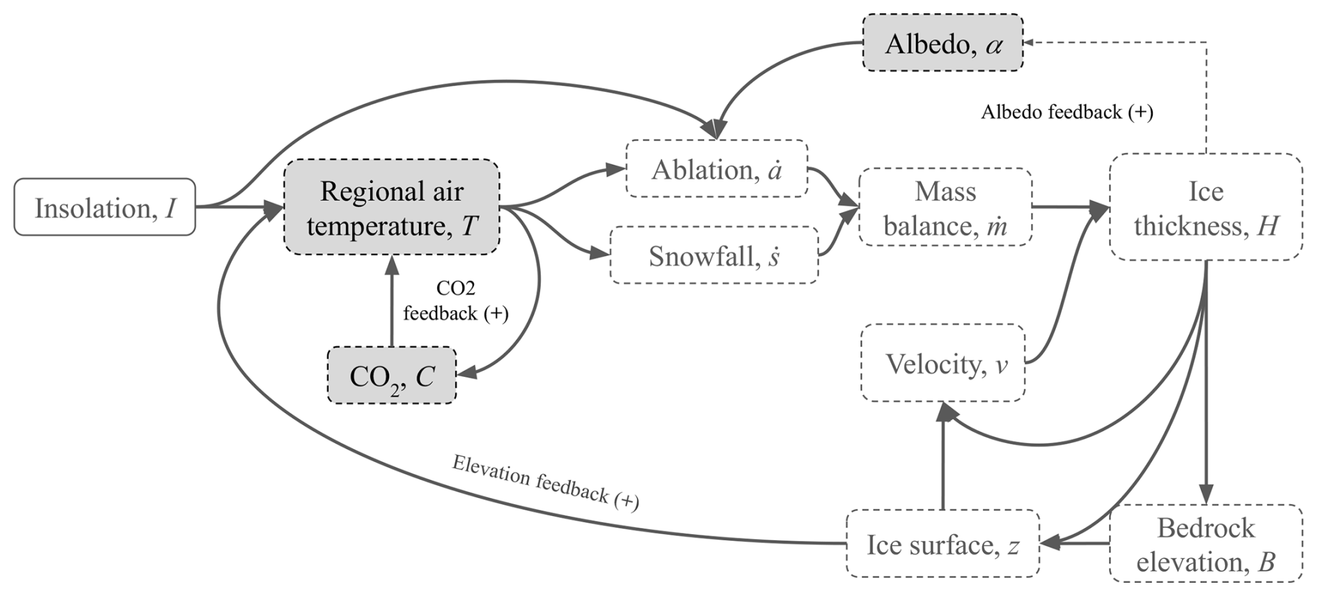
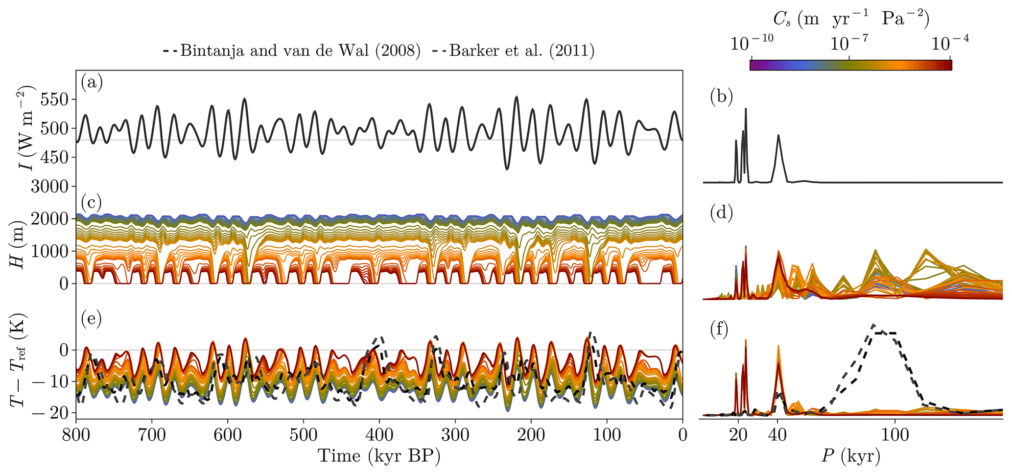
Figure 11 Results of the BASE simulation. (a, c, e) Time series obtained from the model using different sliding factors C_s. (b, d, f) Normalized periodograms obtained from the time series in the left column. Note that when normalizing spectra, series were cut off for periods larger than 200 kyr. Note that in panels (e) and (f) dashed lines refer to two different proxies.

Based on the literature, there are at least two other ways (Ganopolski, 2024) to amplify the model's nonlinear behavior: through ice-sheet thermodynamics and through ice darkening. Both will be investigated in the next section as possible sources of improved GIV accuracy.

2.6 Ice-sheet thermodynamics (THERM experiment)

One way to enhance the nonlinear response of the system is via ice-sheet thermodynamics and its effect on the basal sliding and streaming potential of the ice sheet (i.e., following the thermodynamic hypothesis, Verbitsky et al., 2018; Ganopolski, 2024, Table 1). The temperature of the base of an ice sheet (T_ice) is influenced by both ice insulation and ice creep. If basal temperature reaches the pressure melting point, basal sliding is enhanced and ice streams accelerate and expand further. To parameterize this process we consider the interaction between a cold and a temperate environment, the air and the bed, respectively. At the base,

$$\begin{array}{}\text{(30)}& \mathrm{d}Q={\mathit{\rho }}_{\mathrm{ice}}\cdot S\cdot H_{\mathrm{b}}\cdot c_{\mathrm{ice}}\cdot \mathrm{d}{T}_{\mathrm{ice}},\end{array}$$

with c_ice=2009 J kg⁻¹ K⁻¹ the ice specific heat capacity, S the ice surface, and H_b the thickness of the bottom boundary layer in which output and input heat fluxes affect the basal dynamics of the ice sheet (Verbitsky et al., 2018). This boundary can be redefined using the ratio between advective and diffusive transport (the Péclet number, Pe) as $H_{\mathrm{b}}={\mathit{Pe}}^{-\mathrm{1}/\mathrm{2}}\cdot H$ (Verbitsky et al., 2018). If we additionally divide by the time step and S, we get an equation for the evolution in time of the basal ice temperature T_ice:

$$\begin{array}{}\text{(31)}& {\displaystyle \frac{\mathrm{d}{T}_{\mathrm{ice}}}{\mathrm{d}t}}={\displaystyle \frac{{\mathit{Pe}}^{\mathrm{1}/\mathrm{2}}}{c_{\mathrm{ice}}\cdot {\mathit{\rho }}_{\mathrm{ice}}\cdot H}}\cdot h,\end{array}$$

with h the sum of the different heat fluxes between the temperate and cold environments. Now, we will define the different components. The bed of an ice sheet (temperate environment) is exposed to the geothermal heat flux h_geo from the lithosphere, here taken to be a constant parameter (see Table 2), and to the frictional heat production due to basal drag:

$$\begin{array}{}\text{(32)}& h_{\mathrm{drag}}=v_{\mathrm{b}}\cdot {\mathit{\tau }}_{\mathrm{b}}.\end{array}$$

These two terms act as a heat source to the ice sheet through its base. The counteracting part are the terms that extract heat from the boundary layer. At the air–ice interface (cold environment) there is heat loss due to ice conduction (h_cond):

$$\begin{array}{}\text{(33)}& h_{\mathrm{cond}}=-k_{\mathrm{T}}\cdot \mathrm{\nabla }{T}_{\mathrm{ice}},\end{array}$$

with $k_{\mathrm{T}}=\mathrm{2.1}\mathrm{W}{\mathrm{m}}^{-\mathrm{1}}{\mathrm{K}}^{-\mathrm{1}}$ the ice thermal conductivity (Huybrechts et al., 1996). Note that we have neglected advection in both the horizontal and the vertical dimensions since the former is assumed to be zero when treating the entire ice sheet and the latter is negligible in the heat balance ($\sim {\mathrm{10}}^{-\mathrm{6}}\mathrm{W}{\mathrm{m}}^{-\mathrm{2}}$). Equation (33) relies on the assumption that conduction can be defined across the ice column (assumed to be an isotropic medium) as

$$\begin{array}{}\text{(34)}& h_{\mathrm{cond}}=k_{\mathrm{T}}\cdot {\displaystyle \frac{T-T_{\mathrm{ice}}}{H\cdot \left(\mathrm{1}-{\mathit{Pe}}^{-\mathrm{1}/\mathrm{2}}\right)}}.\end{array}$$

In the ice sheet, the advection of cold ice from the surface due to snowfall accumulation cools down the base. Hence, an advective term h_adv can be defined using a typical vertical velocity scale given by $\dot{s}$ (Verbitsky et al., 2018):

$$\begin{array}{}\text{(35)}& h_{\mathrm{adv}}=c_{\mathrm{ice}}\cdot {\mathit{\rho }}_{\mathrm{ice}}\cdot \dot{s}\cdot {\displaystyle \frac{T-T_{\mathrm{ice}}}{{\mathit{Pe}}^{\mathrm{1}/\mathrm{2}}-\mathrm{1}}}.\end{array}$$

where c_ice=2009 J kg⁻¹ K⁻¹ is the ice specific heat. Finally, by definition, the Péclet number is the ratio between the diffusive and the advective transport rates. Thus, in PACCO,

$$\begin{array}{}\text{(36)}& \mathit{Pe}={\displaystyle \frac{H}{k_{\mathrm{T}}}}\cdot c_{\mathrm{ice}}\cdot {\mathit{\rho }}_{\mathrm{ice}}\cdot \dot{s},\end{array}$$

where we removed the dependence on H_b since it entails a second-order variation on the heat fluxes.

Once the thermodynamics are defined, the effect on ice-sheet dynamics is translated through the fraction of ice streams f_str within the ice sheet, which evolves in time according to

$$\begin{array}{}\text{(37)}& {\displaystyle \frac{\mathrm{d}{f}_{\mathrm{str}}}{\mathrm{d}t}}={\displaystyle \frac{f_{\mathrm{str},\mathrm{ref}}-f_{\mathrm{str}}}{{\mathit{\tau }}_{\mathrm{kin}}}},\end{array}$$

with ${\mathit{\tau }}_{\mathrm{kin}}=L\cdot v_{\mathrm{kin}}^{-\mathrm{1}}$ the time that an ice stream needs to propagate into the interior of the ice sheet (Nye, 1963; Jóhannesson et al., 1989; Payne et al., 2004; Nick et al., 2009). In this way, we account for the fact that the entire ice-sheet base does not become temperate at once but rather gradually with a characteristic time τ_kin. The reference value of streaming f_str,ref depends explicitly on the thermodynamics:

$$\begin{array}{}\text{(38)}& f_{\mathrm{str},\mathrm{ref}}=\left(f_{\mathrm{str},\max }-f_{\mathrm{str},\min }\right)\cdot p_{\mathrm{c}}+f_{\mathrm{str},\min },\end{array}$$

where f_str,max and f_str,min are model parameters based on glaciological constraints, and p_c is the propagation coefficient,

$$\begin{array}{}\text{(39)}& p_{\mathrm{c}}={\displaystyle \frac{T_{\mathrm{ice}}-T_{\mathrm{str}}}{T_{\mathrm{mp}}-T_{\mathrm{str}}}}.\end{array}$$

Here, T_mp is the ice melting point temperature (0 °C) and T_str the temperature boundary that allows streaming propagation; p_c is a number between 0 and 1 that accounts for the state of the base. If T_ice≤T_str, p_c=0 and $f_{\mathrm{str},\mathrm{ref}}=f_{\mathrm{str},\min }$ are imposed since the base is frozen. If, on the contrary, T_ice>T_str, the base starts to be temperate. Thus, $\mathrm{0}<p_{\mathrm{c}}\le \mathrm{1}$ and $f_{\mathrm{str},\min }<f_{\mathrm{str},\mathrm{ref}}\le f_{\mathrm{str},\max }$. At this point, the ice sheet will tend via Eq. (37) to present more streaming and basal sliding. We limit p_c to 1 and $f_{\mathrm{str},\mathrm{ref}}=f_{\mathrm{str},\max }$. As a summary, this model configuration accounts for the warming at the base of the entire ice sheet (Eqs. 31 and 37).

Figure 12 THERM experiment scheme. Model additions with respect to BASE are highlighted in gray. This configuration employs Eqs. (1), (22), (24), (27), (28), (29) and (31).

Since this configuration tends to enhance the nonlinearities associated with basal dynamics, we first carried out a brief experiment to test from which scale of sliding sensitivity (C_s) the model starts reacting (Fig. A1). We saw that two regimes are produced: one produces deglaciations but the other one remains in a state with no glacial terminations. Thus, a value above 10⁻⁶ m yr⁻¹ Pa⁻² is needed to allow GIV. Then a sensitivity experiment with respect to τ_kin was carried out (Fig. 13) fixing $C_{\mathrm{s}}=\mathrm{5}\times {\mathrm{10}}^{-\mathrm{6}}$ m yr⁻¹ Pa⁻² since it allows a maximum ice-sheet elevation that cools the atmosphere to the mean value of the proxies (Fig. 13a). As can be seen, if τ_kin is above GIV timescales (>100 kyr), the streaming propagation takes too much time and does not increase the total basal dynamics enough to allow deglaciations. On the contrary, lower τ_kin (blue tones in Fig. 13) produce glacial terminations. Thanks to the introduction of enhanced ice dynamics through the addition of basal velocities dependent on ice thermodynamics, the THERM configuration facilitates the occurrence of response periods longer than that of the forcing. Therefore, THERM configuration improves the results compared to BASE configuration. This is supported by the findings of other studies (e.g., Verbitsky et al., 2018) that successfully capture GIV using a thermodynamic mechanism. However, the match with paleoclimatic proxies is still improvable in our model.

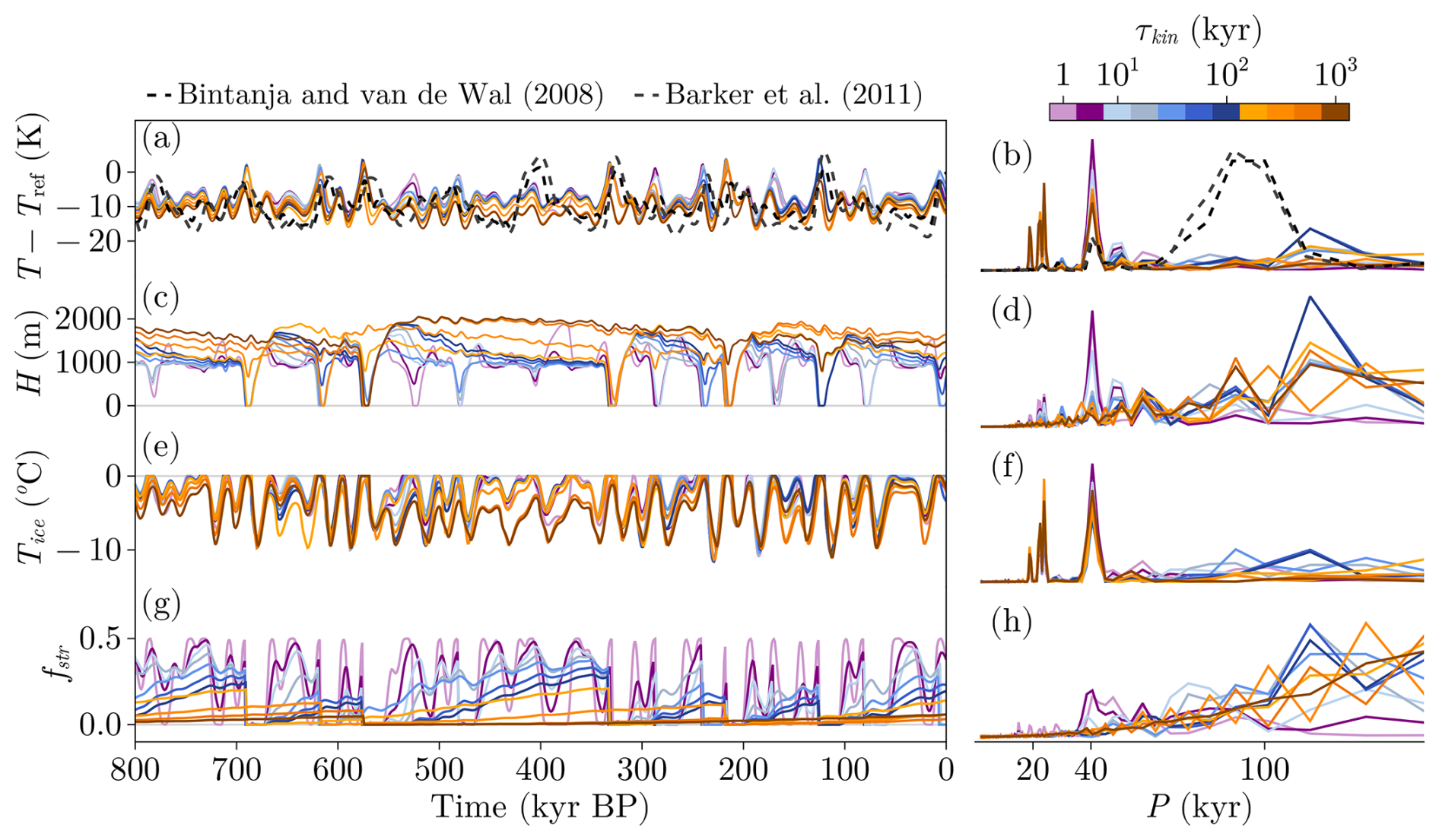
Figure 13 Results of the THERM simulation using $C_{\mathrm{s}}=\mathrm{5}\times {\mathrm{10}}^{-\mathrm{6}}$ m yr⁻¹ Pa⁻². (a, c, e, g) Time series obtained from the model using different τ_kin (colors). (b, d, f, h) Normalized periodograms obtained from the time series in the left column. Note that when normalizing spectra, series were cut off for periods larger than 200 kyr.

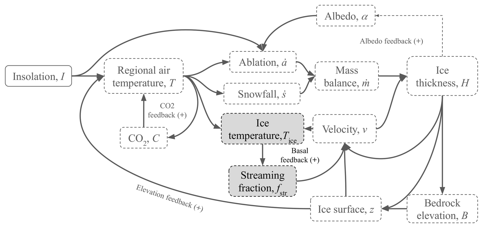
2.7 Ice aging (AGING experiment)

Another way of amplifying the nonlinear response of the Earth system to insolation forcing is through the reduction in ice albedo due to its natural darkening and dust deposition (Ganopolski and Calov, 2011; Willeit and Ganopolski, 2018; Willeit et al., 2019; Ganopolski, 2024, Table 1). The former is related to the compaction of snow, and the latter is due to the aridity of glacial landscapes, which favors the deposition of dust on ice sheets. These phenomena can be easily implemented in PACCO via a diagnostic equation for the albedo α:

$$\begin{array}{}\text{(40)}& \mathit{\alpha }={\mathit{\alpha }}_{\mathrm{ni}}-{\displaystyle \frac{{\mathit{\alpha }}_{\mathrm{ni}}-{\mathit{\alpha }}_{\mathrm{oi}}}{{\mathit{\tau }}_{\mathit{\alpha }}}}\cdot A,\end{array}$$

with τ_α the relaxation time associated with the change in albedo for the entire ice sheet. A is the ice age that depends on the presence or absence of ice. The minimum and maximum values of α are α_ni and α_oi, which are the estimated albedo values of fresh snow/new ice and old and dirty ice, respectively. Again, if there is no ice, we impose α=α_l. Accordingly, α therefore evolves in time when there is ice. In this manner, if the ice is maintained long enough, its decreasing albedo results in a nonlinear increase in ablation. However, the assumption that aging affects the entire ice sheet is a crude one, since accumulation areas are covered by fresh snow, and, therefore, their contribution to ablation must be smaller. Thus, we add an additional constraint:

$$\begin{array}{}\text{(41)}& \mathit{\alpha }={\mathit{\alpha }}_{\mathrm{ni}}\mathrm{if}\dot{m}>\mathrm{0}.\end{array}$$

In this way, if snowfall outweighs ablation, we assume that ablation zones are covered by snow (with snow/new ice albedo, α_ni), but if ablation is higher than snowfall, darker ice is exposed. In this way, the mass balance sees the time-evolving value of albedo. The result is the model configuration represented in Fig. 14.

Figure 14 AGING experiment scheme. Model additions with respect to BASE are highlighted in gray. This configuration employs Eqs. (1), (22), (24), (27), (28), (29) and (40).

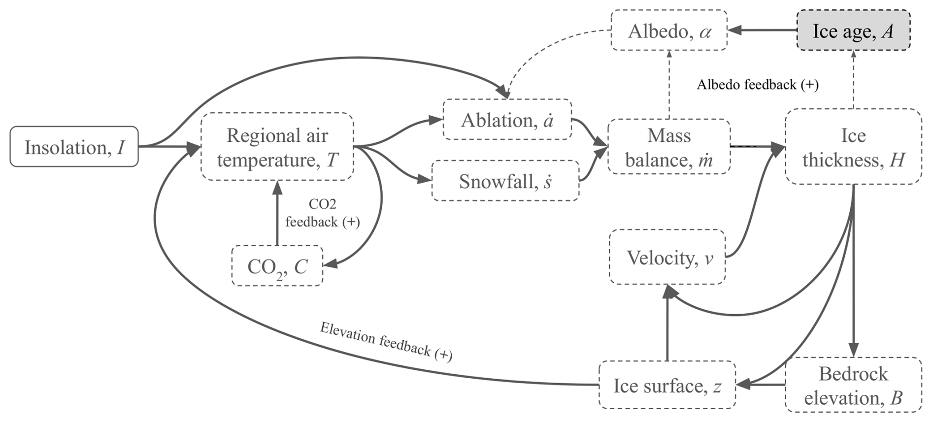
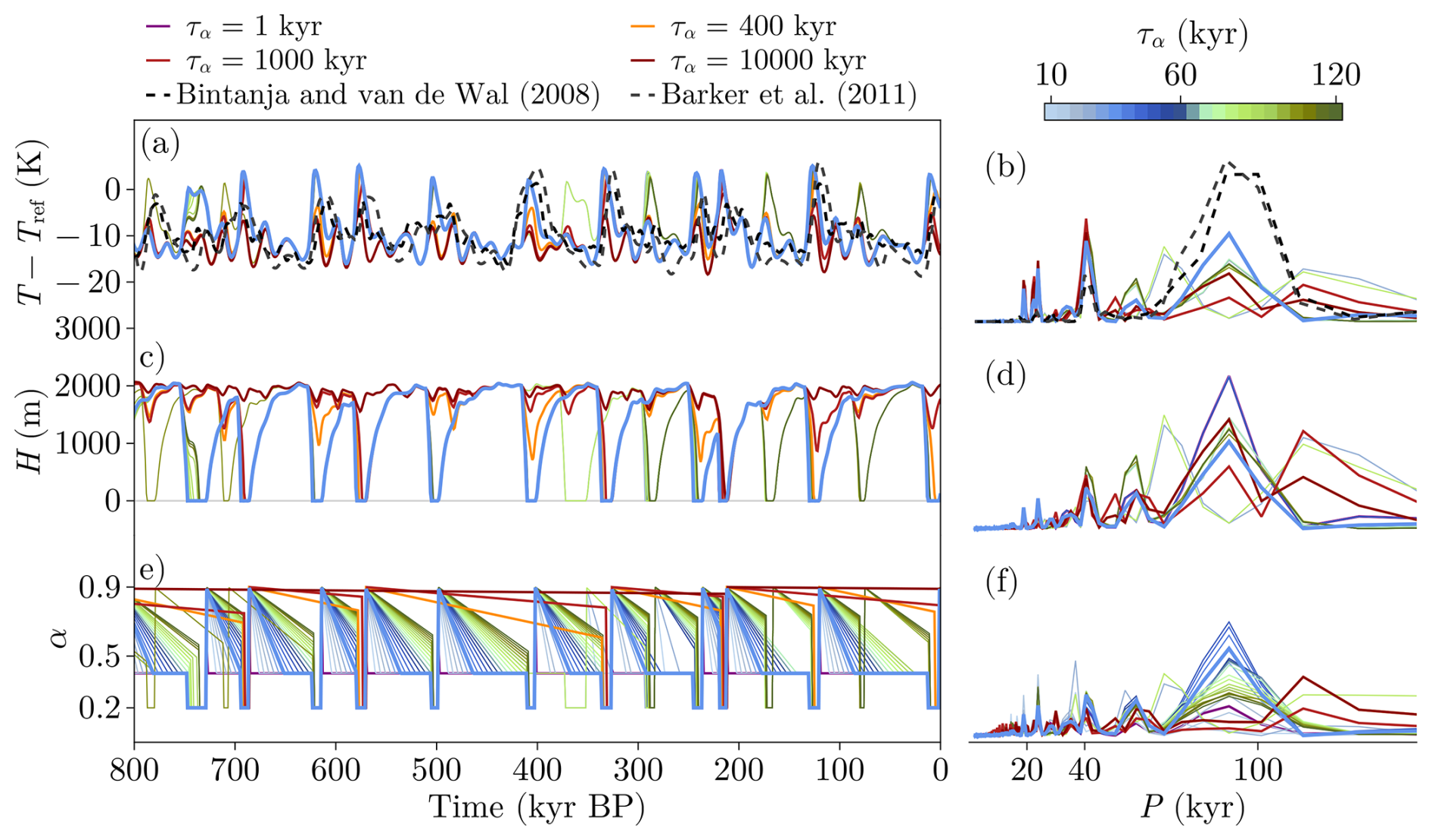
Figure 15 Results of the AGING simulation. (a, c, e) Time series obtained from the model using different aging times τ_α. (b, d, f) Normalized periodograms obtained from the time series in the left column. We use a color bar for a range of periodicities in the GIV interval (10–120 kyr, from blue to green colors) and add some extreme values (1, 400, 1000, 10 000 kyr), represented by lines with red shadings. Note that when normalizing spectra, series were cut off for periods larger than 200 kyr.

Sensitivity experiments with respect to the sliding factor C_s show that a value from 10⁻¹⁰ to 10⁻⁷ (range from  Pollard and DeConto, 2012) produces GIV-like oscillations (Fig. A2). Thus, we fixed the value of C_s to $\mathrm{0.3}\times {\mathrm{10}}^{-\mathrm{7}}$ since this sensitivity modulates ice-sheet size to one that cools the atmosphere to the proxy levels. A low level of this parameter is also supported by the idea that Late Pleistocene ice sheets were slow (Berends et al., 2021a, Fig. A2). A realization for different values of τ_α is given in Fig. 15. Our results show that the aging process is relevant to reproduce the GIV. However, its particular value is not that important since there is some clustering in Fig. 15 between non-deglacial and deglacial regimes. In this experiment, values below 60 kyr seem to provide a good representation of the Late Pleistocene since they provide high spectral power around 100 kyr and a good agreement with proxies. Thus, we will fix τ_α=50 kyr and $C_{\mathrm{s}}=\mathrm{0.3}\times {\mathrm{10}}^{-\mathrm{7}}\mathrm{m}{\mathrm{yr}}^{-\mathrm{1}}{\mathrm{Pa}}^{-\mathrm{2}}$ to compare the rest of the states of this model run with different proxies (Fig. 16).

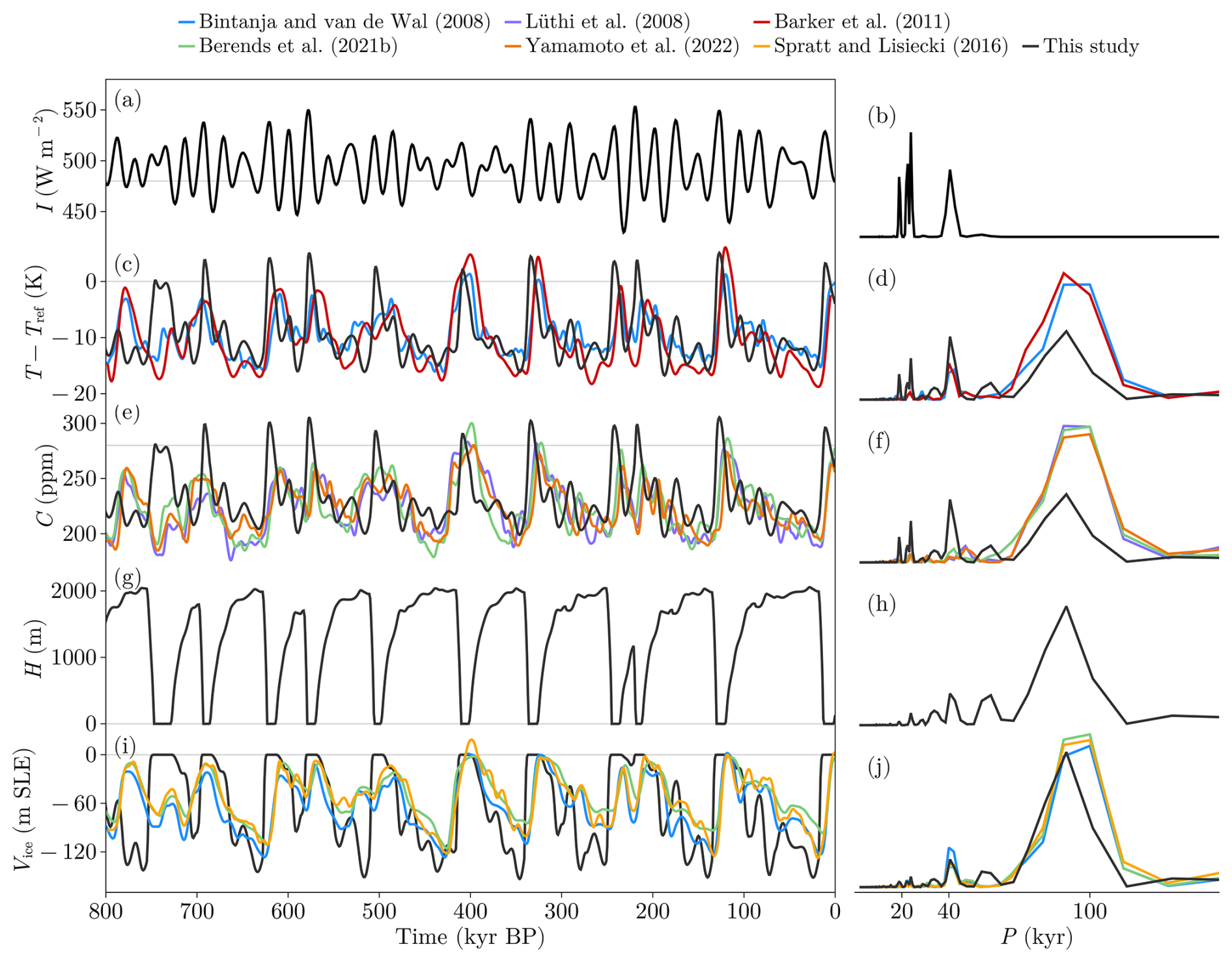
Figure 16 Results of the AGING simulation (black) for τ_α=50 kyr and $C_{\mathrm{s}}=\mathrm{0.3}\times {\mathrm{10}}^{-\mathrm{7}}$ m yr⁻¹ Pa⁻² (in comparison with Bintanja and Van de Wal, 2008; Lüthi et al., 2008; Barker et al., 2011; Spratt and Lisiecki, 2016; Berends et al., 2021b; Yamamoto et al., 2022). Note that the initial conditions are applied at 1000 kyr BP just to let the model equilibrate.

Since PACCO has no spatial dimensions, the ice volume is defined through the product of ice thickness and the potentially glaciated surface S. This can be expressed in meters of sea level equivalent (m SLE) by

$$\begin{array}{}\text{(42)}& V_{\mathrm{ice}}={\displaystyle \frac{{\mathit{\rho }}_{\mathrm{ice}}}{{\mathit{\rho }}_{\mathrm{wtr}}\cdot S_{\mathrm{ocn}}}}\cdot S(T,v_{\mathrm{b}})\cdot H,\end{array}$$

where ρ_wtr is water's density (1000 kg m⁻³); S_ocn (3.625×10⁸ km²) is the oceanic surface of the Earth (Cogley, 2012); and

$$\begin{array}{}\text{(43)}& S=S_{\mathrm{1}}+{\displaystyle \frac{v_{\mathrm{b}}}{\mathit{\nu }}}\cdot \left[\mathit{\pi }\cdot L_{\mathrm{ub}}^{\mathrm{2}}-S_{\mathrm{1}}\right],\end{array}$$

where

$$\begin{array}{}\text{(44)}& S_{\mathrm{1}}={\displaystyle \frac{T_{\mathrm{ref}}-T}{A_{\mathrm{th}}}}\cdot \mathit{\pi }\cdot L^{\mathrm{2}}.\end{array}$$

This equation relies on the fact that a theoretical ice sheet is a symmetrical dome (π⋅L²) whose extension can be modified by anomalies in regional climate $(T-T_{\mathrm{ref}})\cdot A_{\mathrm{thr}}^{-\mathrm{1}}$. However, if the sliding regime is significant, that profile is less parabolic, and thus a correction due to an sliding expansion is taken into account: $v_{\mathrm{b}}\cdot {\mathit{\upsilon }}^{-\mathrm{1}}$. Note that A_thr is the thermal amplitude provided by a certain extent of the ice sheet, and υ is the typical velocity in an ice stream.

Comparison of PACCO's results with proxy data (Fig. 16) shows that for the main variables of the model (T and H), the periodograms exhibit greater power around 100 kyr while maintaining certain power in obliquity and precession bands. This indicates that the nonlinear response of the system is effectively amplified with this new parameterization of albedo. In addition, the comparison of the time series (panels c, e and i from Fig. 16) shows great correlation, indicating that both the amplitude and timing of the GIV are well captured. The evolution of V_ice matches the proxy record qualitatively well despite its simple representation.

In this model configuration, deglaciations start because the first term of Eq. (28) (i.e., the effective shortwave radiation I_eff, Eq. A1) increases ablation thanks to the aging in ice albedo (Fig. A3). At a certain time this contribution is high enough to outweigh snowfall, and the glacial termination starts. This process is enhanced with the ice-sheet surface elevation at the end of the glacial termination. This phenomena can be seen in Fig. 17, where we have represented the trajectories of H as a function of the insolation forcing. This diagram explicitly shows the nonlinearities in the system: ice starts to grow when insolation becomes low enough to allow its persistence over several precession and obliquity cycles, until the effective shortwave I_eff outweighs the accumulation. Then, a glacial termination is triggered.

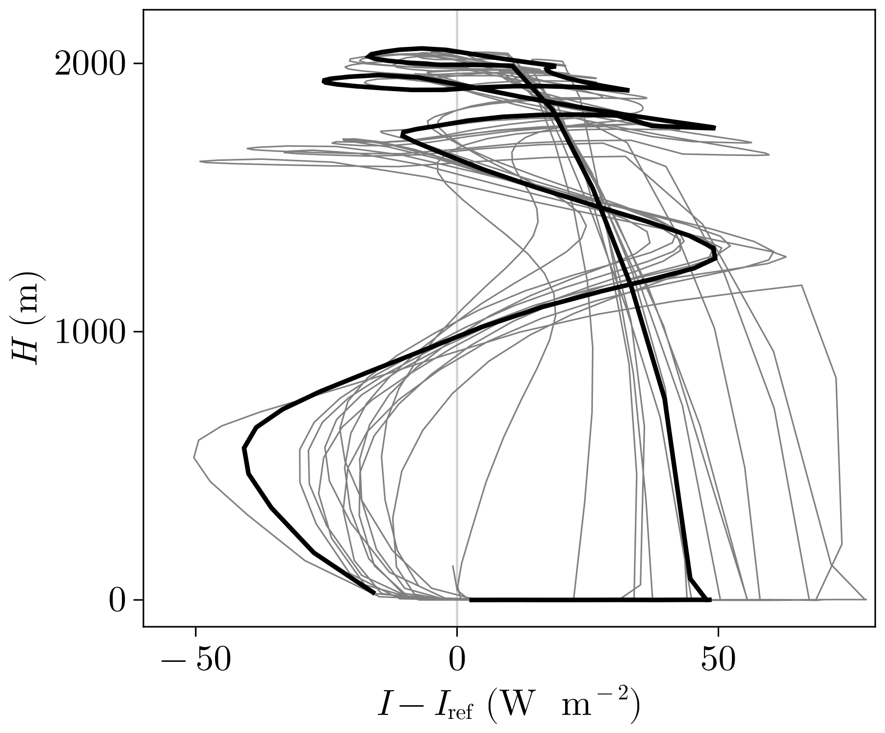
Figure 17 Trajectories of the AGING experiment with τ_α=50 kyr and $C_{\mathrm{s}}=\mathrm{0.3}\times {\mathrm{10}}^{-\mathrm{8}}$ m yr⁻¹ Pa⁻². We highlight the last glacial cycle in black.

3 Discussion

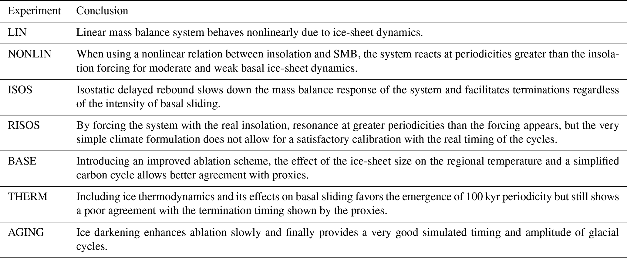
What is the minimum number of required physical processes necessary to satisfactorily simulate glacial–interglacial cycles? This is the question that guides the following discussion. By sequentially increasing the complexity of our simple model, we have evaluated the mechanisms that ultimately facilitate capturing the right timing and amplitude of glacial cycles (see Table 3).

We have seen that the last configuration of PACCO (AGING experiment, Sect. 2.7) produces results that highly correlate with various paleoclimatic records. The mechanisms that trigger GIV in this configuration are in agreement with state-of-the-art hypotheses relying on more comprehensive models (Ganopolski and Calov, 2011; Abe-Ouchi et al., 2013, among others). The 100 kyr periodicity is a result of both ice-sheet dynamics and interactions with the climate. On one hand, ice-sheet velocity determines the responsiveness of the ice sheet to the insolation forcing. The strength of sliding affects the level of ice-sheet sliding and thus facilitates its synchronization with the forcing via ice discharge. Therefore, the periodicity of the system response varies with sliding. On the other hand, isostasy and ice aging provide two feedbacks that amplify the lagged deglaciations. Both processes become more and more important when the ice persists over time. When the albedo is low enough, an increase in insolation can trigger a deglaciation that is reinforced through the melt–elevation feedback. We have also seen that ice-sheet thermodynamics could play an important role in this variability since it increases the ice basal velocity. However, in our case ice aging is more effective, because it introduces a mechanism that persists over multiple glacial cycles.

An advantage of PACCO is that it is not necessary to perform a strict calibration of each model parameter to obtain GIV, which appears to be a robust model feature. It would have been possible to perform thousands of permutations to obtain a better match with proxies. However, this goes beyond the scope of this paper, since our purpose is to build the structure of a physically explicit conceptual model with which to study the dynamics of the climate–ice-sheet interaction.

Finally, the sensitivity of the ice sheet to sliding remains to be explained and attributed. One possible mechanism could be the rigidity of the substratum on which the ice sheet is formed, as proposed by the regolith removal hypothesis (Clark and Pollard, 1998; Ganopolski and Calov, 2011; Willeit et al., 2019; Ganopolski, 2024) in the context of the Mid-Pleistocene Transition. This hypothesis states that a change in the ice sheet's sliding capacity due to the elimination of the weak substratum produced during the Pliocene could have facilitated the long periodicities of the Late Pleistocene GIV. Investigating this mechanism, together with reproducing the GIV of the entire Pleistocene, is reserved for future work.

Table 3 Summary and main conclusions of the experiments performed in this work.

4 Conclusions

Here we have developed a simple physically based model in order to sequentially identify the mechanisms responsible for GIV of the last 800 kyr. Our model is novel in the way it is formulated because the equations related to ice dynamics are obtained through spatial lumping of ice-sheet modeling equations. We have seen that in PACCO features of Late Pleistocene proxy records are reproduced due to both ice-sheet dynamics and interactions with the climate. The delayed isostatic response and the thermodynamical control on basal sliding add a slow component to the system. This process accentuates the modulation of the ice-sheet size via basal dynamics and produces the characteristic asymmetry in the cycles (in agreement with Abe-Ouchi et al., 2013). Moreover, the aging of ice due to its natural darkening (given by compaction and dust deposition) provides an additional mechanism to the ablation rate, which allows for glacial terminations when ice sheets are big enough. This trigger is activated when the insolation reaches a certain threshold at which melting outweighs snowfall. The combined contribution of ice-sheet dynamics, isostatic rebound and ice darkening explain the 100 kyr paradox and allow reproducing the power spectrum of glacial cycles along with good timing for glacial terminations with respect to the paleoclimatic records (in agreement with Ganopolski and Calov, 2011).

All these conclusions are subjected to the simplicity of the model, regarding the accuracy of the results and the performed approximations. However, to our knowledge, PACCO is the first conceptual model to explicitly incorporate the most important processes and to produce the Quaternary glacial–interglacial cycles with minimal physics. It opens a new way of conceptual modeling that allows different hypotheses to coexist and be isolated from one another.

Appendix A: Further analysis of the THERM and AGING experiments

A1 THERM sensitivity to sliding factor C_s

A sensitivity experiment using C_s was performed for the THERM configuration. Figure A1 shows that a value higher than 10⁻⁷ produces asymmetric oscillations since THERM needs highly active dynamics.

A2 AGING sensitivity to sliding factor C_s

A sensitivity experiment with respect to the sliding factor C_s was performed for the AGING configuration (Fig. 14). Figure A2c shows that a value from 10⁻¹⁰ to 10⁻⁷ (Pollard and DeConto, 2012) produces asymmetric oscillations similar to those that would be expected from GIV.

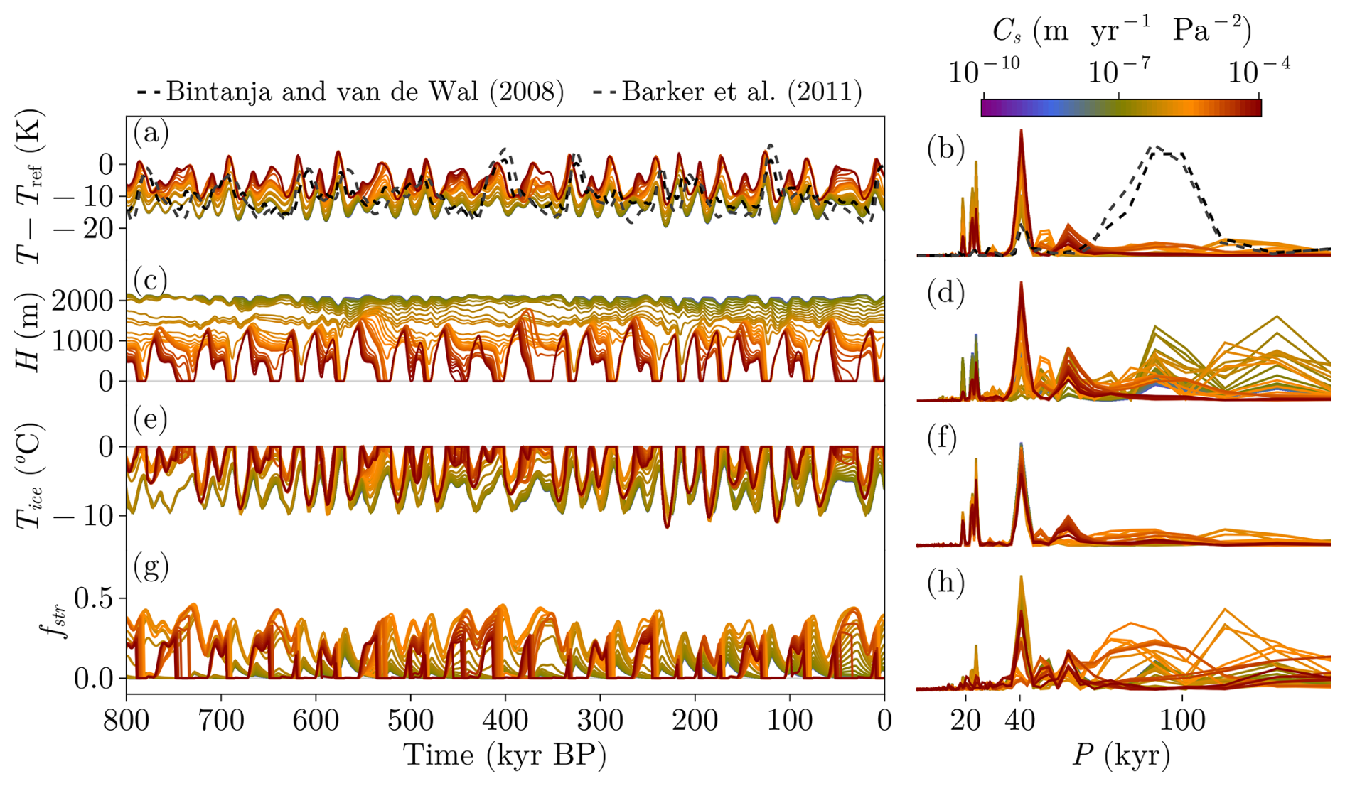
Figure A1 Results of a THERM experiment using different Cs values and τ_kin=10 kyr. (a, c, e) Time series obtained from the model using different sliding factors. (b, d, f) Normalized periodograms obtained from the time series in the left column. Note that when normalizing spectra, series were cut off for periods larger than 200 kyr.

A3 Mechanisms of glacial termination with the AGING configuration

The effective insolation received by ablation is defined from Eq. (28) as

$$\begin{array}{}\text{(A1)}& I_{\mathrm{eff}}=(\mathrm{1}-\mathit{\alpha })\cdot \left(I-I_{\mathrm{ref}}\right),\end{array}$$

which is limited to positive values. I_eff is modulated by albedo aging (Fig. A3b); therefore, the contribution of shortwave radiation to mass balance increases with time. In this way, if the ice persists for enough time, shortwave contribution can outweigh snowfall and thus initiate a glacial termination.

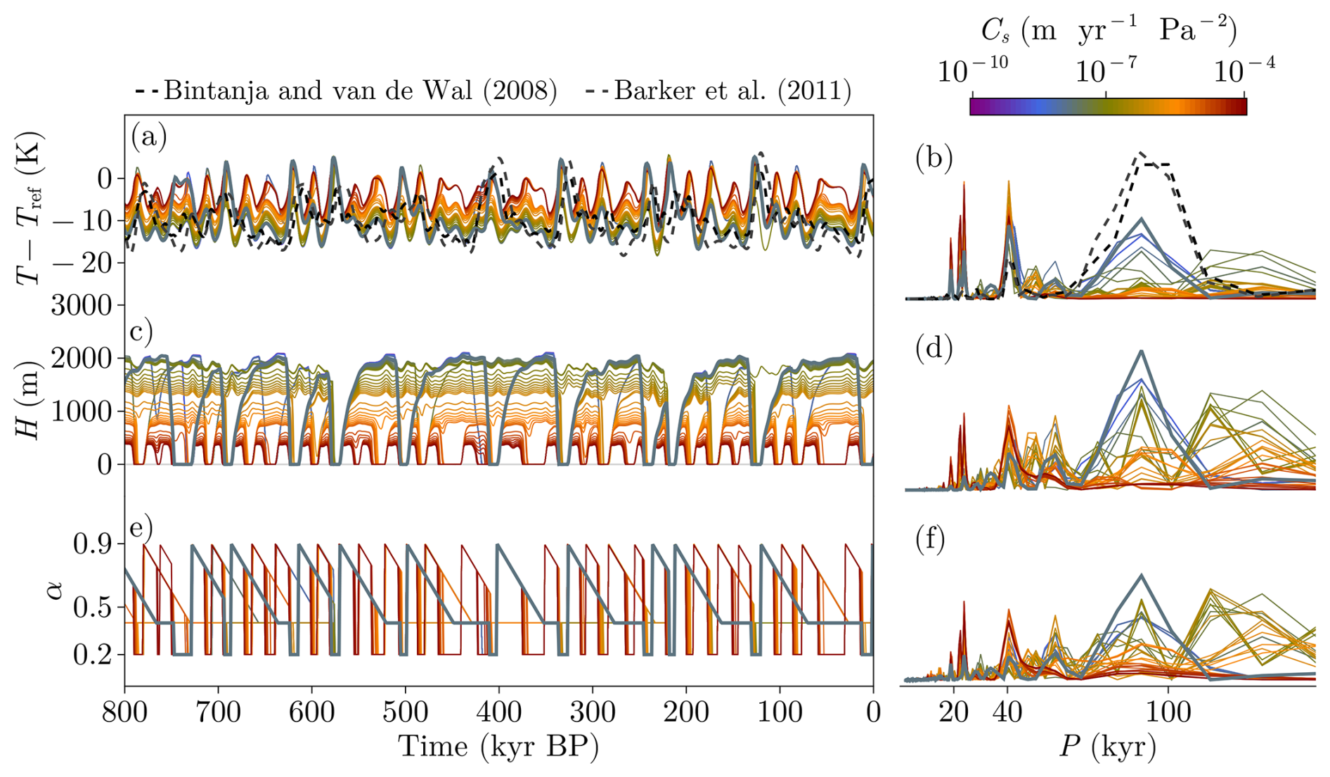
Figure A2 Results of an AGING experiment using different Cs values and τ_α=50 kyr. (a, c, e) Time series obtained from the model using different sliding factors. (b, d, f) Normalized periodograms obtained from the time series in the left column. Note that when normalizing spectra, series were cut off for periods larger than 200 kyr.

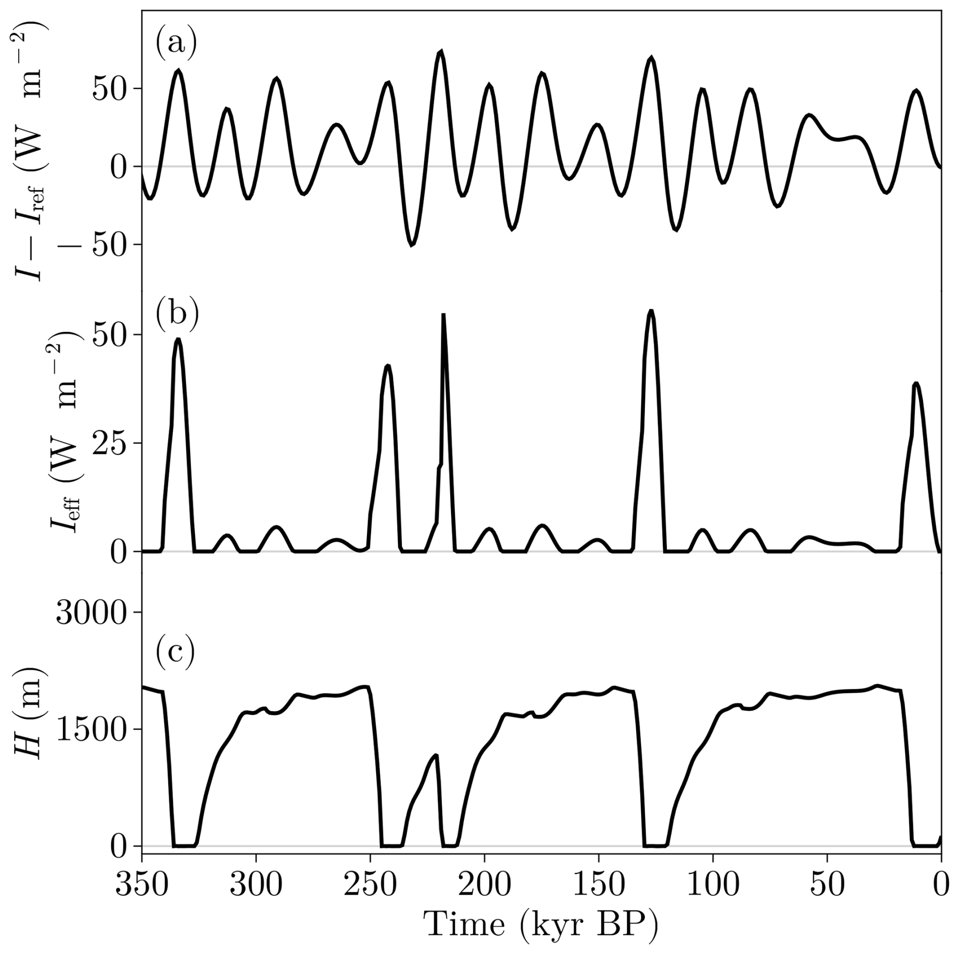
Figure A3 (a) Evolution of insolation relative to I_ref, (b) effective shortwave radiation and (c) ice thickness in the AGING experiment (τ_α=50 kyr, $C_{\mathrm{s}}=\mathrm{0.8}\times {\mathrm{10}}^{-\mathrm{8}}$ m yr⁻¹ Pa⁻²).

Appendix B: Absolute periodograms of experiments performed

Although the absolute value of power spectral density (PSD) of each experiment in this work is not relevant, we provide a summary of every experiment performed without normalizing the distribution in Fig. B1.

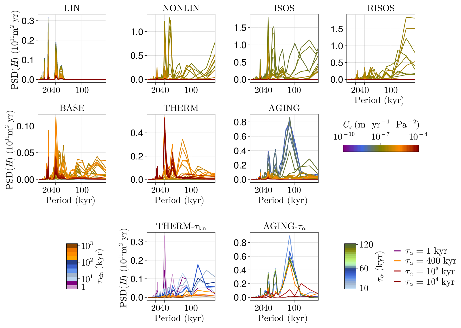
Figure B1 Power spectral density of ice thickness PSD(H) for each experiment performed. Note that the vertical axes are different for each panel and that the colors change according to each experiment.