Estimating ocean heat content from the ocean thermal expansion parameters using satellite data

Ocean heat content (OHC) is a depth-integrated physical oceanographic variable used to precisely measure ocean warming. Because of the limitations associated with in situ conductivity, temperature, and depth (CTD) data as well as ocean reanalysis system products, satellite-based approaches have gained importance in estimating the daily to decadal variability of OHC over the vast oceanic region. Efforts to minimize the biases in satellite-based OHC estimates are needed to realize the actual response of the ocean to the brunt of climate change. In the current study, an attempt has been made to better implement the satellite-based ocean thermal expansion method to estimate OHC at 17 depth extents ranging from the surface to 700 m. To achieve this objective, artificial neural network (ANN) models were developed to derive thermosteric sea level (TSL) from a given dataset of sea surface temperature, sea surface salinity, geographical coordinates, and climatological TSL. The model-derived TSL data were further used to estimate OHC changes based on the thermal expansion efficiency of heat. Statistical analysis showed high correlation coefficients and low errors in the validation of model-derived TSL and OHC for the 700 m modeling depth (N 388 469, R 0.9926 and 0.9922, RMSE 1.16 m and 1.56 GJ m⁻², MBE −0.19 m and −0.24 GJ m⁻², MBPE −0.46 % and −0.03 %, MAE 0.76 m and 1.03 GJ m⁻², and MAPE 2.34 % and 0.13 %) and nearly similar results at the remaining modeling depths. These results suggest that the proposed ANN models are capable of generating satellite-based daily OHC maps by covering both shallower and deeper oceanic regions of varying bathymetry levels (≥20 m). In addition, the first-ever attempt to estimate the ocean thermal expansion component (i.e., TSL) from satellite data was successful, and the model-derived TSL can be used to obtain high-end sea level rise products in the global ocean.

1 Introduction

Owing to the vast spatial coverage and high heat capacity, oceans balance the planet's temperatures by absorbing 89 % of the excess atmospheric heat caused by the greenhouse effect and global warming (Abraham et al., 2013; IPCC, 2014; Roemmich et al., 2015; Riser et al., 2016; Trenberth et al., 2016; Meyssignac et al., 2019; Von Schuckmann et al., 2023). A precise understanding of the depth-wise penetration of this heat and its accumulation in the upper-oceanic layers is of great importance to the scientific community (Liang et al., 2015; Baxter, 2016; IPCC, 2022). Ocean heat content (OHC), a depth-integrated physical oceanographic variable that refers to the amount of heat energy accumulated between any two depths, has gained attention in various studies of the Earth's energy imbalance (Von Schuckmann et al., 2016; Trenberth et al., 2016; Cheng et al., 2017; Meyssignac et al., 2019; Cheng et al., 2022). Thus, accurate estimation of OHC changes at various depth extents is vital and is the motivation of the current study.

To obtain a complete picture of OHC changes at different depths, direct measurements of in situ conductivity, temperature, and depth (CTD) profiles are necessary. These in situ measurements of the ocean properties are limited in terms of depth and spatial coverage, leading to the biased global reconstruction of OHC estimates owing to sparse measurement data and spatial coverage deficiencies (Jagadeesh et al., 2015; Meyssignac et al., 2019; Marti et al., 2022). However, in situ CTD profile measurements have been used to develop and validate different OHC models (Momin et al., 2011; Jagadeesh et al., 2015; Su et al., 2020; Vijay Prakash and Shanmugam, 2022). On the other hand, synthetic CTD profile data generated by ocean reanalysis systems (ORAs) have been used to study OHC variability on spatial and temporal scales (Balmaseda et al., 2015; Palmer et al., 2017). More recently, satellite-based methods have become crucial to overcome the limitations associated with in situ CTD data and ORA products, to ensure the OHC trend at a global scale, and to understand the evolution of the Earth's climate system (Meyssignac et al., 2019; Vijay Prakash and Shanmugam, 2022).

The existing satellite-based OHC algorithms can be broadly grouped into three approaches based on the principles and parameterizations employed: (i) internal tide oceanic tomography (ITOT), (ii) ocean net surface heat fluxes, and (iii) ocean thermal expansion coefficient. Apart from these approaches, research is exploring ways to make use of tidal magnetic satellite observations (Irrgang et al., 2019), electrical conductance (Trossman and Tyler, 2019), and atmospheric oxygen and carbon dioxide concentrations (Resplandy et al., 2018) to infer OHC changes. The ITOT technique involves correlating satellite-altimeter-derived internal tide phase changes with ocean warming to estimate OHC variability. This technique is still at the proof-of-concept level, and associated challenges remain to be addressed (Zhao, 2016, 2017; Meyssignac et al., 2019). OHC estimation through ocean net surface heat fluxes employs several assumptions and approximations in deriving the input parameters to compute radiative and turbulent heat fluxes, which in turn leads to higher uncertainty in global OHC changes (Wild et al., 2015; L'Ecuyer et al., 2015; Meyssignac et al., 2019).

On the other hand, the ocean thermal expansion method is a promising technique for the estimation of OHC by considering the thermosteric sea level (TSL) and expansion efficiency of heat (EEH). Numerous satellite-based OHC models have been developed based on the sea surface height anomaly from altimeters, water mass change equivalent sea level anomaly from the Gravity Recovery and Climate Experiment mission (GRACE), sea surface temperature from the various radiometers on board satellites, and wind speed and stress from scatterometers and numerical weather models. Pioneering works by White and Tai (1995), Chambers et al. (1997), Polito et al. (2000), and Sato et al. (2000) have attempted to implement the ocean thermal expansion method based on a relationship between OHC and satellite-altimeter-based sea surface height anomaly (SSHA). It should be mentioned that regardless of the source, the volume of seawater changes when it is subjected to heating and cooling, and it is eventually reflected in sea surface topography. The SSHA data recorded by satellite altimeters comprise the sea surface topography changes due to tides, atmospheric pressure, salinity (haline), and barotropic flows along with the thermal effects. The SSHA changes due to tides and atmospheric pressure can be corrected, but the effects of salinity and barotropic flows remain unresolved with the OHC estimates produced by White and Tai (1995) and Chambers et al. (1997). Sato et al. (2000) have introduced a haline correction factor as the integral product of the haline contraction coefficient and salinity anomaly from in situ CTD profile data. Owing to the limitations associated with in situ data, the in situ-based haline correction cannot be applied to satellite-altimeter-based SSHA data while correlating with space- and time-varying OHC data. Jayne et al. (2003) have proposed the Alt-GRACE approach to resolve the effect of barotropic flows in sea surface topography by subtracting the satellite-gravimetry-derived water mass change component from SSHA data. Though the Alt-GRACE approach has improved the accuracy of satellite-based OHC estimates compared to White and Tai (1995), Chambers et al. (1997), Polito et al. (2000), and Sato et al. (2000), the issues associated with the haline effects and other approximations on the ocean thermal expansion coefficient and seawater density data have led to significant uncertainties in satellite-based OHC estimates.

With the advancement of artificial intelligence, several researchers have attempted to model OHC by directly relating it to the satellite-based parameters of relevance by using deep-learning regression techniques (Jagadeesh and Ali, 2006; Momin et al., 2011; Chacko et al., 2015; Jagadeesh et al., 2015; Su et al., 2020, 2021; Marti et al., 2022; Lyman and Johnson, 2023). These deep-learning models have oversimplified the OHC problem by neglecting the effects of salinity and barotropic flows. In addition, no previous work has accounted for the space- and time-varying nature of the ocean thermal expansion coefficient and seawater density in OHC computations. The other common drawbacks of existing works are discussed in Sect. 4.3. Consequently, there is a need to develop a satellite-based model to accurately implement the ocean thermal expansion method to estimate OHC by resolving all the issues associated with salinity variation, barotropic flows, ocean thermal expansion, seawater density, and the choice of temperature and its scale.

Given the above background, we have made a major attempt to develop and implement satellite-based ocean thermal expansion models for estimating OHC changes at various depth extents (such as 20, 30, 40, 50, 100, 150, 200, 250, 300, 350, 400, 450, 500, 550, 600, 650, and 700 m). It enables the research community to generate satellite-based OHC maps of varying bathymetry levels (≥20 m) by covering both shallower and deeper oceanic regions. For this, artificial neural network (ANN) models were developed to estimate TSL for the given sea surface temperature (SST), sea surface salinity (SSS), geographical coordinates, and climatological TSL. The model-derived TSL estimates were then used to model OHC changes by accounting for the expansion efficiency of heat. The proposed models are capable of estimating TSL and OHC at multiple depth extents accurately. The robustness of the new models was tested by comparison of model-derived TSL and OHC with in situ data.

2 Data

2.1 In situ data for model development and in situ-based validation

For this study, in situ CTD profile data (collected by Argo floats) were obtained from the World Ocean Database 2018 (WOD) at the NOAA National Centers for Environmental Information data archive for the period of 2005–2020 (Boyer et al., 2018a). WOD18 has been extensively used by the research community for various ocean applications (Levitus et al., 2009; Momin et al., 2011; Levitus et al., 2012; Cheng et al., 2014; Roemmich et al., 2015; Jagadeesh et al., 2015; Su et al., 2020). WOD18 comprises oceanographic data of=n diverse biogeochemical parameters that have been collected by various institutions, agencies, individual researchers, and data recovery initiatives. The quality-controlled CTD profile data (accepted_value flag) of standard depth levels recommended by the International Association of Physical Oceanography in 1936 were considered in this study to compute the TSL_d and OHC_d parameters and to obtain the SST and SSS data. The standard depth levels considered for deriving the TSL and OHC are given as 20, 30, 40, 50, 100, 150, 200, 250, 300, 350, 400, 450, 500, 550, 600, 650, and 700 m. The in situ TSL_d and OHC_d parameters were computed by applying the integration formulae (Eqs. 1 and 2) to the CTD profile data for the depth range from the ocean surface to the respective standard depth (d), and the corresponding SST and SSS values were extracted. Similarly, the climatological parameters such as TSL_clim,d and OHC_clim,d were computed from the monthly climatological temperature and salinity data of 41 vertical levels obtained from the World Ocean Atlas 2018 (WOA) (Boyer et al., 2018b). The theoretical considerations for computing OHC change at a particular depth extent can be found in Vijay Prakash and Shanmugam (2022) (Vijay Prakash and Shanmugam, 2022), and the same considerations were adopted in this study. The Gibbs-SeaWater (GSW) Oceanographic Toolbox of TEOS-10 (IOC et al., 2010) was used to compute the in situ-based OHC and TSL.

$$\begin{array}{}\text{(1)}& {\displaystyle }{\mathrm{OHC}}_d={\int }_{\mathrm{0}}^d\mathit{\rho }{C}_{\mathrm{P}}\mathrm{\Theta }\mathrm{d}z\text{(2)}& {\displaystyle }{\mathrm{TSL}}_d={\int }_{\mathrm{0}}^d\mathit{\alpha }\mathrm{\Theta }\mathrm{d}z\end{array}$$

Here, OHC_d refers to the heat energy accumulated in an oceanic layer of a depth extent ranging from the surface to a stipulated depth (d) and is given in units of joules per unit area (J m⁻²). Similarly, TSL_d (in m) refers to the thermosteric sea level integrated from the surface to a stipulated depth (d). And Θ is the conservative temperature in Kelvin (derived from in situ temperature, absolute salinity, and pressure), ρ is the seawater density in kilograms per cubic meter (kg m⁻³) (derived from the conservative temperature, absolute salinity, and pressure), C_P is the specific heat capacity (3991.87 J kg⁻¹ K⁻¹), and α is the ocean thermal expansion coefficient (K⁻¹; derived from the conservative temperature, absolute salinity, and pressure).

Python programming was used to prepare the individual databases for all the standard depth levels by extracting CTD profile data from the WOD18 and WOA18 NetCDF files with the help of NetCDF4, NumPy, Pandas, and GSW libraries. Each database (in situ OHC, in situ TSL, in situ SST, in situ SSS, climatological OHC, climatological TSL, and WOA18 geographical coordinates) was divided into two datasets, one for the model development spanning 2005–2016 and the other for validating the model spanning 2017–2020, by ensuring a well distribution in spatiotemporal scales over the global open ocean. The spatial distribution of data points used to model TSL₇₀₀ and OHC₇₀₀ is shown in Fig. A1. The in situ CTD profiles of depth coverage shallower than 700 m are also included in this process of deriving the TSL and OHC of remaining depth extents. Indeed, the numbers of CTD profiles and their distribution in global oceans are higher than the CTD profile density of the modeling depth of 700 m.

2.2 Satellite-based validation

For the validation period of 2017–2020, the NOAA Advanced Very High-Resolution Radiometer (AVHRR) Optimum Interpolation Sea Surface Temperature product (OISST v2.1) was used for daily SST data at 0.25° spatial resolution (Huang et al., 2021). Daily SSS data at the same spatial resolution were obtained from the ORAS5 ocean reanalysis system of the European Centre for Medium-Range Weather Forecasts at the CMEMS portal (Product ID: GLOBAL_REANALYSIS_PHY_001_031) (Zuo et al., 2017). The NetCDF4 and NumPy Python libraries were used to read and resample satellite data to the WOA18 grid and to collocate with the corresponding Argo in situ data points. The accuracy of the satellite-based SST and ORA-based SSS was verified by comparing with Argo-measured SST and SSS data (N=244 722). The observed R, RMSE, MBE, and MAE values in SST and SSS validations are 0.99 and 0.99, 0.51 °C and 0.26 PSU, −0.05 °C and −0.006 PSU, and 0.33 °C and 0.12 PSU, respectively. High correlation coefficients and low errors indicate minimal deviation of satellite-based data from the actual (in situ) data and ensure the reliability of satellite data in accurately representing the physical oceanographic conditions.

3 Methodology

3.1 Theoretical formulations

Ocean thermal expansion is the best proxy to model the heat content accumulated in an oceanic layer. Unlike fresh water, seawater expands when it warms and contracts when it cools to temperatures above its freezing point. The volumetric expansion of seawater is non-isotropic in nature due to the differences in the degree of constraint in different directions. In a vertical direction, atmospheric pressure exerts a normal force on the seawater parcel at the surface. The magnitude of this normal and vertical force is less compared to the horizontal forces exerted by physical barriers such as continental boundaries and geographic features on the ocean floor. It allows the ocean thermal expansion of seawater in the vertical direction rather than the horizontal direction, as the seawater is less constrained in the vertical direction compared to the horizontal direction. The amount of change in seawater volume in response to the net warming or cooling depends on the absolute conservative temperature and ocean thermal expansion coefficient (Eq. 2). Following are the GSW functions (Eqs. 3–5) (IOC et al., 2010) involved in the calculation of TSL (Eq. 2) for the given set of measured temperature (T), practical salinity (SP), pressure (P), longitude (x), and latitude (y).

$$\begin{array}{}\text{(3)}& {\displaystyle }\text{Absolute\hspace{0.17em}salinity}\left(\mathrm{SA}\right)=\mathrm{gswSA}\mathit{\_}\mathrm{from}\mathit{\_}\mathrm{SP}\left(\mathrm{SP}Pxy\right)\text{(4)}& {\displaystyle }\mathrm{\Theta }=\mathrm{gswCT}\mathit{\_}\mathrm{from}\mathit{\_}T\left(\mathrm{SATP}\right)\text{(5)}& {\displaystyle }\mathit{\alpha }=\mathrm{gswAlpha}\left(\mathrm{SA}\mathrm{\Theta }P\right)\end{array}$$

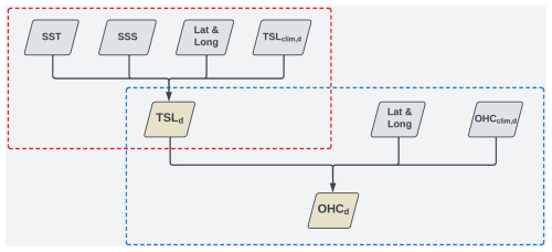
Hence, an attempt has been made in this study to model TSL as a function of SST, SSS, and geographical coordinates. The existing correlations between the proposed input parameters and the targeted output parameter were explored by employing in situ-based data used in the model development process (Fig. 1).

Figure 1 Heat map showing the Pearson correlation coefficients between the input parameters (i.e., SST, SSS, and geographical coordinates) and the output parameter (TSL) of various depth extents.

It is observed that SST has an almost one-to-one correlation with TSL at shallower depth extents and can be solely used to model the thermal expansion of upper-oceanic layers. Despite a decreasing trend in correlation strength when moving towards deeper depths, SST plays a primary role in accounting for TSL variations at deeper depths because of its strong correlations with TSL. Observed weaker correlations between SSS and TSL are plausible owing to salinity's secondary role in TSL variations compared to temperature. However, an increasing trend in correlation coefficients between SSS and TSL is observed towards the deeper depth extents. Hence, SST and SSS are complementary to each other in resolving the TSL variations, and their combination plays a major role in modeling TSL of all depth extents considered in this study. Apart from these physical parameters, absolute salinity used in the computation of seawater density, conservative temperature, and the ocean thermal expansion coefficient is a function of geographical coordinates along with practical salinity and pressure (Eq. 3). By considering all these theoretical considerations and observed correlations, an attempt has been made to model TSL of various depth extents by employing SST, SSS, and geographical coordinates as the input parameters along with the climatological TSL (Fig. 2). Here, TSL_d is an external manifestation of OHC_d stored in an oceanic layer based on EEH_d (Eq. 6). The model-derived TSL is further used to estimate OHC changes (along with climatological OHC as shown in Fig. 2) as follows:

$$\begin{array}{}\text{(6)}& {\mathrm{OHC}}_d={\displaystyle \frac{{\mathrm{TSL}}_d}{{\mathrm{EEH}}_d}},\end{array}$$

where EEH is a conversion factor that explains the relationship between the relative changes in OHC and the corresponding TSL. EEH is not a constant value over the global ocean as it varies as a function of temperature, salinity, and pressure. Hence, ANN modeling is employed in this study to estimate OHC from TSL by accounting for the complex variations in EEH.

Figure 2 Flowchart representing the parameters involved in TSL and OHC modeling. The dashed red and blue boxes represent the TSL and OHC frameworks employed in ANNs, respectively.

3.2 ANN model description

This section explains the various steps and architectures involved in the ANN modeling of TSL and OHC. The multilayer perceptron regressor algorithm of deep neural networks was used to model both TSL and OHC (Pedregosa et al., 2011). It is observed that the input data of geophysical parameters have different units and scales. The range and order of magnitude (O) of SST, SSS, latitude, and longitude data are −1.8 °C to 34.15 °C and O(10¹), 2.53 to 40.45 PSU and O(10¹), −76 to 80° and O(10¹), and −180 to 180° and O(10²), respectively. In addition, the range and order of TSL_clim,d and OHC_clim,d are also distinct and vary with depth extent. Hence, the input data were normalized using the StandardScaler class of scikit-learn and feed-forwarded through the neural networks. This StandardScaler normalizes the raw data to ensure the mean and standard deviation of each input parameter as 0 and 1, respectively. It allows the ANN model to focus on the relative importance and relationships between the input parameters rather than their magnitude. The standardized input data were injected into the corresponding neurons in the input layer and forward-propagated through the hidden layers and then the output layer by applying the random weights and rectified linear unit (ReLU) activation function at each neuron (Fig. 3). The model outputs were compared with the actual data and computed mean squared error (MSE) using a loss function (Eq. 7). In addition, L2 regularization (α_L2) was employed to add a penalty term to the loss value to prevent overfitting. The observed error was then back-propagated through the network to update weights and biases using the Adam optimizer based on the learning rate and gradient of the error (see Eq. 8 in Vijay Prakash and Shanmugam, 2022). This process is repeated until the validation score improves more than 0.0001.

$$\begin{array}{}\text{(7)}& \mathrm{MSE}={\displaystyle \frac{\mathrm{1}}{N}}\sum (Y_{\mathrm{pred},i}-Y_{\mathrm{act},i}{)}^{\mathrm{2}},\end{array}$$

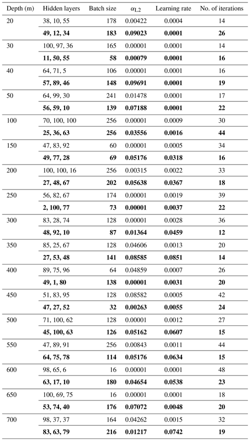
where N is the number of samples, Y_pred,i represents the predicted data, and Y_act,i represents the actual data. The model development work was carried out by employing both the input and output parameters from the in situ sources. It enables the ANN models to implement the input data of any remote sensing sources to produce OHC estimates subject to the reliability and accuracy of those data sources. The particle swarm optimization technique (Kennedy and Eberhart, 1995; Shi and Eberhart, 1998) was employed for hyperparameter tuning, and the hyperparameter combinations corresponding to each modeling depth are presented in Table 1. The Joblib module of the scikit-learn library was used to save all the TSL and OHC models of various depth extents considered in this study, and the same module was used to load the TSL and OHC models of desired depth extent with the help of a unified Python script.

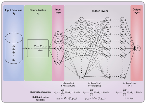
Figure 3 Schematic of the ANN architecture employed in the modeling of TSL and OHC parameters. The flow of the modeling and the associated mathematical transformations and formulations are given by considering a typical ANN architecture with n input parameters, one output parameter, p hidden layers, and q1 to qp neurons in each hidden layer.

Table 1 ANN model hyperparameters employed in TSL (regular font) and OHC (bold font) modeling of various depth extents.

4 Results and discussion

The performance of TSL and OHC models on unseen data from the in situ and satellite sources was assessed using density scattergrams and statistical metrics. These metrics include mean bias error (MBE), mean bias percentage error (MBPE), mean absolute error (MAE), mean absolute percentage error (MAPE), root mean square error (RMSE), Pearson correlation coefficient (R), slope, and intercept (also referred to and presented in Vijay Prakash and Shanmugam, 2022). To better understand the relative magnitude of error metrics, mean values of in situ data were presented for the validation period and used to compute the weighted average of validation metrics across all the modeling depths.

4.1 In situ validations with unseen data

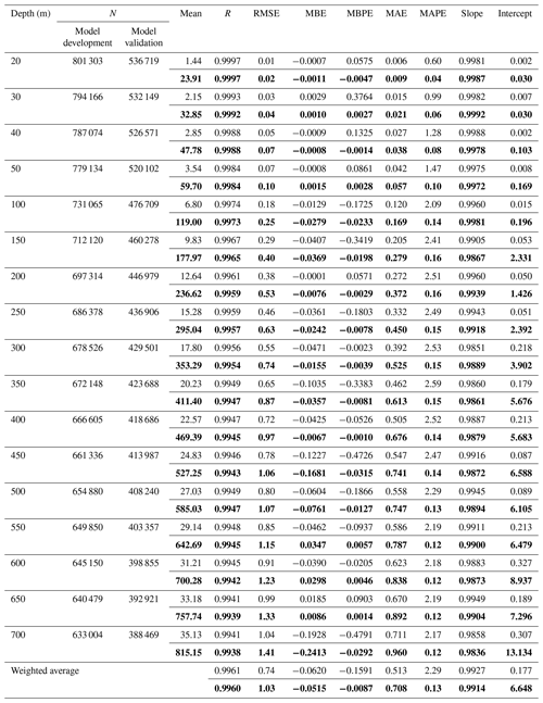
The main objective of the in situ-based validations with unseen data is to evaluate the generalization ability and overall accuracy of TSL and OHC–ANN models on unseen data. For this purpose, the in situ-measured data of SST, SSS, latitude, and longitude were used to predict the model-derived TSL and OHC values, which were then compared with in situ TSL and OHC data. The number of validation data points and their spatial distribution are presented in Table 2 and Fig. A1b. The performance of the TSL models is exceptionally good on unseen data of all the modeling depths without any overfitting (Table 2 and Fig. 4). Similar model performance can also be observed in the case of OHC estimates, as it primarily depends on the TSL estimates (Table 2 and Fig. 5). The high values of R indicate a strong positive correlation between the predicted and in situ OHC (TSL) values. This suggests that the models are generally capable of capturing OHC (TSL) patterns in the data. The slope and intercept of the regression line between predicted and actual values are close to 1 and 0, respectively. This suggests that the model-derived estimates have good agreement with the actual data with a minimal bias. The RMSE values are notably small, implying that the predicted OHC values have a little random error when compared to the actual data. The MBE and MBPE values are close to zero, indicating that the model-derived estimates have a negligible systematic error when compared to the actual values. The low MAE and MAPE values also indicate high accuracy with the model-derived OHC values. These results clearly demonstrate that the proposed ANN models succeeded in generalizing and accurately predicting the OHC (TSL) data with high accuracy.

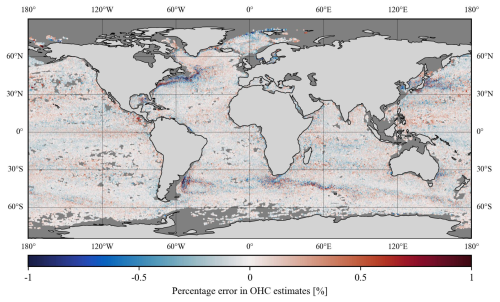
The spatial distribution of the mean percentage error (MPE) over the global open-oceanic regions was computed by averaging the observed percentage errors of all modeling depths available at each pixel (Fig. A2). It is observed that the models' performance is comparatively low over the northwestern parts of the North Atlantic gyre, southwestern parts of the South Atlantic gyre, Kuroshio extension, and Antarctic circumpolar current regions due to the high eddy kinetic energy (Beech et al., 2022; Ni et al., 2023). An elaborate note on the potential sources of the observed MPE values is given in Sect. 4.4. Further, the entire validation dataset was divided into two parts in terms of the observed overestimation and underestimation of data. In the cases of overestimation (underestimation), 95 % of the data points have MPE less than or equal to 0.47 % (0.44 %). The lower values of MPE indicate that the proposed ANN models are capable of capturing OHC patterns in all major oceanic basins and can be used to produce accurate OHC products upon implementation with real-time data.

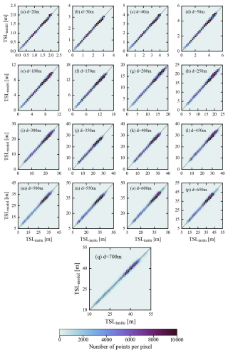
Figure 4 Density scattergrams showing the observed agreement between model-derived TSL values and in situ-measured TSL values during in situ-based validations.

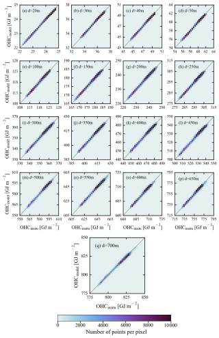
Figure 5 Density scatterplots showing the observed agreement between model-derived OHC values and in situ-measured OHC values during in situ-based validations.

Table 2 Statistical results from the in situ-based validation of TSL (regular font) and OHC (bold font) against in situ data. The units for the various metrics used in TSL and OHC validations are given as follows: mean (m and GJ m⁻²), RMSE (m and GJ m⁻²), MBE (m and GJ m⁻²), MBPE (%), MAE (m and GJ m⁻²), MAPE (%), and intercept (m and GJ m⁻²).

4.2 Satellite-based validations with unseen data

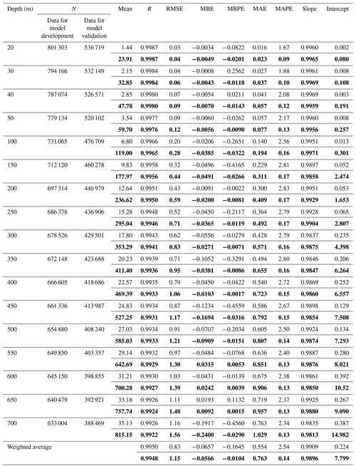
The performance of the proposed ANN models in satellite-based applications has been assessed by injecting daily SST and SSS data from the satellite sources (refer to Sect. 2.2) in place of in situ sources. The choice of satellite sources for SST and SSS data is completely subjective depending on the intended application and their compatibility in terms of spatial and temporal resolutions, whereas geographical coordinate data can be employed from the WOA18 corresponding to the climatological TSL and OHC data. It is recommended to resample SST and SSS data to the WOA18 grid to eliminate the discrepancies arising from the nonuniform spatial references among the input data. The satellite-based SST, ORA-based SSS, latitude, and longitude data were given as the inputs to the ANN models for producing TSL and OHC estimates of all the modeling depths considered in this study. Consequently, the model-derived TSL and OHC estimates were compared with Argo-measured in situ data, and the observed validation results are presented in this section (Table 3 and Figs. 6 and 7).

The performance of the proposed ANN models on satellite-based validation data (Table 3, Figs. 6 and 7) is almost similar to their performance on in situ-based validation data (Table 2, Figs. 4 and 5). However, the models' performance on satellite-based validation data was marginally low compared to the in situ-based validation, likely due to the errors associated with the satellite-based products. According to the statistical results, the R values were observed to be slightly lower by an average percentage decrease of 0.11 % across all the modeling depths. Similarly, the RMSE, MBE, MBPE, MAE, and MAPE values were slightly larger than those observed during the in situ-based validation. This relatively lower performance of the proposed models on the satellite-based validation datasets can also be observed by comparing the spatial maps and the distribution of MPE (Figs. A2 and A3). And 95 % of the data have MPE less than or equal to 0.56 % (0.5 %) in the cases of overestimation (underestimation), which is higher than those reported in Sect. 4.1. Though the performance of the proposed models on satellite-based data is comparatively lower than the in situ-based validation, the observed difference in various validation metrics is insignificant. It indicates the efficiency of the proposed models in estimating OHC from satellite data at various depths over the major oceanic basins. However, it should be noted that the validation results presented in this section may vary with the other sources of satellite-based SST and SSS data.

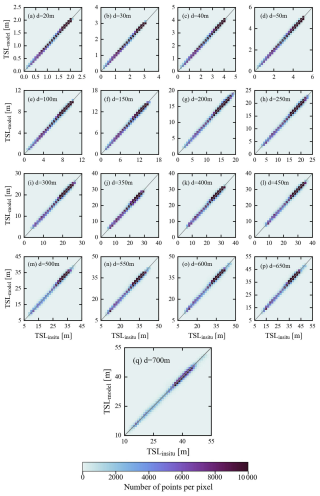
Figure 6 Density scatterplots showing the observed agreement between model-predicted TSL values and in situ-measured TSL values during satellite-based validation.

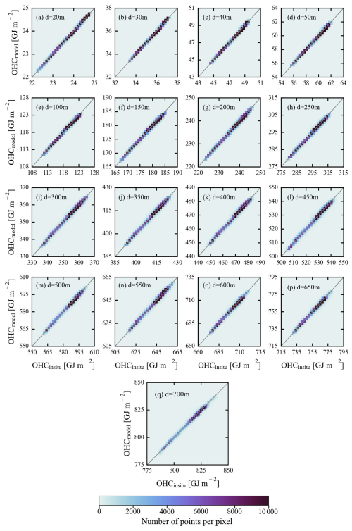
Figure 7 Density scatterplots showing the observed agreement between model-predicted OHC values and in situ-measured OHC values during satellite-based validation.

Table 3 Statistical results from satellite-based validation data of TSL (regular font) and OHC (bold font) against unseen Argo-measured in situ data. The units for the various metrics used in TSL and OHC validations are given as follows: mean (m and GJ m⁻²), RMSE (m and GJ m⁻²), MBE (m and GJ m⁻²), MBPE (%), MAE (m and GJ m⁻²), MAPE (%), and intercept (m and GJ m⁻²).

4.3 Comparison with the contemporary satellite-based OHC models

Comparison of our ANN models with the existing models is crucial to determine the relative uncertainty in the OHC estimates. Previously, an ANN algorithm suite was developed by the National Remote Sensing Centre (NRSC) of ISRO to disseminate the daily OHC products over the northern Indian Ocean (40–120° E, 0–30° N) at a spatial resolution of 0.25° (Ali et al., 2012; Jagadeesh et al., 2015). This algorithm suite includes ANN models to estimate OHC at multiple depth extents such as 50, 100, 150, 200, 300, 500, and 700 m for the given input data of SSHA, SST, and OHC_clim,d. NRSC ANN models estimate OHC changes by employing satellite-altimetry-based SSHA data from the AVISO (Archiving, Validation, and Interpretation of Satellite Oceanographic data) data portal, SST from the Advanced Microwave Scanning Radiometer-2 on board JAXA's Global Change Observation Mission – Water (GCOM-W1), and climatological OHC from the World Ocean Atlas 2009 monthly climatological CTD fields. The multilayer perceptron regressor algorithm of neural networks with three hidden layers was used to estimate OHC of all seven depth extents. The numbers of data points used to develop and validate the NRSC ANN algorithm were 11 472 and 2479, respectively. To compute in situ OHC at different depths, this algorithm employed the Celsius scale, in situ temperature, and average density data instead of the Kelvin scale, conservative temperature, and instantaneous density, respectively (see Eq. 3 in Jagadeesh et al., 2015).

Validation datasets were prepared for the period of 2017–2020 by computing in situ OHC on both Kelvin and Celsius scales for the depth extents of 50, 100, 150, 200, 300, 500, and 700 m from the Argo program. Daily OHC data were downloaded from the NRSC's Bhuvan portal and collocated with the corresponding Celsius-scaled in situ OHC data to evaluate the NRSC ANN models. Similarly, satellite-based SST, ORA-based SSS data, geographical coordinates, and climatological TSL and OHC data were extracted by collocating with Kelvin-scaled in situ OHC data for our ANN models to generate the OHC estimates. Evaluation of these two OHC estimates was done separately by means of the normalized metrics such as R, MBPE, and MAPE (Table 4).

Table 4 Statistical results observed during the validation of model-derived OHC estimates against in situ OHC data.

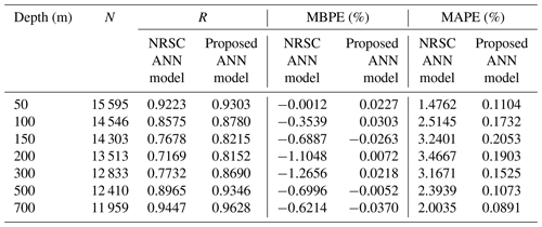
As expected, our ANN models produced relatively highly accurate OHC estimates at all depth extents and hence yielded higher correlation coefficients and lower errors compared to the NRSC ANN models. The accuracy of OHC estimates produced by our ANN model also increased with depth in contrast to that of NRSC ANN OHC estimates. Determination of key input parameters based on a precise theoretical basis, accurate computation of in situ OHC, and use of suitable ANN architectures for each modeling depth enabled our ANN models to produce accurate OHC estimates.

It should be mentioned that SSHA is the combined outcome of temperature (thermosteric), salinity (halosteric), and water mass changes in the oceanic water column. The direct use of satellite-altimeter-derived SSHA without eliminating halosteric and water mass change components results in weaker correlations with OHC. Moreover, different time spans were used in the computation of the mean sea level for AVISO (1993–2012) and monthly climatology data for WOA09 (1955–2006). The combination of merged SSHA data from AVISO/CMEMS and climatological OHC data from WOA18 could lead to discrepancies in OHC estimates. Hence, the prime criterion followed in determining the input parameters in the current study is the theoretical relationship between the input and output parameters rather than the direct usage of all the relevant parameters. The one-to-one relationship between OHC and TSL is employed in the OHC modeling. To arrive at TSL, the theoretical dependency of TSL on temperature, salinity, and geographical coordinates is considered in TSL modeling work. However, SSHA and climatological OHC data for the same base period are desirable and can be used in OHC (TSL) modeling if available in the future.

The Celsius scale can be used to compute in situ OHC where the temperature is always on the positive side. The usage of the Celsius scale when the temperatures are less than zero and greater than the seawater freezing point is not appropriate because of the negative values. In addition, the conservative temperature is an accurate variable to calculate OHC compared to the measured in situ temperature or potential temperature (IOC et al., 2010; Pawlowicz, 2013). Thus, conservative temperatures on the absolute scale (Kelvin scale) are used to compute in situ OHC estimates in the current study. On the other hand, employing instantaneous density rather than an average density value is important to account for the dynamic variations in seawater density.

The vertical distribution of conservative temperature follows a nonlinear profile with a mixed layer at the top, a thermocline in the middle, and a deep ocean layer at the bottom. This suggests that it is appropriate to customize the ANN hyperparameters for each modeling depth. In this study, hyperparameter tuning was performed for each modeling depth and resulted in a better understanding of OHC patterns at various depth extents. Though a clear improvement was achieved with the proposed OHC models, relatively lower correlations were observed for our ANN models in the depth range of 100–300 m over the northern Indian Ocean (refer to Table 4). It indicates that the ANN models generalized the OHC patterns less at the intermediate depths over the northern Indian Ocean, and the corresponding underlying factors are discussed in the following section. Nevertheless, the observed results demonstrated that the proposed ANN models are capable of improving the accuracy and quality of OHC products through the ocean thermal expansion method.

4.4 Potential sources of uncertainty in OHC estimates

The relationship between the surficial parameters (SST and SSS) and depth-integrated parameters (TSL and OHC) is the prime factor determining the efficiency of the proposed OHC models of various depth extents (Klemas and Yan, 2014). This relationship is expected to account for a wide range of geophysical processes including ocean currents, vertical mixing (upwelling and downwelling), stratification, fronts, gyres, eddies, and air–sea interface processes. In addition, different climate modes and oscillations, solar radiation, sea ice, phytoplankton growth, freshwater inputs, and winds can also be considered in this context. Objectively analyzed monthly climatological CTD profiles obtained from WOA18 were used to calculate the monthly climatological mean TSL and OHC over the period of 1955–2017. Hence, these climatological data enabled the ANN models to better generalize the prevailing geophysical processes and subsequent patterns in TSL and OHC of various depth extents. The same can be perceived from the improved accuracy levels observed during the validations carried out on unseen data (refer to Sect. 4.1 and 4.2) and the comparison with NRSC OHC products (Sect. 4.3).

It should be noted that the established relationship between the input parameters (surficial and climatological) and output parameters (TSL and OHC patterns) may not hold in the event of complex geophysical processes where the physical oceanographic conditions differ significantly from the prevailing conditions. Moreover, the relative contributions of these geophysical processes may vary depending on the time and location of the water parcel in oceans. The slightly lower accuracy of the proposed ANN models can be attributed to the influence of these complex geophysical processes. The in situ and satellite-based retrieval of all these atmospheric, surface, and subsurface processes and their incorporation into the ANN models are difficult because of the scarcity or sparsity of the required datasets on different spatial, temporal, and vertical scales. The above factors constitute a potential source of uncertainty in OHC estimates and reduce the generalization ability of the model. Hence, it is advisable to carry out vicarious calibration with the help of contemporary in situ CTD profiles before adopting the OHC estimates for further scientific analyses of specific interest at both regional and global scales. Further efforts are needed to better understand, quantify, and eliminate the different sources of identified uncertainties caused by complex geophysical processes. More in situ CTD profiles are required to be collected and analyzed in such oceanic regions to better account for the associated complex patterns and processes.

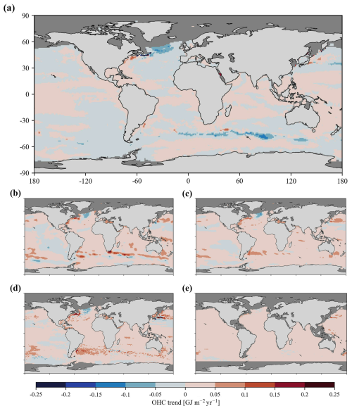
Figure 8 Spatial maps showing the long-term trends of OHC obtained from (a) the current model, (b) NCEI, (c) IAP, (d) PMEL, and (e) OPEN-LSTM products. Note that the oceanic regions shallower than 20 m depth and/or covered with sea ice are masked with a dark gray color.

Figure 9 Time series distribution of global mean OHCA obtained from the current model and the existing OHC products observed over the period 1993–2020. Note that the NCEI time series has been shifted by subtracting 0.3 GJ m⁻² to better compare with the remaining OHC time series plots.

5 Spatiotemporal variability of OHC

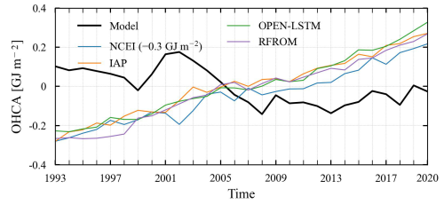
Here, we present the long-term variability of model-derived OHC and its comparison with the existing global OHC products for the period 1993–2020. The time period (1993–2020) was chosen based on the availability of satellite-based input data to generate the model-derived OHC estimates and the existing OHC products considered. Thus, model-derived OHC estimates were generated from 1993 to 2020 at a spatial resolution of 0.25° and computed annual time series of model-derived OHC anomalies (OHCA) with reference to the 1993–2020 long-term mean. It is worth mentioning that the model-derived OHCA estimates presented in this section represent heat changes in both shallower and deep oceanic basins of bathymetry levels ≥20 m. The bathymetry values at each pixel were rounded off to the nearest and lowest modeling depth (d) with the help of GEBCO 2020 bathymetry data, and the corresponding OHCA_d values were considered for each pixel (GEBCO Compilation Group, 2020).

On the other hand, OHCA time series annual maps obtained from various global OHC products disseminated by the National Centers for Environmental Information (NCEI), Institute of Atmospheric Physics (IAP), Pacific Marine Environmental Laboratory (PMEL), and OPEN-LSTM have been employed for comparison. NCEI employs the objective analysis method for in situ CTD profile data from the World Ocean Database 2009 and estimates annual OHCA at a spatial resolution of 1° with reference to the 1955–2006 long-term mean (Levitus et al., 2012). Similarly, IAP employs ensemble optimal interpolation with a dynamic ensemble approach for in situ CTD profile data from the World Ocean Database 2013 and distributes monthly OHC estimates at a spatial resolution of 1° (Cheng et al., 2017). Annual OHC means were computed from IAP monthly OHC data, and annual OHCA estimates were generated with reference to the 1993–2020 long-term mean. Recently, PMEL has developed a random forest regression model to predict OHCA of 0–40, 40–90, 90–190, 190–290, 290–450, 450–700, 700–950, and 950–1450 m depth layers with reference to the 1993–2022 long-term mean. This PMEL random forest regression model employs satellite-based SST, SSHA, latitude, longitude, and time data to predict weekly OHCA estimates at a spatial resolution of 0.25° (Lyman and Johnson, 2023). In the current study, PMEL layer-wise OHCA estimates from surface to 700 m have been summed up at each pixel to arrive at weekly OHCA spatial maps and subsequently computed corresponding annual OHCA estimates. Similarly, Su et al. (2021) have developed a long short-term memory neural network model to produce monthly OHC estimates (OPEN-LSTM) at a spatial resolution of 1°. OPEN-LSTM employs satellite-based SSHA, SST, and zonal and meridional components of sea surface wind, latitude, longitude, and day of the year to predict monthly OHC. Annual OHC means were computed from OPEN-LSTM monthly OHC data, and annual OHCA estimates were generated with reference to the 1993–2020 long-term mean.

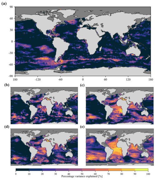
Our model-derived annual OHCA estimates were regridded to 1° spatial resolution to maintain uniform spatial reference among all the OHC products considered. As the proposed models are built for open-oceanic regions, the regions covered by sea ice are masked in both the North and South Pole by verifying the corresponding sea ice concentration data obtained from the National Snow and Ice Data Center (Meier et al., 2021). Subsequently, long-term variability maps (Fig. 8) and time series plots (Fig. 9) were produced to compare model-derived OHC estimates with the existing global OHC products. Further, the information on percentage variance explained (PVE) by the observed long-term trend values is provided to realize the short-term trends or periodic signals in OHC variability (Fig. A4). Higher PVE values indicate a persistent increase or decrease in OHC throughout the study period, and vice versa.

Lower magnitudes of long-term warming and cooling trends (±0.05 GJ m⁻² yr⁻¹) are observed in most of the global ocean (Fig. 8a). The corresponding PVE values are observed to be very low (≤30 %), which indicates intermittent trends in the majority of the global ocean rather than persistent warming or cooling (Fig. A4a). The same can be observed from the nonlinear distribution of model-derived OHCA time series, indicating short-term periods of alternate warming and cooling during the study period (Fig. 9). However, the oceanic regions linked to the Kuroshio current, Gulf Stream, Antarctic circumpolar current, North Atlantic cold blob, and southeastern Pacific are experiencing relatively higher magnitudes of persistent warming or cooling (±0.1 to 0.15 GJ m⁻² yr⁻¹, PVE 50 %–90 %).

The spatial patterns of OHC trends observed from NCEI (Fig. 8b), IAP (Fig. 8c), and PMEL (Fig. 8d) products are almost similar and show relatively more warming regions compared to the model-derived OHC estimates (Fig. 8a). NCEI, IAP, and PMEL products indicate persistent warming conditions over the vast oceanic regions of the Pacific, Atlantic, and Indian Ocean, with higher PVE values (Fig. A4b–d). The same can be observed from the persistent long-term warming throughout the study period (Fig. 9). On the other hand, OPEN-LSTM OHC estimates indicate lower warming patterns all over the globe except the North Atlantic cold blob and some parts of the Antarctic circumpolar current (Fig. 8e), with higher PVE values over vast oceanic regions of the Pacific, Atlantic, and Indian Ocean (Fig. A4e). As a result, OPEN-LSTM also showed persistent long-term warming throughout the study period (Fig. 9).

The observed time series plots indicate contrasting trends between the current OHC model and the existing products. The time series plot of model-derived OHCA indicates alternate periods of short-term cooling and warming during the study period. Global open oceans witnessed a cooling trend of −0.017 GJ m⁻² yr⁻¹ (PVE 76.99 %) during 1993–1999, a warming trend of +0.069 GJ m⁻² yr⁻¹ (PVE 92.73 %) during 2000–2002, a cooling trend of −0.054 GJ m⁻² yr⁻¹ (PVE 99.71 %) during 2003–2008, and a warming trend of +0.007 GJ m⁻² yr⁻¹ (PVE 36.50 %) during 2009–2020. The observed results indicate the efficiency of the current model in capturing the ocean cooling during 2003–2006 (Loehle, 2009; Lyman et al., 2006) and the global warming hiatus during 1998–2013 (Trenberth, 2015), whereas the observed time series plots of NCEI, IAP, PMEL, and OPEN-LSTM products indicated persistent warming trends of +0.017 GJ m⁻² yr⁻¹ (PVE 95.75 %), +0.019 GJ m⁻² yr⁻¹ (PVE 97.94 %), +0.0198 GJ m⁻² yr⁻¹ (PVE 97.19 %), and +0.0195 GJ m⁻² yr⁻¹ (PVE 97.48 %), respectively. However, full-depth pan-global OHCA estimates by including OHC estimates over ice-covered oceanic regions are required to substantiate these global ocean cooling and global warming hiatus signatures and to realize the role of excess heat added by anthropogenic climate change.

6 Conclusions

Accurate reconstruction of OHC and analysis of its regional patterns and long-term global records are critical for estimating the Earth's energy imbalance and understanding the evolution of climate change. Owing to the lack of instrumentation to cover geographic and depth ranges, OHC estimates from in situ-measured temperatures are temporally limited and insufficiently widespread to capture spatiotemporal changes and structures. OHC estimates from either different mapping methods or ocean reanalyses (ORAs) have yielded large uncertainties in past studies. Thus, improving OHC estimates through a novel satellite-based method is a major step forward in overcoming sparse observations and reducing the uncertainty in OHC trends. In this study, we proposed an artificial network model to estimate OHC changes in global open oceans. The proposed ANN model incorporates the ocean thermal expansion method as a promising tool to estimate OHC changes from satellite data. Accurate implementation of the ocean thermal expansion method was challenging due to the inability of the present-day satellite systems to directly measure the ocean thermal expansion–contraction component. In this study, we proposed a satellite-based novel approach to better implement the ocean thermal expansion method by establishing a relationship between surficial parameters such as SST and SSS and subsurface T–S profiles. This model predicts the depth-integrated TSL component by making use of SST and SSS data and then utilizes the predicted TSL to estimate OHC changes. For this application, we developed ANN models for TSL and OHC of various depth extents such as 20, 30, 40, 50, 100, 150, 200, 250, 300, 350, 400, 450, 500, 550, 600, 650, and 700 m. The performance of these TSL and OHC models was assessed by carrying out in situ-based and satellite-based validations using unseen in situ CTD profiles from the Argo program. Observed high correlations and low errors indicated that the proposed ANN models performed exceptionally good on unseen data of all modeling depths without any overfitting and can be used in conjunction with sea ice thermodynamics-based OHC models of the ice-covered oceans (Vijay Prakash and Shanmugam, 2022) to better study pan-global OHC changes by covering both open and ice-covered oceanic regions of varying bathymetry levels (≥20 m).

The model development and validation databases were prepared by using in situ CTD profiles obtained from the Argo program and collocated with the corresponding satellite-based daily data of SST (AVHRR v2.1) and SSS (ORAS5). The multilayer perceptron regressor algorithm of deep neural networks was used and its architecture was optimized by evaluating different combinations of hyperparameters for each modeling depth using the particle swarm optimization technique. Precise consideration of theoretical aspects in the selection of input parameters, accurate computation of in situ OHC, and customized ANN architectures enabled the proposed models to establish accurate relationships between the surficial parameters and depth-integrated OHC (TSL) of various depths extents. The overall performance of the proposed models on satellite data was good, suggesting that these models can be used for a variety of applications subject to accuracy requirements and can produce more accurate satellite-based OHC (TSL) estimates at various depth extents than previously possible. However, the influence of complex geophysical processes on the generalization ability of ANN models is discussed, and the proposed models generalized the data relatively less in the event of complex geophysical processes. Further research should focus on the implementation of these models over oceanic regions with complex geophysical processes. More in situ CTD profiles need to be collected and analyzed in such oceanic regions to better account for the associated complex patterns. However, the scope of the current research includes minimizing the observed marginal gap by exploring new methods and parameterizations in satellite-based OHC modeling.

Appendix A

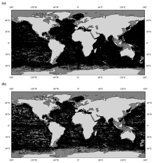
Figure A1 The spatial distribution of in situ data points used for (a) model development (N=633 004 Argo CTD profiles) and (b) validation (N=388 469 unseen Argo CTD profiles) in the case of TSL₇₀₀ and OHC₇₀₀.

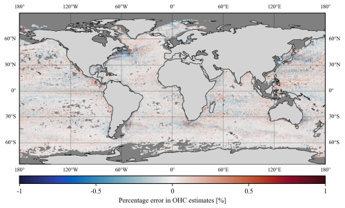
Figure A2 Spatial distribution of mean percentage errors observed during the in situ-based validation of OHC models. The oceanic regions shallower than 20 m and/or covered with sea ice are marked with a dark gray color.

Figure A3 Spatial distribution of mean percentage errors observed during the satellite-based validation of OHC models. The oceanic regions shallower than 20 m and/or covered with sea ice are marked with a dark gray color.

Figure A4 Spatial maps showing the percentage variance explained by the OHC trends obtained from (a) the current model, (b) NCEI, (c) IAP, (d) PMEL, and (d) OPEN-LSTM products. Note that the oceanic regions shallower than 20 m depth and/or covered with sea ice are masked with a dark gray color.