Paleogeographic numerical modeling of marginal seas for the Holocene – an exemplary study of the Baltic Sea

The sustainable management of marginal seas is based on a thorough understanding of their evolutionary trends in the past. The paleogeographic evolution of marginal seas is controlled not only by global and regional driving forces (eustatic sea-level change and isostatic/tectonic movements) but also by sediment erosion, transport, and deposition at smaller scales. Consistent paleogeographic reconstructions at a marginal sea scale considering the global, regional, and local processes are yet to be derived, and this study presents an effort towards this goal. We present a high-resolution (0.01°×0.01°) paleogeographic reconstruction of the entire Baltic Sea and its coast for the Holocene period by combining eustatic sea-level change, glacio-isostatic movement, and sediment deposition. Our results are validated by comparison with field-based reconstructions of relative sea level (RSL) and successfully reproduce the connection/disconnection between the Baltic Sea and the North Sea during the transitions between lake and sea phases. A consistent map of Holocene sediment thickness (SED) in the Baltic Sea has been generated, which shows that relatively thick Holocene sediment deposits (up to 36 m) are located in the southern and central parts of the Baltic Sea, corresponding to depressions of sub-basins, including the Arkona Basin, the Bornholm Basin, and the Eastern and Western Gotland Basin. In addition, some shallower coastal areas in the southern Baltic Sea also host locally confined deposits with thicknesses larger than 20 m and are mostly associated with alongshore sediment transport and the formation of barrier islands and spits. In contrast to the southern Baltic Sea, the Holocene sediment thickness in the northern Baltic Sea is relatively thin and mostly less than 6 m. The morphological evolution of the Baltic Sea and its coastline is featured by two distinct patterns. In the northeastern part, the change in the coastline and offshore morphology is dominated by regression caused by post-glacial rebound that outpaces the eustatic sea-level rise, and the influence of sediment transport is very minor, whereas a transgression, together with active sediment erosion, transport, and deposition, has constantly shaped the coastline and the offshore morphology in the southeastern part, leading to the formation of a wide variety of coastal landscapes such as barrier islands, spits, and lagoons.

1 Introduction

The majority of the Earth's coasts and shelf seas are experiencing dramatic morphological changes as a result of the joint effects of natural processes and anthropogenic activities (Mentaschi et al., 2018). Coasts of marginal seas composed of erodible soft material (sands, mud, and moraine) are most variable in this context (Harff et al., 2017; Luijendijk et al., 2018; Hulskamp et al., 2023). At short timescales, their morphology is constantly reshaped by atmospheric and oceanic forcing such as winds, tides and waves, and human interventions (Zhang et al., 2011a; Mentaschi et al., 2018; Weisse et al., 2021). At longer timescales, climate-change-induced oscillations of sea level, ice cover/retreat, isostatic/tectonic movements, and variations in sediment supply from both coastal erosion and riverine transport exert a major control on the morphological development of marginal seas (Zhang and Arlinghaus, 2022). In the forthcoming centuries, relative sea-level rise will increasingly influence coastal morphological change and challenge the defense of coastlines. The sustainable management of marginal seas therefore requires a thorough understanding of the past and future morphological trends of evolution (Hulskamp et al., 2023). Management strategies need to consider the “geo-environmental” change in the past and future to separate natural and anthropogenic driving forces (Neumann et al., 2015) and understand their interplay. Learning from paleo-geomorphological history, particularly the post-glacial period, will help us to understand coastal change in the future (Harff et al., 2017).

The paleogeographic evolution of marginal seas is strongly associated with global and regional driving forces. Climatically controlled eustatic changes (Gale et al., 2002; Berra et al., 2010) interplay with regional settings such as tectonics (Watts, 1982; Vött, 2007) and isostasy (Peltier, 1999, 2007; Lambeck et al., 2010, Spada et al., 2012) and even with local factors such as sediment availability and dynamics (Einsele, 1996). The combination of these overlapping forces influences the relative sea level and may lead to significantly different coastal behaviors in various sections of marginal seas due to spatial heterogeneity of the described force intensity (Rosentau et al., 2021).

Most paleogeographic reconstructions of marginal seas are based on a reversal of relative sea level composed of eustatic sea-level change plus tectonic and glacio-isostatic crustal effects (Uehara et al., 2006; Harff et al., 2007; Yao et al., 2009; Sturt et al., 2013). A few studies have additionally incorporated sediment relocations based on interpolation techniques and information from dated sediment cores but are limited to local areas (Zhang et al., 2014; Xiong et al., 2020; Karle et al., 2021). This study presents a high-resolution numerical paleogeographic reconstruction of the entire Baltic Sea and its coasts for the Holocene period as a set of paleo-digital elevation models by taking into account not only eustatic sea-level change and glacio-isostatic movement but also sediment deposition. As such, this work represents a further step for the comprehensive paleogeographic reconstruction of marginal seas resolving spatial heterogeneity of driving forces across multi-scales. Our motivation is 2-fold: firstly to depict the morphological evolution of a complex marginal sea system in response to the impact of climate change and oceanic sedimentation; secondly to provide a sediment budget analysis of the marginal sea for the Holocene period and to compare this with present-day sediment fluxes from the land to the sea to disentangle natural and anthropogenic impacts.

2 Geological setting

The Baltic Sea is a semi-enclosed intra-continental marginal sea, connected with the North Sea through the Danish Straits (Rosentau et al., 2017). In terms of regional tectonics, the Baltic Sea basin bridges between the East European Craton (EEC), consisting of the Fennoscandian/Baltic Shield (BS) in the northeast, the Russian East European Platform (EEP) in the southeast, and the Central European Basin System in the southwest (Maystrenko et al., 2008). The East and West European Platform are separated by the deep NW–SE-striking tectonic fault system of the Tornquist–Teisseyre Zone (TTZ) and its northwestern prolongation, the Sorgenfrei–Tornquist Zone (STZ) (Uścinowicz, 2014). Northeast of this zone, Precambrian crystalline rocks of the Baltic Shield and undeformed Phanerozoic sediments of the Russian EEP on Precambrian basement form the coastal frame of the Baltic Sea. West of the TTZ, the central Caledonides and Variscides together form the deep sedimentary basin of the Central European Depression filled mainly with Paleozoic and Mesozoic deposits on a basement at a depth of up to 10–15 km (Uścinowicz, 2014). The lowlands are mainly covered by Pleistocene sediments consisting of glacial, glacio-fluviatile, and lacustrine deposits. The Holocene sediment is represented by coastal, lacustrine, and brackish marine deposits (Rosentau et al., 2017). Glaciers have shaped the surface of the mainland surrounding the Baltic Sea and the Baltic Sea basin itself (with an average water depth of 55 m), where they formed a series of sub-basins separated by shallower sills (Hall and van Böckel, 2020). The Danish Straits connect the Baltic Sea with the North Sea through the Kattegat. The humid climate and a positive water balance promote an estuarine circulation and a stratified water body with remarkable vertical and horizontal differences in salinity, density, and temperature in the present-day Baltic Sea (Matthäus and Franck, 1992; Wulff et al., 1990).

The advance and retreat of glaciers during the Quaternary glacial cycles have caused a change in the isostatic loading and unloading of the Baltic Sea basin's crust, leading to a cyclicity in vertical crustal movement correlated to the climate cycles. The relationship between the vertical crustal movement and the sea-level change determines the hydrographic communication between the open North Sea and the Baltic Sea basin. The parts connecting the Baltic Sea basin and the North Sea thus serve the function of a “gate” that is opened or closed by eustacy–isostasy–ice interaction. Correspondingly, the paleogeographic history of the Baltic Sea basin during the Quaternary was ruled mainly by the glacial cycles following the Milankovitch cyclicity. However, because of the erosional effects of the advancing ice sheet, sediments reflecting the geological history by proxy data remained scarce from the pre-glacial period. Andrén et al. (2011) depicted this postglacial history based on the interpretation of proxy data, including basin sediments and markers of paleo-coastlines, by a set of paleogeographic maps (Fig. 1), which are used in our study for qualitative assessment of the results achieved by numerical modeling.

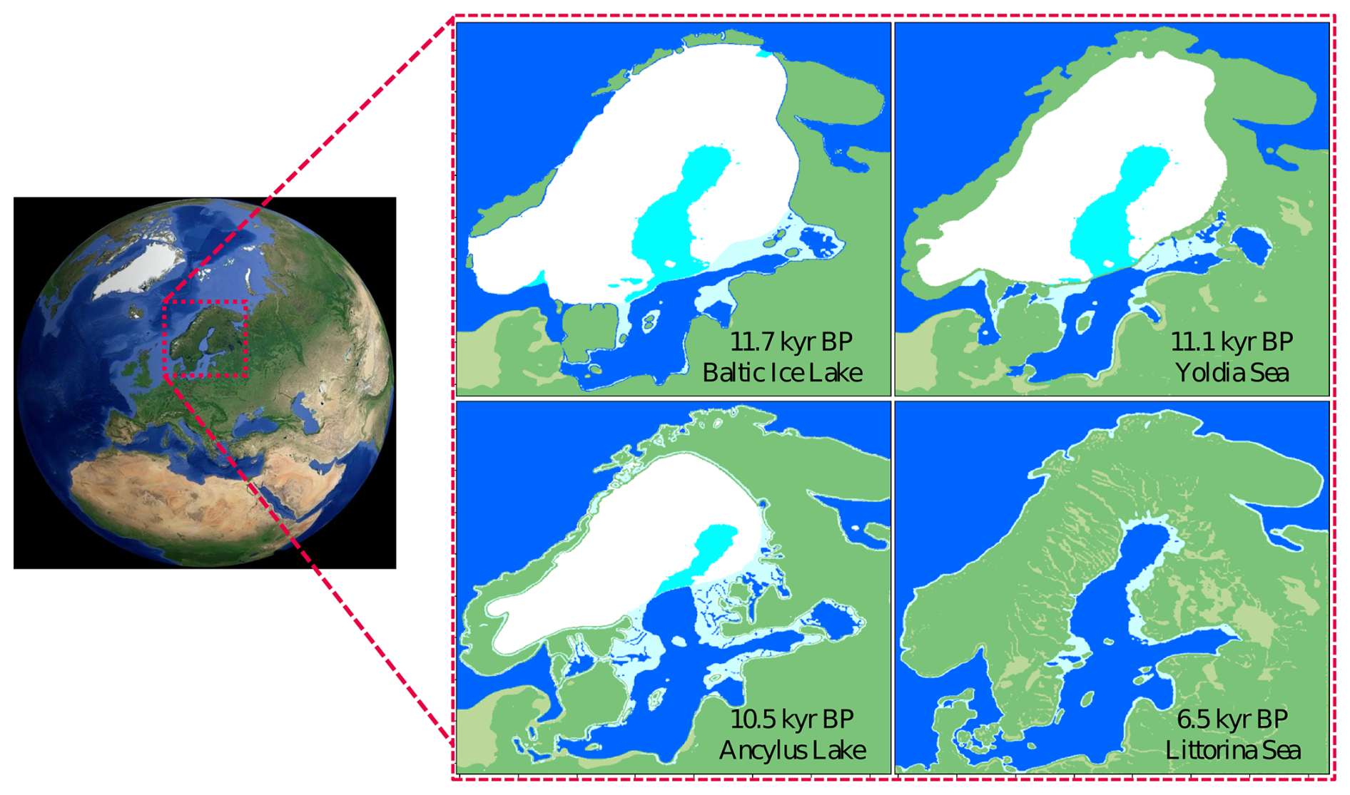
Figure 1 Location of the Baltic Sea (©Google Earth Pro) and paleogeographic maps (modified after Andrén et al., 2011) representing different Holocene stages of the Baltic Sea, including the Baltic Ice Lake/Yoldia Sea transition at 11.7 kyr BP, the Yoldia Sea (end of the brackish phase) at 11.1 kyr BP, the Ancylus Lake (maximum transgression) at 10.5 kyr BP, and the Littorina Sea (most saline phase) at 6.5 kyr BP. Ice cover is shown by the mask in white, blue stands for water, cyan corresponds to present-day water, green marks the present-day land, and olive marks the land in the past.

The evolution of the Baltic Sea since the Last Glacial Maximum (LGM) is characterized by shifts between freshwater and marine sedimentary environments (Andrén et al., 2011). Starting from 16 kyr BP, the Baltic Ice Lake (BIL) was formed in front of the retreating ice sheet filled with glacial meltwater. Initially the water level in the lake was similar to the global sea level, and the meltwater discharged to the Baltic Sea basin flowed through the straits into the North Sea. The connection was, however, ceased due to glacio-isostatic uplift of the straits area at around 14 kyr BP (Björck, 2008). Another reconnection occurred at ∼13 kyr BP via the Central Swedish lowland as a result of the rising water level caused by meltwater discharge to the BIL, but it was interrupted by a short cooling phase of the Younger Dryas at ca. 12.8 kyr BP that caused glacial re-advance (Björck, 1995). As the influence of the isostatic uplift of the Baltic Shield prevailed, the Baltic Sea basin remained disconnected from the North Sea (Fig. 1) until the late stage of the BIL. Glacier retreat and global sea-level rise re-opened the gate connecting the Baltic Sea basin and the North Sea via the Central Swedish lowland (Fig. 1), initiating the brackish Yoldia Sea stage at ∼11.7 kyr BP (Heinsalu and Veski, 2007). At ∼10.7 kyr BP, isostatic uplift again re-closed the gate of the Swedish Depression (Fig. 1) and the Baltic Sea basin turned to a freshwater (lake) environment again (Sohlenius et al., 2001). The initial Ancylus Lake stage was characterized by a rising water level because of meltwater discharge from the ice sheet until reaching a peak at ∼10.5 kyr BP. Afterwards, a decrease in the water level occurred because of a drainage to the North Sea (Lemke et al., 2001; Rosentau et al., 2013). The climate-controlled Holocene sea-level rise in connection with the deforming lithospheric bulge surrounding the Baltic Shield re-opened the gate at the straits, leading to the Littorina transgression starting at ∼8.0 kyr BP (Fig. 1). Since then, the water level in the Baltic Sea has been aligned with the sea level in the open North Sea until the present day.

3 Data and methods

The main target of this study is the generation of a set of paleo-digital elevation models (paleo-DEMs) corresponding to a high-spatiotemporal-resolution (0.01°×0.01° and 500-year interval) reconstruction of the Baltic Sea evolution during the Holocene. Such reconstruction plays a critical role for the purpose of basin analysis (Allen and Allen, 2008), visualization of the past states of marginal seas (Xiong et al., 2020), morphogenetic interpretation (Miluch et al., 2021, 2022), and hydro-morphodynamic modeling of circulation and sediment transport systems (Zhang et al., 2020). Since our reconstruction covers only a relatively short geological time span, i.e., from the initial stage of the Holocene (11.7 kyr BP) until the present day, the key influencing factors considered include eustatic sea-level change, isostatic vertical crust movements, and sediment deposition. Other factors such as sediment compaction play a secondary role at such a timescale (Schmedemann et al., 2008) and therefore are neglected here. An equation following Harff et al. (2017) was applied to generate the paleo-DEMs for any specific time t during the Holocene with reference to the present day (t=0):

$$\begin{array}{}\text{(1)}& {\text{DEM}}_{\mathrm{t}}={\text{DEM}}_{\mathrm{0}}-\mathrm{\Delta }\text{RSL}+\mathrm{\Delta }\text{SED},\end{array}$$

where DEM_t is the paleo-digital elevation model at time t, DEM₀ is the present-day DEM, ΔRSL is the relative sea-level change, and ΔSED is the change in sediment thickness by deposition. The integration of sediment thickness marks the major difference between our reconstruction and existing reconstructions.

The relative sea-level change ΔRSL is calculated by

$$\begin{array}{}\text{(2)}& \mathrm{\Delta }\text{RSL}=\mathrm{\Delta }\text{EC}+\mathrm{\Delta }\text{GIA},\end{array}$$

where ΔEC is the eustatic sea-level change and ΔGIA refers to the glacial isostatic adjustment at time t with reference to present-day conditions.

After successful application of the equations in the South China Sea by Yao et al. (2009) and Xiong et al. (2020), we apply them for the first time to the Baltic Sea basin considering not only GIA and sediment accumulation but also differences in the eustatic sea level and the water level in a regional basin temporarily following a separate regional hydrographic regime when it is disconnected from the open sea.

During brackish marine stages, the sea level of the Baltic Sea basin follows that of the North Atlantic. EC in these stages thus reflects the global (eustatic) sea level. During lake stages, EC reflects the level of the freshwater lake that is fed by precipitation, meltwater from ice, and rivers. In this case, EC on the coast of Fennoscandia influenced by the open ocean is modeled separately from that in the Baltic Sea basin.

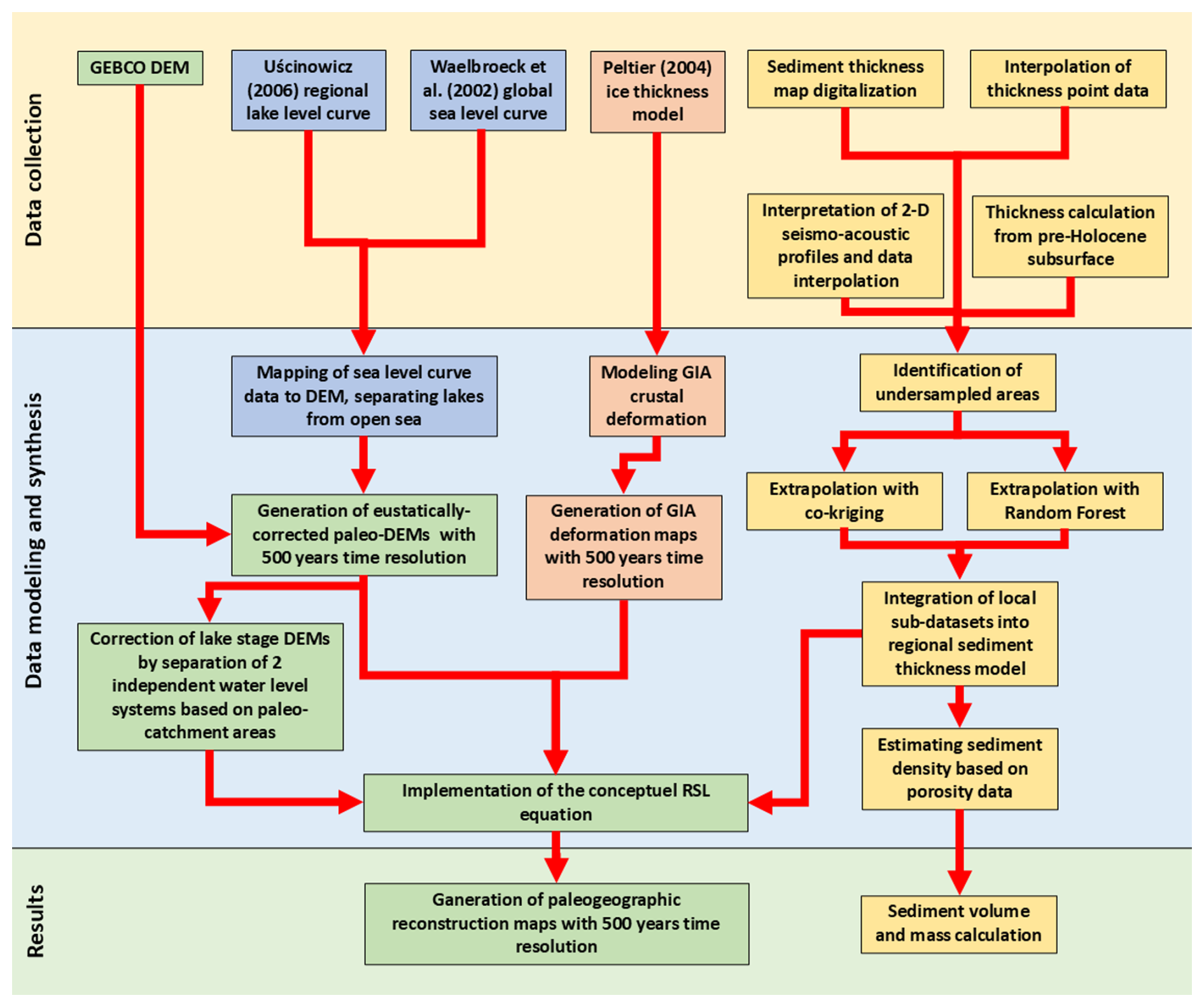
The reconstructed DEMs were plotted using the Golden Software Surfer 18 program. The software allows one to visualize surface relief with pre-defined spatial resolution (Bola and Kayode, 2014; Libina and Nikiforov, 2020), perform grid-on-grid mathematical operations (Liu et al., 2020a), interpolate the data (Gonet and Gonet, 2017; Razas et al., 2023; Yilmaz, 2007), and it therefore acts as a convenient, widely used tool in basin analysis (Covington and Kenelly, 2018; Grund and Geiger, 2011). The general workflow for data collection, synthesis, and interpretation is depicted in Fig. 2.

Figure 2 General workflow chart for data collection, synthesis, and interpretation.

3.1 Digital elevation model (DEM₀)

The present-day DEM₀ acting as a base for paleogeographic reconstruction was obtained from the General Bathymetric Chart of the Oceans (GEBCO) (Sandwell et al., 2002; Becker et al., 2009). The DEM for the Baltic Sea region spans 9.5–31° E in longitude and 52–66.5° N in latitude. The spatial resolution of the GEBCO grid is 15 arcsec (0.004167°×0.004167°) and was interpolated to our Baltic Sea grid (0.01°×0.01°). Maintaining the original resolution is unnecessary, as the eustatic and isostatic components were characterized by significantly lower resolution. Such transformation had negligible influence on the quality of the generated maps, allowing us in parallel to boost the map generation speed and save storage space.

3.2 Eustatic data (EC)

For the generation of the regional sea-level curve, a dataset by Waelbroeck et al. (2002) was used as a base. However, adjustment to the regional paleogeographic setting is needed. The Baltic water-level curve followed the Waelbroeck et al. (2002) data for the brackish marine stages, namely from 11.7–11 kyr BP (Yoldia Sea) and from 9.5 kyr BP until the present day (Littorina Sea) (Andrén et al., 2011). Knowing that, during the Ancylus Lake stage (11–9.5 kyr BP), the water level in the Baltic Sea basin was generally higher than that in the open ocean, a local water-level dataset of the southern Baltic region from Uścinowicz (2006) was applied to adjust the curve correspondingly. Even though the local relative sea-level curves are strongly influenced by the glacial isostatic adjustment (GIA; Andrén et al., 2002, 2011; Groh et al., 2017; Rosentau et al., 2012, 2021; Harff et al., 2017), the southern Baltic region is located near the isostatically neutral hinge line between uplift in the north and subsidence in the south (Statteger and Leszczyńska, 2023). Therefore glacial isostatic adjustment played a minor role in the estimation of the relative water level in the southern Baltic region. Such a feature allowed us to incorporate sea-level values of the Ancylus Lake from Uścinowicz (2006) into Eq. (2) as the “eustatic component”. Moreover, the lake phase of the Baltic region refers to two independent water-level systems: one for the Ancylus Lake and the other for the North Sea. The border between these two water bodies was set based on the paleo-catchment areas obtained using “Terrain Aspect” function in the Golden Software Surfer program on previously generated paleo-DEMs. In the lake phase, the water level in the Baltic Sea basin followed the curve in Uścinowicz (2006), whereas, in the North Sea, it followed the curve in Waelbroeck et al. (2002). These two curves are shown in Fig. 3.

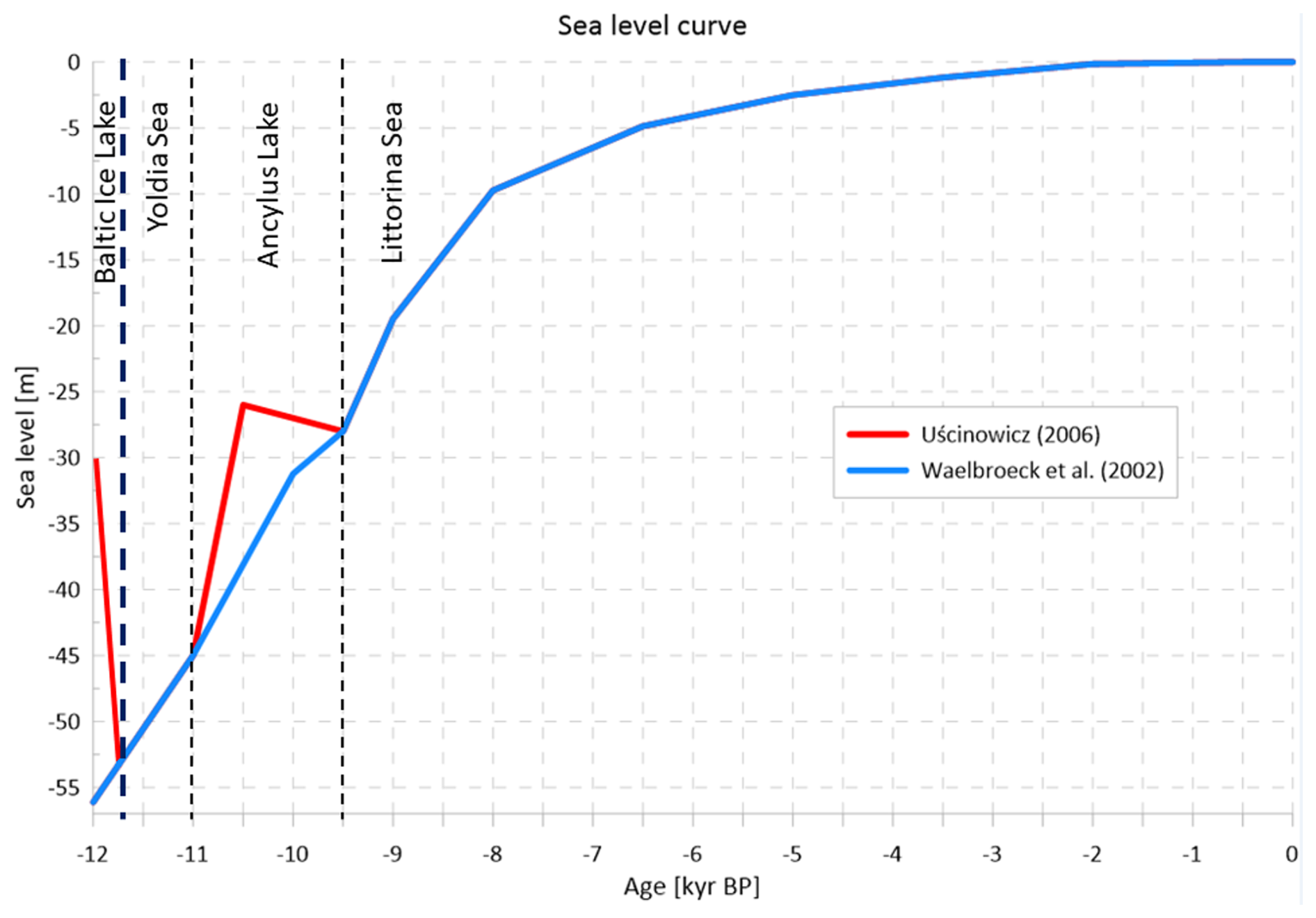
Figure 3 Holocene water-level curve for the Baltic region generated by a combination of Waelbroeck et al. (2002) and Uścinowicz (2006).

3.3 Vertical crustal movements – glacial isostatic adjustment (GIA) including a paleo-ice thickness model

The solid Earth's response to the changing surface loads of the vanishing Pleistocene ice sheets is known as glacial isostatic adjustment (GIA). This viscoelastic response comprises an instantaneous elastic and a delayed viscous component. GIA manifests in terms of deformations of the Earth's crust; changes in relative sea-level, i.e., sea level with respect to the Earth's deformable crust; and changes in gravitational potential (e.g., Peltier, 1998). The later originates from the redistribution surface masses, i.e., the melting of ice masses and the freshwater consequently added to the ocean, and from material in the Earth's mantle relocated as a reaction to the changing surface loads.

The decreased stress on the Earth's crust induced by the melting of the Laurentide ice sheet after the Last Glacial Maximum (LGM) about 21 kyr BP caused a crustal deformation which is still ongoing (Root et al., 2015). The crust is uplifting in regions formerly covered by ice. Crustal subsidence can be observed in regions surrounding the former ice cover known as the peripheral bulge (Steffen and Wu, 2011). This subsidence originates from the relocation of mantle material back to its original location in the Earth's interior underneath the region formerly covered by the ice (Vink et al., 2007). The crustal uplift is partly compensated by the additional water load stemming from the freshwater influx. However, the meltwater is unevenly distributed over the ocean according to the changing gravitational potential caused by the varying distribution of ice masses and by the water masses themselves. Thus, close to the melting ice sheets, a drop in relative sea level can be observed due to both the decreasing gravitational attraction of the ice and the uplifting crust.

The complex interaction between changing ice and water loads, their gravitational potential, and the induced crustal deformations is described in a gravitational self-consistent way by the sea-level equation (e.g., Farrell and Clark, 1976; Peltier, 1998). To solve the sea-level equation and model the GIA-induced vertical crustal deformation, we used the freely available software package SELEN (Spada and Stocchi, 2007). This software makes use of the ICE-5G ice load history (Peltier, 2004) to describe the spatiotemporal evolution of the ice sheets from the LGM until the present day at a temporal resolution of 1 kyr. A time interval of 500 years required for this study was achieved by assuming a linear trend between each millennium. Figure 4 depicts the ice thickness at the LGM (21 kyr BP) according to the ICE-5G load history as implemented by the SELEN software package. Cumulated crustal deformations are modeled starting from an equilibrium state at the LGM. Details of the applied model setup are provided in Groh and Harff (2023). The resultant GIA dataset was interpolated to our 0.01°×0.01° grid.

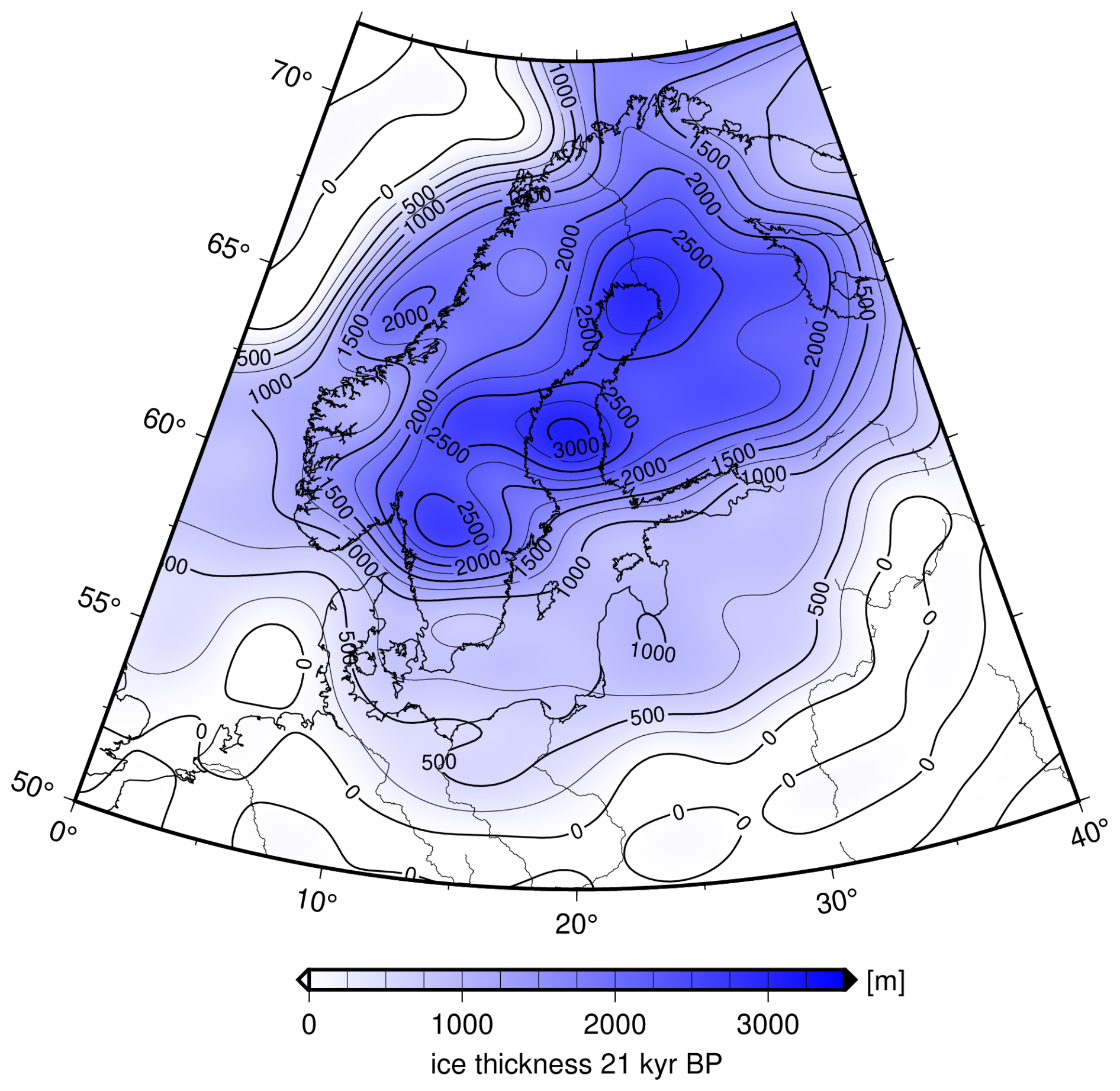
Figure 4 Present-day coastline and ice thickness at the Last Glacial Maximum (21 kyr BP) according to the ICE-5G ice load history (Peltier, 2004) as implemented by the software package of Spada and Stocchi (2007) after synthesizing its spherical harmonic representation to space domain.

3.4 Sediment thickness (SED)

The Baltic Sea basin is administrated by nine countries: Denmark, Germany, Poland, Sweden, Lithuania, Latvia, Estonia, Finland, and Russia. Due to the fact that no joint Holocene sediment thickness database is available, it is necessary to identify and merge various existing local datasets from publicly available sources. To generate a consistent regional sediment thickness model, eight local datasets were synthesized (Fig. 5). These sub-datasets were derived by six methods of data acquisition, including digitalization of isopach maps, recalculation of thickness from seismic reflector depth maps, interpretation of two-dimensional (2D) seismo-acoustic profiles and data interpolation with ordinary kriging, interpolation with ordinary kriging of point data from sediment cores, extrapolation using co-kriging, and extrapolation using a convolutional neural network (CNN). All sub-datasets were produced at 0.01°×0.01° resolution.

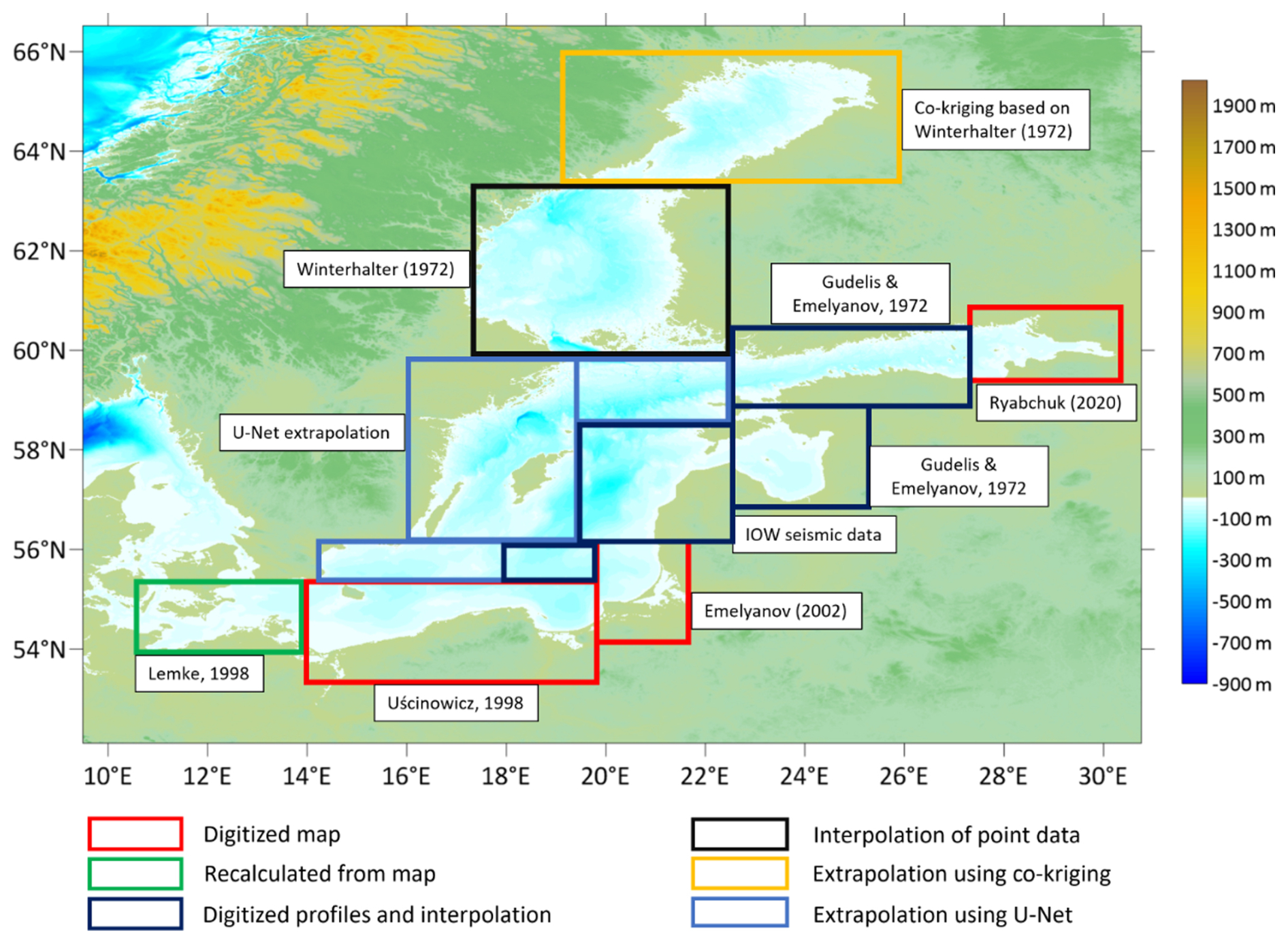
Figure 5 Map marking different types of data sources with generation of sediment thickness sub-datasets by digitalization of published Holocene isopach maps (red), recalculation of thickness from seismic reflector depth maps (green), digitalization of profiles and data interpolation (dark blue), interpolation of point data (black), and extrapolation using co-kriging (yellow) and convolutional neural networks (bright blue).

3.4.1 Southern Baltic region

The southern Baltic Sea area consists of German, Danish, Polish, Russian (Kaliningrad area), and Lithuanian coastal waters and is characterized by well-documented Holocene sediment thickness data with satisfactory quality. The sediment thickness model was generated as a result of merging three local-scale datasets. The German and Danish parts were covered by data derived from Lemke (1998). The depth of the top layer of glacial till corresponds to the Pleistocene basement, which was subtracted from the present-day DEM in order to estimate the Holocene sediment thickness. The sediment thickness data for the Polish waters were provided by Uścinowicz (1998), whereas data for the Russian (Kaliningrad area) and Lithuanian territories were retrieved from Emelyanov (2002). Due to slight differences in thickness values on the border between these two datasets, the values at the grid junction were averaged.

3.4.2 Central Baltic region

The central Baltic (Bornholm Basin, Eastern Gotland Basin, and surroundings) Holocene thickness grids were retrieved from 2D seismo-acoustic profiles collected by the Leibniz Institute for Baltic Sea Research Warnemünde (IOW), Germany (courtesy of Dr. Peter Feldens). In total, 240 seismic lines, collected between 2005 and 2009, were investigated. The Holocene basement corresponds mostly to the top of glacial till (Late Pleistocene-age, non-stratified seismic facies). The top of glacial till is a well-visible seismic reflector on most profiles, whereas the boundary between the BIL and the Yoldia Sea is difficult to discern in some profiles. Since the BIL belongs to the Late Pleistocene, the thickness for the Holocene sediment may be slightly overestimated in these profiles. A maximum local thickness of BIL sediments of up to 7 m is found in the deepest parts of the basins and diminishes towards the shallower areas according to Christiansen et al. (2002). Therefore, our estimated thickness of the Holocene sediment might be overestimated by ∼20 % in the deepest part of the basins, with the uncertainty decreasing towards the shallower areas. The seismic reflector corresponding to the pre-Holocene basement was exported as depth data points (shot points), transformed from the two-way travel time to metric units assuming a sound velocity in sediment of 1600 m s⁻¹, and further interpolated using ordinary kriging with nugget effect (Wackernagel, 2003). The obtained basement subsurface depth data were subtracted from the present-day DEM to generate the Holocene sediment thickness model.

3.4.3 Eastern Baltic region

Holocene sediment thickness data of the Gulf of Riga and the Gulf of Finland were generated based on profiles provided by Gudelis and Emelyanov (1976). Sub-datasets consisted of five N–S-oriented profiles connecting the edges of the Gulf of Finland and six profiles (four NW–SE-, one N–S-, and one W–E-oriented) across the Gulf of Riga. The reflector corresponding to the top of glacial till was digitized and exported as point data and then interpolated using ordinary kriging with nugget effect and subtracted from the present-day DEM. Thickness data covering the Russian part of the Gulf of Finland were derived from a digitized sediment thickness map by Ryabchuk et al. (2020).

3.4.4 Northern Baltic region

Holocene thickness data in the northern Baltic region are scarce because the area is undersampled. A mean post-glacial thickness dataset by Winterhalter (1972) consisting of 72 polygons (0.5°×0.5° resolution) located in the Bothnian Sea served as a base for interpolation. The central point of each polygon was exported as a data point and then interpolated using ordinary kriging. To fill the data gap in the severely undersampled northern part of the Bothnian Bay, data points of thickness from Winterhalter (1972) were used for extrapolation by co-kriging (Goovaerts, 1998; Myers, 1982, 1984). The co-kriging extrapolation method is commonly used in geoscience for areas where correlated measurements of multivariate variables are available (Belkhiri et al., 2020; Leenaers et al., 2020; Konomi et al., 2023). In the northern Baltic region, a two-dimensional variable consisting of a GIA-corrected paleo-bathymetry and thickness of Holocene sediments was used. The Pearson's correlation coefficient between the two variables is 0.52 in the measured point data, suggesting the feasibility of co-kriging-based extrapolation. Parameters of the corresponding semivariogram were determined using those grid nodes where data of both variables were available. These parameters allowed a co-kriging estimation of thickness data northward for undersampled areas.

3.4.5 Filling of data gaps

Machine learning was applied to fill the remaining gaps in the Holocene sediment thickness data. The areas with data gaps mainly include the central western part of the Baltic Sea (see Fig. 5). A convolutional neural network (CNN), namely a U-Net (Ronneberger et al., 2015), was built using PyTorch (Paszke et al., 2019). U-Nets have been proven to be robust and versatile tools for image and data analysis (Zhang et al., 2018; Liu et al., 2020b) and are superior to pixel-based methods such as random forest (Boston et al., 2022). In this study, four variables, namely the paleo-land surface morphology, the median grain size of surface sediments, and longitude and latitude values, were used to predict sediment thickness. The reason for adding the latter two variables is their relationship with the GIA (Fig. 4). The available data were randomly cut into 420 squares of 32×32 pixels, excluding the Gulf of Finland and the Gulf of Bothnia. The reason for excluding the two regions is because they differ substantially in geological, tectonic, and depositional environment from the central, southern, and southwestern parts of the Baltic Sea (Harff et al., 2017). This helps to reduce the error in the predictions. Of the 420 sub-datasets, 80 % were used for model training and 20 % were used for assessment of the model prediction. The input of the U-Net has the shape (32, 32, 4), and the output shape is (32, 32). The first layer consists of a double convolutional block performing 3×3 convolution with 64 output channels, padding, batch normalization, and ReLU activation. The training was performed with 100 epochs, and the mean squared error (MSE) was calculated as the loss function (torch.nn.MSEloss). Re-running the model with different random initializations and dropout yields different model results with the same general pattern but some local differences in sediment thickness. The result with the smallest value of MSE (6.1 m²) was chosen (Fig. 6). This corresponds to an average deviation from the validation to the measured data of 5.8 %.

3.4.6 Integration of sub-datasets

Each local Holocene thickness sub-dataset was integrated to one consistent regional grid with a resolution of 0.01°×0.01°. Small spatial gaps between the sub-datasets of thickness were linearly interpolated. In the case of a dataset not covering the coastline, the solution proposed by Miluch et al. (2021) was used by setting equidistant pinpoints characterized by 0-thickness values along the coastlines and included in the dataset. Such a solution allowed us to linearly extrapolate the thickness data between the grid points and the coastline to completely close the remaining data gaps. It is worth noting that the synthesized sediment thickness dataset does not cover the present-day land parts except for barrier islands that have been developed during the Holocene. Details on the data source, density, and interpolation and extrapolation techniques are listed in Table 1.

Table 1 List of sub-datasets of Holocene sediment thickness with information on gridding techniques along with primary data type and density.

3.5 Sediment budget analysis

Generation of the thickness map allows us to perform sediment budget analysis that helps identify sediment sources, sinks, and transport pathways. The grid was transformed from the geographic coordinate system to UTM projection to conduct volume calculation. Applied volume calculation algorithms include the trapezoidal rule, Simpson's rule, and Simpson's $\mathrm{3}/\mathrm{8}$ rule (Atkinson, 1989). Each method approximates different three-dimensional (3D) connection shapes between the data points, which slightly influence the calculated volume. Results from the algorithms were compared to assess the uncertainty. Sediment mass calculation requires information of sediment bulk density that is related to sediment particle density and porosity. Surface sediment porosity was calculated based on the present-day sediment grain size map of the Baltic Sea derived from the project Dynamics of Natural and Anthropogenic Sedimentation (DYNAS) (Bobertz et al., 2009; Harff et al., 2011) and application of the empirical formula from Endler et al. (2015) to link porosity to the median grain size. Knowing that the compaction rates of sandy and silty sediments are neglectable at a thickness scale of meters (Schmedemann et al., 2008), constant vertical porosity depending on the local grain size was assumed for the Holocene deposit. Pore volume was subtracted from the general volume. Knowing that Baltic Sea sediments are mainly clastic (Anthony et al., 2009), quartz with a density of 2.65 g cm⁻³ was used as the particle density. With the gridded data of porosity and sediment thickness and a constant particle density, both the overall mass of the Baltic Sea Holocene sediments and the annual rate of deposition averaged over the period are estimated.

3.6 Generation of paleogeographic maps

Having all the needed components described in Eqs. (1) and (2), namely the eustatic sea-level change, the spatial distribution of the GIA and the sediment depositional thickness, the present-day DEM₀ was transformed into a set of paleo-DEMs for the Baltic Sea, mimicking the paleogeographic evolution of the region with fine spatiotemporal resolution (see Supplement). The thickness of sediment deposition for each time slice (Δt=500 years) was subtracted from the total Holocene thickness assuming constant sediment accumulation rate.

4 Results

4.1 Holocene sediment thickness map

The integration of eight local-scale sediment thickness datasets with extrapolation methods allowed us to generate a regional Holocene sediment thickness map (Fig. 6). Several sites characterized by high sediment thickness were identified in the southern and central parts of the Baltic Sea, corresponding to depressions of sub-basins including the Arkona Basin, the Bornholm Basin, and the Eastern and Western Gotland Basin. The maximum deposition thickness reaches up to 36 m in the Arkona Basin and the Eastern Gotland Basin. Although regions of enhanced sediment accumulation are usually located in deeper basins, some shallower coastal areas also host locally confined deposits with thicknesses larger than 20 m. These include the central sections of the Gulf of Finland, the Gulf of Riga (both coupled with local bathymetry, as reported by Jakobsson et al., 2019), and the Gdańsk Basin. The thick Holocene deposit in the Gdańsk Basin is related to the formation of the Hel Peninsula that is driven by alongshore sediment transport (Uścinowicz, 2022). In contrast to the southern Baltic Sea, the Holocene sediment thickness in the northern Baltic Sea is relatively thin and mostly within 6 m. Such a feature may be related to the glacio-isostatic uplift resulting in a continuous reduction in accommodation space in the Bothnian Sea and the Bothnian Bay (Varela, 2015). The characteristics of seabed substrate of the northern Baltic Sea confirm the presence of glacial clay, hard-bottom complexes, and bedrocks covered by a thin layer of Holocene sand and gravel (Kaskela et al., 2012).

Figure 6 Regional Holocene thickness model derived from the synthesis of eight local sub-datasets and the application of three extrapolation methods (Table 1).

4.2 Sediment budget

Sediment volume calculated using the trapezoidal rule, Simpson's rule, and Simpson's $\mathrm{3}/\mathrm{8}$ rule provided nearly identical results (<0.001 % difference; see Supplement). The calculated total volume of Holocene sediment is 1.372×10¹² m³ in bulk. Subtracting the sediment porosity yields a zero-porosity sediment volume of 5.07×10¹¹ m³, corresponding to a total Holocene sediment mass of 1.34×10¹² t and an annual sediment accumulation of $\mathrm{1.15}\times {\mathrm{10}}^{\mathrm{8}}\mathrm{t}{\mathrm{yr}}^{-\mathrm{1}}$ (averaged over 11 700 years) in the Baltic Sea.

Potential errors in the estimation may originate from several sources, including porosity, grain density, vertical compaction, and an unclear boundary between the Late Pleistocene and early Holocene in the seismic profiles. The standard deviation σ of porosity is ∼0.15 according to the sediment samples analyzed by Endler et al. (2015). Applying the mean ±σ in the porosity data as the upper and lower estimates indicates a range between 0.82×10¹² and 1.87×10¹² t in the total sediment mass. Although the Holocene deposits mainly consist of silt and sand, the deeper basins (e.g., Arkona, Bornholm, and Gotland) are covered by a layer of a mixture of organic matter (up to 16 %) and clay (Leipe et al., 2011) that is subjected to the impact of vertical compaction. The thickness of such a layer can extend to several meters in the deep basins (Andrén et al., 2000; Ponomarenko, 2023). Assuming that the average thickness of this layer is 4 m (as indicated in a majority of sediment cores) in the basins, neglection of the vertical compaction results in an overestimation of the porosity by ∼10 % according to Schmedemann et al. (2008), corresponding to an underestimation of sediment mass of $\sim \mathrm{0.055}\times {\mathrm{10}}^{\mathrm{12}}\mathrm{t}$, which accounts for ∼4 % of the estimated mean total budget (1.34×10¹² t). As described in Sect. 3.4.2, an unclear boundary between Late Pleistocene and early Holocene sediment in the seismic profiles across the deep basins (e.g., the Gotland Basin) may lead to an overestimation of the Holocene sediment thickness by ∼20 % in the deepest part of the basins. The overestimation decreases toward shallower areas. A uniform overestimation of the deposition thickness in the basins by 20 % corresponds to a sediment budget of 1.1×10¹¹ t, which is ∼8 % of the estimated mean total budget (1.34×10¹² t). In summary, considering the uncertainties related to the major identified sources mentioned above in the estimation yields a total Holocene sediment budget ranging between 0.81×10¹² and 1.82×10¹² t, corresponding to an annual sediment accumulation rate between 0.69×10⁸ and $\mathrm{1.56}\times {\mathrm{10}}^{\mathrm{8}}\mathrm{t}{\mathrm{yr}}^{-\mathrm{1}}$.

4.3 Paleogeographic maps

A set of paleogeographic maps with a time interval of 500 years reflecting the evolution of the Baltic Sea region during the Holocene is provided in the Supplement, with maps for several periods marking a critical transition in the sea-level change shown in Fig. 7. To evaluate the paleogeographic maps, a reference is made to the widely used maps derived from proxy data interpretation (Fig. 1) produced by Andrén et al. (2011).

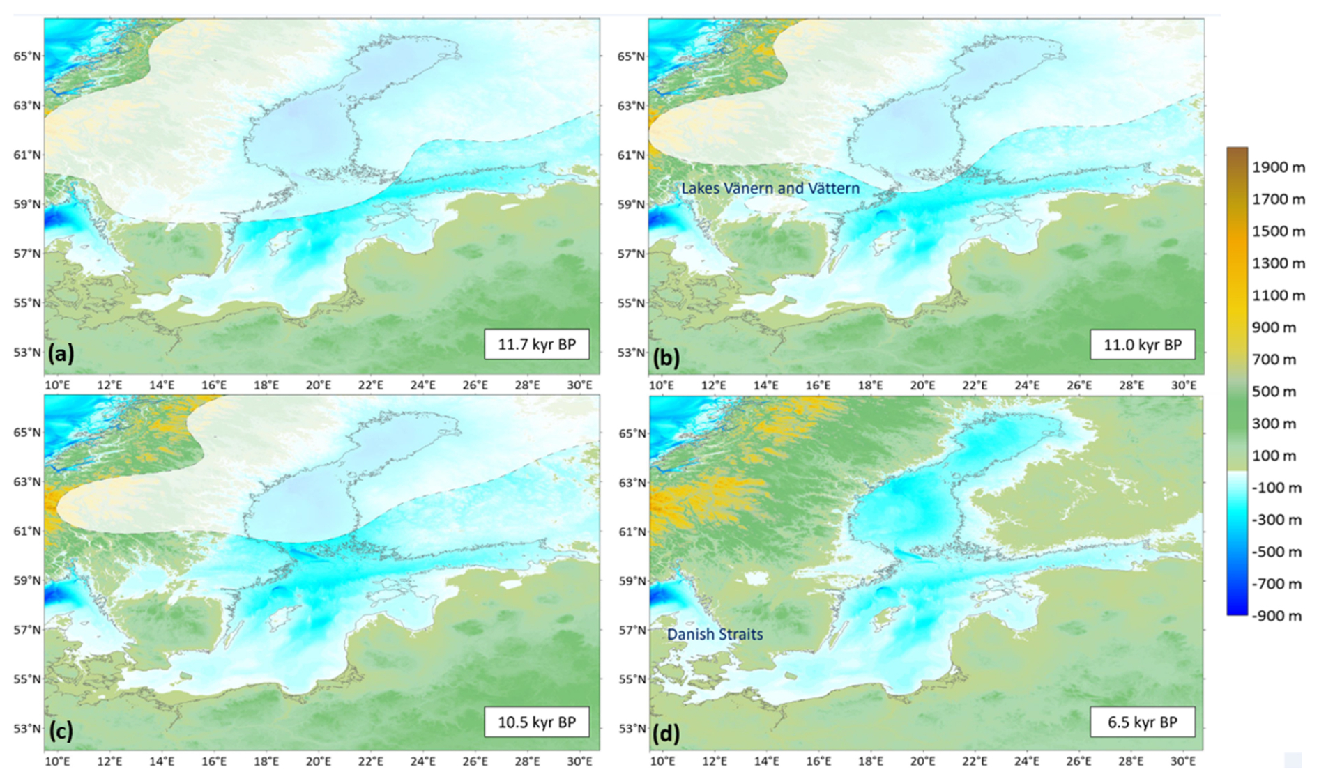
Figure 7 Reconstructed paleogeographic maps representing different stages of the Baltic Sea. Four exemplary maps are depicted here for comparison with the paleogeographic maps generated by Andrén et al. (2011). (a) Baltic Ice Lake/Yoldia Sea transition at 11.7 kyr BP; (b) Yoldia Sea (end of the brackish phase) at 11.0 kyr BP; (c) Ancylus Lake (maximum transgression) at 10.5 kyr BP; (d) Littorina Sea (most saline phase) at 6.5 kyr BP. The present-day coastline is depicted by the gray line, and the ice cover is indicated by the transparent mask.

At ∼11.7 kyr BP, a transition from the BIL to the Yoldia Sea stage occurred. At that time, a large part of the north of today's Baltic Sea basin was covered by the glaciers of the Fennoscandian Ice Sheet (FIS). The water level of the Baltic Ice Lake was dammed up to 25 m above the present-day sea level (Andrén et al., 2011) before the lake water made its way through the Central Swedish Depression on the southern border of the FIS and flowed into the paleo-North Sea basin in a drainage event in today's Kattegat (Fig. 7a). The rising sea level outpacing the moderate uplift of the mainland in the immediate vicinity of south of the ice margin in the Central Swedish Depression sustained a free exchange of water through a gate between the Baltic Sea and the North Sea for several centuries that marks a brackish marine phase called the Yoldia Sea stage (11.7–11.0 kyr BP). Both maps, the paleo-DEM shown in Fig. 7b and that of Andrén et al. (2011) shown in Fig. 1b, confirm the existence of such a gate. The maps clearly show the course of the inherent BIL drainage in the lowlands of the Central Swedish Depression through lakes Vänern and Vättern. This drainage course was near the margin of the FIS. According to Patton et al. (2017), Shaw et al. (2006), and Stokes et al. (2015), the continental ice front is not regarded as a stable line but rather consists of multiple glacial–fluvial channels between large ice blocks. The central Swedish lowland was characterized by such an environment, enabling the water flow between the Baltic Sea and the North Sea during the Yoldia Sea stage (Fig. 7a and b). During the Yoldia Sea stage (Fig. 7b), the sea level in the open North Sea and the water level in the Baltic Sea basin converged and lasted until ∼11.0 kyr BP. As the ice front continued to retreat northwards, the increasing uplift of Scandinavia outpaced the eustatic sea-level rise and closed the gate in the central Swedish lowland. The Baltic Sea consequently reverted to a freshwater environment, namely the Ancylus Lake, fed primarily by meltwater from the remnants of the FIS, which still covered the highlands of Scandinavia. The increasing flow of meltwater into the Ancylus Basin led to a rise in the lake level (so-called “Ancylus Transgression”) reaching a peak at ∼10.5 kyr BP and a subsequent drainage of the lake water into the paleo-North Sea (Fig. 7c). Different from the drainage through the central Swedish lowland in the later stage of the BIL, the freshwater outflow in the late stage of the Ancylus Lake moved to the south due to the increasing glacio-isostatic uplift of Scandinavia and took place through the area of today's western Baltic Sea, namely the Danish Straits. In the generation of the maps, we distinguished the water levels between the Ancylus Lake and the open North Sea from 11.0–9.5 kyr BP according to Uścinowicz (2006), which are shown in Fig. 3.

At ∼9.5 kyr BP, the one-way drainage from the Baltic Sea (Ancylus Lake) to the North Sea ceased due to a rise in the eustatic sea level which caught up with the water level in the Ancylus Lake (Harff et al., 2017), and the Littorina transgression enabled a free exchange between the Baltic Sea and the open North Sea again (Fig. 7d). Since then, the global sea-level change has dominated the hydrographic regime in the Baltic Sea. Glacio-isostatic movements of the region lead to persistent transgression in the south and regression in the north of the Baltic Sea (Harff et al., 2017). The paleogeographic setting at 6.5 kyr BP is illustrated by the map shown in Fig. 7d. A comparison with the map generated by Andrén et al. (2011) based on proxy data shown in Fig. 1c shows a general agreement in the reconnection of the Baltic Sea basin to the open North Sea and verifies our model result.

4.4 Validation of the paleogeographic reconstruction

An interplay between eustasy and spatially varied rates of isostatic rebound is mirrored in various local RSL curves. Reconstructed curves for all subareas of the Baltic Sea basin gathered by Rosentau et al. (2021) allowed us to locally assess our numerically modeled paleogeographic maps. All station data located along the eastern (Berglund, 2012; Hansson et al., 2018) and northern Swedish coast (Linden et al., 2006) and the Finnish coast (Glückert, 1976; Saarnisto, 1981; Mietinen, 2002) suggest a decreasing RSL since 11.7 kyr BP whereas stations on the southern Baltic coast mirror a consistent rising RSL that slows down and stabilizes after 6.0 kyr BP (Lampe and Janke, 2004, Lampe et al., 2011; Gelumbauskaite, 2009; Uścinowicz et al., 2011). Stations along the Latvian and Estonian coast (Grudzińska et al., 2013, 2014; Lougas and Tomek, 2013; Berzins et al., 2016) infer a generally decreasing RSL interrupted by the Ancylus transgression. The reported local RSL curves show discrepancy with our model results mainly for the initial stage between 11.7–10 kyr BP and afterward a general agreement (Fig. 8). The opposite patterns of RSL change between the northern and southern coasts gradually converge towards the central Baltic area, where eustatic and isostatic components neutralize each other. This is seen at the stations in Latvia and Blekinge (Sweden) which show a relatively flat RSL curve with small-scale variations (Damusyte, 2011; Rosentau et al., 2013; Habicht et al., 2017). Such a relatively stable RSL is reproduced in our results, albeit with discrepancy in the period between 11.7 and 10 kyr BP for the Blekinge station and between 11 and 8 kyr BP for the Latvia station (Fig. 8). A general agreement between our modeled RSL and local RSL curves compiled by Rosentau et al. (2021) and an agreement in the connection/disconnection between the open North Sea and the Baltic Sea basin described in the previous section validate the approach applied in this study.

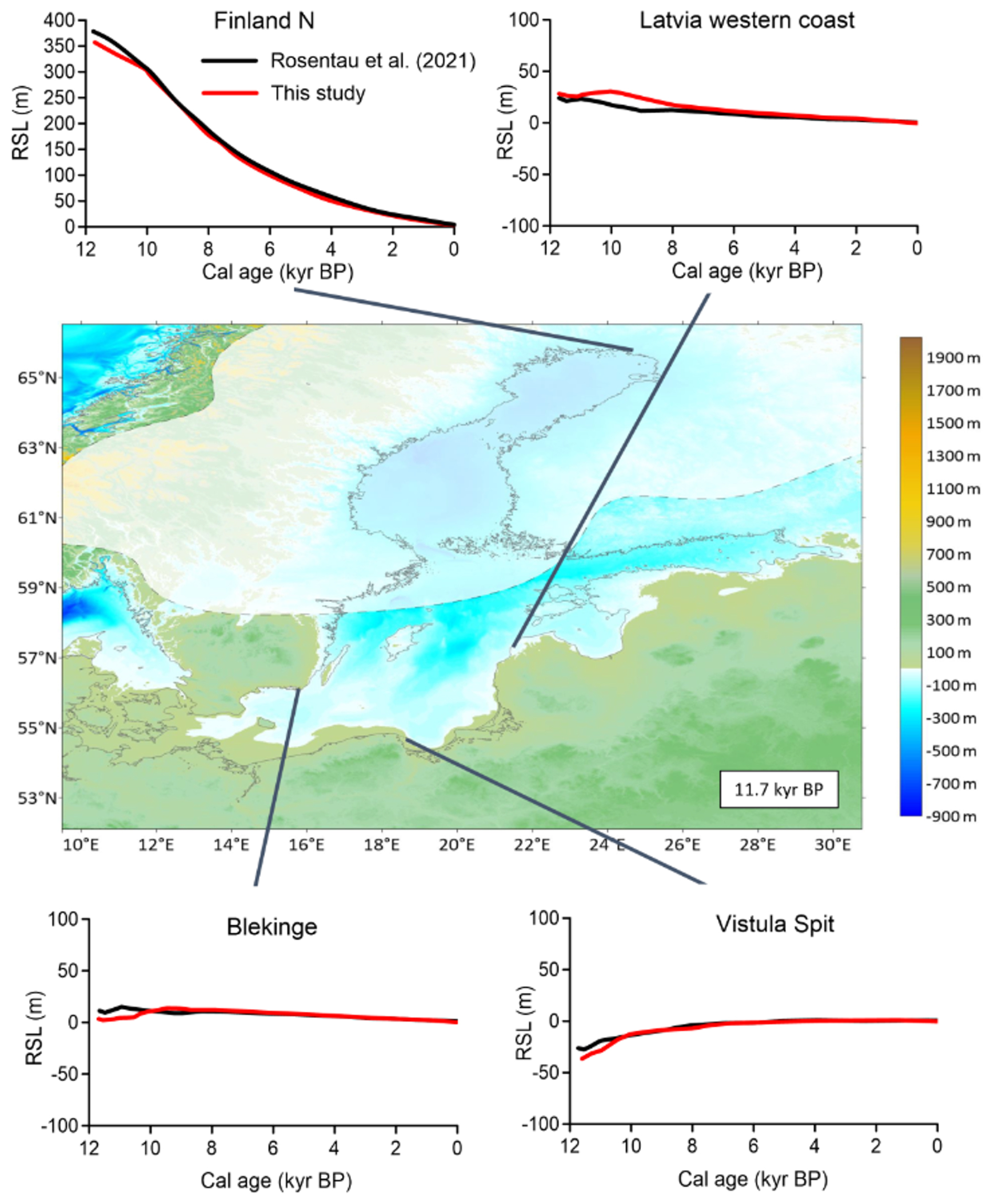
Figure 8 Comparison of our modeled RSL (red curves) and local RSL (black curves) derived from the ICE-5G model with 120 km lithosphere thickness by Rosentau et al. (2021).

5 Discussion

5.1 Comparison with existing reconstructions

The maps generated in this study are further assessed by comparison with existing local reconstructions. A comparison of RSL curves between those by Rosentau et al. (2021) and our results shows a general agreement except for the early Holocene period, as described in the previous section. In three stations, namely Finland N, Blekinge, and Vistula Spit, our results show a lower RSL at 11.7 kyr BP than those in Rosentau et al. (2021) adopting 120 km lithosphere thickness (Fig. 8). It should be noted that remarkable differences exist in the reconstructed local RSLs for the early Holocene period among the scenarios adopting different lithosphere thickness values as shown in Rosentau et al. (2021). As pointed out by Rosentau et al. (2021), the reconstructed curves using global ICE-5G and ICE-6G_C ice histories overestimate the RSL and fail to capture a mid-Holocene highstand ($\sim \mathrm{7.5}-\mathrm{6.5}\mathrm{kyr}\mathrm{BP}$) inferred from the proxy data in the transitional area. This overestimation seems to originate from an overestimation of ice loading in the ICE-5G model and especially in the ICE-6G_C model. Our modeled curves lie in the lower limit of the RSLs in Rosentau et al. (2021) and therefore may provide results closer to proxy data.

We also compared our modeled paleo-DEMs with the maps from Andrén et al. (2011) in a qualitative manner and identified a general consistency between the two sets of maps in the location of the gates between the Baltic Sea basin and the open North Sea along with the timing of their closing and opening (Sect. 4.3). Nevertheless, some local-scale differences are also seen between our results and the maps of Andrén et al. (2011), e.g., on the morphology of the Bornholm and Gotland islands. On the map of Andrén et al. (2011), both islands are shown to have emerged by 11.7 kyr BP. By contrast, our map shows that the island of Bornholm is still connected to the mainland and that the island of Gotland is largely submerged at that time. The shape of the coastline remains similar; however, a higher RSL in the southern part and a lower RSL in the western and eastern parts of the Baltic Sea are seen in Andrén et al. (2011) compared to our results. Such a difference may be attributed to the fact that the map of Andrén et al. (2011) still represents the late stage of the BIL when the water level was higher by ∼25 m in the Baltic Sea basin than in the North Sea, whereas our results correspond to the beginning of the post-drainage phase when the water levels of these two seas converged. For the maximum of the Ancylus transgression at 10.5 kyr BP, a state when the North Sea and the Baltic Sea are disconnected, a difference in the coastline location of the northern Baltic region between the two maps is seen. The difference indicates a lower RSL leading to the emergence of the West Estonian archipelago and Finland on the map of Andrén et al. (2011) compared to our results. Noteworthy is that, even though the difference in the coastline position seems to be huge, the difference in the elevation is relatively small (mostly within 10 m), suggesting that the land–sea transition in this part is highly sensitive to the change in RSL; therefore slight modification of isostatic or eustatic components may have a significant influence on the coastline position. Our reconstructed morphology of the Littorina Sea at 6.5 kyr BP is characterized by an open connection between the Baltic Sea and the North Sea through the Danish Straits, which persists today. In the reconstruction by Andrén et al. (2011), the Baltic–North Sea connection at 6.5 kyr BP exists via all three straits, being consistent with our results at that time. Some local-scale topographic structures, such as the shape of the straits, may vary between different reconstructions due to insufficient spatial resolution or data coverage. Similarly to earlier scenarios, the RSL in the northern and central parts of the Baltic Sea is generally lower on the map of Andrén et al. (2011) compared to our results.

An earlier effort in mapping Holocene sediment thickness in the Baltic Sea was made by Jakobsson et al. (2007). The mapping took place through assembling information from available sediment distribution maps and information retrieved from the Swedish Geological Survey's mapping archives, which unfortunately do not provide open access. The resultant map is characterized by relatively low spatial resolution and is limited to the southern and central parts (without the Bothnian Bay) of the Baltic Sea (Jakobson et al., 2007). A comparison between our map (Fig. 5) and that of Jakobson et al. (2007) shows a general agreement in the Bornholm Basin and along the Swedish coast near the Gotland Basin. However, there exists a large discrepancy in the thickness value in other basins (e.g., Arkona Basin, Gotland Basin) between the two maps. The thickness values in Jakobson et al. (2007) for these basins are much smaller than previous published values from Lemke (1998) and Uścinowicz (1998) focusing on these local areas. Despite a likely overestimation of the Holocene sediment thickness in the deep Gotland Basin, as pointed out in Sect. 3.4.2, integrated data from the difference sources within this study show more consistent patterns covering both deep basins and shallow coastal areas and therefore provide a more accurate distribution of Holocene sediment thickness.

5.2 Major source and sink terms in the Holocene Baltic Sea

A comparison of the annual sediment accumulation rate averaged over the Holocene with the present day's estimation by Porz et al. (2021) suggests that they are at the same order of magnitude for the SW Baltic Sea. The Holocene-averaged accumulation rate is $\mathrm{8.8}\pm \mathrm{4.1}\times {\mathrm{10}}^{\mathrm{6}}\mathrm{t}{\mathrm{yr}}^{-\mathrm{1}}$ in the SW Baltic Sea according to our data in this study. In the budget analysis done by Porz et al. (2021), the annual accumulation rate of fine-grained sediment in the SW Baltic Sea basins is between 5.5×10⁶ and $\mathrm{8.2}\times {\mathrm{10}}^{\mathrm{6}}\mathrm{t}{\mathrm{yr}}^{-\mathrm{1}}$.

Coastal erosion, namely erosion of the glacial till cliffs, serves as the main source that contributes at least 80 % of the annual deposition in the basins (Wallmann et al., 2022). Sediment supply from major central European rivers, namely the Oder, Vistula, Nemunas, Daugava, and Neva, is on the order of $\mathrm{1}\times {\mathrm{10}}^{\mathrm{7}}\mathrm{t}{\mathrm{yr}}^{-\mathrm{1}}$ (Porz et al., 2021; Pruszak et al., 2005; Lajczak and Jansson, 1993), with the largest contribution from the Vistula River ($\mathrm{0.16}-\mathrm{0.4}\times {\mathrm{10}}^{\mathrm{7}}\mathrm{t}{\mathrm{yr}}^{-\mathrm{1}}$). This indicates that the riverine sediment supply accounts for less than 10 % of the total Holocene sediment budget in the Baltic Sea. Biogenic production contributes to 4 %–15 % of the annual deposition budget (Wallmann et al., 2022; Porz et al., 2021). In addition, sediment input from the North Sea is estimated to be on the order of $\mathrm{1}\times {\mathrm{10}}^{\mathrm{6}}\mathrm{t}{\mathrm{yr}}^{-\mathrm{1}}$, contributing to 10 %–30 % of the annual deposition in the SW Baltic Sea (Porz et al., 2021). However, this input is almost negligible (accounting for ∼1 %) compared to the total annual accumulation rate in the Baltic Sea. The additional supply of sediment from melting ice cover in Scandinavia may occur during early Holocene stages. However, such a supply might also be negligible compared to the total Holocene sediment budget given that the Scandinavian mountains provide only a very small suspended sediment yield that is on the order of $\mathrm{1}\times {\mathrm{10}}^{\mathrm{5}}\mathrm{t}{\mathrm{yr}}^{-\mathrm{1}}$ (Lajczak and Jansson, 1993).

It is worth noting that our Holocene sediment thickness map is spatially confined by the present-day Baltic Sea coast. Although Holocene sedimentation may also occur on parts of the present-day mainland, especially on the northern Baltic coast when they were submerged, the deposited sediment was subjected to reworking when these parts became emerged and is therefore difficult to quantify due to lack of data. Moreover, the Holocene sediment thickness of the northern Baltic Sea and its coast is generally scarce (Fig. 6); therefore the omission of deposit on the mainland is considered to have a minor impact on the paleo-DEMs and the total Holocene sediment budget in the Baltic Sea.

5.3 Importance of integrating sediment dynamics in paleogeographic reconstructions

Depending on the regional or local setting, the individual impact of eustatic, isostatic/tectonic, and sediment dynamics on geographical and morphological development of marginal seas may vary significantly. The inclusion of sediment dynamics in paleogeographic reconstruction of coastal regions and continental shelves that are fed by significant terrestrial sediment input has a critical influence on the location of the paleo-coastline and general morphology of the seabed. This has been demonstrated in the paleo-reconstructions of the Beibu Gulf in the northern South China Sea (Xiong et al., 2020; Zhang et al., 2020), the Pearl River Delta and its estuary (Wu et al., 2010), the Mekong Delta and its adjacent shelf (Wang et al., 2024), the southwestern coast of the Bohai Sea (Liu et al., 2016), and the southern North Sea (Van der Molen and Van Dijck, 2000).

The integration of sediment dynamics is also important for understanding the evolution of large-scale sedimentary systems which are not directly fed by riverine sediment but are formed and/or shaped by sediment transport, such as barrier islands (Zhang et al., 2011a, 2014; Karle et al., 2021) and mud depocenters (Porz et al., 2021). This process is especially important for the evolution of the southern Baltic Sea, where various barrier islands have developed since the mid-Holocene, when the sea level approached a relatively stable level (Uścinowicz et al., 2011; Zhang et al., 2011b; Dudzińska-Nowak, 2017). It is worth noting that, although many paleogeographic reconstructions exist at local scales by considering sediment transport dynamics, our work represents the first attempt at a consistent reconstruction at a marginal sea scale. Comprehensive information of dated sediment thickness for a marginal sea such as the Baltic Sea is difficult to obtain, as most of the relevant datasets are derived locally, and it requires extensive effort to collect, integrate, harmonize, and synthesize such datasets and fill the gaps between them. A consistent paleogeographic reconstruction of a marginal sea, considering not only regional processes such as eustatic sea-level change and isostatic/tectonic movement but also sediment deposition, provides indispensable information on the historical development of the marginal sea, especially its coast.

A future challenge towards the improvement of paleogeographic reconstructions requires differentiation of sediment accumulation and erosion rates. Although the sediment accumulation rate may vary throughout the Holocene, we adopted a constant rate in this study due to poor data constraints. The reported rates were mostly derived based on the analysis of sparsely distributed sediment cores, and it is difficult to extrapolate a few tens of point data to the entire Baltic Sea. Therefore, more measurement data are needed to provide a sound database for extrapolation. Mass-balanced reconstruction methods have been proposed for the backstripping of depositional areas and backfilling of erosional areas at geological timescales (Hay et al., 1989; Feng et al., 2023). However, these are of high uncertainty for reconstructions at a millennial scale due to insufficient resolution in the seismo-acoustic profiles. An attempt to reconstruct the eroded coastal landscape in the mid-Holocene was performed by Zhang et al. (2014) at a local scale. The reconstruction was based on an extrapolation of the shape of present-day remnants of erodible coast by a fitted spline function using the morphology of the backland as a reference. Based on the identified major source and sink terms and on the associated transport pathways exemplified in this study, it might also be feasible to apply the same method to reconstruct eroded coasts at a centennial to millennial timescale.

6 Conclusions

This study presents a spatially high-resolution (0.01°×0.01°) paleogeographic reconstruction of the Baltic Sea basin, including the coastal evolution of the Baltic Sea for the Holocene since the end of the Baltic Ice Lake stage at 11.7 kyr BP. These data describe the surface structure of the study area, climate-induced eustatic sea-level change, the glacio-isostatic vertical movement of the Earth's crust, and the thickness of sediment deposition in the Baltic Sea basin. Local datasets of sediment thickness from open sources, including existing literature and data portals with public access, were compiled and complemented by numerical interpolation and extrapolation to generate a consistent regional map of Holocene sediment thickness for the entire Baltic Sea. The map shows that relatively thick Holocene sediments are deposited in the southern and central parts of the Baltic Sea, filling the sub-basins, including the Arkona, Bornholm, Eastern and Western Gotland, and northern central basins, with a maximum thickness of up to 36 m. In addition, some shallower coastal areas in the southern Baltic Sea also host localized deposits with a thickness of more than 20 m, mostly associated with alongshore sediment transport and formation of barrier islands and spits. In contrast to the southern Baltic Sea, the thickness of Holocene sediments in the northern Baltic Sea is relatively low, mostly less than 6 m. The total mass of Holocene sediment in the Baltic Sea is estimated to be between 0.81×10¹² and 1.82×10¹² t, corresponding to an annual sediment accumulation rate between 0.69×10⁸ and $\mathrm{1.56}\times {\mathrm{10}}^{\mathrm{8}}\mathrm{t}{\mathrm{yr}}^{-\mathrm{1}}$.

For the first time, the paleogeographic reconstruction of the Baltic Sea for the Holocene was achieved by a combination of crustal deformation (GIA), eustatic water-level change, and sediment thickness considering the disconnection of the paleo-North Sea and the easterly freshwater body during the Ancylus Lake stage. The model results are validated by comparison with field-based proxy data interpretation. This comparison improves the reconstruction of the hydrographic connection between the Baltic Sea and the North Sea in the marginal zone of the former Fennoscandian Ice Sheet. Our work thus represents a further step towards a consistent methodology to reconstruct the formation of marginal seas during transgression/regression cycles, including not only tropical and subtropical climate zones but also polar and subpolar marginal seas impacted by the regional dynamics of ice sheets.