Late Pliocene ice sheets as an analogue for future climate: a sensitivity study of the polar Southern Hemisphere

The Earth's ice sheets, including the Antarctic Ice Sheet (AIS), are critical tipping points in the climate system. In recent years, the potential future collapse has garnered increased attention due to its cascading effects, which could significantly alter global climate patterns and cause large-scale, long-lasting, and potentially irreversible changes within human timescales. This study investigates the large-scale response of the polar Southern Hemisphere (pSH; comprising the Southern Ocean and Antarctica (60–90° S)) to the geometric reduction in ice sheets to a reconstructed Late Pliocene (LP) extent and imposing increased greenhouse gas (GHG) forcing in the Earth System. Using the PRISM4D reconstruction, where ice sheets such as the West Antarctic Ice Sheet (WAIS) were significantly diminished, we conducted multi-centennial simulations with the EC-Earth3 model at atmospheric CO₂ concentrations of 280 and 400 ppmv. The simulation performed with LP ice sheet extent leads to a 9.5 °C rise in surface air temperature, approximately a 16 % reduction in sea ice concentration (SIC) over Antarctica and the Southern Ocean. These changes far exceed those driven by CO₂ increase alone, which result in a 2.5 °C warming and a 9.3 % sea ice decline. Additionally, both experiments deduce there is a reversal in sea level pressure (SLP) polarity with respect to pre-industrial (PI) patterns. Higher-than-normal SLP is present over Antarctica, and lower-than-normal SLP is present in the mid-latitudes, indicative of a negative phase of the Southern Annular Mode (SAM). This is supported by a weakening of the westerly jet, which in turn contributes to the formation of a fresh cap in the upper ocean, induced by the imposed climatic impacts of our sensitivity experiments. This overall freshening of the upper ocean increases stratification in the water column and prevents deep convection in the Southern Ocean, thus leading to the formation of the Antarctic Bottom Water (AABW), which is paramount for the ventilation of the global ocean. Overall, our findings suggest that, by increasing the atmospheric concentration of CO₂, the AABW is suppressed at a multi-centennial timescale; however, by reducing the ice sheet extent, compensatory mechanisms, involving an extensive salinisation of the ocean interior, trigger partial recovery of this water mass. This emphasises the non-linearity of the climate system, since consequences of reducing the ice sheets induce an amplified warming and freshening in the near-surface, whereas they induce opposing mechanisms in the deep ocean that significantly alter the dynamics of water masses that feed the AABW. By isolating the climatic response to ice sheet extent reduction, whilst holding other parameters fixed, this study offers critical insights into the mechanisms driving atmospheric and oceanic variability around Antarctica and their broader implications for global climate dynamics. Here we provide a unique, targeted approach, specifically focusing on the direct impact of ice sheet retreat on regional climate.

1 Introduction

The Earth's ice sheets, including the Antarctic Ice Sheet (AIS hereafter), are pivotal components of the climate system. Their high albedo reflects a significant portion of solar radiation, thereby cooling surrounding regions and playing a critical role in regulating global air and sea surface temperatures (SSTs). In addition, these ice sheets influence atmospheric and oceanic circulation at various scales, modulating rates of sea ice and deep-water formation and the wind regime across different oceanic basins (Clark et al., 1999). However, the stability of these ice sheets is currently at risk due to climate-change-driven enhanced surface and basal melting, with melting rates projected to intensify in the following decades (Pollard et al., 2015; Song et al., 2025).

Projections indicate that accelerated ice sheet loss will have far-reaching implications for global climate dynamics (Naughten et al., 2023; Greene et al., 2024; Buizert et al., 2018). These changes are likely to disrupt critical processes such as deep-water formation and the contribution of the Southern Ocean to global heat transport and carbon sequestration (Cai et al., 2013; Menviel et al., 2023). Understanding these risks is critical, as potential ice sheet collapse could trigger cascading climate feedbacks, leading to irreversible and long-lasting changes within human timescales.

Palaeoclimate records offer unique insights into the behaviour of these ice sheets during past warm periods, such as the Last Interglacial (LIG; ∼127 ka (kiloyears)) in the Pleistocene (Steig et al., 2015) and the Late Pliocene (LP; $\sim \mathrm{3.3}\times {\mathrm{10}}^{\mathrm{6}}$ years ago) (Naish et al., 2009; Kim and Crowley, 2000), when the ice sheets were significantly smaller than today. Using these periods as analogues, we can better understand how ice sheet dynamics influence oceanic and atmospheric processes in climates warmer than today, which can offer valuable lessons for predicting future climate behaviour as the Earth continues to warm.

However, as the LIG entails orbit-induced changes in insolation with respect to the modern climate (Otto-Bliesner et al., 2017), palaeoclimate insights from the Late Pliocene are increasingly used as analogues for future warm climate states, offering critical context for how Earth's climate system may respond to elevated CO₂ levels while at similar orbital configuration. The period was characterised by atmospheric CO₂ concentrations broadly comparable to present-day values, estimated at 350–450 ppmv (Haywood et al., 2016b). Global mean surface temperatures were 2–4 °C higher than pre-industrial (PI), with amplified warming at high latitudes. In the Southern Hemisphere, evidence suggests substantially reduced AIS extent, particularly the West Antarctic Ice Sheet (WAIS), and the retreat of marine-based sectors in East Antarctica (Dolan et al., 2018). Southern Ocean sea ice was likely seasonally absent or greatly reduced, accompanied by displaced westerly winds and changes in Antarctic Bottom Water (AABW) formation, with implications for Antarctic climate feedbacks and ice–ocean interactions. The combination of near-modern greenhouse gas (GHG) concentrations, polar amplification, reduced AIS extent, and reorganised Southern Ocean circulation makes the Late Pliocene a valuable palaeoanalogue for projected future change. Polar amplification ratios for the period have been estimated at around 2.3 (de Nooijer et al., 2020), closely aligning with future projections ranging between 2.11–2.76 depending on the chosen scenario (Xie et al., 2022; Pörtner et al., 2022). Both Chandan and Peltier (2018) and Lord et al. (2017) demonstrate how bridging LP knowledge and future projections improves our understanding on how sensitive the Earth's climate is to various forcings. Simulating the climate of the Late Pliocene is a core component of the Pliocene Model Intercomparison Project (PlioMIP) (Haywood et al., 2016a, 2022), which facilitates international multi-climate model comparisons for the Pliocene epoch (Haywood et al., 2010). Contributions from PlioMIP have been integral to the Intergovernmental Panel on Climate Change (IPCC) 5th (IPCC, 2013) and 6th Assessment Reports (Gulev et al., 2022). By providing insight into analogous climate forcings, the Late Pliocene offers a unique framework for understanding the long-term stability of the AIS and its impact on the Southern Ocean dynamics in a warming world.

However, existing work on the LP as a warm-climate analogue heavily focuses on Arctic processes, demonstrating the significance of surface albedo feedbacks involving the Greenland Ice Sheet (GrIS) retreat when considering future climate change (Power et al., 2023), identifying which key oceanic gateways amplified LP Arctic warming (Feng et al., 2017) and may do so again. Additionally, by understanding Pliocene polar amplification (Lunt et al., 2012; de Nooijer et al., 2020), more accurate projections can be made for amplification in a prospective warming world. In the Southern Hemisphere, the role of the AIS in modulating future climate is gaining attention (Weiffenbach et al., 2024), although significant uncertainties remain in understanding the Southern Hemisphere response to changing ice sheets, including mechanisms driving Southern Ocean stratification, AABW formation, and coupled atmosphere–ocean feedbacks specific to Antarctica.

Addressing these gaps is critical for constraining the sensitivity of the Antarctic climate system to sustained elevated greenhouse gas forcing. In this study, we replace the modern ice sheet mask of the EC-Earth3 model with that of the Late Pliocene reconstruction provided by the Pliocene Model Intercomparison Project phase 3 (PlioMIP3; Haywood et al., 2024). We perform three sensitivity experiments applying modern and LP ice sheet masks under two CO₂ concentrations (280 and 400 ppmv), whilst not modifying any other model boundary condition representative of the pre-industrial (1850 CE) Earth's geography. This approach allows us to assess the sensitivity of the climate system to changes in ice sheet extent and varying CO₂ concentrations, using ice sheet conditions of the past as an analogue for the future. Our work offers a unique contribution by isolating the impact of surface reflectivity changes associated solely with the reduction in ice sheet extent, independently of topographic or vegetation feedbacks and without freshwater inputs, allowing us to better quantify the role of the AIS in modulating Antarctic climate and Southern Ocean circulation. Our goal is to uncover the key mechanisms and processes that could profoundly influence Earth's future climate, environment, and societies.

2 Model configuration and experiment setup

2.1 Model configuration

We use the low-resolution configuration of the EC-Earth model, EC-Earth3-LR, an Earth system model (ESM) developed collaboratively by the European research consortium EC-Earth. The EC-Earth model has flexible configurations that allow the inclusion or exclusion of various climate processes, making it a versatile tool for a wide range of climate studies (Döscher et al., 2022). EC-Earth3 integrates several key components, including the atmospheric model IFS cycle 36r4, the land surface module HTESSEL, the ocean model NEMO3.6 (Madec, 2008), and the sea ice module LIM3 (Vancoppenolle et al., 2012), all coupled via the OASIS3-MCT coupler (Craig et al., 2017). IFS and HTESSEL have a horizontal linear resolution of TL159 (1.125°), and the ocean and sea ice components (NEMO and LIM) have a nominal resolution of 1° (Döscher et al., 2022).

The low-resolution configuration was selected to significantly reduce computational costs and because it has been extensively validated in both modern and palaeoclimate studies, showing robust performance in simulating the climates of past warm periods such as mid-Holocene, Last Interglacial, and Late Pliocene (Zhang et al., 2021; Chen et al., 2022; de Nooijer et al., 2020; Han et al., 2024). These simulations have provided valuable information that has been integrated to major model intercomparison projects, such as the Paleoclimate Model Intercomparison Project phase 4 (PMIP4) and the Pliocene Model Intercomparison Project phase 2 (PlioMIP2) (Haywood et al., 2020, 2024). Our setup allows us to conduct multi-centennial simulations and various sensitivity experiments, being particularly suited for exploring slow processes in the deep ocean, which are central to the goals of this study. Such processes include changes in stratification, overturning circulation, and AABW formation in response to altered climate forcing. Overall, the EC-Earth3 model has consistently demonstrated its effectiveness in capturing key climate dynamics, including temperature variability, heat fluxes, and other essential aspects of the Earth's system. This capability facilitates a more comprehensive understanding of the impacts of natural and anthropogenic forcing on the global climate system (Koenigk et al., 2013; Döscher et al., 2022; Cao et al., 2023).

2.2 Experiment setup

To investigate the impacts of varying ice sheet extent and CO₂ concentrations in the polar Southern Hemisphere (pSH), we performed a series of sensitivity experiments, displayed in Table 1. The experiment design is based on the Core and Tier 2/Extension experiments as outlined in the Pliocene for Future protocol of PlioMIP2 and PlioMIP3 (Haywood et al., 2016a, 2022). These experiments also follow the PlioMIP2 naming convention in which the experiments with modern ice sheet extent are labelled E and the Late Pliocene ice sheets are labelled Ei, followed by their atmospheric CO₂ levels. In our simulations, the experiment E280 comprises the CO₂ concentration reconstructed for the pre-industrial period (280 ppmv), while the experiments E400 and Ei400 employed the reconstructed CO₂ concentration of the Late Pliocene (400 ppmv). All simulations were started in parallel after branching off from a quasi-equilibrated PI spinup spanning 800 years to ensure consistent baseline conditions and that any changes observed in the simulations are due to the perturbation and not model drift. We defined quasi-equilibrium as a global surface air temperature trend of less than 0.05 K per century. Thus, the E280 experiment represents our pre-industrial control simulation, which is a core experiment of PlioMIP2/3, while E400 and Ei400 represent our sensitivity experiments, being within the Tier 2 experimental design of PlioMIP2 and continuing as optional but pivotal experiments in PlioMIP3 (Haywood et al., 2020, 2024). Specifically, the primary purpose of the E400 experiment is to clarify how an elevated CO₂ level with respect to PI, without other boundary condition changes, affects climate, a process usually referred to as forcing factorisation, which isolates CO₂-driven climate change from other palaeoclimate forcings. Conversely, Ei400 focuses on the combined impact of CO₂ and ice sheet extent change. Here we define the polar Southern Hemisphere as our domain of study, which includes the entire Southern Hemisphere from 60–90° S. To ensure consistency across all simulations, modern vegetation, as simulated for the year 1850 CE, was held fixed by disabling the offline LPJ-GUESS dynamic vegetation model (Chen et al., 2021). The final 200 years of model output is used for analysis of the mean state, with the pre-industrial control (E280) simulation serving as a baseline for comparison with the sensitivity experiments.

Table 1 The Core and Tier 2 Pliocene for Future protocol experiments conducted. PI refers to pre-industrial conditions, and LP refers to the Late Pliocene. The terminology is from Haywood et al. (2016a).

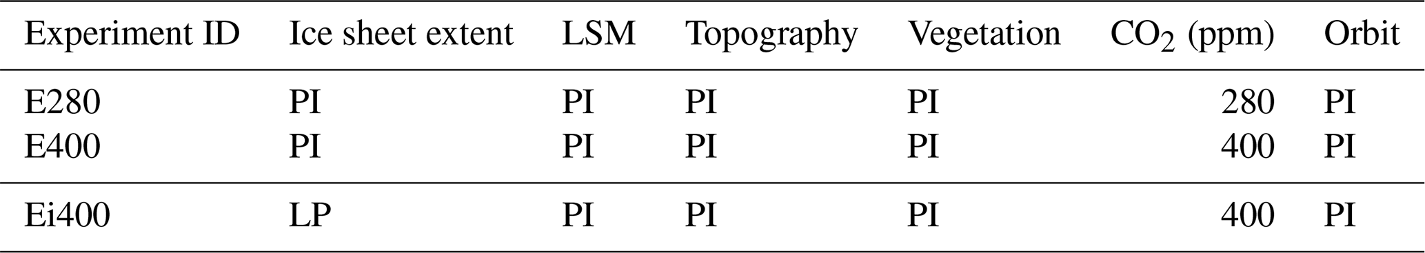
The protocol for our pre-industrial (PI) simulation follows the framework of Eyring et al. (2016) for the Coupled Model Intercomparison Project version 6 (CMIP6) piControl experiment. Ice sheets, land geography, topography, and vegetation are all unmodified from the model. GHG concentrations for CO₂, CH₄, and N₂O are 284.3 ppmv, 808.2, and 273.0 ppbv, respectively. For orbital parameters, eccentricity is set at 0.016764, obliquity is set at 23.549, and perihelion – 180° is set at 100.33.

The aim of these sensitivity experiments is to unveil the isolated impact of LP ice sheet extent to the climate of the polar Southern Hemisphere, without introducing confounding factors. To achieve this, we modify only the ice sheet mask to represent LP ice sheet extent while retaining pre-industrial albedo values and topography in the model. The LP AIS reconstruction was originally developed using the high-resolution British Antarctic Survey Ice Sheet Model, integrated with climatologies from the Hadley Centre Global Climate Model (Hill et al., 2007; Hill, 2009), utilising PRISM2 boundary conditions (Dowsett et al., 1999). The reliability of the AIS extent is further supported by the results of PLISMIP, which evaluated the dependencies of the ice sheet model for the warm period of the Late Pliocene using 30 different models (Dolan et al., 2012). Figure 1 provides a visual comparison of the modern and LP ice sheet extent. LP GrIS reconstruction is provided for PlioMIP2 (Haywood et al., 2016a) and based on 30 modelling results from PLISMIP (Dolan et al., 2012). Power and Zhang (2024) provide more detail, including spatial configuration of the LP GrIS and associated climatic impacts of modifying the GrIS in the polar Northern Hemisphere.

Figure 1 Comparison of the (a) modern and (b) LP Antarctic ice sheet extent in white, as provided by PLISMIP. Superimposed is the modern coastline of the Antarctic continent.

In our sensitivity experiments, the LP ice sheet masks were interpolated to the EC-Earth IFS grid and substituted into the initial condition referred to as the snow-depth field. In IFS, ice sheet presence is defined as grid cells with snow depth >10 m. By altering this field, we therefore reclassify those cells as exposed land or ocean in the LP experiments. The snow scheme in EC-Earth3 (based on ECMWF's HTESSEL land surface model) treats snow as perennial when snow depth exceeds a threshold 0.5 m of water equivalent, assigning a fixed high albedo and preventing further accumulation, effectively acting as a proxy for ice sheets. When snow depth is below this threshold, snow is considered seasonal and surface albedo is calculated as a weighted average between snow albedo and underlying surface albedo, reflecting seasonal snow cover variability (Döscher et al., 2022; Balsamo et al., 2009). In our experiments, the AIS orography is retained, but, in regions where snow depth falls below the perennial threshold, seasonal snow processes dominate, allowing accumulation and melt with seasonally varying albedo. All other initial and boundary conditions were held fixed at PI values, including the prescribed surface albedo fields, orography/elevation, GHG concentrations, aerosol fields, ocean boundaries, and soil and vegetation distribution, together with their modified albedo properties. Additionally, no freshwater hosing was applied.

This experimental design therefore isolates the climatic response to the geometric removal of ice cover under fixed pre-industrial albedo and topography. Areas that are ice-covered in PI but ice-free in LP retain the model's default PI surface properties for that grid cell type (bare land or ocean), rather than adopting LP-specific albedo or vegetation reconstructions. This design allows us to focus on the first-order radiative effect. By doing so, we isolate the radiative effect of land ice loss, how the change in surface reflectivity influences the local and regional energy balance, and the resulting dynamical response, including how these changes affect atmospheric circulation, wind patterns, and ocean feedbacks within the model framework. This controlled experimental design avoids confounding influences from additional forcings, such as changes in vegetation, soil moisture, or orography, which may otherwise obscure the direct climatic impact of ice retreat. In this way, the experiment acts as a valuable idealised sensitivity test that serves as a baseline for understanding the isolated role of ice sheet retreat on Southern Hemisphere climate dynamics.

3 The polar Southern Hemisphere response to increased CO₂ and LP ice sheets

The interactions between the atmosphere, cryosphere, and ocean are crucial in understanding the influence of increased atmospheric CO₂ concentrations and reduced ice sheet extent on climate feedbacks in the polar Southern Hemisphere.

3.1 Changes to temperature, albedo, and sea ice concentration (SIC)

In the E400 scenario (400 ppm CO₂, relative to E280), the average Antarctic surface air temperature rises by 2.51 °C. The warming is most pronounced in two specific regions that we refer to as “hotspots”, the Weddell (75° S, 50° W) and Ross (73° S, 160° W) seas, with temperatures increasing by up to 6 °C in the Weddell Sea and by 5 °C in the Ross Sea (Fig. 2a). Changes to albedo (Fig. 2c) are primarily confined to these two regions, with the most significant decrease (up to 20 %) occurring in the Weddell Sea, extending between the coastline and 60° S and clustered to the Weddell gyre. A smaller area of albedo decline (10 %) is observed west of the Ross Sea. Sea ice loss replicates these patterns surrounding the hotspots. The largest sea ice decline occurs to the east of the Weddell Sea (Fig. 2e) and is clustered to the coastline moving eastward, and a smaller area of sea ice loss is found west of the Ross Sea. More moderate warming occurs across the majority of the remaining area, with generally less than 2 °C increase over the interior of Antarctica and less than 1 °C at the periphery of East Antarctica. This is accompanied by virtually no changes in albedo. A localised cooling of 1–2 °C is observed in the Southern Ocean between 62° S, 160° W–160° E, where a small loss in albedo is also displayed (Fig. 2c).

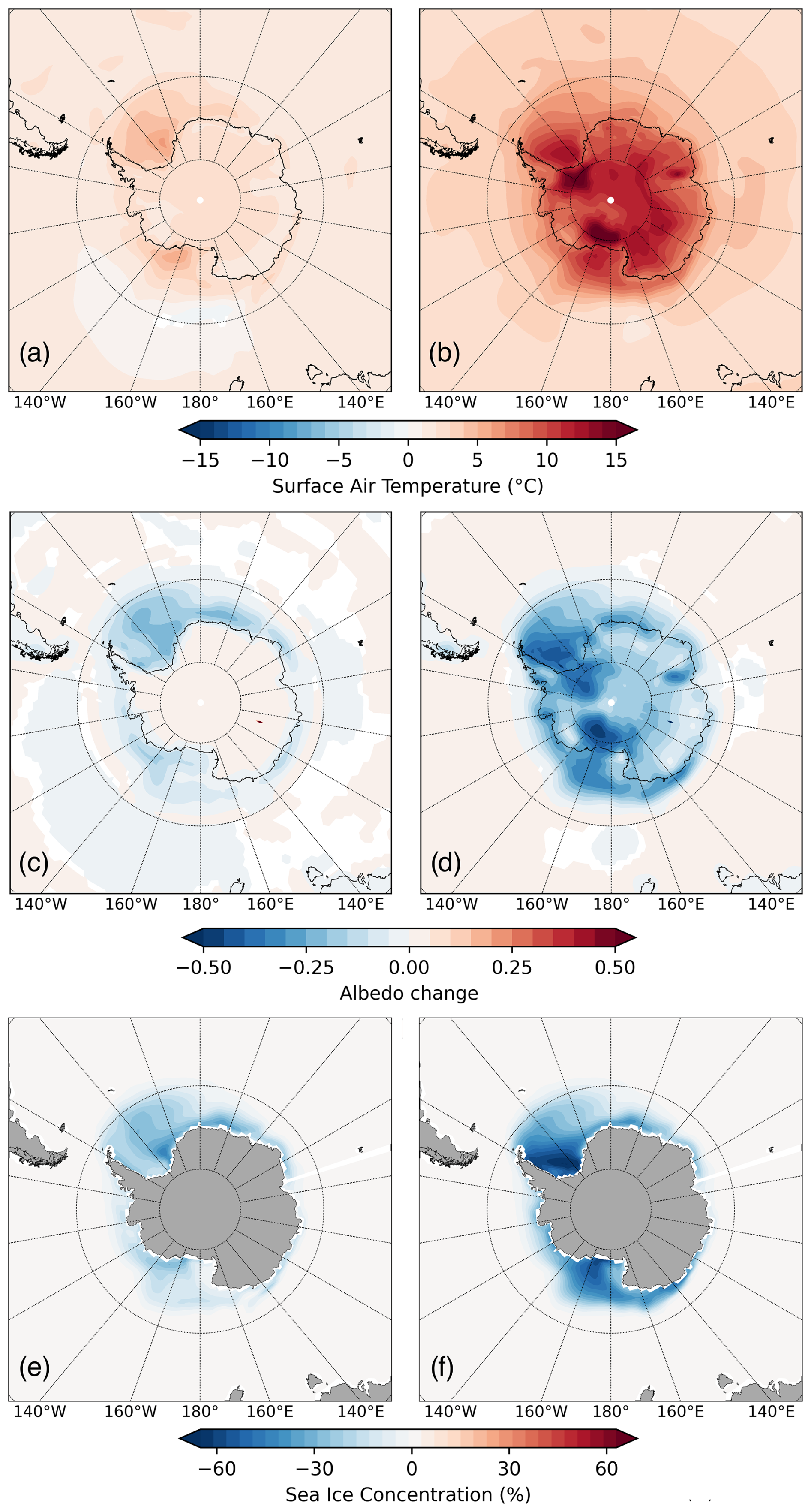
Figure 2 Temperature, albedo, and sea ice concentration (SIC) variables from the only increased CO₂ level experiment and combined CO₂ and LP ice sheet extent, compared with the PI control. (a) E400-E280 surface air temperature, (b) Ei400-E280 surface air temperature, (c) E400-E280 albedo, (d) Ei400-E280 albedo, (e) E400-E280 SIC, (f) Ei400-E280 SIC. Only results statistically significant at the 95 % confidence level are displayed.

In contrast, with LP ice sheet extent (Ei400 relative to E280), warming is much greater than in E400, with the near-surface air temperature over Antarctica increasing by an average of 9.49 °C. The warming hotspots shift further inland, with temperatures rising by over 17 °C inland from the Ross Sea (81–83° S, 180–155° W) and up to 16 °C inland from the Weddell Sea (81–83° S, 20–35° W) (Fig. 2b). The Ross and Weddell seas themselves experience warming of up to 12 and 13 °C, respectively. The most substantial albedo declines also occur at these inland hotspots, with a decline of more than 50 % inland of the Ross Sea, whilst the Ross Sea itself experiences a 30 % decrease. There is an albedo reduction of 40 %–50 % inland of the Weddell Sea, which extends into the Weddell Sea itself (Fig. 2d). Sea ice losses are consequently the most drastic in these locations, with a decline of over 65 % in the Weddell Sea and 60 % in the Ross Sea. Moreover, extensive areas of sea ice loss are observed extending eastward from the Weddell Sea and westward from the Ross Sea.

Over the interior of Antarctica, warming reaches 11–12 °C, decreasing towards the eastern coastline where temperatures increase by 6–7 °C. In Ei400, albedo changes are not confined to regions affected by ice sheet change, and there is an overall albedo decline of 20 % across the Antarctic interior, with decreasing severity toward the eastern coastline. There is a small hotspot showing a pronounced loss of 30 %–40 % on the east coast (75° S, 60–70° E). Additionally, albedo decreases of up to 30 % are observed along the coastline at 0–10° E and 140–160° E. This widespread albedo reduction is a result of the interplay of climate feedbacks that likely include changes in cloud cover, atmospheric temperature, and moisture transport influencing the radiation balance and surface reflectivity.

3.2 Changes to regional atmospheric circulation patterns

As the surface temperature rises due to the abrupt change in radiative forcing applied through our experiments, the subsequent shifts in climate create significant feedbacks that can influence large-scale atmospheric circulation, particularly the Southern Annular Mode (SAM). SAM is the leading mode of atmospheric variability in the Southern Hemisphere, characterised by fluctuations in the strength and position of the westerly winds encircling Antarctica (Marshall, 2003). It has a large influence on pSH climate, as the wind regimes over this region modulate sea ice and deep-water formation, along with other climate patterns (Morioka et al., 2024). Therefore, understanding how it responds to increased CO₂ concentrations and ice sheet changes is vital. Here we derive the SAM mean state of the sensitivity experiments (Fig. 3a, b, and c) by applying empirical orthogonal functions (EOFs) to the sea level pressure (SLP) field and extracting its first mode. SAM variability in the form of a time series spanning the last 200 simulation years (Fig. 4) was extracted through the first principal component of the EOF (PC1) and standardised.

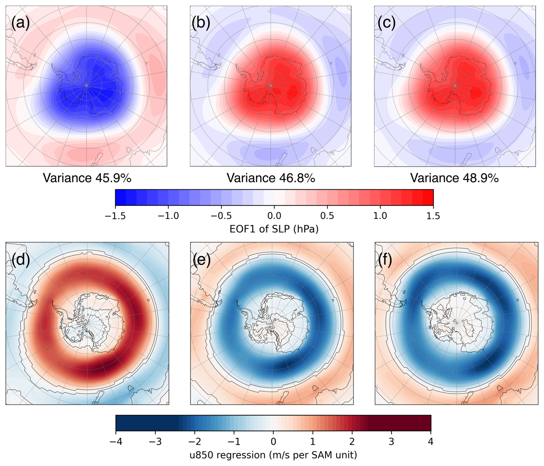
Figure 3 The Southern Annular Mode mean state as the first EOF of the SLP in hPa for the (a) piControl, (b) E400, and (c) Ei400 experiments, with the percent of variance explained by EOF1 notated for each. Regression of the austral summer (DJF) 850 hPa zonal wind onto the leading SAM principal component for (d) E280, (e) E400, and (f) Ei400. Colours indicate the regression coefficient per SAM unit. Black contours denote statistically significant values (p<0.05). Austral summer (DJF) is used as the SAM signal, as it is typically strongest during this period, with the stratospheric polar vortex remaining strong and the westerly jet well defined.

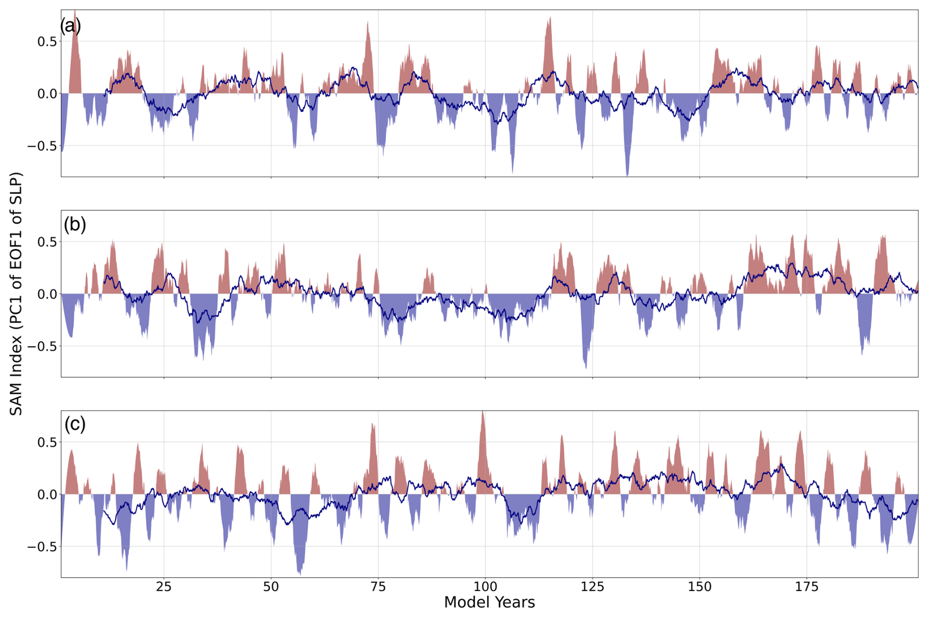
Figure 4 Time series of the Southern Annular Mode (SAM) index for (a) E280, (b) E400, and (c) Ei400 experiments, calculated as the standardised principal component (PC1) of the leading empirical orthogonal function (EOF1) of monthly mean sea level pressure (SLP) south of 20° S. A Savitzky–Golay filter with window of 61 is applied, smoothing the index over 5 years either side, with a 10-year running mean overlaid.

In E280, Fig. 3a reveals an atmospheric structure characteristic of a positive SAM phase, with lower-than-normal SLP over Antarctica (90–60° S) and higher-than-normal SLP in the mid-latitudes. Regression of austral summer (December–January–February, DJF) 850 hPa zonal wind onto the leading SAM principal component (PC1) shows the strengthening of mid-latitude westerlies, whilst easterlies strengthen to the north of the Antarctic Polar Front (APF; Fig. 3d), reflecting the poleward shift in the mid-latitude westerly jet during positive SAM phases (Marshall, 2003). The PC1 reiterates (Fig. 4a) the overall positive phase, with a slight positive central tendency (median 0.04) and marginally more positive months than negative (Table 2). A more positive SAM phase is typically associated with cooler temperatures over Antarctica in summer, such as those established in the E280 simulation, as stronger westerly winds act as a barrier to warm air transport from lower latitudes (Thompson et al., 2011).

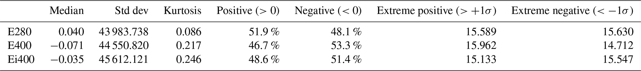
Table 2 Summary statistics – mean, variability (std), kurtosis, occurrence percentages of positive/negative and extreme events – describing the temporal behaviour of the first principal component (PC1) representing the SAM index in each experiment. Standard deviation and kurtosis are based on non-normalised data, and all other statistics are based on normalised data.

Under increased CO₂ forcing (E400), there is a reversal in EOF polarity. Higher-than-normal SLP is present over Antarctica, and lower-than-normal SLP is present in the mid-latitudes (Fig. 3b), indicative of a negative SAM phase. Mid-latitude Southern Ocean winds show strong negative anomalies (Fig. 3e), indicating an equatorial shift in the westerlies, thereby reaffirming the negative SAM phase. The PC1 time series (Fig. 4b) has a slight negative central tendency (median −0.07) and more negative months than positive. A negative SAM phase is associated with higher air temperatures across Antarctica and often leads to reduced sea ice formation that is triggered by katabatic winds in the pSH (Doddridge and Marshall, 2017). This, in turn, reduces the upwelling of cold deep-ocean water onto the Antarctic continental shelf, further reinforcing this negative feedback.

Combining CO₂ with LP ice sheet extent results in the same large-scale atmospheric structure as in E400, characterised by a negative SAM phase (Fig. 3c). The PC1 time series (Fig. 4c), however, demonstrates a behaviour closer to neutral in Ei400 than in E400, with a very small negative median (−0.03) and the most even split of negative to positive months out of the three experiments (Table 2). Additionally, Ei400 displays the largest raw variability (in units of the original PC1), potentially indicating a more chaotic and less stable SAM pattern.

3.3 Sea surface and deep-water formation sensitivity to modified boundary conditions

As evidenced in the previous section, the modified boundary conditions that were imposed in our experiments have significant implications for processes occurring in the near-surface atmosphere. Consequently, the sea surface and the ocean interior of the pSH are also affected. In E400, where we solely increase the atmospheric CO₂ concentration, the surface ocean exhibits similar warming patterns to the atmosphere (Fig. 2a), albeit at a much lower magnitude. Figure 5a shows an overall warming along the path of the Antarctic Circumpolar Current (ACC), particularly within 45–55° S and through the Brazil–Malvinas Confluence (BMC), along with warming hotspots in the Weddell and Ross seas that are advected eastward through the ACC. Additionally, the Pacific upper-ocean cooling exhibited in Fig. 5a is in close agreement in both magnitude and location with the region where atmospheric cooling occurs. In Ei400, sea surface warming (Fig. 5b) agrees even more consistently with the change in near-surface atmospheric temperature (Fig. 2b). The warming hotspots confined to the Ross and Weddell seas and the Adélie Coast also remain, with the same pattern of eastward advection of warm waters as in E400, although with SST increasing up to 5 °C in the Weddell Sea.

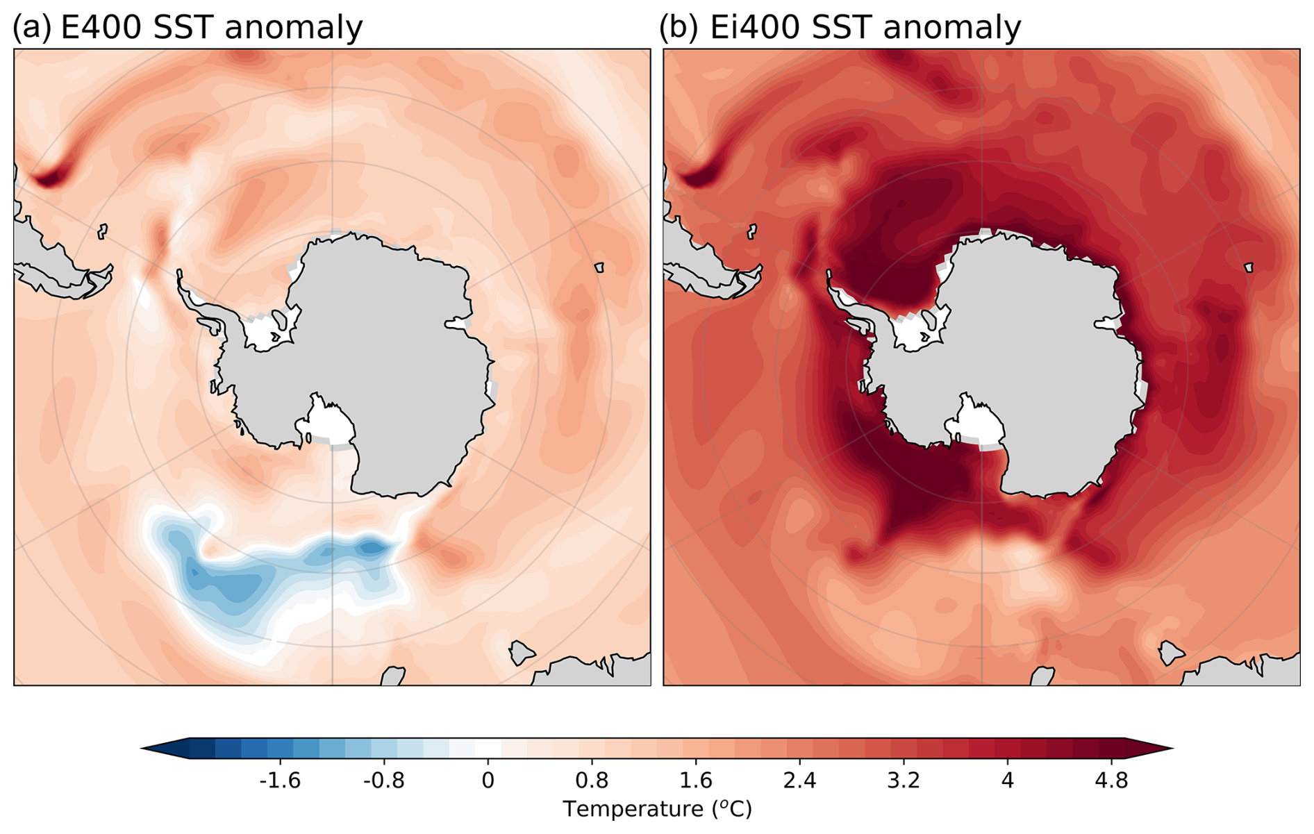
Figure 5 Anomaly of the sea surface temperature (°C) in (a) E400 and (b) Ei400 in relation to E280. Only results statistically significant at the 95 % confidence level are displayed.

With warming of the Earth's surface leading to an extensive sea ice melt (Fig. 2e and f), the surface layer of the Southern Ocean undergoes substantial freshening around the Sea Ice Zone (SIZ), which is highly sectorised. In E400 (Fig. 6a), the Bellinghausen and Davis seas exhibit the highest freshening, whereas the region encircling the APF (north of 55° S), the wind-driven outcrop of the Circumpolar Deep Water (CDW) in the Weddell gyre, and some parts of the Ross Sea exhibit upper-ocean salinisation. Conversely, with the stronger reduction in sea ice concentration that is imposed by reducing the ice sheet extent (Ei400), the surface freshening of the Southern Ocean is amplified (Fig. 6b), while the salinisation in the outcrop region of the CDW, in the Ross Sea, and outside the APF remains, albeit at a much reduced magnitude.

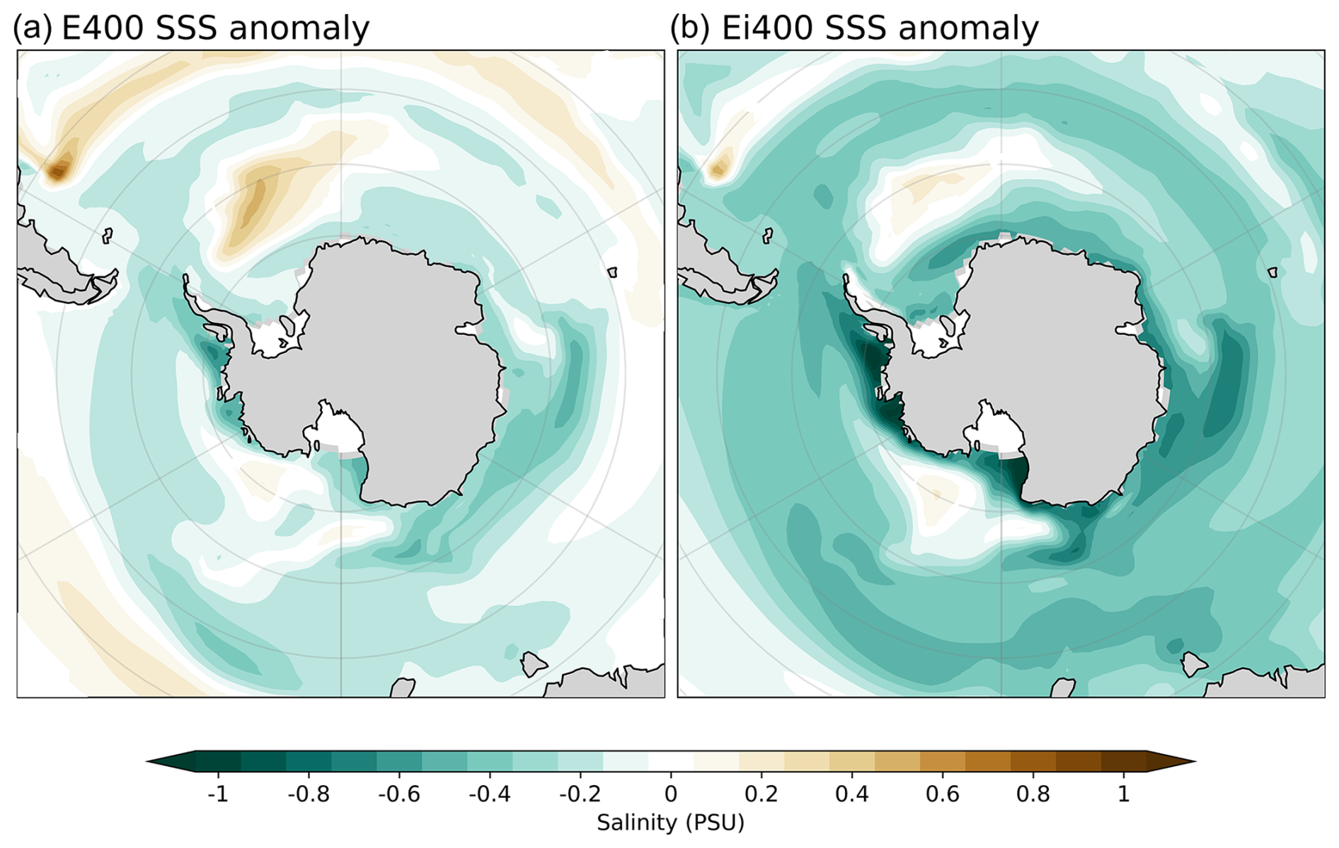
Figure 6 Anomaly of the sea surface salinity (PSU) in (a) E400 and (b) Ei400 in relation to E280. Only results statistically significant at the 95 % confidence level are displayed.

The combined effect of upper-ocean warming and freshening with weaker wind regimes within the APF (Fig. 3e and f) also affects the distribution of these thermohaline properties in the water column. Within the limit of the polar Southern Hemisphere, at 60° S, both E400 and Ei400 experiments exhibit the development of a fresh cap in the upper ocean that by itself increases the stratification of the water column (Fig. 7a and b) with respect to the pre-industrial climatology. As the westerlies weaken concomitantly, the stratification is sustained throughout the simulation, which further isolates the surface ocean. Moving down from the upper ocean, in E400 (Fig. 7a), the entire water column exhibits a uniform warming and salinisation during the runtime that is consistent with the higher sectorisation of areas that experience cooling (warming) and freshening (salinisation).

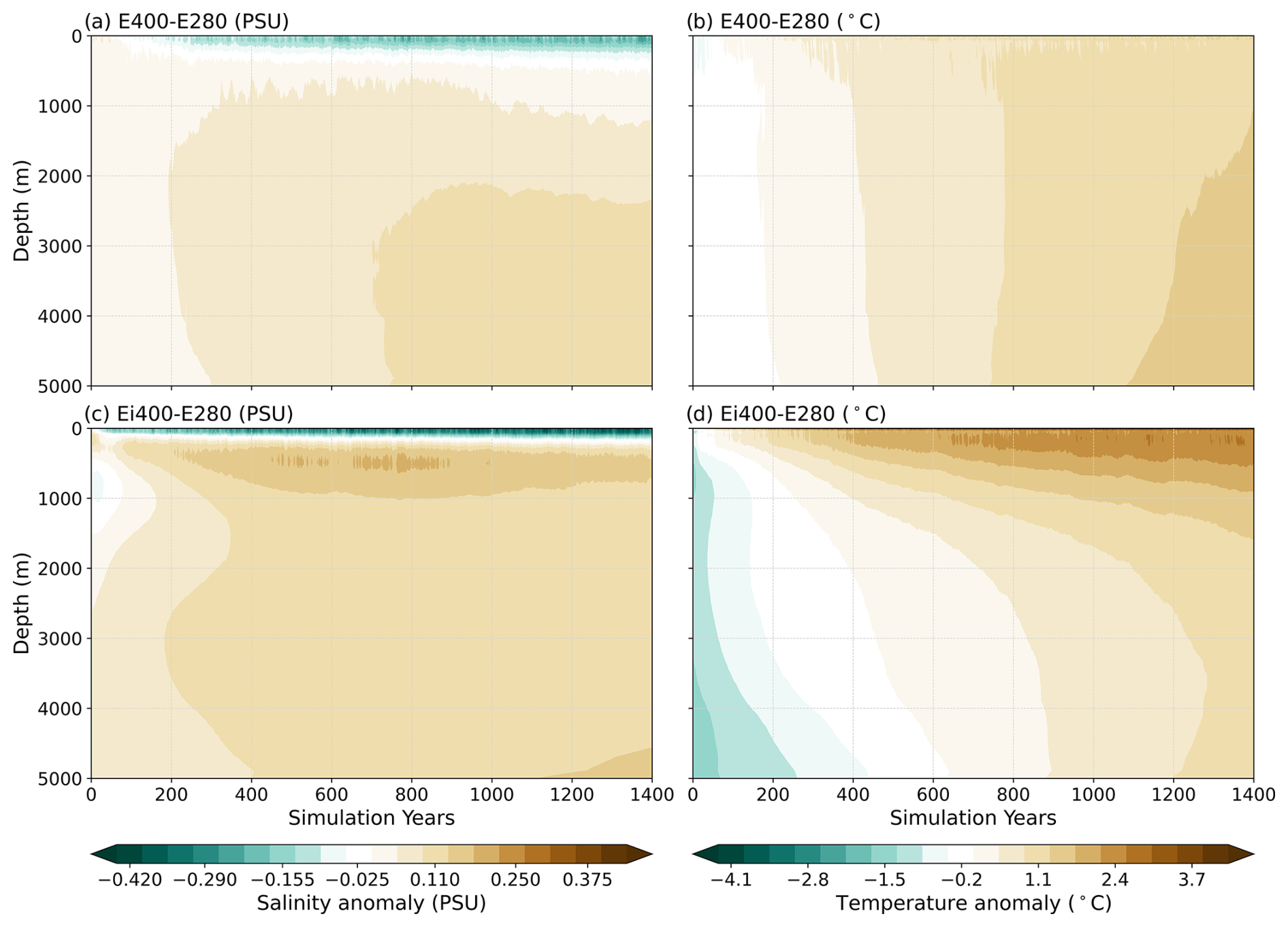
Figure 7 Hovmöller diagrams of salinity (a, b) and temperature (b, d) anomalies at 60° S, relative to the E280 average at the same latitude, for E400 (a, b) and Ei400 (c, d).

In Ei400 (Fig. 7b), however, the upper ocean experiences warming and freshening, whereas the subsurface undergoes warming and salinisation down to the intermediate layer (∼1000 m). This indicates an increase in stratification and a subsequent isolation of the ocean interior that allows its stronger salinisation in comparison to E400, especially at deep and abyssal depths. This likely occurs as a combined effect of the stronger stabilisation of the upper ocean, further reinforced by even weaker westerlies (Fig. 3f) and the entrainment of salty water masses through the intermediate layers of the Southern Ocean. Additionally, the abrupt forcing that is introduced by reducing the ice sheet extent in Ei400 results in an initial cooling of the ocean interior of about 3 °C, which offsets the degree of deep ocean warming in this simulation, when compared to E400. Therefore, in comparison to the pattern revealed in Fig. 7a, in Ei400, the Southern Ocean interior (surface) undergoes more salinisation (freshening) and less (more) warming.

As the changes in the sea surface temperature and salinity, which are amplified in Ei400 with respect to E400, impose contrasting effects in the ocean interior, the Southern Ocean Meridional Overturning Circulation (SMOC) undergoes a major shift (Fig. 8), particularly with respect to the strength of the AABW, which is essential for the ventilation of the global ocean (Orsi et al., 1999). Firstly, the SMOC reveals two major cells in E280: a clockwise cell that represents the northward flow of surface waters and the return flow of deep and intermediate waters that upwell at around 60° S and an anticlockwise cell that represents the northward flow of the AABW towards Indo-Pacific and Atlantic basins (Talley et al., 2016). In E400, the clockwise cell deepens and the AABW is significantly weakened from 8–2 Sv. In Ei400, on the other hand, the clockwise cell weakens and shoals, while the AABW exhibits a slight strengthening of about 2 Sv.

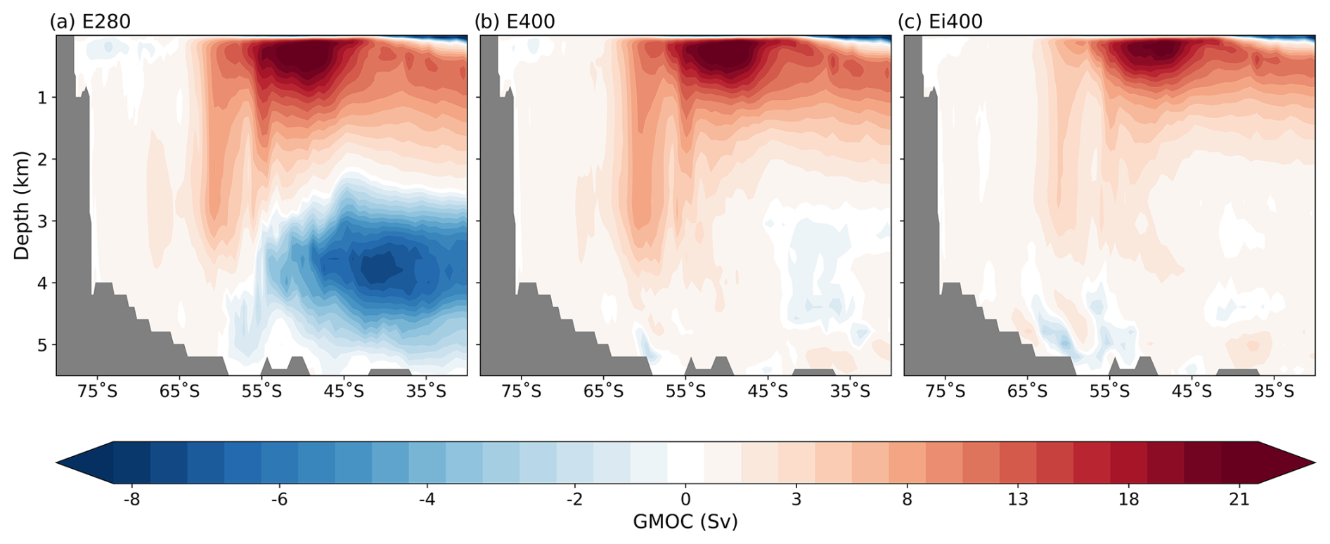
Figure 8 Southern Ocean MOC for the (a) E280, (b) E400, and (c) Ei400 experiments averaged over the last 200 years of the simulation.

Considering the mean state of the last 200 simulation years, we therefore see that the AABW undergoes extensive weakening in both sensitivity simulations. Such sustained weakening is consistent with the picture of freshening and warming of the upper ocean displayed in Fig. 7 but not completely consistent with the picture of salinisation of the deep ocean. To evaluate the strength and variability in AABW formation in our experiments during runtime and gain more insights into the overall state of abyssal overturning in the Southern Ocean, we derived an AABW index that consists of the absolute value of the minimum overturning south of 60° S and below 500 m depth (adapted from Zhang et al., 2019). Note that we exclude the upper 500 m from the index to isolate the water column comprising the subsurface to abyssal layers from the upper ocean and avoid capturing its high-frequency variability. The AABW index (Fig. 9) shows that, even though Fig. 8b and c indicate a similar pattern of AABW weakening in both sensitivity experiments, the evolution of the AABW strength shows a sustained weakening in E400 and a partial recovery in Ei400, particularly after simulation year 700. Additionally, in both sensitivity experiments, the variability in the AABW is significantly reduced with respect to E280. Such behaviour indicates that enhancing the atmospheric CO₂ concentrations, accompanied by massively reducing the extent of ice sheets, triggers compensatory mechanisms to the initial AABW suppression, likely involving salinisation of the deep and bottom ocean, as suggested in Fig. 7.

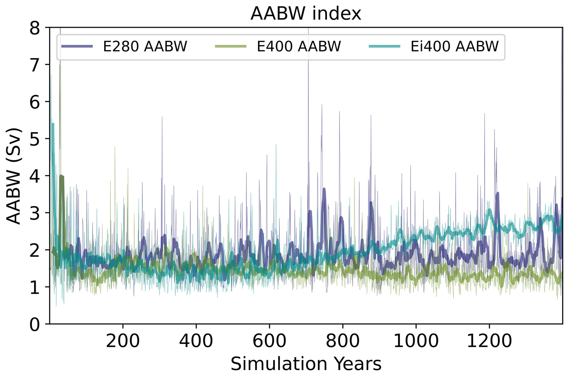
Figure 9 Time series of the Antarctic Bottom Water formation index for experiments E280, E400, and Ei400, calculated as the absolute value of the minimum global streamfunction of the pSH domain (60–90° S and below 500 m depth, adapted from Zhang et al., 2019).

Furthermore, as the AABW formation is a complex process that is not yet fully understood and receives contribution from other masses formed in the Southern Ocean, particularly in the deep ocean (Pardo et al., 2012), the insights gained from Figs. 7–9, indicate that the underlying mechanism for the partial recovery of the AABW in Ei400 is a combination of the changes in salinity and temperature that occur in the water column, isolated through the weakened wind regime (Fig. 3f), and the interplay between the water masses in the Southern Ocean that are directly affected by these changes. The overall change in water mass density and thermohaline properties can easily be visualised through a temperature–salinity (T–S) diagram (Fig. 10). In the figure, we highlight major water masses that are formed in the Southern Ocean and directly contribute to, or are the main product of, deep-water formation that is exported to the global ocean, including Antarctic Surface Water (AASW), Antarctic Intermediate Water (AAIW), Circumpolar Deep Water (CDW), High Salinity Shelf Water (HSSW), and Antarctic Bottom Water (AABW). In this sense, AASW, CDW, and HSSW are contributors to AABW formation (Orsi et al., 1999), whereas AAIW does not play a direct role in AABW formation but is directly impacted by the nature of our experiments (Pardo et al., 2012; Talley et al., 2016). A detailed description of their thermohaline properties in each simulation, along with density levels where they are formed, is detailed in Table 3.

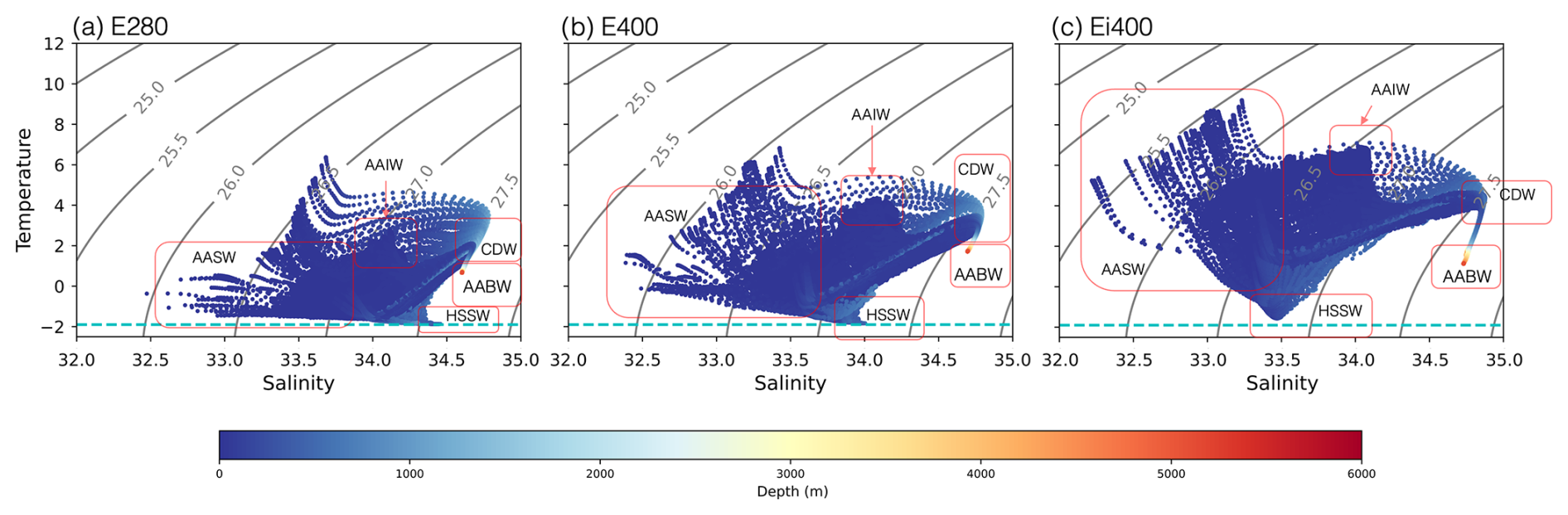
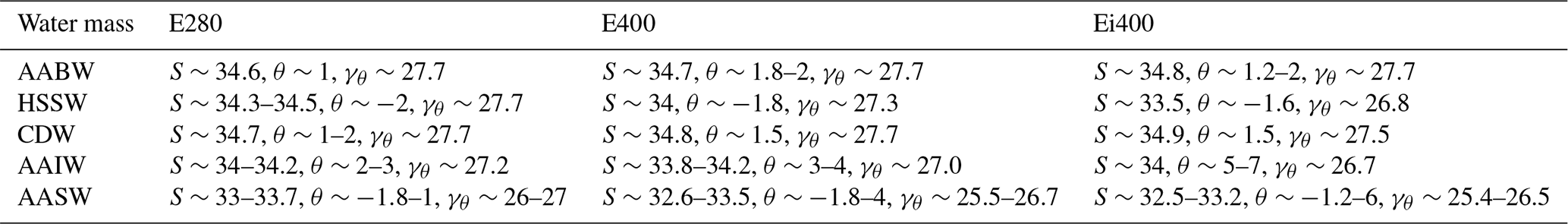
Figure 10 Potential temperature (θ)–salinity (T–S) diagrams of the Southern Ocean for (a) E280, (b) E400, and (c) Ei400, averaged over the last 200 simulation years. Grey solid lines show the isopycnals of 24.5–28 kg m⁻³. Note that the colour scheme refers to the depth at which water masses are formed in the Southern Ocean. The cyan dashed horizontal line shows the surface freezing point of seawater (1.8 °C). Major water masses are labelled as Antarctic Surface Water (AASW), Antarctic Intermediate Water (AAIW), Circumpolar Deep Water (CDW), High Salinity Shelf Water (HSSW), and Antarctic Bottom Water (AABW).

Table 3 Thermohaline properties and density location of Southern Ocean water masses highlighted in Fig. 10. Density is the potential density anomaly γ_θ (kg m⁻³) relative to 1000 kg m⁻³. The order of properties in the column representing the experiments is salinity (S; PSU), potential temperature (°C), and density (γ_θ).

Upon comparing E400 and Ei400 with E280, all water masses displayed in Fig. 10 are formed at warmer temperatures. This reflects the overall warming of the water column that is observed in Fig. 7b and d. Conversely, the evolution of salinity during runtime in Fig. 7a and c displays a contrasting pattern within the entire water column, which is also reflected in the overall lighter densities that are occupied by these water masses. Specifically, the AASW is the lightest water mass (${\mathit{\gamma }}_{\mathit{\theta }}<\mathrm{27}\mathrm{kg}{\mathrm{m}}^{-\mathrm{3}}$) displayed in Fig. 10, which loses buoyancy during winter through brine rejection and is transformed into the HSSW (${\mathit{\gamma }}_{\mathit{\theta }}>\mathrm{27}\mathrm{kg}{\mathrm{m}}^{-\mathrm{3}}$) and which subsequently descends through the water column and feeds the AABW. On the other hand, the CDW, brought through the Meridional Overturning Circulation (MOC), is an important water mass that, via diapycnal mixing with AASW and HSSW, directly contributes to AABW formation (Pardo et al., 2012). In E400 (Fig. 10b), the AABW is contracted, and the AASW and HSSW become substantially fresher and lighter, with respect to E280. This indicates a reduced dense shelf overflow that ultimately weakens the AABW formation. As CDW becomes saltier and warmer to a degree that does not modify its density and the upwelling induced by the westerlies is not increased during runtime, its entrainment into the Southern Ocean is not able to destabilise the stratification towards promoting more deep-water formation.

Conversely, in Ei400, the AABW is expanded, becoming denser and saltier, while maintaining its temperature in comparison to E280. Additionally, the change in thermohaline properties and the density of the AASW and HSSW are amplified with respect to E400, but the CDW becomes saltier, which suggests enhanced entrainment of saltier waters into the Antarctic shelf and a subsequent increase in abyssal salinity. These processes combined justify the partial recovery of the AABW towards the end of the Ei400 simulation, even with relatively stable conditions in the upper ocean. In summary, freshening of the upper ocean induces increased stratification in both experiments that reduces the export of dense shelf water to the bottom of the ocean and results in an overall AABW suppression in the first years of the E400 and Ei400 experiments. However, reducing the ice sheets imposes an extra freshening and warming of the upper ocean that further isolates the ocean interior, while the subsurface and deeper ocean undergo a more intense salinisation that occurs in increased AABW formation, not necessarily induced by the change in ice sheet itself but by possible teleconnections with other ocean basins further north.

4 Discussion

In E400, Antarctic warming is modest overall. Air temperature changes are most pronounced in areas experiencing sea ice loss and associated decline in surface albedo, such as the Weddell Sea. This surface warming flattens the meridional temperature gradient (Kidston et al., 2011), whilst the loss of sea ice further smooths the surface, suppressing storm development (Screen et al., 2011). This leads to weaker westerlies and a shift to a negative SAM phase (Fig. 3b), which aligns with studies showing a negative SAM in response to regional or seasonal reductions in Antarctic sea ice (Thompson et al., 2005; Marshall, 2003). The negative SAM contributes to stabilising the upper layer of the Southern Ocean (Fig. 7) via weaker westerlies that prevent interior mixing (Tamsitt et al., 2017) and the entrainment of cold, dense waters onto the Antarctic continental shelf. The more extensive sea ice loss in the Pacific in Ei400, together with weakened wind regimes throughout the APF, drives a contraction of the seasonal SIZ and reduces Antarctic divergence (Ramadhan et al., 2022), further suppressing the upwelling of warm CDW, which further leads to the cooling confined to the Pacific sector of the Southern Ocean. This behaviour is consistent with current observations (Beadling et al., 2022; Roach et al., 2023; Schmidt et al., 2023). With increased stratification at deep convection sites induced by freshening and warming of the upper ocean, together with the negative SAM phase, vertical mixing required for deep-water formation is limited, which occurs in the suppression of the AABW.

In Ei400, an intense pSH warming leads to complex and regionally varying atmospheric responses, agreeing with the consensus from the Pliocene Model Intercomparison Project (PlioMIP2) that the influence of a strongly reduced AIS exacerbates the changes induced by a higher CO₂ concentration alone. The strongest warming (up to 16 °C) is located over and inland from the Ross and Weddell seas, an area also showing the largest albedo declines (up to 50 %) and significant sea ice losses. The observed inland Antarctic warming pattern dominated by the Ross, Ronne, and Amery ice shelves is consistent with physical expectations, as these low-altitude, relatively warm ice shelves act as heat reservoirs, facilitating heat transfer inland. The magnitude of ocean and atmospheric warming displayed in our findings exceeds the magnitude suggested for the LP by the PlioMIP2 ensemble (Weiffenbach et al., 2024). However, these large atmospheric and sea surface temperature increases observed are likely influenced by the Southern Ocean bias prevalent in the EC-Earth3 (Döscher et al., 2022) model and by the large spread in the large-scale patterns of climate change simulated by the PlioMIP2 ensemble (Haywood et al., 2020). Such uncertainty in the PlioMIP2 ensemble is also a motivation for the development of the third phase of PlioMIP, PlioMIP3 (Haywood et al., 2024), and therefore does not jeopardise the quality of the findings displayed here or their significance to the scientific community.

We also observe adjacent zones of both wind and pressure strengthening and weakening, pointing to disrupted and complex wind regimes around Antarctica, particularly over the continent itself. These non-zonally symmetric changes in both wind and pressure patterns are consistent with the idea that regional feedbacks and non-linearities emerge once the ice sheet is reduced. An example is the weakening of the westerly winds over the Southern Ocean between 50–60° S. Such weakening aligns with the reduction in the Equator-to-pole temperature gradient, which weakens the zonal pressure gradient that drives the westerly jet. In Ei400, the tropical regions warm by 2.32 °C, but Antarctica warms by 9.18 °C, drastically reducing the meridional temperature contrast from 42.1 °C in the control to 37.3 °C. A weakening of the gradient leads to a weaker, more meandering jet and a less stable negative SAM pattern (Thompson and Wallace, 2000; Gerber and Vallis, 2007). This weakening of the westerlies also substantially impacts the advection of surface warmer waters by the ACC and leads to a decrease in the formation of coastal polynyas that contribute to sea ice formation and salinisation of the deeper layers of the Southern Ocean (Kusahara et al., 2017).

Regarding deep-water formation, under both elevated atmospheric CO₂ concentrations and LP ice sheet extent, water masses formed in the Southern Ocean experience major changes, especially related to AABW, AAIW, and CDW formation and export, agreeing with evidence for a weakening of Southern Ocean circulation during past warm geological periods (Noble et al., 2020). This has been noted in the Miocene (Herold et al., 2012), with reduced Southern Hemisphere westerlies weakening global overturning circulation and deep-water upwelling at the Antarctic divergence during the Late Pliocene, where a highly stratified Southern Ocean weakens the abyssal overturning circulation (Weiffenbach et al., 2024), and in the LIG, where Yeung et al. (2024) demonstrate a subdued ACC, primarily driven by weaker deep-ocean convection due to reduced sea ice formation leading to changes in meridional density gradients and surface winds. This reoccurrence throughout different palaeo-periods illustrates that there are numerous key and shared mechanisms responsible for driving changes in the Southern Ocean circulation, which are also displayed in our study.

Specifically with respect to AABW formation, the climatic consequences of the forcing induced through our sensitivity experiments affect sea ice formation and the development of stratification in the water column. The impacts of elevated CO₂ and LP ice sheet extent directly affect the formation processes of the AABW, a process that depends largely on sea ice dynamics and the interplay between salinity and temperature in the water column. Under pre-industrial climate conditions, the water column remains stable during summer through the balance between meltwater input from sea and land ice and the cold temperatures of the Southern Ocean, whereas the salinity increase induced by brine rejection during sea ice formation in winter induces the formation of cold, dense waters towards the ocean bottom layer (Silvano et al., 2023) and contribute to AABW formation. However, under enough climatic forcing, the AABW can be suppressed, and its variability can drastically change when comparing to PI conditions. A reduced AABW formation can arise from meltwater input in the Southern Ocean, such as from freshwater pulses from the retreating WAIS following the LIG, as modelled by Menviel et al. (2010), or freshwater discharge from the modern retreat of the AIS in the 21st century, as modelled by Gorte et al. (2023). Alternatively, surface buoyancy loss and stronger westerlies over the Southern Ocean can also inhibit AABW formation and export through induced upwelling of the CDW, thereby reducing dense shelf water formation that is a contributor to AABW. This was noted by Watson et al. (2015) to have occurred during the LGM, when upwelling was shifted further away from the Antarctic coast, resulting in the densest waters not being formed at the continental margin, prohibiting AABW formation. Conversely, weaker easterly winds can also reduce sea ice formation at deep convection sites and further inhibit AABW formation via increasing areas of open water, primed for air–sea buoyancy loss and convective overturning, demonstrated by Schmidt et al. (2023) to occur throughout the 20th century. On the other hand, disruption of subpolar westerly wind regimes may also indirectly boost AABW formation, through limiting the accumulation of freshwater around the Southern Ocean and aiding in the process of upper-ocean resalinisation after freshwater forcing has ceased (Trevena et al., 2008). Changes to AIS topography offer another mechanism by which deep-water formation in the Southern Ocean can be reduced, illustrated by the PlioMIP2 ensemble of experiments incorporating full boundary changes (Haywood et al., 2013). Under these idealised experiments, the lowered AIS elevation reduces the temperature gradient between Antarctica and surrounding air masses, weakening katabatic winds and affecting sea ice production towards restricting dense water formation. Altered AIS topography also impacts other aspects of atmospheric circulation, shifting the Southern Hemisphere westerlies poleward and leading to the aforementioned northward shift in upwelling. Thus, the dynamics that accompany cycles of AABW formation, either through suppression or strengthening, are highly complex and not linear through past warm or cold climates. This reinforces the need to continue to investigate deep-water formation in the Southern Ocean under various regimes, as we do here in our study. Ultimately, we show that the isolated effect of albedo-driven warming of the Southern Ocean and melting of sea ice hinders AABW formation and weakens the SMOC through inducing more stratification in the water column. Our findings therefore parallel the underlying mechanism, as exhibited by other studies, of enhanced upper-ocean stratification suppressing deep convection, without a freshwater forcing or topographic change. Thus, our study shows that reduced ice sheets not only amplify surface-driven feedbacks but also initiate deep-ocean processes that partially mitigate the suppression of deep-water formation, which in itself is a novel perspective, since our experiments on all these particularities have not been performed before.

5 Conclusions

There is a notable gap in existing research on the isolated impact of the abrupt removal of large portions of ice sheets on climate and ocean circulation. In this study, we specifically isolate the climatic response to ice sheet retreat to examine its role in driving Antarctic climate dynamics and Southern Ocean circulation, highlighting the Southern Ocean's critical sensitivity to increased atmospheric warming. We utilise the Late Pliocene as an important analogue of future climate scenarios due to its modern-like atmospheric CO₂ concentrations and significantly reduced ice sheets. This palaeogeographic framework offers a valuable opportunity to assess climate sensitivity to regional ice sheet extent changes.

Incorporating the glacial-isostatic-driven orographic changes that accompany ice sheet reduction in both hemispheres would undoubtedly increase the realism of our experiment, as, under future ice sheet loss, the resulting changes in orography are likely to have significant impacts on both the surrounding and global climate and oceans. A large reduction in AIS elevation may lead to strong local warming and a strengthening of poleward energy and momentum transport by baroclinic eddies, whilst the increasing outgoing longwave radiation from the localised warming may drive anomalous southward energy transport toward the continent, resulting in cooling elsewhere (Singh et al., 2016). Therefore, the atmospheric and oceanic responses observed in our sensitivity experiments with isolated PRISM4D ice sheet conditions do not fully reproduce the climate changes seen in more comprehensive modelling studies that incorporate all boundary conditions of the Late Pliocene, nor do they fully match the reconstructed climate based on proxy data (Burls et al., 2017; Haywood et al., 2013, 2016a, 2024). However, as our primary objective is to isolate the climatic response to ice sheet extent reduction, by holding orography fixed and focusing on idealised sensitivity experiments, we demonstrate that ice sheets play a critical role in modulating climate feedbacks in response to warming.

Reconstructing and applying Late Pliocene palaeogeography remains an important avenue for future experiments, and an extended set of sensitivity experiments would provide valuable insights into future climate change and even reduce existing model biases. These include a freshwater hosing experiment introducing a redistributed flux equivalent to the ice sheet volume that is reduced in the Late Pliocene relative to the pre-industrial, the implementation of the reconstructed orography changes intrinsic to the PlioMIP3 guidelines for the ice sheet sensitivity experiments to assess how orographic changes interact with albedo and freshwater forcing, experiments with various concentrations of imposed atmospheric CO₂ forcing, and the implementation of interactive ice sheets to capture the transient nature of ice–climate feedbacks.

By isolating the climatic response to ice sheet extent reduction, our study provides a foundational understanding of how ice sheet loss, independent of freshwater input and orographic changes, can significantly alter Southern Hemisphere climate dynamics. We have demonstrated, even under present trends, that the ability of the Southern Ocean to ventilate the deep ocean is at significant risk. These insights are critical for refining future climate models, offering a clearer picture of the potential pathways and risks associated with polar ice sheet instability.