the Creative Commons Attribution 4.0 License.
the Creative Commons Attribution 4.0 License.
 | 17 Oct 2025
A new biogeochemical modelling framework (FLaMe-v1.0) for lake methane emissions on the regional scale: development and application to the European domain
Manon Maisonnier
David Bastviken
Sandra Arndt
Ronny Lauerwald
Aidin Jabbari
Goulven Gildas Laruelle
Murray D. MacKay
Wim Thiery
Pierre Regnier
This study presents a new physical-biogeochemical modelling framework for simulating lake methane (CH4) emissions at regional scales. The new model, FLaMe-v1.0 (Fluxes of Lake Methane), rests on an innovative, computationally efficient lake clustering approach that enables the simulation of CH4 emissions across a large number of lakes. Building on the Canadian Small Lake Model (CSLM) that simulates the lake physics, we develop a suite of biogeochemical modules to simulate transient dynamics of organic Carbon (C), Oxygen (O2), and CH4. We first test the performance of FLaMe-v1.0 by analyzing physical and biogeochemical processes in two theoretical lakes with characteristics that can be considered representative for many lakes (an oligotrophic, deep lake driven by cold climate versus a eutrophic, shallow lake driven by warm climate). Next, we evaluate the model by comparing simulated and observed timeseries of CH4 emissions in four well-surveyed lakes. We then apply FLaMe-v1.0 at the European scale to evaluate simulated diffusive and ebullitive lake CH4 fluxes against in-situ measurements in both boreal and central European regions. Finally, we provide a first assessment of the spatio-temporal variability in CH4 emissions from European lakes with a surface area comprised between 0.1–1000 km2 (n= 108 407, total area = 1.33 × 10⁵ km2), indicating a total emission of 0.97 ± 0.23 Tg CH4 yr−1, with the uncertainty constrained by combining FLaMe-v1.0 and machine learning techniques. Moreover, 30 % and 70 % of these CH4 emissions are through diffusive and ebullitive pathways, respectively. Annually averaged CH4 emission rates per unit lake area during 2010–2016 have a South-to-North decreasing gradient, resulting in a mean over the European domain as 7.39 g CH4 m−2 yr−1. Our simulations reveal a strong seasonality (with ice-blocking effects accounted for) in European lake CH4 emissions, with nearly ten times higher emissions during late summer than during winter. This pronounced seasonal variation highlights the importance of accounting for the sub-annual variability in CH4 emissions to accurately constrain regional CH4 budgets. In the future, FLaMe-v1.0 could be embedded into Earth System Models to investigate the feedback between climate warming and global lake CH4 emissions.
- Article
(4570 KB) - Full-text XML
-
Supplement
(8502 KB) - BibTeX
- EndNote


Methane (CH4) is the second most important greenhouse gas after carbon dioxide (CO2), with a Global Warming Potential (GWP) per mass ∼ 28 times higher than that of CO2 over a 100-year horizon (Saunois et al., 2020). Over the last centuries, the atmospheric CH4 concentration has increased from 722 ppb in the pre-industrial period (year 1750) to 1923 ppb in year 2023 (Saunois et al., 2020; Lan et al., 2024; Forster et al., 2024) and this increase is expected to continue in the future. The critical role of CH4 in global warming has called for the establishment of a comprehensive global CH4 budget, which embraces both natural and anthropogenic sources (Saunois et al., 2016, 2020, 2025). This budget identified inland freshwaters (lakes, reservoirs, ponds, rivers, etc.) as an important, yet highly uncertain atmospheric CH4 source (Jackson et al., 2020, 2024; Saunois et al., 2020; Canadell et al., 2021). Global lake CH4 emissions, which has been estimated to account for ∼ 5 % to 20 % of total CH4 emissions (576 Tg CH4 yr−1), are the largest contributors to this inland water source (Jackson et al., 2020; Saunois et al., 2020). However, estimates of its magnitude vary depending on the assessment methods, with discrepancies of up to a factor of four (Saunois et al., 2020; DelSontro et al., 2018; Rosentreter et al., 2021; Bastviken et al., 2011; Deemer et al., 2016; Johnson et al., 2022; Holgerson and Raymond, 2016; Stavert et al., 2021). This variability in global estimates also manifests itself at the continental scale. For instance, estimates of European lake methane emissions range from 0.9 to 2.5 Tg CH4 yr−1 (Petrescu et al., 2021, 2023; Lauerwald et al., 2023).
Observation-based upscaling approaches are highly dependent on the availability and quality of in-situ measurements, which are unevenly distributed across the globe and biased towards summer months (Canadell et al., 2021; Johnson et al., 2022). Although the number of CH4 emission measurements from lakes has increased considerably in recent decades, the two largest current databases together contain only 1081 records from 575 lakes worldwide (Rosentreter et al., 2021; Johnson et al., 2022). This relatively small data compilation is unlikely to capture the full diversity of physical and biogeochemical patterns of > 1.4 million lakes worldwide, which vary by morphology, climate, trophic status, and underlying sediment characteristics (Rinta et al., 2017; Bastviken et al., 2004; Bastviken, 2022; Deemer and Holgerson, 2021; Johnson et al., 2022). Even more critically, the underlying data collection was not designed to capture the inter-annual and decadal variability in CH4 emissions driven by climate change and nutrient dynamics, hence rendering the decomposition of the total lake CH4 fluxes into natural and human-induced components challenging (Saunois et al., 2020). Finally, although current instruments and techniques can effectively capture CH4 fluxes through diffusive (driven by gradients of aqueous CH4 concentrations) and ebullitive (via gas bubbles in the sediments due to oversaturation) emission pathways, measurements related to lake turnover events (release of previously accumulated CH4 due to stratification and ice cover) and transport through vegetation aerenchyma remain highly challenging (Denfeld et al., 2018; Mayr et al., 2020; Zimmermann et al., 2019). These limitations induce large uncertainties in observation-based upscaling methods. In this context, process-based modelling approaches – that rely on detailed representations of lake physical and biogeochemical processes informed and tested with the available observational data – offer complementary strategies to help reduce these uncertainties.
Process-based biogeochemical models provide powerful tools to upscale scarce observations, both in space and in time. In combination with the available observational datasets, they can help deliver regional and global estimates of lake CH4 emissions from daily to decadal timescales, as well as future projections. These mechanistic models can also help identify the drivers such as climate, land-use and atmospheric composition changes responsible for the complex temporal dynamics of lake CH4 emissions. Over the last decades, several process-based models have thus emerged, e.g., LAKE 2.0 (Stepanenko et al., 2016), bLake4Me (Tan et al., 2015), and ALBM (Tan et al., 2017; 2024), to estimate lake CH4 emissions to the atmosphere. These models explicitly account for the physical and biogeochemical processes that govern lake CH4 dynamics and resulting emissions. For instance, using ALBM, Zhuang et al. (2023) recently estimated that global lakes (larger than 0.1 km2) emit 24.0 ± 8.4 Tg CH4 yr−1, which is at the lower end of the range reported by Saunois et al. (2020) and represents 11 % of total global CH4 emissions from natural sources as estimated from atmospheric inversions. Yet, these process-based models also have limitations that need to be addressed. A central limitation is the omission of lake phytoplankton productivity, which is one of the most reactive organic C sources and thus substrates for CH4 production. In most of existing models, this key process and the associated microbial degradation of organic C is not simulated explicitly but taken as prescribed model inputs. If phytoplankton productivity and associated contributions of methane substrates can be incorporated in lake CH4 models, this would allow capturing the impacts of environmental conditions beyond the commonly included direct temperature effects on organic matter decomposition and CH4 production. Such additional important impacts include feedback of C metabolism on lake oxygen (O2) cycling along with eutrophication effects on CH4 emissions (DelSontro et al., 2018; Rosentreter et al., 2021; Stavert et al., 2021). However, it is challenging to explicitly describe the suite of key physical and biogeochemical processes controlling the coupled C-O2-CH4 cycles while at the same time maintaining model complexity, as well as the needs for observational data and computational costs for regional and global scale applications with tractable bounds. In addition, it also requires the quantification of nutrient inputs from the surrounding catchments, which exert a key control on lake productivity.
To tackle these challenges, we here develop a new process-based model framework of intermediate complexity, FLaMe-v1.0 (Fluxes of Lake Methane version 1.0,) that couples the C-O2-CH4 cycles in lakes using a one-dimensional representation. Specifically, FLaMe-v1.0 builds upon the existing physical lake model CSLM (Canadian Small Lake Model–MacKay, 2012; MacKay et al., 2017), and extends with a novel biogeochemical module that captures the production, oxidation, storage, transport and emissions of CH4 in/from lakes. Importantly, FLaMe-v1.0 introduces lake primary production and turnover of autochthonous organic carbon as a major driver of lake O2 and CH4 dynamics. The coupled, mechanistic lake model is then embedded in a computationally efficient clustering approach that allows for the application of the new, coupled, mechanistic lake model for (i) large parameter/input ensemble runs on regional/global scales for uncertainty assessments, (ii) long-term model projections for the assessment of future climate change and its feedback on the Earth system, (iii) a potential coupling to Earth System Models (ESMs) in subsequent stages of its development.
The structure of this paper is described as follows. In Sect. 2, we provide a general description of the lake model with a focus on a detailed description of the novel biogeochemical modules, as well as the parameter choices and numerical solutions. In Sect. 3, we first test the overall behavior of FLaMe-v1.0 using two theoretical, representative lakes (an oligotrophic, deep lake driven by cold climate versus a trophic, shallow lake driven by warm climate), and then evaluate the simulated temporal variations of CH4 fluxes against observational data at four well-surveyed lakes in the real world. Next, we apply FLaMe-v1.0 at the European scale and evaluate the results against in-situ measurements in boreal and central European lakes compiled by Rinta et al. (2017). Finally, we provide a spatio-temporally resolved estimate of CH4 emissions from European lakes (2010–2016), assess their sensitivity to key model parameters, and constrain their uncertainty range using a machine-learning approach. In Sect. 4, we discuss model limitations and potential directions for further research. Main conclusions and outlooks are drawn in Sect. 5.
2.1 General model approach
We developed a new process-based physical-biogeochemical model, FLaMe-v1.0 (Fluxes of Lake Methane), to simulate lake CH4 production and emission at large spatial scales. FLaMe-v1.0 resolves the interplay of physical and biogeochemical processes that governs organic matter (COC,auto), oxygen (O2), and methane (CH4) dynamics to estimate (diffusive and ebullitive) lake CH4 emissions, as well as CH4 storage fluxes due to lake turnover and ice melting. To enable a continental-scale application of FLaMe-v1.0 (e.g., in Europe, n= 108 407 and total area = 1.33 × 10⁵ km2 for lakes with 0.1 1000 km2 according to Messager et al., 2016; A0 is the lake surface area), we here propose a lake clustering strategy to reduce the computational and data/input costs (Fig. 1) while resolving the variability in lake sizes, morphology, and trophic status as well as climate conditions across Europe. Within each grid cell (2.5° × 2.5°), lakes are binned into four classes according to surface area (0.1–1, 1–10, 10–100, 100–1000 km2). We then run a FLaMe-v1.0 simulation for one representative lake per size class within each grid cell, using the arithmetic means of lake area, depth and trophic status of all lakes pertaining to the respective size class across the respective grid cell. Note that the areas and depths of all lakes are available from HydroLAKES database (Messager et al., 2016) while trophic status is derived from outputs of the GlobalNEWS model (Mayorga et al., 2010; Lauerwald et al., 2019). The total emission flux from a given size class can be obtained by multiplying the CH4 emission rates simulated by FLaMe-v1.0 with the total lake area of this size class (Fig. 1).
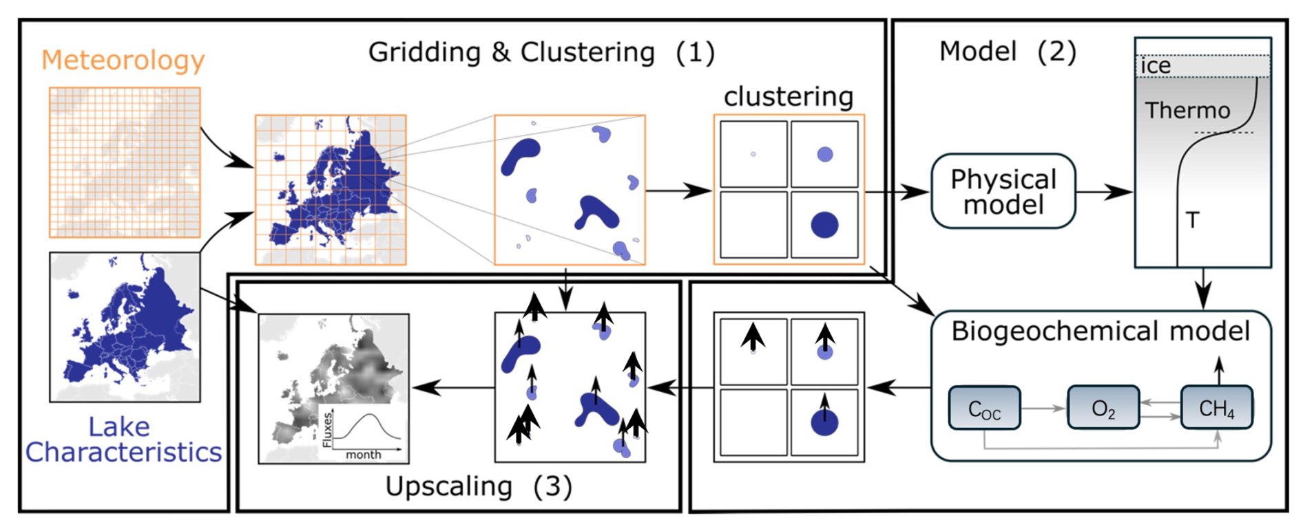
Figure 1Illustration of the lake clustering and upscaling strategy for the continental application of FLaMe-v1.0 (Europe as an example). (1) Gridding and clustering: The European domain was divided into grid cells at a coarse spatial resolution of 2.5° × 2.5°. Within each grid cell, lakes are clustered into four classes according to their surface areas. (2) FLaMe-v1.0 parallelization: FLaMe-v1.0 simulates the lake metabolic dynamics, vertically resolved concentration and rate profiles of the coupled O2-CH4 cycle as well as diffusive and ebullitive CH4 fluxes through the water-air interface. The model was parallelized under transient conditions for each grid cell and each lake class. (3) Upscaling: The areal rates (i.e., fluxes per unit lake surface area) simulated by FLaMe-v1.0 were then multiplied by the total surface area of each lake class within each grid cell (available from HydroLAKES) and aggregated at the monthly timescale. The arrows pertaining to clustered and original lakes represent the CH4 emissions and the arrow size represent the magnitude of the flux (i.e., a lower flux for larger lakes).
2.2 Model description
FLaMe-v1.0 builds on an online coupling approach between the Canadian Small Lake Model (CSLM; MacKay, 2012; MacKay et al., 2017) – a widely used lake physics model (Garnaud et al., 2022; Verseghy and MacKay, 2017; William et al., 2014) – and a set of newly developed biogeochemical modules that resolve lake OC, O2 and CH4 dynamics. We selected the CSLM as the basis of the representation of lake physical processes in FLaMe-v1.0 because CSLM was designed for small lakes that accounts for > 90 % of lakes (by number, mean depth < 7.8 m) but contribute disproportionally to lake CH4 emissions in the European domain (HydroLAKES; Messager et al., 2016), as well as due to the expertise in our research team. CSLM simulates the following physical variables: temperature profile (T), thermocline depth (hmix, at which the vertical temperature gradient reaches its maximum), photic depth (hphot, down to which the sunlight can penetrate, with radiation density of at least 1 % of that at the lake surface), and ice cover, which will be used to force the biogeochemical modules (Fig. 2). In turn, the biogeochemical module will later modify the photic depth simulated by CSLM to account for the effect of phytoplankton growth and self-shading on light penetration, thus resolving the feedback between lake biogeochemical processes and lake physical dynamics, hence forming a complete feedback loop. A detailed description of the well-established CSLM model can be found in MacKay (2012) and MacKay et al. (2017) and is also briefly presented in Sect. S1 in the Supplement. Compared with other lake models (Table S1), the most important improvements in FLaMe-v1.0 are the adoption of a “valley” shape lake set up and the incorporation of autochthonous carbon dynamics (i.e., explicit simulation of primary production, decomposition, and oxygen processes) and its phosphorus limitation, which have been shown to be key control factors of CH4 dynamics (Søndergaard et al., 2017; Guildford and Heckay, 2000; Schindler, 1977). In what follows, we provide a detailed description of the vertically resolved 1D model set-up (Sect. 2.2.1) used here, as well as of the novel biogeochemical modules (Sect. 2.2.2). All the involved model parameters, their values, and ranges are summarized in Table 1 (Sect. 2.3).
Table 1Model parameters of FLaMe v1.0 and the choice of their values.
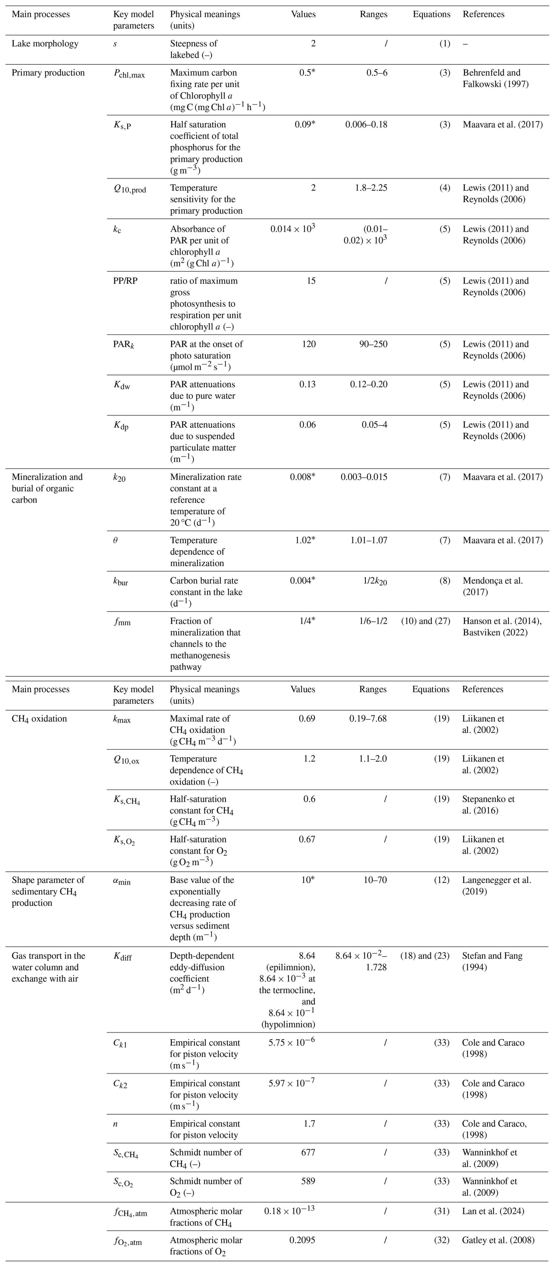
* indicates that the original parameter values are from the literature, and further adjusted by calibration versus observations. Moreover, their values are varied for the sensitivity analysis in Sect. 3.3.3. / indicates that the ranges of the parameter values are not reported.
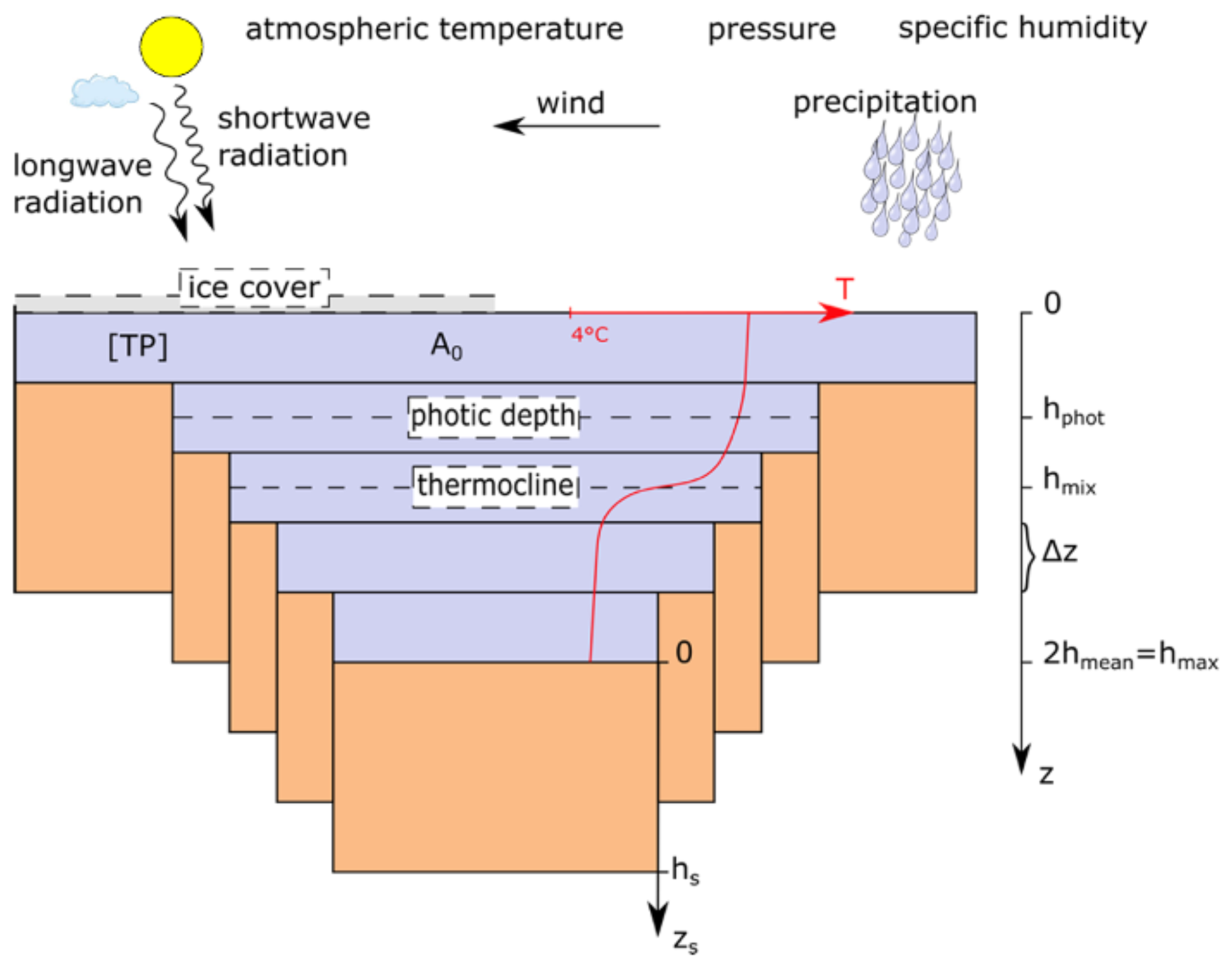
Figure 2Schematic representation of the lake morphology in FLaMe-v1.0. The lake is represented by a “valley” shape (denoted by Eq. 1). A0 denotes the lake surface area, A is the area of each water layer, and hmax is the maximal water column depth. z represents the depth of a water column down to the surface of a sediment column while zs stands for the depth inside a sediment column (zs= 0 at the sediment-water interface). The physical model is forced by longwave and shortwave radiations, near-surface wind, precipitation, atmospheric temperature, pressure, and specific humidity. Purple color indicates the water layers, and orange color indicates the sediment columns.
2.2.1 Model Scope: Idealized representation of lake morphology
Figure 2 illustrates the vertically resolved, one-dimensional model set-up of FLaMe-v1.0 that is used for both the physical and biogeochemical modules. The original version of CSLM usually adopts a “bucket” shaped morphology which assumes a constant area (A) versus water depth (z), i.e., A(z)= A0, where A0 is the lake surface area at z= 0 m. However, this morphology is unsuitable for the simulation of biogeochemical processes, especially when variations in water depth within each lake are important. Therefore, we, instead, adopted a “valley” shaped lake morphology, with lake area A(z) given by:
where A is the lake area (m2), z is the water depth (m), s is a shape parameter that controls the slope of the lakebed (a larger s indicates a steeper slope), and hmax is the maximum lake depth. To ensure that the volume (and hence heat exchange) is conserved between the “bucket” and “valley” shape set-ups, the maximum depth of the valley-shape lake, hmax, must be twice that of the mean depth of the bucket-shape lake, hmean (i.e., hmax= 2hmean), which was extracted from the global HydroLAKES database compiled by Messager et al. (2016). The bottom temperature profiles simulated by CSLM were then extended to the maximal depth of the valley shape lake.
Physical processes in the water column are simulated by CSLM, on a one-dimensional, vertically resolved, evenly distributed grid with a grid spacing of 50 cm. Each layer of the water column is connected to a vertically integrated lake sediment column of 5 m depth (hs, m) (Langenegger et al., 2019) (Fig. 2). Since the CH4 production rate decreases exponentially with sediment depth (not applicable to thermokarst lakes), it is typically negligible at 5 m within the sediment column (Langenegger et al., 2019), thus ensuring that the total, depth-integrated benthic CH4 production becomes insensitive to this arbitrary choice. The surface area of each sediment column in contact with the water column is determined by difference in the widths of two adjacent water layers A(z) (Eq. 1). In addition, it should be noted that we assume no horizontal material exchanges (O2 and CH4) between the sediments and water columns (i.e., across the interface where left and right edges of a water layer touch the sediment box; Fig. 2) because of its relatively minor magnitude compared to the vertical exchanges (Stepanenko et al., 2016; Tan et al., 2024) as well as the lack of observational data. Therefore, only the vertical exchanges are simulated in this first version of the model (see details in the following sections).
2.2.2 Biogeochemical Modules
Organic carbon module
Following the approach of Maavara et al. (2017), FLaMe-v1.0 does not resolve the vertical distribution of labile (i.e., microbial degradable) organic carbon (OC) concentrations ([COC,auto]) produced by in-lake primary production, but only simulates the temporal dynamics of the volume-integrated autochthonous OC stock (, g C) (the overbar here indicates a volume-integrated value). should be understood as a simple indicator or an overall reflection of the resulting lake trophic status, itself controlled by the combined effects of climate and nutrient loads from the catchment. The allochthonous C inputs delivered from surrounding catchments are more refractory and generally have a slower decomposition rate (Grasset et al., 2018; Guillemette et al., 2017; DelSontro et al., 2018), although CH4 production from allochthonous OC has in some instances been reported to be higher than from autochthonous compounds in laboratory incubations (Grasset et al., 2018). Thus, we consider the allochthonous OC as less important substrates for CH4 production, and consider the autochthonous primary production as the only labile OC source in this first model version; the allochthonous OC contribution will be added in the future upgrade of the model.
The temporal evolution of volume-integrated labile OC stock is determined by the interplay between autochthonous primary production, pelagic and benthic mineralization and burial fluxes (Maavara et al., 2017):
where t is time (day), and is the volume-integrated OC stock (g C). , and are the volume-integrated primary production, mineralization, and sedimentary burial fluxes (g C d−1), respectively. Following Maavara et al. (2017), we assume that autochthonous primary production rates are controlled by the light regime, water temperature, and the lake total phosphorus (TP) concentration ([TP], g P m−3) (Reynolds, 2006). The volume-integrated can then be expressed using a classical Michaelis-Menten formulation (Maavara et al., 2017):
where B is the phytoplankton biomass (expressed as chlorophyll a concentration, g Chl a m−3) in the photic zone (Eq. 5), PChl,max is the maximum carbon fixation rate per unit of chlorophyll a (g C (g Chl a)−1 h−1), M is a dimensionless metabolic correction factor that depends on the mean lake water temperature in photic zone Tmean (°C) (see Eq. 4), Ks,P is the half-saturation constant for phosphorus limitation (g P m−3), and Vphot is the water volume above the photic depth (m3). Parameters PChl,max and Ks,P are constrained based on published observations (see Sect. 2.3), while the metabolic factor M is given by:
where Q10,prod is the temperature sensitivity for primary production, quantifying the increases of the metabolic factor per 10° increase in temperature. Surface water phytoplankton biomass, B, is approximated by a function of the photosynthetically active radiation (PAR), which is determined by shortwave radiation and light extinction in the water column:
where kc is the absorbance of PAR per unit of chlorophyll a (m2 (g Chl a)−1), and is the ratio of maximum gross photosynthesis to respiration per unit chlorophyll a. PAR0 is the PAR at the lake surface (µmol m−2 s−1), determined by the incoming shortwave radiation, as well as the daytime that is specified by lake latitude and phenology (represented by the day of the year). PARk is the PAR at the onset of photosaturation (µmol m−2 s−1). The productive depth hprod is determined as the maximum of the thermocline and the photic depth simulated by the physical model. Kdw, Kdp, and Kdg represent nonalgal PAR attenuations, due to pure water, inorganic suspended particulate matter, and labile carbon, respectively. Following Lewis (2011), Kdg is calculated as a function of [COC,auto] as:
Equation (5) was derived based on the assumption of a balance between production and respiration (Reynolds, 2006; Lewis, 2011). Here we slightly relax this assumption and assume near-equilibrium conditions for given climate conditions at the monthly timescale, allowing us to simulate seasonal variations of primary production and associated biogeochemical processes. Note that this assumption is only used for biogeochemical variables related to primary production, while physical variables simulated by CSLM are resolved at a sub-daily time step.
Following Hanson et al. (2011, 2014) and Maavara et al. (2019), the volume-integrated mineralization rate is simulated as a function of temperature and labile OC availability:
where k20 is a first-order rate constant for the mineralization of at 20 °C (d−1). Tmean is the mean water temperature (°C) in photic zone, and θ is the temperature dependence of mineralization of organic matter (Hanson et al., 2014).
Following Maavara et al. (2019), the burial flux is represented by a first order process driven by the labile OC stock :
where kbur is the burial rate constant and here set as half of the mineralization rate constant following the ratios between these two processes reported in the global lake dataset (n= 230) assembled by Mendonça et al. (2017). This ratio is likely an upper bound because it accounts for contributions of both autochthonous and allochthonous carbon sources in the dataset, while allochthonous inputs should have higher burial/decomposition ratios than autochthonous ones (Mendonça et al., 2017; Guillemette et al., 2017).
Methane module
The methane module simulates the dynamics of CH4 concentration in both sediment and water columns as controlled by CH4 production, aerobic CH4 oxidation, and diffusive and ebullitive transport from sediment to water and atmosphere (Fig. 3). Since the observational evidence suggests that benthic CH4 production is the dominant CH4 source in lakes (Tan et al., 2015; Bastviken, 2022), we neglect the CH4 production within the lake's water column in the model.
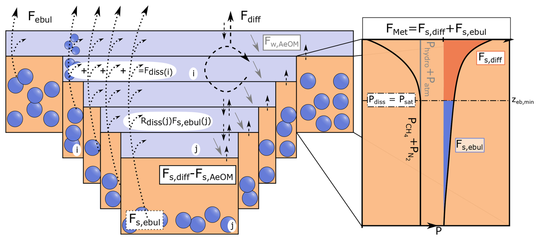
Figure 3Illustration of the methane (CH4) module of FLaMe-v1.0 with a zoom into benthic CH4 dynamics (zoom modified from Langenegger et al., 2019). Benthic CH4 production (zoom) assumes an exponential decrease in CH4 production rate (FMet) with depth. The CH4 and N2 partial pressures ( ) is mainly driven by the CH4 production and follows the black curve profile, which starts to exceed the sum of the hydrostatic and atmospheric pressure (Phydro+ Patm − , grey line) at zeb,min. Thus, this depth (zeb,min) divides FMet into a diffusive (Fs,diff, red filled region) and an ebullitive (Fs,ebul, cyan filled region) flux. Fs,AeOM and Fw,AeOM are the CH4 oxidation in the sediment and water column, respectively. Fdiss is the dissolution of the gas bubbles during transport through the water column. Fdiff and Febul are diffusive and ebullitive CH4 fluxes through the water-air interface, respectively. i and j are the indexes of water layers and sediment columns. Note that the sediment column pertaining to a particular water layer has the same index as that water layer.
Within the lake sediment, CH4 dynamics are determined by the balance between CH4 production via methanogenesis and CH4 migration to the water column through diffusive and ebullitive transport:
where the tilde overbar here represents the volume-integrated stocks or fluxes in the sediment column, which is different from the straight overbar for volume-integrated values in the water column. Note that we have sediment columns at different water depths, such that the stocks and fluxes are represented as a function of water depth z, which is characterized by the valley-shape model set-up and different from the conventional bucket shape set-up. is thus the volume-integrated CH4 stock for the sediment column with the sediment-water interface positioned at depth z (g CH4). is the volume-integrated flux of CH4 production through the entire sediment column with a sediment-water interface at depth z (g CH4 d−1), and and are volume-integrated diffusive and ebullition fluxes (g CH4 d−1) through the sediment-water interface at depth z, respectively. fmm denotes the fraction of organic matter mineralization that proceeds via methanogenesis according to data compiled by Hanson et al. (2014) and Bastviken (2022). M is a conversion factor corresponding to the molar ratio of CH4 to COC,auto. As is the total CH4 production flux integrated over the whole water column, we assume that the fractions of CH4 production occurring in different sediment columns are set according to their volume proportions, i.e., .
The partitioning of CH4 production into ebullitive and diffusive fluxes depends on the porewater CH4 concentration or its partial pressure, which relies mainly on the vertical distribution of CH4 production rate in the sediment as well as the oxygen concentration (but is of second-order importance). Based on the observation-based assumption that the organic carbon concentration and thus mineralization rates exponentially decrease with sediment depth, we here assume an exponentially decreasing relationship between methanogenesis rate versus depth (Fig. 3), following Langenegger et al. (2019):
where fmet(z,zs) is the methanogenesis rate (g CH4 m−3 d−1) at sediment depth zs for the sediment column with the sediment-water interface positioned at depth z. FMet,0(z) is the maximum CH4 production at the sediment-water interface (g CH4 m−3 d−1) at depth z, and α is a shape parameter (m−1) that controls the decrease of methanogenesis rate with depth. As the shape of this curve typically depends on the flux of labile carbon settling on the lake bottom, and thus, lake trophic status, the parameter α is here scaled by the FPP empirically:
where αmin is the minimum or base value, and β is the dependence of α on FPP. The values of αmin and β are determined based on the measurements in lakes of different trophic status reported by Langenegger et al. (2019).
To determine the maximum CH4 production FMet,0(z), the integral of CH4 production rate over sediment column should equal to the volume-integrated CH4 production flux as specified by Eq. (10):
where As(z) is the surface area of sediment column in contact with the water layer at lake depth z and is determined by difference in the areas of two adjacent water layers A(z) (Eq. 1). The maximum CH4 production at depth z, FMet,0(z), can be obtained by combining Eqs. (10), (11) and (13):
Since CH4 production increases the in-situ CH4 concentration as the sediment depth increases, the CH4 concentration may exceed its solubility concentration and methane gas bubbles may start forming (Fig. 3). To constrain the partitioning of CH4 production between diffusion and ebullition, the threshold sediment depth, zeb,min, at which CH4 concentration starts to exceed the solubility limit, is determined based on the equilibrium pressure condition following Langenegger et al. (2019) (see details in Sect. S2). In the upper portion of the sediment column (zs < zeb,min), the produced CH4 will diffuse into water; however, a fraction of the diffusing CH4 will be oxidized in the transit through the upper sediment column, and only the remaining CH4 will reach the sediment-water interface. The volume-integrated CH4 oxidation in the sediment at depth z, , is here assumed to be controlled by the O2 concentration in the overlying bottom water, and is represented by a Michaelis-Menten function:
where is the half-saturation constant of O2 for the sedimentary CH4 oxidation. As a result, the diffusive flux passing through the sediment-water interface is determined as follows:
In the lower portion of the sediment column (zs > zeb,min; where oversaturation occurs), the produced CH4 feeds the ebullitive flux, with the volume-integrated value (g CH4 d−1) as given by:
Note that Eqs. (16) and (17) implicitly imply that, at the monthly resolution of our model, the CH4 dynamics in the sediment is at steady state and all the CH4 produced during this time interval is either oxidized or released through the water column via diffusive and ebullitive pathways.
Pelagic, dissolved CH4 diffuses in the water column and its concentration is determined by the diffusive CH4 flux passing through the sediment-water interface (acting as a source for each water layer), by aerobic CH4 oxidation in the water column, and by the re-dissolution of the ebullitive CH4 fluxes during transit through the water column. The mass conservation equation of dissolved CH4 is then given by:
where [CH4]w is the pelagic CH4 concentration (g CH4 m−3) and Kdiff is the eddy diffusion coefficient of CH4 in water (m2 d−1). is the change of CH4 concentration induced by diffusive inputs from the sediment columns, the term A(z)dz being the volume of the water layer connected to the corresponding sediment column. Fw,AeOM(z) is the aerobic CH4 oxidation rate in the water column, and is described through double Michaelis-Menten reaction kinetics (Stepanenko et al., 2016; Liikanen et al., 2002; Thottathil et al., 2019):
where kmax is the maximum CH4 oxidation rate (Liikanen et al., 2002), T is the water temperature, Tr is the reference temperature, and Q10,ox expresses the temperature dependency of the CH4 oxidation rate. and are the half-saturation constants for CH4 and O2, respectively.
To constrain the redissolution of gas bubbles (Fdiss(z)), we follow the approach proposed by McGinnis et al. (2006) where a function (fbdiss(z)) is used to represent the fraction of the benthic ebullitive CH4 flux that redissolves in the water column during gas ascent. This fraction is a function of water depth and gas bubble diameter, and the latter was set to 5 mm following Delwiche and Hemond (2017). With this function fbdiss(z), the redissolved CH4 fluxes from sediment column at depth z are assumed to be evenly redistributed in the water layers above the sediment, i.e.,
where is the water volume above the sediment layer at the depth of interest z. Then, at this particular depth z, the redissolution flux (Fdiss, g CH4 m−3d−1) is thus determined as follows:
where represents the integral of all re-dissolved ebullitive fluxes from sediment columns below z.
By deducing this dissolution flux from the ebullitive flux released from lake sediments, the resultant ebullitive flux reaching the atmosphere (Febul; g CH4 m−2 d−1) is calculated as:
where A0 is the lake surface area, and is the component of ebullitive flux at depth z that reaches the atmosphere.
In addition to diffusive and ebullitive pathways, FLaMe-v1.0 also calculates a storage flux (Fstor) that encapsulates the changes in the total CH4 mass stored in hypolimnion due to the weakening of lake stratification or turnover events when the lake surface temperature approaches the critical temperature 4 °C (MacKay, 2012; MacKay et al., 2017). This results in a full mixing of the lake that releases the previously accumulated CH4 in the anoxic portion of the lake and concomitantly fully aerates the water column. Lake turnovers thus lead to a complete homogenization of O2 and CH4 concentration across the vertically resolved water column. Before lake turnover, the lake water is highly stratified, blocking the material exchange between upper and lower water layers, such that bottom water has high CH4 concentration (even oversaturated) and low O2, while the upper water has high O2 concentration and low CH4 concentration. Upon full mixing, remobilization of larger CH4 stocks that accumulated in the hypolimnion abruptly increase the CH4 concentration near the lake surface, and hence strongly enhance the diffusive flux through the air-water interface; in the meantime, O2 in the upper layers can penetrate to deep water layers and start oxidizing the CH4 throughout the entire water column. After full mixing, the CH4 emissions and oxidation are both simulated based on O2 and CH4 concentrations within each water layers. That is, the storage flux in FLaMe-v1.0 is not simulated separately but it is implicitly incorporated into the diffusive flux Fdiff which increases dramatically following the formation of a very sharp CH4 concentration gradient at the lake surface.
Oxygen module
The oxygen module is needed to simulate the lake methane processes (see Methane module). It represents the O2 cycle within the water column, driven by O2 production by photosynthesis, O2 consumption by pelagic and benthic OC mineralization, and aerobic pelagic and benthic CH4 oxidation. These processes are coupled to the vertical diffusive transport of O2 through water column (Fig. 4). The one-dimensional conservation equation for O2 concentration in the water column is thus given by:
where [O2] is the O2 concentration in the water (g O2 m−3), and Kdiff is the eddy diffusion coefficient of O2 (m2 d−1), assumed identical to that of CH4. OFPP(z) is the oxygen production through primary production (g O2 m−3 d−1) at depth z. OFw,Aer(z) is the O2 consumption by heterotrophic respiration (g O2 m−3 d−1) in the water column at depth z, while is the volume-integrated O2 consumption by heterotrophic respiration in the sediment (g O2 m−3 d−1), and A(z)dz is the volume of the water layer connected to the corresponding sediment column. OFw,AeOM(z) and OFs,AeOM(z) are the aerobic CH4 oxidation in the water column and sediment (g O2 m−3 d−1), respectively, at depth z.
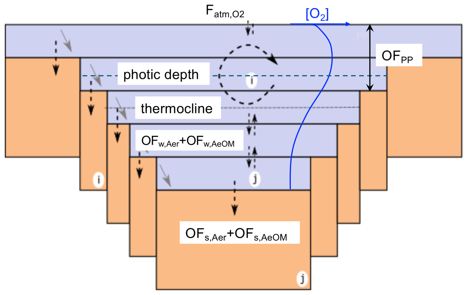
Figure 4Illustration of the oxygen (O2) module in the FLaMe-v1.0. The O2 production due to primary production occurs only in the photic zone (OFPP), while the O2 consumption by heterotrophic respiration occurs in both the entire pelagic zone and benthic zone (OFw,Aer and OFs,Aer). The O2 consumption due to CH4 oxidation occurs also in both pelagic and benthic zones (OFw,AeOM and OFs,AeOM). Fatm,O2 is the O2 exchange flux between water and atmosphere. In this figure, the dotted arrows crossing the sediment-water interface represent the O2 demands in sediments (OFs,Aer and OFs,AeOM), the dashed arrows represent the eddy diffusion of O2 between water layers and through the water-air interface, and the tilted grey arrows represent the aerobic oxidation of CH4 in the water column. As a result, the blue curve depicts a typical vertical profile of O2 concentration under lake water stratification.
Photosynthesis occurs only in the photic zone, and the amount of O2 produced by primary production (volume-integrated value; g O2 d−1) can be determined according to the stoichiometric ratio , where and MC are the molar masses of oxygen and carbon, respectively. To resolve the vertical O2 profile, the O2 produced during primary production is assumed to be evenly redistributed within the water layers above the photic depth (Fig. 4):
where Vphot is the photic volume.
The oxygen consumption induced by CH4 oxidation in the sediment and water column can be calculated from corresponding CH4 fluxes, Eqs. (15) and (19), respectively, and the stoichiometry of the reactions involved:
As in Eq. (10), a fraction of the mineralized organic carbon (represented by fmm) is channeled into the methanogenesis pathway according to the data compiled by Hanson et al. (2014) and Bastviken (2022). Thus, the remaining fraction (1–fmm) of the total mineralization is channeled into the aerobic metabolic pathway (FAer). As a result, the bulk volumetric rate of oxygen consumption due to the aerobic metabolic activity (OFAer) can be represented by the fraction 1−fmm and the volume-integrated mineralization :
In the sediment, the aerobic mineralization occurs only in the upper oxic layer. The thickness of this aerobic layer is limited by the oxygen penetration depth zox. Following Ruardij and Van Raaphorst (1995), this depth zox can be derived by solving the steady-state reaction-diffusion equation for O2 in the sediment:
where Ks,diff is the molecular diffusion coefficient within the sediment, which is dependent on the temperature (Ruardij and Van Raaphorst, 1995). The amount of O2 consumed within the oxic layers of the sediment can thus be determined as:
where As(z) is the area of the corresponding sediment column at depth z. To ensure a mass balance, the volumetric rate of O2 consumption due to aerobic metabolism in water can then be calculated as follows:
where A(z)dz is the volume of the water layer connected to the corresponding sediment column, and it is used here to convert the sedimentary O2 consumption into a volumetric rate in the water column. Furthermore, following Martin et al. (1987), Carlson et al. (1994) and Arístegui et al. (2003), we redistribute the respiration (OFw,Aer) within the water column, assuming that 80 % of the respiration occurs in the photic zone, with the remaining 20 %, sustained by the export production, occurs in the deeper water layers where it can further degrade.
2.2.3 Boundary conditions for the transport module
The partial differential Eqs. (18) and (23) require boundary conditions to constrain the diffusive transport (i.e., the first term on the right-hand side of both equations). At the sediment-water interface, a zero-flux boundary condition is imposed, because the diffusive exchanges of CH4 and O2 between the sediment columns and the overlying waters are already included as source/sink terms in Eqs. (18) and (23). This choice was guided by the valley-shape configuration of our lake set-up, and thus by the presence of diffusive CH4 and O2 exchange fluxes with sediment in each water layer of our model, a situation in stark contrast from a bucket shape model where only a single sediment column would be connected to the bottom water layer.
At the lake surface (z= 0 m), the boundary conditions are determined by the CH4 and O2 exchange fluxes with the atmosphere, as given by Wanninkhof et al. (2009) and Cole and Caraco (1998):
where and are diffusive fluxes of CH4 (g CH4 m−2 d−1) and O2 (g O2 m−2 d−1) through the air-water interface of the lake, respectively. and are molar fractions of CH4 and O2 in the atmosphere, respectively, and Patm is the atmospheric pressure. and are Henry's constants of CH4 and O2 at 298.15 K and kge is the piston velocity (m s−1), here constrained from the empirical equation reported by Cole and Caraco (1998), as in Tan et al. (2015, 2017) and Stepanenko et al. (2016):
where Ck1, Ck2 and n are empirical constants (Cole and Caraco, 1998). va,10 is the absolute wind velocity measured at 10 m above the lake surface (m s−1), and and are the Schmidt number of CH4 and O2, respectively (Wanninkhof et al., 2009). Note that more recent formulations of kge have been published in the last decade (Wanninkhof, 2014; MacIntyre et al., 2021) but we here choose to use Eq. (33) to be consistent with previous lake modelling studies (Tan et al., 2015; Stepanenko et al. 2016; Tan et al., 2017).
2.3 Parameter values
Table 1 summarizes all physical and biogeochemical parameters, their values, as well as the original references from which they were extracted. Most of these parameters were either directly taken from relevant modelling studies or constrained based on comprehensive literature reviews. In addition, several key parameters of the FLaMe-v1.0, highlighted in Table 1, were adjusted by calibrating the model based on observations of lake C fluxes (i.e., FPP, diffusive and ebullitive CH4 emissions). For instance, the parameters PChl,max and Ks,P control the lake primary production and were tuned to reproduce broad global patterns of primary production rates across the full range of lake trophic status (Wetzel, 2001). The mineralization k20 and burial constants kbur were adjusted based on the observed fraction of COC,auto that settles onto the lake sediment, either to be decomposed in anoxic or oxic conditions or accumulated in the sediment (Hanson et al., 2011, 2014; Maavara et al., 2019; Mendonça et al., 2017). The temperature dependence of mineralization θ was fine-tuned to reproduce the observational ranges of temperature dependence of net-CH4 emissions (Aben et al., 2017). fmm specifies the fraction of mineralization that channels to the methanogenesis pathway, which is adjusted to produce the observational patterns of CH4 emissions. αmin is the base value of the exponentially decreasing rate of CH4 production versus sediment depth, and controls the split of CH4 production between diffusive and ebullitive pathways, which was calibrated to reproduce observed broad trends of Ftot, Febul and Fdiff from the literature (Rinta et al., 2017). The parameter values listed in Table 1 provide the reference setup for the simulation of lake CH4 emissions, and the sensitivity and uncertainty analyses regarding the key model parameters (indicated by asterisks in Table 1) is carried out using wide ranges of values covering most possible lake conditions from the real world (see Sect. 3.3.3).
2.4 Numerical solution
In FLaMe-v1.0, the physical (i.e., CSLM) and biogeochemical (OC, CH4 and O2) modules are coupled online. For the dynamics of volume-integrated OC and CH4 in sediments, the involved ordinary differential equations are solved using a forward Euler scheme. For the dynamics of dissolved O2 and CH4 concentrations in the water column, the partial differential Eqs. (18) and (23) are solved numerically using an explicit central difference scheme for depth and Euler forward scheme for time. The diffusion coefficient Kdiff for both O2 and CH4 is set as depth-dependent (Table 1) to capture the reduced transport when the temperature gradient from the epilimnion, metalimnion and hypolimnion is well pronounced (Dong et al., 2020; Imboden and Wüest, 1995; Imberger, 1985; Boehrer and Schultze, 2008).
2.5 Case studies
We implemented three case studies to assess the performance of FLaMe-v1.0 in simulating lake CH4 emissions, as well as its application to the European scale. First, we present theoretical simulations for two representative cases (methodological details in Sect. 2.5.1) to assess the general behaviors of FLaMe-v1.0 in capturing the physical-biogeochemical patterns of contrasted lakes. Then, we perform the simulations for four well-surveyed real lakes to assess the model's capability in capturing the observed temporal variations of CH4 fluxes (Sect. 2.5.2). Next, we apply FLaMe-v1.0 to the entire European domain to assess the model's capability in reproducing the spatial patterns and seasonal variations of CH4 fluxes at continental scale (Sect. 2.5.3). The European scale application can be considered as a “proof of concept” in support of our proposed modeling strategy. Finally, we examine the sensitivity to key model parameters and assess the uncertainty of the continental-scale emissions using the samples produced by sensitivity analysis, combined with a machine learning approach (Sect. 2.5.4).
2.5.1 Two theoretical representative lakes for testing FLaMe-v1.0 performance
To test if the FLaMe-v1.0 can capture the contrast patterns in physical-biogeochemical behaviors across shallow vs. deep, eutrophic vs. oligotrophic and warm vs. cold lakes, we set-up the model for two theoretical representative lakes: a “deep oligotrophic” lake (hmax = 35 m or hmean= 17.5 m and [TP] = 3 µgP L−1) driven by a “cold” climate (63.75° N, 26.25° E; Fig. S1) and a “shallow eutrophic” lake (hmax= 10 m or hmean= 5 m and [TP] = 80 µgP L−1) driven by a “warm” climate (43.75° N, −6.25° E; Fig. S2). The lake areas of these two theoretical lakes were set as 5 km2, which was tested to have limited effects on the simulation results. For these two theoretical representative cases, FLaMe-v1.0 simulates the spatio-temporal evolutions of physical and biogeochemical variables and fluxes, including primary production and mineralization fluxes, and labile autochthonous OC stocks as well as the vertically resolved gradients of temperature, CH4 and O2 concentrations. Furthermore, we also compared the seasonal patterns of CH4 productions and emissions for these two contrasting lakes. To investigate further how environmental factors affect the model behavior, we further decompose the collective responses of shallow and deep lakes into individual effects induced by trophic level, climate (Figs. S1–S3) and lake depth using hypothetical numerical simulations, i.e., (i) changing the maximal lake depth (hmax) from 5 to 25 m; (ii) increasing the [TP] levels from 8 to 80 µgP L−1; and (iii) changing the climate from warm (43.75° N, −6.25° E; Fig. S1) to cold conditions (63.75° N, 26.25° E; Fig. S2).
2.5.2 Simulations of temporal patterns for four well-surveyed lakes
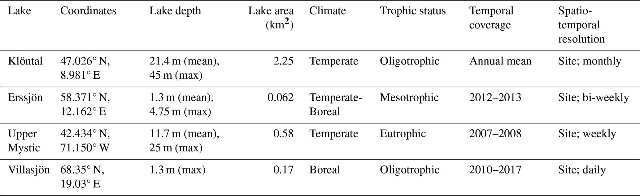
To evaluate the ability of FLaMe-v1.0 to reproduce the observed temporal patterns of CH4 fluxes, we selected four lakes from the Inter-Sectoral Impact Model Intercomparison Project (ISIMIP) lake datasets for which monthly resolved temporal CH4 fluxes were available (Tan et al., 2024). These lakes cover different lake depths, areas, climate conditions and trophic statuses, as summarized in Table 2. Since in-situ measurements of climatic drivers are not available for these lakes, we extracted them from the 0.5° × 0.5° GSWP3-W5E5 global climate forcings released by the ISIMIP3a project as an approximation. The measurements of CH4 fluxes for these lakes were mostly collected during the first 20 years of the 21st century, and we thus selected the climate forcings for the period 1991–2019, using the period 1991–1999 as spin-up phase. Since the lack of concomitant in-situ measurements of climatic drivers and variations in lake water levels affect the model's ability to capture the full variability in the time-series of observed CH4 emission time series, we here focus our evaluation on the magnitudes and broad seasonal patterns in observed CH4 emissions, following what can be achieved for regional and global scale applications. Thus, we evaluated the simulated statistics (mean and SD represented by boxplots) of CH4 fluxes over the annual cycle against the observational data.
Table 2Characteristic information for the four well-surveyed lakes from ISIMIP datasets.
2.5.3 Implementation of FLaMe-v1.0 at continental scale
To implement the model at the scale of Europe (25° W–60° E, 36–71° N), we extracted the natural lakes (type I) within this domain from the HydroLAKES database (Messager et al., 2016; n= 108 407, total area = 1.33 × 10⁵ km2 for lakes with 0.1 1000 km2 within the European domain). Following our clustering strategy, we subdivided, within each grid cell, all lakes into four classes based on their surface area (0.1 < A0 < 1 km2, 10 km2, km2, and 1000 km2). As FLaMe-v1.0 was derived from the small lake physics model CSLM, we here only considered the lakes with an area smaller than 1000 km2, and excluded the very large lakes (A0 > 1000 km2) that account for 40 % of the total European lake surface area (but only consist of 21 lakes). Within our model domain, we have 108 407 lakes with a surface area larger than 0.1 km2, which at spatial resolution of 2.5° (Figs. S4–S5) result in 365 grid cells and 953 representative lakes (hence reducing computation cost by more than a factor of 100 compared to a case where each individual lake would be simulated). By parallelizing the model simulations on a high-performance cluster, the implementation of FLaMe-v1.0 for the entire European domain consumes approximately 365 CPU hours for a single run covering 10 years.
The FLaMe-v1.0 was forced by meteorological conditions from the GSWP3-W5E5 reanalysis product under ISIMIP3a (Frieler et al., 2024) (Fig. S6), including shortwave solar radiation (W m−2), longwave solar radiation (W m−2), precipitation (mm s−1), near surface air temperature (at 10 m height, °C), specific humidity (kg kg−1), near surface wind velocity (at 10 m, m s−1), and atmospheric pressure (Pa). As these forcings were provided at a finer spatial resolution of 0.5°, we only applied the values in the central 0.5° grid cell of our larger 2.5° grid. In addition, the FLaMe-v1.0 was also driven by the TP in the representative lakes (Figs. S7–S8), which was estimated by dividing the TP mass outflow by the water discharge reported in HydroLAKES, hence assuming that the lake water is well mixed. The TP mass outflow from each lake in HydroLAKES was obtained by routing the TP loads (extracted from the GlobalNEWS model; Mayorga et al., 2010) from the watershed (point and non-point terrestrial sources) into the river network, following the procedure outlined in Lauerwald et al. (2019) and topological information provided by the HydroSHEDS drainage network. More details related to the TP routing can be found in Bouwman et al. (2009), Van Drecht et al. (2009), and Mayorga et al. (2010).
To validate the FLaMe-v1.0 for European lakes, we will evaluate the simulated FPP and CH4 emission rates against the ranges/values reported in the literature and/or from observations. First, the simulated FPP will be evaluated against empirical ranges reported by Wetzel, (2001) for lakes from ultraoligotrophic (0–5 µgP L−1), oligotrophic (5–10 µgP L−1), mesotrophic (10–30 µgP L−1), to eutrophic (> 30 µgP L−1) conditions. Next, the simulated diffusive and ebullitive CH4 emission rates will be evaluated against in-situ measurements compiled by Rinta et al. (2017) from 17 boreal lakes (in southern Finland and Sweden) and 30 central European lakes (in The Netherlands, Germany and Switzerland). This dataset is adopted because it can not only differentiate the ebullitive and diffusive CH4 fluxes during late summer (August and September, 2010–2011) but also provides information regarding environmental conditions of the study area (mean annual air temperature, annual precipitation, percentage of forests and managed land in the catchment) and water chemistry of the studied lakes (temperature, conductivity, pH, absorbance, TP and TN in surface water, and average TP and TN in the water column), which are helpful for understanding the lake methane dynamics within these two contrasted regions. However, this dataset of 47 lakes still has some important limitations, in particular as it presents only summer-time observations, and not time-series which would comprise the full seasonal cycle including turnover events and other hot moments. In addition, it contains potential biases induced by the calculation methods used for separating the measured CH4 fluxes into diffusive and ebullitive pathways. In particular, Rinta et al. (2017) used floating chambers over a relatively short duration (6 h), which might not be able to detect sporadic ebullition events, and did not employ bubble traps to estimate the ebullitive flux.
2.5.4 Sensitivity and uncertainty analysis
To explore how model parameterization affects the European-scale assessments of lake CH4 emissions, we conducted a sensitivity analysis encompassing the parameters whose variations induce the largest changes in lake CH4 dynamics (with the involved parameters indicated by asterisks in Table 1). The sensitivity was conducted by varying a parameter once at a time: only one parameter is varied with the other parameters kept unchanged. All these parameters were assumed to have Gaussian distributions, with their SDs specified as 50 % of their original values, except the temperature dependency Q10,ox and θ whose SDs were specified as 50 % of their deviation to unity. More specifically, we tested the sensitivity within the ranges of mean ± SD at four points, i.e., +SD, +0.5 SD, −0.5 SD, and −SD.
To constrain uncertainties in European scale CH4 emissions, we complemented the sensitivity analysis (n= 36) with another 28 scenarios under several extreme cases and different combinations of variations in key parameters. With these 64 assessments taken as samples, we then used a machine learning approach to assess the uncertainty associated with our estimation of European lake CH4 fluxes. Specifically, we trained a Random Forest (RF) model that capture nonlinear relationships between our key model parameters and European lake CH4 emissions, i.e., the key parameters are taken as predictors and the European lake CH4 emissions are taken as target variable. Next, we produced 1000 Gaussian-distributed random samples within the parameter space and estimated an ensemble of CH4 emissions using the trained RF model.
3.1 Assessing the performance of FLaMe-v1.0 in capturing patterns of CH4 dynamics across different lake types
The FLaMe-v1.0 is shown to be able to well capture the typically observed, contrasting physical and biogeochemical behaviors for two representative cases (Figs. 5 and S9–17; more details in Sect. S3): shallow vs. deep, eutrophic vs. oligotrophic and warm vs. cold lakes. In the deep oligotrophic lake, the mean temperature reveals a lower and narrower seasonal variability (∼ 3–8 °C) compared to the shallow eutrophic lake (5–15 °C) (Fig. 5a vs. b). Large temperature variations in the latter are mainly driven by the smaller water volume and thus faster mean temperature response to fluctuations in atmospheric temperature. In addition, the annual averaged FPP in the shallow eutrophic lake (490 gC m−2 yr−1) is approximately 38 times higher than that in the deep oligotrophic lake (13 gC m−2 yr−1) (Fig. 5c vs. d). This difference can be explained by the differences in water volume (energy exchange), trophic status, and climate forcings. The higher FPP of the shallow eutrophic lake also translates into higher COC,auto concentration (∼ 110 times) which persist over longer periods (Fig. 5e vs. f), despite substantially higher Fmin rates.
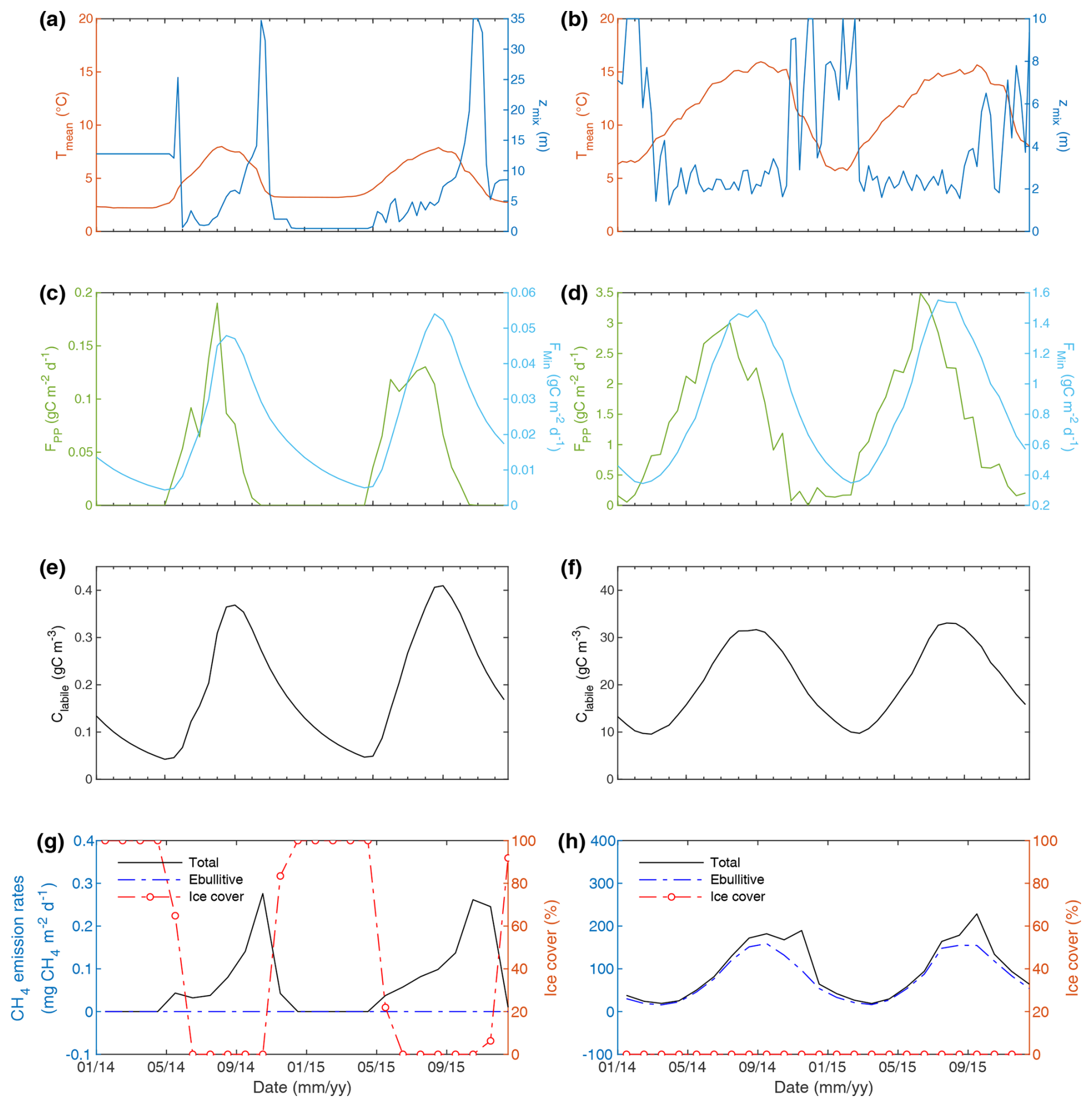
Figure 5Depth-integrated temporal evolution of variables and processes in two theoretical representative lakes. The deep oligotrophic lake (left) has a maximal depth of 35 m and [TP] of 3 µgP L−1, and is driven by the climate forcings at the location of 63.75° N, 26.25° E. The shallow eutrophic lake (right) has a maximal depth of 10 m and [TP] of 80 µgP L−1, and is driven by the climate forcings at the location 43.75° N, −6.25° E. (a) and (b) show the evolution of lake mean temperature and mixing depth; (c) and (d) show the evolution of primary production (FPP) and mineralization rate (FMin); (e) and (f) show the evolution of concentration of autochthonous organic carbon (COC,auto); (g) and (h) show the evolution of CH4 emission rates and ice cover. Note the different scales between the left and right panels.
In the deep oligotrophic lake, the simulated vertical temperature profiles indicate an almost permanently maintained stratification that is only interrupted by short but intense turnover events during late falls (Fig. S9a). Lake stratification (e.g., lake turnover and O2 concentrations that depend mostly on solubility and hence, temperature) dominates the spatio-temporal pattern of O2 such that O2 concentration is near-saturated during most of the year (Fig. S9c). The oligotrophic status, together with the well oxygenated conditions, results in extremely low CH4 concentrations. Higher CH4 concentrations are only simulated near the lake bottom following the productive season, i.e., late summer/fall transition (Fig. S9e). In contrast, in the shallow eutrophic lake, the weaker stratification results in a less pronounced vertical temperature gradient (Fig. S9b). The vertical lake O2 profile is not only controlled by the lake physics (temperature and O2 solubility) but also by intense biogeochemical processes (Fig. S9d). During summer, O2 concentrations in the upper portion of the lake are slightly supersaturated due to photosynthetic activity, followed by a gradual decrease in O2 concentration as mineralization rates exceed primary production rates. Due to the high primary production in the eutrophic lake, large amounts of OC are exported below the thermocline, where heterotrophic activity progressively depletes O2, leading to the development of anoxic conditions in the hypolimnion. The combination of high FMin and low O2 concentrations drive the accumulation of CH4 in late summer at the bottom of the lake (Fig. S9f), with maximal CH4 concentration (3.0 g CH4 m−3) exceeding those simulated in the deep oligotrophic lake by a factor of 600 (Fig. S9e).
By aggregating CH4 fluxes over time, we obtained distinct seasonal patterns of CH4 production and emission for these two representative lakes (Figs. 5g, h and S10). In the cold, deep oligotrophic lake (Figs. 5g and S10a), winter to early spring ice cover (December–April) blocks CH4 emissions such that lake CH4 emissions are limited to the period between May and November. CH4 production is highest (0.8 mg CH4 m−2 d−1) in August and lowest (0.08 mg CH4 m−2 d−1) in April. Almost all the produced CH4 escapes the sediment via diffusion as gas bubbles do not form due to low CH4 production rates and high-water pressure. However, the benthic CH4 flux is subsequently largely oxidized in the well oxygenated deep water column. As a result, total lake CH4 emissions are low (0 to 0.24 mg CH4 m−2 d−1) with a slight peak in October. In the shallow eutrophic lake (Figs. 5h and S10b), the warmer climate prevents ice formation on the lake surface, leading to an emission season about twice as long as under colder climatic conditions. CH4 production (20 to 350 mg CH4 m−2 d−1) is > 1000 times higher than that in cold, deep oligotrophic lake due to the higher nutrient loads, lower O2 levels, higher irradiance as well as higher temperature (Fig. 5b). Higher CH4 production rates, together with lower water pressure, drive the formation of gas bubbles, leading to a higher fraction of CH4 emissions via the ebullitive pathway. The weaker stratification and the shorter transport time scale in the shallow lake limits CH4 oxidation during diffusive transport, leading to ∼ 900 times higher total CH4 emissions compared to the deep, oligotrophic lake. Total lake CH4 emissions are highest (210 mg CH4 m−2 d−1) in September and lowest (20 mg CH4 m−2 d−1) in February.
By decomposing the collective responses of shallow and deep lakes into individual effects induced by trophic level, climate and lake depth using additional theoretical numerical simulations, we found that the trophic level exerts the most important control on CH4 dynamics, followed by climate, and finally, lake depth (Figs. S11–S14). Specifically, the yearly mean CH4 production is increased by a factor of 30 (from 3 to 89 mg CH4 m−2 d−1), and the yearly mean CH4 emission is increased by a factor of 44 (from 1.3 to 57 mg CH4 m−2 d−1) from oligotrophic to eutrophic status (i.e., [TP] increased by 10 times) (Fig. S12). From cold to warm climate, the yearly mean CH4 production and emission increase by a factor of 6 (9.4 to 59 mg CH4 m−2 d−1) (Fig. S13), and a factor of 5 (5.7 to 30 g CH4 m−2 d−1), respectively. By increasing lake depth from 15 to 35 m (Fig. S14), the CH4 production rates remain almost the same, i.e., 20 mg CH4 m−2 d−1 for the yearly mean and 60 mg CH4 m−2 d−1 for the peak, while the CH4 emissions are overall lower (35 to 22 mg CH4 m−2 d−1 for the peak without considering the storage flux) for the deeper lake.
3.2 Evaluation of simulated temporal lake CH4 emissions against observations from four well-surveyed lakes
In Klöntal and Erssjön Lakes (Table 2, Fig. 6a and b), FLaMe-v1.0 captures the observed seasonal cycles of CH4 emissions well, albeit with almost a one-month delay. As a result, the simulated CH4 fluxes are slightly lower in the first half of the year and slightly higher in the second half. This lag between observations and model results is likely due to the use of idealized climate forcings but could also be attributed to the unresolved changes in water levels and in-lake TP dynamics. In the Klöntal Lake (Fig. 6a), the observed CH4 fluxes are exceptionally high in April (1.64 mg CH4 m−2 d−1) and July (5.03 mg CH4 m−2 d−1), interrupting the normal seasonal cycles. These abrupt observed emissions might reflect the contributions from storage fluxes that are not well captured by FLaMe-v1.0. Apart from these two months with exceptionally high fluxes, the observational data indicates peak emissions of 3.18 mg CH4 m−2 d−1 in August and no emissions during the ice-covered period. FLaMe-v1.0 simulates similar fluxes, with a peak of 3.4 mg CH4 m−2 d−1 in September (and 3.17 mg CH4 m−2 d−1 in August), and a null flux in January–February when the model predicts ice formation. In the Erssjön Lake (Fig. 6b), observational data report a peak in CH4 emission reaching 13.48 mg CH4 m−2 d−1 in July and no emissions during the ice-covered period, whereas FLaMe-v1.0 simulates a peak emission of 18.76 mg CH4 m−2 d−1 in August (and 12.82 mg CH4 m−2 d−1 in July), and no flux in February. Moreover, the simulated CH4 fluxes are exceptionally high in April (11.10 mg CH4 m−2 d−1) due to the release of a storage fluxes that does not seem to be recorded by the observations. These high CH4 fluxes attributed to storage and lake turnover are usually associated with large variability, i.e., in Klöntal Lake (Fig. 6a), the observed variability (standard deviation, SD) in CH4 flux in July is almost 8-fold larger than the simulated one, whereas in Erssjön Lake (Fig. 6b), the simulated SD in CH4 flux in April is almost 6-fold larger than that of the observed one. This suggests that both in-situ measurements and FLaMe-v1.0 struggle to accurately capture the storage fluxes. Apart from these storage fluxes, we found that the SDs of CH4 fluxes simulated by FLaMe-v1.0 are lower than those observed for most months, indicating a more stable behavior in the simulations compared to the observations across the multi-year period considered here.
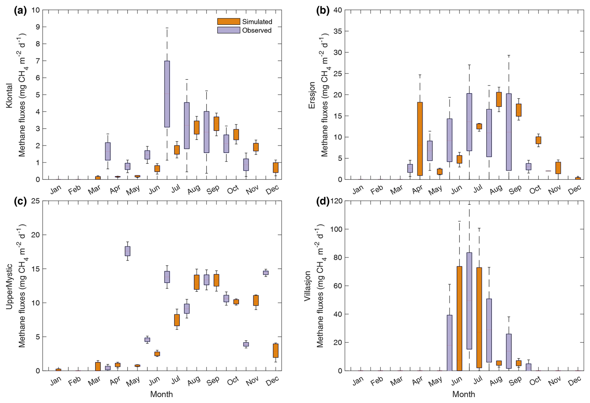
Figure 6Evaluation of FLaMe-v1.0 against monthly mean CH4 fluxes recorded in long time-series of observations in four real lakes. (a) Klöntal, (b) Erssjön, (c) Upper Mystic, and (d) Villasjön. The detailed lake characteristics are listed in Table 2. The climate forcings for these four lakes are extracted from GSWP3-W5E5 model from ISIMIP3a. Note the different scales of CH4 emissions in each lake.
For the Upper Mystic and Villasjön Lakes (Fig. 6c and d), the observed temporal patterns of CH4 fluxes appear more erratic, either due to the dominant role of short-term water level fluctuations or due to the complex ice cover dynamics. For the Upper Mystic Lake (Fig. 6c), the observed CH4 fluxes are irregular or fluctuating (0–17.6 mg CH4 m−2 d−1) over the year, a pattern which was explained by dynamic variations of lake water levels (Varadharajan, 2009). Since in-situ water level measurements are lacking and the lake area and depth are set as constant in the model, the simulated temporal variations cannot capture these observed erratic patterns well. Our model produces a smoother seasonal cycle of monthly-mean CH4 fluxes over the year, i.e., high fluxes (10.02–13.38 mg CH4 m−2 d−1) during the productive season (August–October), and low fluxes (0.02–7.56 mg CH4 m−2 d−1) during the other months. Moreover, the model predicts a weak storage flux occurring in November (10.20 mg CH4 m−2 d−1). For the Villasjön Lake (Fig. 6d), the observed CH4 fluxes are limited to the period of June–October, due to the long ice cover period induced by the cold climate. FLaMe-v1.0 captures the observed ice-cover period well and produces similar seasonal cycles of CH4 fluxes. The simulated means and SDs are very close to observations in June and July, but both, means and SDs, are much lower than observations in August, September, and October.
In summary, despite the use of idealized climatic forcing and neglecting variations in lake area and water level, FLaMe-v1.0 broadly captures the observed temporal patterns of monthly mean emissions, albeit sometimes with small delays or diverging extents of high emissions periods. The SDs of simulated CH4 fluxes are also usually lower than the observed values, which is to be expected considering that our model is not designed to capture high-frequency fluctuations of CH4 fluxes. The largest biases can be found in the estimations of storage fluxes (timing and magnitude), probably due to (1) the difficulty of capturing these fluxes with existing measurement instruments and techniques, (2) the possibility of methane oxidation with greater than expected values during turnover and ice-out (Mayr et al., 2020; Zimmermann et al., 2019; Pajala et al., 2023) and (3) the lack of in-situ measurements of climate conditions, dynamical water levels, and dynamic TP concentrations (Denfeld et al., 2018). Resolving these issues will require to assemble a much larger dataset of observed long time-series of CH4 fluxes and associated physical and biogeochemical variables, such as those reported by Rodríguez-Velasco et al. (2024) and Natchimuthu et al. (2017). To help further calibrate and evaluate the model, this much larger pool of observations should span a broader range of environmental conditions to be more representative of the lake CH4 dynamics on the continental to global scales. Overall, given the scarce spatiotemporal observations and the limited possibility to validate current knowledge on process regulation in fields, it is difficult for all existing models to produce the details of the CH4 dynamics in specific single lakes. Hence, the temporal patterns of CH4 fluxes simulated by FLaMe-v1.0 are seen as acceptable, as its main focus is to capture the broad spatio-temporal patterns of CH4 emissions across the thousands of lakes that need to be accounted for in large-scale applications (see Sect. 3.3).
3.3 FLaMe-v1.0 application on the European domain
3.3.1 Evaluation of FLaMe-v1.0 in European lakes
In the European scale application of FLaMe-v1.0, we first evaluated the simulated FPP against the empirical ranges reported by Wetzel (2001) for lakes under ultraoligotrophic (0–5 µgP L−1), oligotrophic (5–10 µgP L−1), mesotrophic (10–30 µgP L−1), and eutrophic (> 30 µgP L−1) conditions (Figs. 7 and S18). Figure 7 shows that, under different trophic status, the means and medians of FPP simulated by FLaMe-v1.0 (for 953 representative lakes) fall well within the reported ranges. Slight deviations could only be observed in ultraoligotrophic lake for which the model tends to slightly overestimate FPP (Fig. 7a). Ultraoligotrophic and oligotrophic lakes reveal very similar mean and median of FPP that fall at the higher ends of the ranges specified by Wetzel (2001) or even exceed it in the case of ultraoligotrophic lakes. In turn, mesotrophic and eutrophic lakes reveal mean and median FPP that fall at the lower ends of the ranges specified by Wetzel (2001). This slight difference of simulated versus observed FPP in lakes with different trophic conditions can be explained by the relatively low value of Ks,P (90 µg L−1) compared to the concentration of [TP] (Figs. S7–S8), as well as the simplified representation of lake primary production in our model. When extending the representative lakes to all real lakes in the European domain (n= 108 407), the median and mean of simulated FPP are still within the specified ranges but are reduced slightly for all trophic status (Fig. S18), attributed to the positively skewed distribution of [TP] (Fig. S8), i.e., many lakes have a low [TP].
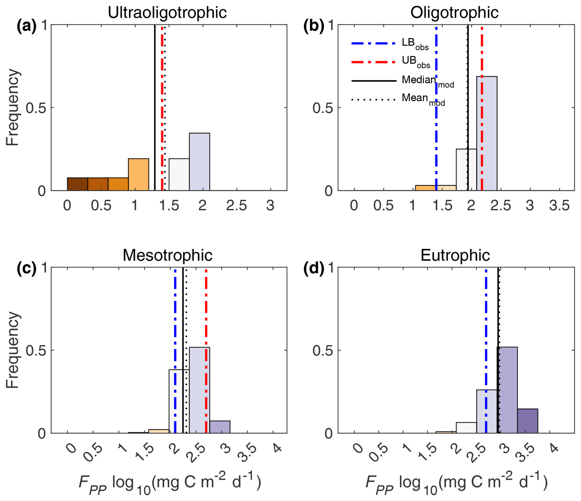
Figure 7Comparison of simulated primary production (FPP) with empirical estimates reported by Wetzel (2001). The histograms show the frequency distributions of simulated FPP (log scale) for 953 representative lakes that are grouped into ultraoligotrophic (0–5 µgP L−1), oligotrophic (5–10 µgP L−1), mesotrophic (10–30 µgP L−1), and eutrophic (> 30 µgP L−1) lakes. In the figure, blue and red dashed lines are the lower and upper bounds (LBobs and UBobs), respectively, of empirical ranges reported by Wetzel (2001) in this class of lakes; Black solid and dotted lines are the medianmod and meanmod, respectively, of simulated FPP for this class of lakes.
Next, we evaluated the simulated diffusive and ebullitive CH4 emission rates against measurements in boreal and central European regions during late summer (August–September, 2010–2011) synthesized by Rinta et al. (2017) (Figs. 8 and S19). As Rinta et al. (2017) compiled in-situ measurements of diffusive and ebullitive CH4 emission rates from 17 boreal lakes (in southern Finland and Sweden) and 30 lakes of central European lakes (in The Netherlands, Germany and Switzerland), we extracted the mean CH4 emission rates during August–September for representative lakes located in the grid cells corresponding to these two regions. Results indicate that the simulated diffusive CH4 emissions for boreal European lakes (Fig. 8) agree well with the observations; yet the simulated ebullitive CH4 emissions are slightly higher than the observations, leading to slightly higher total emissions. For central European lakes, the simulated diffusive CH4 emissions are slightly lower than the observations, while the simulated ebullitive CH4 emissions are slightly higher, leading to a good agreement in the total emissions (Fig. 8). The slightly higher ebullitive fluxes simulated by FLaMe-v1.0 may be attributed to not only the uncertain choice of model parameters (e.g., α) but also to the systematically lower measured ebullitive fluxes in Rinta et al. (2017), where ebullition was separated from diffusion when the measured fluxes produced unreasonably high k600. Moreover, Rinta et al. (2017) reported 6 and 27 times higher diffusive and ebullitive fluxes in central Europe, respectively, while our model simulates a smaller contrast of a 3- and 7-fold difference. This smaller contrast in the simulation can likely be explained by the higher variability in measurements, reflecting diverse climate, light and catchment properties in real lakes, while the variabilities in the simulated fluxes are significantly lower, probably due to more homogeneous representations of environmental conditions in the simulations. Specifically, the large differences in measured CH4 emissions in boreal and central European lakes are attributed to their distinct characteristics, including climate (colder and dryer in the boreal region), light regime (larger absorbance in the boreal region) and catchment properties, in particular land-use (dominance of forests and smaller fraction of managed agricultural land in the boreal region). However, in FLaMe-v1.0, the catchment properties are not fully captured by our sole, simplified indicator of [TP], such that the differences between boreal and central European lakes are underestimated. The coarse resolution of our model also likely reduces the represented range of climate conditions in our simulations compared to those experienced by the sampled lakes. In the meantime, observations are also associated with uncertainties, because measurements were not continuous in time and might thus not be fully representative of the late summer-early fall period, as well as sampling and measuring CH4 emissions, in particular via the ebullitive pathway, is all but a trivial task. Nevertheless, the above evaluation of FLaMe-v1.0 against observations overall reveals the ability of our model to reproduce broadly observed patterns in primary production and CH4 emissions observed across distinct trophic status and landscapes.
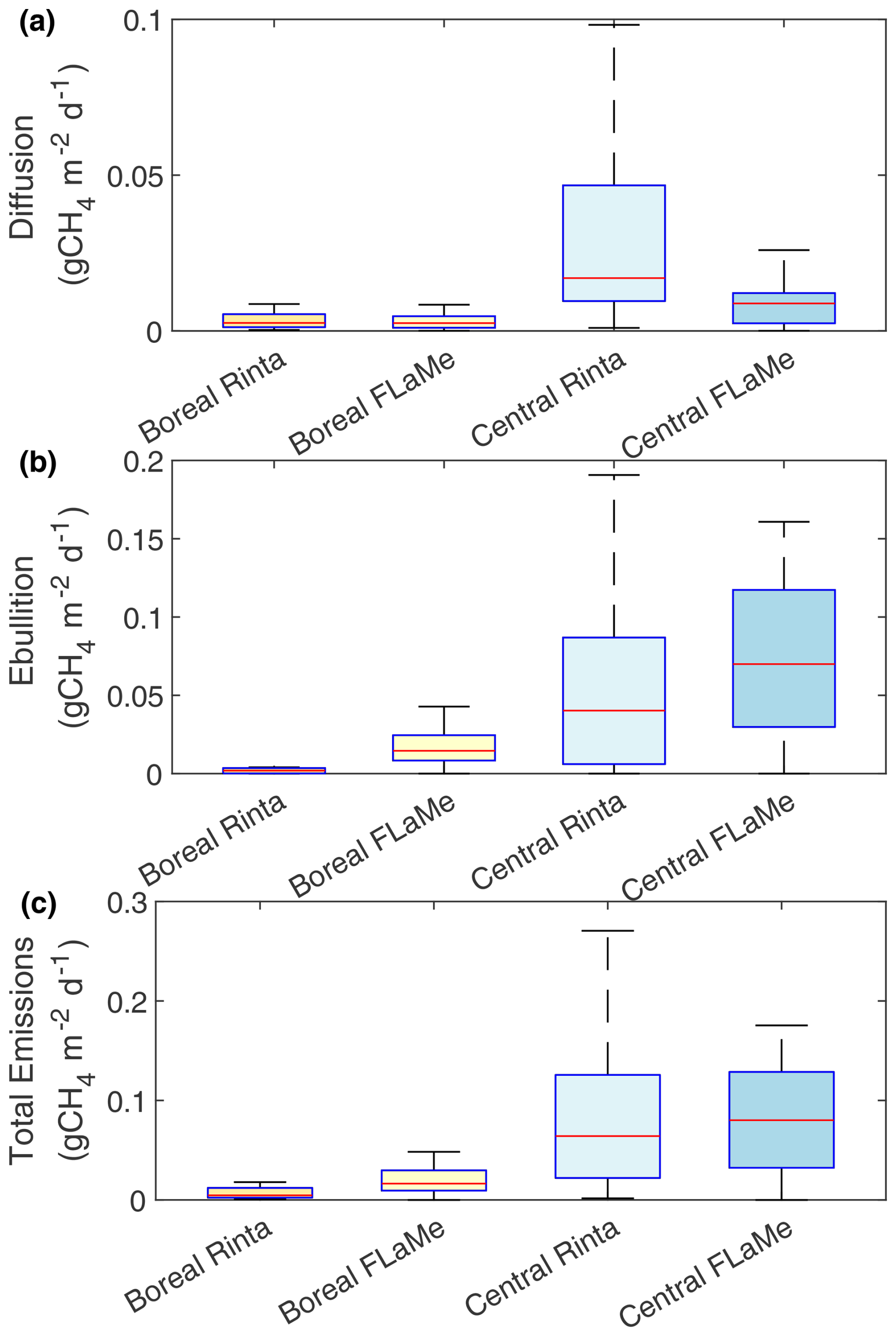
Figure 8Comparison of simulated diffusive (top), ebullitive (middle) and total (bottom) CH4 emission rates with the measurements complied by Rinta et al. (2017). The datasets reported by Rinta et al. (2017) comprises the diffusive, ebullitive and total emission rates from 17 boreal lakes in Finland and Sweden and 30 lakes of central European lakes in The Netherlands, Germany and Switzerland. The boxes represent the 25 % and 75 % quartiles, and the whiskers cover the 95 % confidence intervals. The same figure with a log scale is presented in Fig. S19.
3.3.2 European scale assessment of lake CH4 emissions
The continental-scale assessment indicates that European lakes smaller than 1000 km2 have an annual mean emission of 0.97 Tg CH4 yr−1 from autochthonous phytoplankton production during the period of 2010–2016, of which 30 % and 70 % are through diffusive and ebullitive transport pathways, respectively (Figs. 9 and S20). Note that, by including the estimated emissions from European lakes larger than 1000 km2 with two different strategies (Sect. S5), we provide a back of the envelope estimate for the mean total annual emission as 1.03–1.10 Tg CH4 yr−1, which falls within the lower end of a previously reported range (0.9–2.5 Tg CH4 yr−1) (Petrescu et al. 2023; Lauerwald et al., 2023). The mean CH4 emission rates per unit lake area amounts to 7.39 g CH4 m−2 yr−1, while the mean CH4 emission rates per unit land surface area amounts to 0.054 g CH4 m−2 yr−1. Both emission rates decrease from South to North, despite the larger number of lakes and lake surface area in Northern Europe (Messager et al., 2016; Fig. S4). This south to north decrease can be explained by a much higher CH4 emission rate in the South of Europe (reaching 109.6 g CH4 m−2 yr−1) driven by much higher eutrophic status of southern lakes (together with higher temperatures), which outcompetes the effect of the larger lake area in the Scandinavian region and Finland (which contribute to ∼ 30 % of the European lake area). The ice-cover in northern lakes also contribute to the south-to-north gradient of CH4 emission rates, which is tested to decrease the European lake emissions by 7 %. This latitudinal pattern of CH4 emissions per unit lake area is broadly consistent with that reported by Johnson et al. (2022) based on observations.
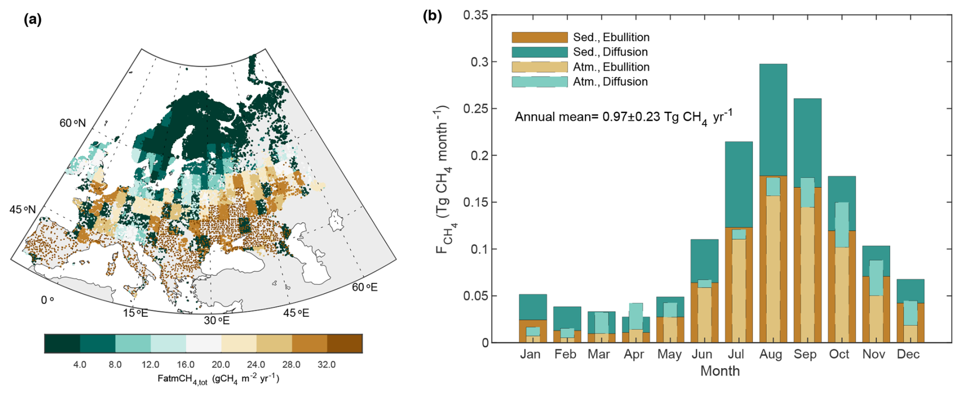
Figure 9Methane (CH4) emissions from European lakes. (a) Spatial distribution of annual mean total CH4 emissions (sum of diffusion and ebullition) for the period of 2010–2016, expressed in per unit of lake area. (b) Seasonality of total CH4 production (wide bars with full lines) and emission (narrow bars with dashed lines) fluxes and their split between ebullitive and diffusive pathways (period 2010–2016).
In terms of seasonal variability, our model results are in full agreement with the sparse data set of seasonally resolved observations (Tan et al., 2015) and show that European lakes as a whole act as a continuous CH4 source including during the winter months (individual lakes during ice-covered periods will do not emit CH4). Moreover, the simulated CH4 production and emission reveal a sharp 10-fold increase from late Spring to late Summer that is largely driven by the increase in ambient temperature and FPP rates. These findings underscore the importance of accounting for seasonal variations in CH4 emissions when refining regional methane budgets (Tan et al., 2015; Guo et al., 2020; Johnson et al., 2022; Stavert et al., 2021). A simple extrapolation of observed summer emissions to the yearly timescale would thus lead to an overestimation of yearly mean fluxes. In addition, model results also reveal a slight time-lag between the most favorable climate conditions (air temperature and light) and the maximum CH4 production. This time lag in the model can be explained by the cascade of biogeochemical reactions (primary production, mineralization, O2 depletion and onset of CH4 production) that ultimately control benthic CH4 fluxes, and the timescale of heat transfer from the lake surface to the deepest portion of our valley-shape lake bottom. This slight time-lag is further amplified by the time required for the benthic CH4 to reach the water-air interface, although this effect is secondary due to the dominance of shallow lakes (with mean depth < 7.8 m for 90 % of lakes; Messager et al., 2016) within the European domain. Finally, the broad seasonal pattern in CH4 emissions is complicated by the episodic releases of storage fluxes during lake turnovers which occur during spring (March and April; emissions > production) and fall (October and November; emission circa 85 % of the production). Lake turnovers amplify total emissions for the duration of these short-lived events.
3.3.3 Sensitivity and uncertainty analysis
The sensitivity analysis of annual mean CH4 emissions from European lakes to key model parameters (indicated by asterisks in Table 1) are summarized in Table 3. Table 3 indicates that the fraction of benthic organic matter mineralization channeled to methanogenesis (fmm) is the most sensitive parameter, and the increase (decrease) of fmm by one SD leads to an increase (decrease) of European lake CH4 emissions by 0.92 Tg CH4 yr−1 or 95 % (0.67 Tg CH4 yr−1 or 69 %). This is intuitive as a higher fraction of carbon channeled to methanogenesis will increase the continental scale CH4 emissions, although the response is nonlinear. This is also supported by the findings of high potential methane production rates in various freshwater systems (including the lakes, reservoirs and rivers) (Bodmer et al., 2025). The second and third most sensitive parameters are the maximum carbon fixation rate per unit of Chlorophyll a (Pchl,max) and the half saturation constant of phosphorus (Ks,P). An increase (decrease) of Pchl,max by one SD could increase (decrease) the European lake CH4 emissions by 0.77 Tg CH4 yr−1 or 79 % (0.63 Tg CH4 yr−1 or 65 %). This is again logical as a higher Pchl,max indicates a stronger capacity of phytoplankton to assimilate carbon, thus resulting in higher amounts of organic carbon available for CH4 production and emissions. The increase (decrease) of Ks,P by one SD decreases (increases) the European lake CH4 emissions by 0.46 Tg CH4 yr−1 or 48 % (0.22 Tg CH4 yr−1 or 22 %), a result which can be explained by a stronger TP limitation of primary production when Ks,P increases, resulting in lower CH4 production and emissions. The next most sensitive parameters are the mineralization and burial rates (k20 and kbur), for which an increase (decrease) in k20 by one SD result in an increase (decrease) of European lake CH4 emissions by 0.19 Tg CH4 yr−1 or 20 % (0.39 Tg CH4 yr−1 or 40 %), while an increase (decrease) of kbur by one SD leads to a decrease (increase) of European lake CH4 emissions by 0.35 Tg CH4 yr−1 or 36 % (0.21 Tg CH4 yr−1 or 22 %). This is straightforward to interpret as a higher mineralization rate (k20) will channel more mineralization into methanogenesis (and also via lower O2 levels in the lake), while a higher burial rate (kbur) translates to a lower relative amount of organic matter degradation, and thus lower CH4 production and emissions.
Table 3Sensitivity of European lake CH4 emissions (Tg CH4 yr−1) to key model parameters. Mean and SD are the mean and standard deviation of a particular parameter. Mean ±SD indicates that the parameter values are adjusted by ±one SD; Mean ±0.5 SD indicates that the parameter values are adjusted by ±0.5 SD.
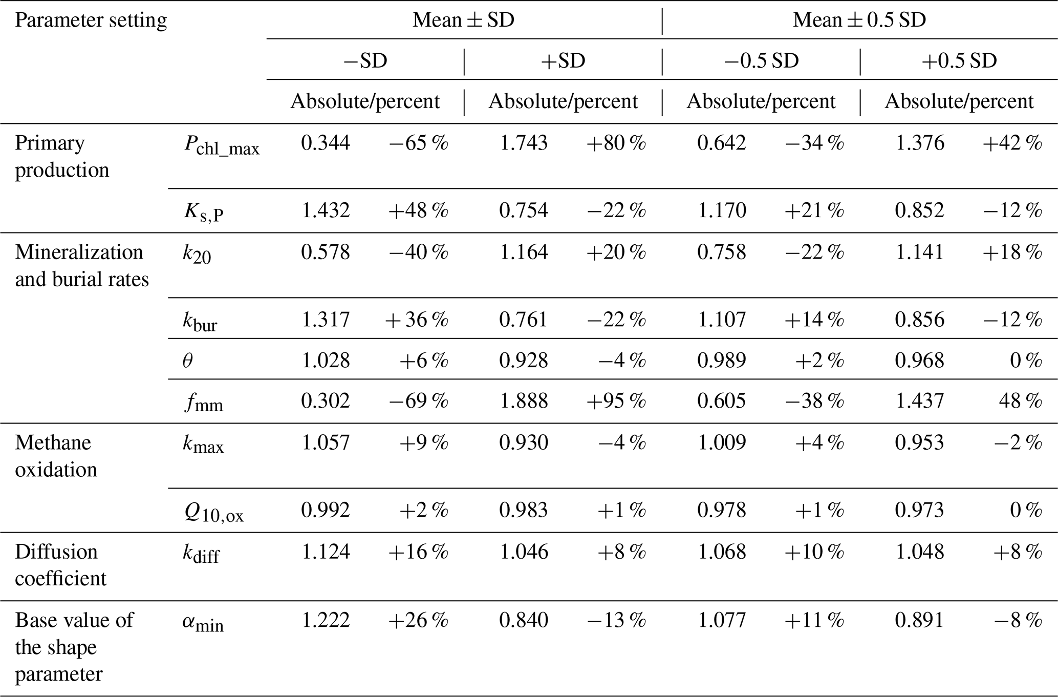
The other parameters (including the shape parameter of the CH4 production rate versus sediment depth αmin, the temperature dependence of mineralization θ, as well as the maximum CH4 oxidation rate kmax and its temperature dependence Q10,ox) are less sensitive, with their relative effects on European lake CH4 emissions ranging from 1 %–20 %. The shape parameter αmincan affect the CH4 emissions as it determines the split between diffusive and ebullitive pathways, i.e., a higher αmin favors a higher fraction of CH4 emitted to water and atmosphere through the diffusive pathway, a pathway that is more prone to oxidation thus lowering total CH4 emissions. We also find that a higher temperature dependence of mineralization (θ) results in a lower CH4 emission. This can be explained by the reference temperature of 20 °C in the expression of the θ function, higher than the mean water temperature in most lakes, leading to a faster drop in mineralization for a larger θ when temperature is lower than 20 °C. The parameter kmax barely impacts the total CH4 emissions, as this parameter mostly influences the thickness of the water layers where the profiles of oxygen and methane overlap and the oxidation occurs, while the volume-integrated rates remain essentially unaltered Thullner and Regnier, 2019; Grossart et al., 2011). As for the temperature dependence of oxidation (Q10,ox), the sensitivity is even weaker because changing the Q10,ox value has a lower impact on the oxidation rates than changing kmax. Compared to other parameters (such as fmm and Pchl,max), the relatively low effects of kmax and Q10,ox does not mean that the methane oxidation is not important, but highlight the dominant role of organic carbon production and decomposition on lake CH4 emissions, which were seldom simulated in previous models. Note that in our current model version, CH4 oxidation only occurs through the aerobic pathway and thus neglects the potential additional controls induced by anaerobic pathways (Regnier et al., 2011; Mostovaya et al., 2022; Su et al., 2020; Regnier et al., 2011).
With the samples produced by the above sensitivity analysis and complemented by samples from additional tests, we utilized a Random Forest (RF) model to assess the uncertainty of European lake CH4 emissions (see details in Sect. 2.5.4). The RF model has a R2 of 0.73 and Root of Mean Square Error (RMSE) of 0.24 Tg CH4 yr−1 for the train set (Fig. 10a) and a R2 of 0.52 and RMSE of 0.30 Tg CH4 yr−1 for the out-of-bag samples (Fig. 10b), suggesting that it can capture the relationship between model parameters and European lake CH4 emissions well. Using these ensembles of CH4 emissions, the uncertainty (or SD) of European lake CH4 emissions associated with the choice of biogeochemical parameter values was estimated as 0.23 Tg CH4 yr−1. Therefore, during the period of 2010–2016, the European lakes (with surface areas between 0.1–1000 km2) have an annual mean emission of 0.97 ± 0.23 Tg CH4 yr−1.
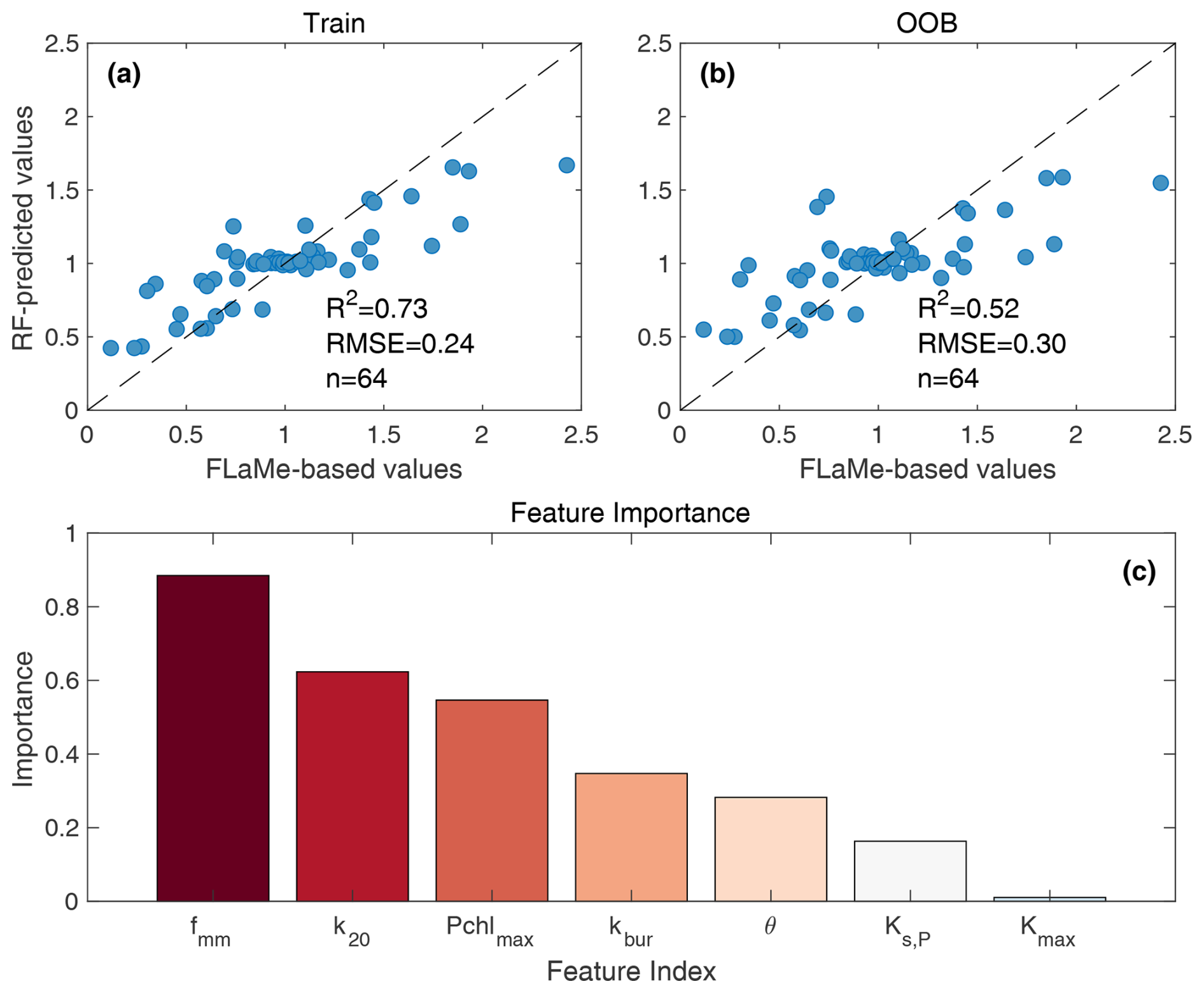
Figure 10Random Forest (RF) model for the uncertainty analysis. (a) and (b) are the train and test (Out-of-Bag prediction) of the RF model. (c) shows the importance of key model parameters. Note that the parameters of αmin and Q10,ox are excluded from illustration due to their second order of importance (indicated by negative values).
With the RF model, we can also identify the importance of key model parameters involved as predictors (Fig. 10c). We noticed that the first four leading parameters are also the most sensitive parameters as identified in Table 3, while the importance of other parameters are slightly different from the sensitivity analysis. This slight difference can be attributed to the interactions of model parameters that are overlooked in the sensitivity analysis. Overall, from the sensitivity and uncertainty analysis, we find that the European lake CH4 emissions are strongly controlled by the carbon biogeochemical dynamics, which, however, was not fully accounted for in previous lake models.
We have illustrated that FLaMe-v1.0 is able to capture complex physical-biogeochemical behaviors for lakes with diverse settings and environmental controls. Specifically, the FLaMe-v1.0 has been evaluated against (i) observational temporal variations of CH4 fluxes at four contrasting, well-surveyed real lakes, (ii) the empirical ranges of primary production under different trophic status reported by Wetzel (2001), and (iii) observational patterns of CH4 emissions against trophic and climate gradients spanning the European domain (Rinta et al., 2017). Moreover, the European scale simulation produces a spatial pattern of lake CH4 emission rates consistent with observation-based upscaling approaches (Johnson et al., 2022). This continental scale application also demonstrates the power of our modelling framework that rests on a lake clustering approach and on a routing of nutrient (TP) inputs from surrounding catchments to lakes that allow to account for eutrophication effects. Our results thus suggest that the FLaMe-v1.0 modelling framework performs well in providing reliable spatio-temporal patterns of lake CH4 emissions at the regional scale (with lake areas < 1000 km2). However, the results also pinpoint to several key aspects to be improved in the model and highlight critical data gaps that must be addressed in the future.
First, the organic carbon module only accounts for autochthonous OC production as the substrate for methanogenesis, but ignores the contribution of allochthonous OC inputs leached from the catchments, rivers and streamflow. This is based on the distinct reactivity of autochthonous vs. allochthonous OC inputs, with the latter being more refractory to mineralization and decomposition. As a result, FLaMe-v1.0 may provide conservative estimates of CH4 production and emission. However, neglecting the allochthonous C inputs may at the same time minimize the feedback of OC on light penetration, leading to systematically biased estimates of autochthonous production (see Organic carbon module). Moreover, transient lake phosphorus dynamics and the co-limitations by nitrogen, albeit assumed to be less important, are neglected and might increase the uncertainty in the estimates of CH4 production and emission. In addition, our primary production model does not resolve the short-term (e.g., (sub)daily) dynamics of algae growth induced by climate variability, rendering model-data comparison more difficult. In future model developments, these limitations could be addressed by (i) integrating or routing the lake water, carbon and nutrient fluxes along the global river network, which would allow to simultaneously solve the issue of time-invariant lake water levels in current global lake models (Golub et al., 2022), including ours; (ii) refining the carbon module by incorporating more dynamic models for algal growth as well as P and N uptake and recycling processes within lakes.
Second, several model assumptions and implementations are based on empirical or theoretical knowledge, which may lead to biases in the estimation of CH4 fluxes. For instance, the present version of FLaMe (i.e., v1.0) neglects the plant-mediated emission pathway (through aerenchyma in rooted plant) in the littoral zone (Mayr et al., 2020; Zimmermann et al., 2019) due to the lack of observational data for model calibration. Moreover, a recently reported process, i.e., the horizontal, advective littoral-pelagic transport of oxygen and methane (Doda et al., 2024; Bouffard et al., 2025) was ignored for the following reasons: (1) The current FLaMe-v1.0 relies on a 1-D vertical representation while explicitly accounting for horizontal transport would require a 2-D framework; and (2) observations related to horizontal transport remain limited, and whether this is an ubiquitous feature of the CH4 dynamics across a wide range of lakes will require further observational evidences. Furthermore, in our model, the lake is assumed to follow a “valley” shape. Although this is an advancement from the “bucket” shape used in previous process-based lake models of CH4 emissions (e.g., LAKE 2.0, ABLM, and bLake4Me), it remains a simplified assumption that captures important but not all features of a realistic lake geometry. Furthermore, several benthic CH4 processes are highly parameterized. For instance, the split between aerobic and anaerobic decomposition of organic matter is represented by a single parameter fmm and is determined based on the data compilation from Bastviken (2022). This simplification leads to the same temperature dependence of CH4 processes occurring in the sediment as that of pelagic and benthic mineralization. This is a shortcoming although it should be noted that the overall temperature dependence of CH4 emissions, which results from the combined effects of OC production, mineralization, and subsequent CH4 processes, was found to fall well within the observed ranges reported by Aben et al. (2017) (Fig. S21). The split of diffusive and ebullitive CH4 fluxes is also currently captured by an empirically determined threshold depth (zeb,min) based on limited observations by Langenegger et al. (2019). Moreover, the effects of heat transfer and CH4 bubbles migration in the sediment are not resolved, which may lead to biased simulation of CH4 fluxes especially for the timing. These are simplified representations related to the highly complex pathways of CH4 production and emission, which needs to be improved by more mechanistic representations of the biogeochemical processes controlling carbon cycling, CH4 production and transport via diffusion and bubble ascent. In addition, we acknowledge that the fixed grid spacing currently limits the model application to very shallow lakes, which could be solved by adopting a variable grid spacing scaling to the maximum lake depth.
Third, different modules of the FLaMe-v1.0 could benefit from more comprehensive calibration and evaluation but those are limited by data availability. Although FLaMe-v1.0 has been evaluated against several timeseries of observed data collected in four well-surveyed lakes with contrasted dynamics, a full evaluation in the context of large-scale application would benefit from a significantly larger and representative set of observational data. Moreover, the in-situ climate conditions may vary greatly from the grid-level forcings, and the lake water dynamics may also affect the CH4 fluxes significantly (e.g., Upper Mystic Lake; Varadharajan, 2009). Thus, a full comprehensive set of in-situ measurements of climate, water level, physical and biogeochemical variables would be highly valuable for the purpose of further model development, calibration and evaluation. At the European scale, we partly circumvented these limitations by evaluating lake primary production against the broad ranges reported by Wetzel (2001), and the simulated diffusive and ebullitive CH4 fluxes across the environmental (nutrient and climate) gradients compiled by Rinta et al. (2017). In this context, complementary time-series of vertically resolved organic carbon, CH4 and O2 concentrations, as well as high frequency measurements of CH4 fluxes capturing short-lived emissions via the storage and ebullitive pathways and covering heterogeneity of CH4 fluxes in large lakes (Denfeld et al., 2018; Mayr et al., 2020; Zimmermann et al., 2019) would help further calibrate and evaluate the FLaMe-v1.0. These measurements should be performed using a sufficiently large set of representative lakes covering the full range of lake morphologies, landscape properties, and climate.
In this study, we developed and tested a new process-based biogeochemical modeling framework (FLaMe-v1.0) to simulate lake CH4 fluxes on the large-scale and, as a “proof of concept”, applied the model to European lakes. The physical lake model builds on the Canadian Small Lake Model (CSLM) and is coupled to a set of novel biogeochemical modules describing lake organic matter, oxygen and methane dynamics. We then showcased the abilities and performance of FLaMe-v1.0 by: (1) analyzing the overall behaviors of the coupled C-O2-CH4 dynamics in two representative cases (a deep oligotrophic lake driven by cold climate in Northern Europe and a shallow eutrophic lake driven by warm climate in Southern Europe) as well as their decomposition, and (2) evaluating simulated temporal patterns of CH4 fluxes against observations at four well-surveyed lakes with long-term timeseries. Simulation results were consistent with our common knowledge of lake CH4 dynamics, suggesting that FLaMe-v1.0 can capture the patterns of CH4 production and emissions across different lake types as well as their responses to the changes in environment conditions, despite the complexity of underlying biogeochemical processes. Furthermore, by applying the model to boreal and central European lakes, we showed that FLaMe-v1.0 captures well the observed magnitudes of both diffusive and ebullitive CH4 fluxes as well as the difference between boreal and central lakes. Finally, at the European scale, FLaMe-v1.0 estimates total CH4 emissions from lakes with areas of 0.1–1000 km2 (n= 108 407, total area = 1.33 × 10⁵ km2) as 0.97 ± 0.23 Tg CH4 yr−1. In addition, the model resolves spatial patterns and seasonal variations of CH4 emissions, providing a comprehensive view of their contribution to regional methane budgets.
Despite some limitations in its current model configuration, this first version of FLaMe is a significant step forward in biogeochemical simulations of lake CH4 dynamics. The model explicitly incorporates the dynamics of volume-integrated organic carbon cycling, such that the responses of organic carbon to climate and environmental change can be accounted for in estimating CH4 emissions. We also have incorporated the primary production as a function of total phosphorus loads from the surrounding catchments, allowing us to evaluate for the first time the impact of eutrophication on CH4 emissions in a quantitative way. Moreover, our model is of intermediate complexity, and is thus designed for large scale applications. Although the model was run here at a coarse spatial resolution, its parallelized version offers the possibility to carry simulations at a finer resolution in the future. With these advancements, our model can be used to resolve the spatio-temporal variability of CH4 emissions at regional and global scales under past and future climates, and has the potential to be coupled to Earth System Models to investigate the feedback between climate warming and global lake CH4 emissions.
The source codes for FLaMe (Fluxes of Lake Methane) model version 1.0 are available at: https://doi.org/10.5281/zenodo.16881039, Feng (2025).
The methane emission data for the four well-surveyed real lakes (Klöntal, Erssjön, Upper Mystic, and Villasjön) were obtained from Tan et al. (2024). The in-situ measurements of diffusive and ebullitive CH4 emission rates in boreal and central European regions during late summer (August–September 2010–2011) were obtained from Rinta et al. (2017). The lake characteristic information within Europe were obtained from the HydroLAKES database (Messager et al., 2016): https://www.hydrosheds.org/products/hydrolakes (last access: 23 July 2023). The meteorological variables from GSWP3-W5E5 reanalysis product were obtained from Inter-Sectoral Impact Model Intercomparison Project (ISIMIP3a): https://www.isimip.org/gettingstarted/input-data-bias-adjustment/ (last access: 29 July 2023).
The supplement related to this article is available online at https://doi.org/10.5194/esd-16-1779-2025-supplement.
MM, MF and PR designed the study as well as the overall model strategy. MM and MF co-developed and tested the FLaMe model. DB, SA, RL, AJ, GGL, MDM, and ZT provided plenty of valuable suggestions related to the model development. DB and SA also provided constructive suggestions on model evaluation against measurements and manuscript writing. MDM helped us in setting up the CSLM at the beginning of developing FLaMe, ZT provided us the methane emission data from ISIMIP lake datasets, and WT helped us in collecting climate forcings from ISIMIP3a. MM and MF wrote the first version of the manuscript, and all coauthors helped in improving the manuscript.
The contact author has declared that none of the authors has any competing interests.
Publisher’s note: Copernicus Publications remains neutral with regard to jurisdictional claims made in the text, published maps, institutional affiliations, or any other geographical representation in this paper. While Copernicus Publications makes every effort to include appropriate place names, the final responsibility lies with the authors. Also, please note that this paper has not received English language copy-editing. Views expressed in the text are those of the authors and do not necessarily reflect the views of the publisher.
This study was supported by the Fonds National de la Recherche Scientifique of Belgium (F.R.S.–FNRS PDR T.0191.23), by the project CLIMATE-SPACE RECCAP2: Global Land Carbon Budget and its Attribution to regional drivers, and by the project ESM2025–Earth System Models for the Future (grant no. 101003536). David Bastviken acknowledges support from the European Research Council (ERC H2020; grant no. 725546), the Swedish Research Councils VR (grant nos. 2016-04829 and 2022-03841), and Formas (grant no. 2018-01794). Sandra Arndt acknowledges funding from the F.R.S.–FNRS under grant no. 35266740 (FIESTA). Ronny Lauerwald acknowledges funding from French state aid, managed by ANR under the “Investissements d'avenir” programme (ANR-16-CONV-0003) and under the “France 2030” programme (ANR-22-PEXF-0009, i.e. PEPR FairCarboN – project “DEEP-C”. Goulven Gildas Laruelle is research associate of the F.R.S–FNRS at the Université Libre de Bruxelles. Zeli Tan was supported by the US DOE’s Earth System Modeling program through the Energy Exascale Earth System Model (E3SM) project. The Pacific Northwest National Laboratory is operated by Battelle for the U.S. Department of Energy under Contract DE-AC05-76RLO1830. We acknowledge the climate modelling groups involved in ISIMIP3a for producing and making available their model outputs. Computational resources have been provided by the Consortium des Équipements de Calcul Intensif (CÉCI), funded by the Fonds de la Recherche Scientifique de Belgique (F.R.S.–FNRS) under grant no. 2.5020.11 and by the Walloon Region. Correspondence and requests for materials should be addressed to Maoyuan Feng (Maoyuan.feng@ulb.be).
This study was supported by the Fonds National de la Recherche Scientifique of Belgium (F.R.S.–FNRS PDR T.0191.23), by the project CLIMATE-SPACE RECCAP2: Global Land Carbon Budget and its Attribution to regional drivers, and by the project ESM2025–Earth System Models for the Future (grant no. 101003536). David Bastviken acknowledges support from the European Research Council (ERC H2020; grant no. 725546), the Swedish Research Councils VR (grant nos. 2016-04829 and 2022-03841), and Formas (grant no. 2018-01794). Sandra Arndt acknowledges funding from the F.R.S.–FNRS under grant no. 35266740 (FIESTA). Ronny Lauerwald acknowledges funding from French state aid, managed by ANR under the “Investissements d'avenir” programme (ANR-16-CONV-0003) and under the “France 2030” programme (ANR-22-PEXF-0009, i.e. PEPR FairCarboN – project “DEEP-C”. Goulven Gildas Laruelle is research associate of the F.R.S–FNRS at the Université Libre de Bruxelles. Zeli Tan was supported by the US DOE’s Earth System Modeling program through the Energy Exascale Earth System Model (E3SM) project. The Pacific Northwest National Laboratory is operated by Battelle for the U.S. Department of Energy under Contract DE-AC05-76RLO1830. We acknowledge the climate modelling groups involved in ISIMIP3a for producing and making available their model outputs. Computational resources have been provided by the Consortium des Équipements de Calcul Intensif (CÉCI), funded by the Fonds de la Recherche Scientifique de Belgique (F.R.S.–FNRS) under grant no. 2.5020.11 and by the Walloon Region.
This paper was edited by Parvadha Suntharalingam and reviewed by two anonymous referees.
Aben, R. C. H., Barros, N., van Donk, E., Frenken, T., Hilt, S., Kazanjian, G., Lamers, L. P. M., Peeters, E. T. H. M., Roelofs, J. G. M., de Senerpont Domis, L. N., Stephan, S., Velthuis, M., Van de Waal, D. B., Wik, M., Thornton, B. F., Wilkinson, J., DelSontro, T., and Kosten, S.: Cross continental increase in methane ebullition under climate change, Nat. Commun., 8, 1682, https://doi.org/10.1038/s41467-017-01535-y, 2017.
Arístegui, J., Agustí, S., and Duarte, C. M.: Respiration in the dark ocean, Geophys. Res. Lett., 30, 1041, https:///doi.org/10.1029/2002GL016227, 2003.
Bastviken, D.: Methane, in: Encyclopedia of inland waters (Second Edition), edited by: Mehner, T. and Tockner, K., Oxford, Elsevier, 136–154, https://doi.org/10.1016/B978-0-12-819166-8.00147-X, 2022.
Bastviken, D., Cole, J., Pace, M., and Tranvik, L.: Methane emissions from lakes: Dependence of lake characteristics, two regional assessments, and a global estimate, Global Biogeochem. Cycles, 18, GB4009, https//doi/org/10.1029/2004GB002238, 2004.
Bastviken, D., Tranvik L. J., Downing, J. A., Crill, P. M., and Enrich-Prast, A.: Freshwater methane emissions offset the continental carbon sink, Science, 331, 50, https//doi/org/10.1126/science.1196808, 2011.
Behrenfeld, M. J. and Falkowski P. G.: Photosynthetic rates derived from satellite-based chlorophyll concentration, Limnol. Oceanogr., 42, https//doi/org/10.4319/lo.1997.42.1.0001, 1997.
Bodmer, P., Bors, C., Liu, L., and Lorke, A.: Large sediment methane production potential in reservoirs compared to lakes and rivers, Limnol. Oceanogr., https://doi.org/10.1002/lno.70063, 2025.
Boehrer, B. and Schultze, M.: Stratification of lakes, Rev. Geophys., 46, 2006RG000210, https://doi.org/10.1029/2006RG000210, 2008.
Bouffard, D., Doda, T., Ramón, C. L., and Ulloa, H. N.: Thermally driven cross-shore flows in stratified basins: a review on the thermal siphon dynamics, Flow, 5, https://doi.org/10.1017/flo.2024.31, 2025.
Bouwman, A. F., Beusen, A. H. W., and Billen G.: Human alteration of the global nitrogen and phosphorus soil balances for the period 1970–2050, Global Biogeochem. Cycles, 23, GB0A04, https//doi/org/10.1029/2009GB003576, 2009.
Canadell, J. G., Monteiro, P. M. S., Costa, M. H., Cotrim da Cunha, L., Cox, P. M., Eliseev, A. V., Henson, S., Ishii, M., Jaccard, S., Koven, C., Lohila, A., Patra, P. K., Piao, S., Rogelj, J., Syampungani, S., Zaehle, S., and Zickfeld, K.: Global carbon and other biogeochemical cycles and feedbacks, In: Climate Change 2021: The Physical Science Basis: Working Group I Contribution to the Sixth Assessment Report of the Intergovernmental Panel on Climate Change, edited by: Masson-Delmotte, V., Zhai, P., Pirani, A., Connors, S. L., Péan, C., Berger, S., Caud, N., Chen, Y., Goldfarb, L., Gomis, M. I., Huang, M., Leitzell, K., Lonnoy, E., Matthews, J. B. R., Maycock, T. K., Waterfield, T., Yelekçi, O., Yu, R., and Zhou B., Cambridge University Press, Cambridge, United Kingdom and New York, NY, USA, 673–816, https//doi/org/10.1017/9781009157896.007, 2021.
Carlson, C. A., Ducklow, H. W., and Michaels, A. F.: Annual flux of dissolved organic carbon from the euphotic zone in the northwestern Sargasso Sea, Nature, 397, 405–408, https://doi.org/10.1038/371405a0, 1994.
Cole, J. J. and Caraco, N. F.: Atmospheric exchange of carbon dioxide in a low-wind oligotrophic lake measured by the addition of SF6, Limnol. Oceanogr., 4, https//doi/org/ 10.4319/lo.1998.43.4.0647, 1998.
Deemer, B. R. and Holgerson, M. A.: Drivers of methane flux differ between lakes and reservoirs, complicating global upscaling efforts, J. Geophys. Res.-Biogeo., 126, e2019JG005600, https://doi.org/10.1029/2019JG005600, 2021.
Deemer, B. R., Harrison, J. A., Li, S., Beaulieu, J. J., DelSontro, T., Barros, N., Bezerra-Neto, J. F., Powers, S. M., dos Santos, M. A., and Vonk, J. A.: Greenhouse gas emissions from reservoir water surfaces: A new global synthesis, Bioscience, 66, 949–964, https//doi/org/ 10.1093/biosci/biw117, 2016.
DelSontro, T., Beaulieu, J. J., and Downing, J. A.: Greenhouse gas emissions from lakes and impoundments: Upscaling in the face of global change, Limnol. Oceanogr. Lett., 3, 64–75, https://doi.org/10.1002/lol2.10073, 2018.
Delwiche, K. and Hemond, H. F.: An enhanced bubble size sensor for long-term ebullition studies, Limnol. Oceanogr. Methods, 15, 821–835, https://doi.org/10.1002/lom3.10201, 2017
Denfeld, B. A., Baulch, H. M., del Giorgio, P. A., Hampton, S. E., and Karlsson, J.: A synthesis of carbon dioxide and methane dynamics during the ice-covered period of northern lakes, Limnol. Oceanogr. Lett., 3, 117–131, https://doi.org/10.1002/lol2.10079, 2018.
Doda, T., Ramón, C. L., Ulloa, H., N., Brennwald, M. S., Kipfer, R., Perga M.-E., Wüest, A., Schubert, C. J., and Bouffard, D.: Lake surface cooling drives littoral-pelagic exchange of dissolved gases, Sci. Adv., 10, eadi0617, https//doi/org/10.1126/sciadv.adi0617, 2024.
Dong, J., Fox-Kemper, B., Zhang, H., and Dong, C.: The Scale of Submesoscale Baroclinic Instability Globally, J. Phys. Oceanogr., 50, 2649–2667, https://doi.org/10.1175/JPO-D-20-0043.1, 2020.
Feng, M.: myFeng818/FLaMe-model-v1.0: FLaMe-model-v1.0 (v1.0), Zenodo [code], https://doi.org/10.5281/zenodo.16881039, 2025.
Frieler, K., Volkholz, J., Lange, S., Schewe, J., Mengel, M., del Rocío Rivas López, M., Otto, C., Reyer, C. P. O., Karger, D. N., Malle, J. T., Treu, S., Menz, C., Blanchard, J. L., Harrison, C. S., Petrik, C. M., Eddy, T. D., Ortega-Cisneros, K., Novaglio, C., Rousseau, Y., Watson, R. A., Stock, C., Liu, X., Heneghan, R., Tittensor, D., Maury, O., Büchner, M., Vogt, T., Wang, T., Sun, F., Sauer, I. J., Koch, J., Vanderkelen, I., Jägermeyr, J., Müller, C., Rabin, S., Klar, J., Vega del Valle, I. D., Lasslop, G., Chadburn, S., Burke, E., Gallego-Sala, A., Smith, N., Chang, J., Hantson, S., Burton, C., Gädeke, A., Li, F., Gosling, S. N., Müller Schmied, H., Hattermann, F., Wang, J., Yao, F., Hickler, T., Marcé, R., Pierson, D., Thiery, W., Mercado-Bettín, D., Ladwig, R., Ayala-Zamora, A. I., Forrest, M., and Bechtold, M.: Scenario setup and forcing data for impact model evaluation and impact attribution within the third round of the Inter-Sectoral Impact Model Intercomparison Project (ISIMIP3a), Geosci. Model Dev., 17, 1–51, https://doi.org/10.5194/gmd-17-1-2024, 2024.
Forster, P. M., Smith, C., Walsh, T., Lamb, W. F., Lamboll, R., Hall, B., Hauser, M., Ribes, A., Rosen, D., Gillett, N. P., Palmer, M. D., Rogelj, J., von Schuckmann, K., Trewin, B., Allen, M., Andrew, R., Betts, R. A., Borger, A., Boyer, T., Broersma, J. A., Buontempo, C., Burgess, S., Cagnazzo, C., Cheng, L., Friedlingstein, P., Gettelman, A., Gütschow, J., Ishii, M., Jenkins, S., Lan, X., Morice, C., Mühle, J., Kadow, C., Kennedy, J., Killick, R. E., Krummel, P. B., Minx, J. C., Myhre, G., Naik, V., Peters, G. P., Pirani, A., Pongratz, J., Schleussner, C.-F., Seneviratne, S. I., Szopa, S., Thorne, P., Kovilakam, M. V. M., Majamäki, E., Jalkanen, J.-P., van Marle, M., Hoesly, R. M., Rohde, R., Schumacher, D., van der Werf, G., Vose, R., Zickfeld, K., Zhang, X., Masson-Delmotte, V., and Zhai, P.: Indicators of Global Climate Change 2023: annual update of key indicators of the state of the climate system and human influence, Earth Syst. Sci. Data, 16, 2625–2658, https://doi.org/10.5194/essd-16-2625-2024, 2024.
Garnaud, C., MacKay, M., and Fortin, V.: A one-dimensional lake model in ECCC's land surface prediction system, J. Adv. Model. Earth Sy., 14, e2021MS002861, https://doi.org/10.1029/2021MS002861, 2022.
Gatley, D. P., Herrmann, S., and Kretzschmar, H. J.: A twenty-first century molar mass for dry air, HVAC&R Research, 14, 655–66, https://doi.org/10.1080/10789669.2008.10391032, 2008.
Golub, M., Thiery, W., Marcé, R., Pierson, D., Vanderkelen, I., Mercado-Bettin, D., Woolway, R. I., Grant, L., Jennings, E., Kraemer, B. M., Schewe, J., Zhao, F., Frieler, K., Mengel, M., Bogomolov, V. Y., Bouffard, D., Côté, M., Couture, R.-M., Debolskiy, A. V., Droppers, B., Gal, G., Guo, M., Janssen, A. B. G., Kirillin, G., Ladwig, R., Magee, M., Moore, T., Perroud, M., Piccolroaz, S., Raaman Vinnaa, L., Schmid, M., Shatwell, T., Stepanenko, V. M., Tan, Z., Woodward, B., Yao, H., Adrian, R., Allan, M., Anneville, O., Arvola, L., Atkins, K., Boegman, L., Carey, C., Christianson, K., de Eyto, E., DeGasperi, C., Grechushnikova, M., Hejzlar, J., Joehnk, K., Jones, I. D., Laas, A., Mackay, E. B., Mammarella, I., Markensten, H., McBride, C., Özkundakci, D., Potes, M., Rinke, K., Robertson, D., Rusak, J. A., Salgado, R., van der Linden, L., Verburg, P., Wain, D., Ward, N. K., Wollrab, S., and Zdorovennova, G.: A framework for ensemble modelling of climate change impacts on lakes worldwide: the ISIMIP Lake Sector, Geosci. Model Dev., 15, 4597–4623, https://doi.org/10.5194/gmd-15-4597-2022, 2022.
Grasset, C., Mendonça, R., Villamor Saucedo, G., Bastviken, D., Roland, F., and Sobek, S.: Large but variable methane production in anoxic freshwater sediment upon addition of allochthonous and autochthonous organic matter. Limnol. Oceanogr., 63, 1488–1501, https://doi.org/10.1002/lno.10786, 2018.
Grossart, H., Frindte, K., Dziallas, C., Eckert, W., and Tang, K. W.: Microbial methane production in oxygenated water column of an oligotrophic lake, P. Natl. Acad. Sci. USA, 108, 19657–19661, https://doi.org/10.1073/pnas.1110716108, 2011.
Guillemette, F., von Wachenfeldt, E., Kothawala, D. N., Bastviken, D., and Tranvik, L. J.: Preferential sequestration of terrestrial organic matter in boreal lake sediments, J. Geophys. Res.-Biogeo., 122, 863–874, https://doi.org/10.1002/2016JG003735, 2017.
Guildford, S. J. and Hecky, R. E.: Total nitrogen, total phosphorus, and nutrient limitation in lakes and oceans: Is there a common relationship? Limnology and Oceanography, 45, 1213–1223, https://doi.org/10.4319/lo.2000.45.6.1213, 2000.
Guo, M., Zhuang, Q., Tan, Z., Shurpali, N., Juutinen, S., Kortelainen, P., and Martikainen, P. J.: Rising methane emissions from boreal lakes due to increasing ice-free days. Environmental Research Letters, 15, 064008, https://doi.org/10.1088/1748-9326/ab8254, 2020.
Hanson, P. C., Hamilton, D. P., Stanley, E. H., Preston, N., Langman, O. C., and Kara, E. L.: Fate of allochthonous dissolved organic carbon in lakes: A quantitative Approach, PLoS One, 6, e21884, https://doi.org/10.1371/journal.pone.0021884, 2011.
Hanson, P. C., Buffam, I., Rusak, J. A., Stanley, E. H., and Watras, C.: Quantifying lake allochthonous organic carbon budgets using a simple equilibrium model, Limnol. Oceanogr., 59, https//doi.org/10.4319/lo.2014.59.1.0167, 2014.
Holgerson, M. and Raymond, P.: Large contribution to inland water CO2 and CH4 emissions from very small ponds, Nat. Geosci., 9, 222–226, https://doi.org/10.1038/ngeo2654, 2016.
Imberger, J.: The diurnal mixed layer, Limnol. Oceanogr., 30, 737–770, https://doi.org/10.4319/lo.1985.30.4.0737, 1985.
Imboden, D. M. and Wüest, A.: Mixing mechanisms in lakes, in: Physics and chemistry of lakes, edited by: Lerman, A., Imboden, D. M., and Gat, J. R., Springer, Berlin, Heidelberg, https://doi.org/10.1007/978-3-642-85132-2_4, 1995.
Jackson, R., Saunois, M., Bousquet, P., Canadell, J. G., Poulter, B., Stavert, A. R., Bergamaschi, P., Niwa, Y., Segers, A., and Tsuruta, A.: Increasing anthropogenic methane emissions arise equally from agricultural and fossil fuel sources, Environ. Res. Lett., 15, 071002, https://doi.org/10.1088/1748-9326/ab9ed2, 2020.
Jackson, R. B., Saunois, M., Martinez, A., Canadell, J. G., Yu, X., Li, M., Poulter, B., Raymond, P. A., Regnier, P., Ciais, P., Davis, S. J., and Patra, P. K.: Human activities now fuel two-thirds of global methane emissions, Environ. Res. Lett., 19, 101002, https://doi.org/10.1088/1748-9326/ad6463, 2024.
Johnson, M. S., Matthews, E., Du, J., Genovese, V., and Bastviken, D.: Methane emission from global lakes: New spatiotemporal data and observation-driven modeling of methane dynamics indicates lower emissions, J. Geophys. Res.-Biogeo., 127, e2022JG006793, https://doi.org/10.1029/2022JG006793, 2022.
Lan, X., Thoning, K. W., and Dlugokencky, E. J.: Trends in globally-averaged CH4, N2O, and SF6 determined from NOAA Global Monitoring Laboratory measurements, https://doi.org/10.15138/P8XG-AA10, 2024
Langenegger, T., Vachon, D., Donis, D., and McGinnis, D. F.: What the bubble knows: Lake methane dynamics revealed by sediment gas bubble composition, Limnol. Oceanogr., 64, 1526–1544, https://doi.org/10.1002/lno.11133, 2019.
Lauerwald, R., Regnier, P., Figueiredo, V., Enrich-Prast, A., Bastviken, D., and Lehner, B.: Natural lakes are a minor global source of N2O to the atmosphere, Global Biogeochem. Cycles, 33, 1564–1581, https://doi.org/10.1029/2019GB006261, 2019.
Lauerwald, R., Allen, G. H., Deemer, B. R., Liu, S., Maavara, T., Raymond, P., Alcott, L., Bastviken, D., Hastie, A., Holgerson, M. A., Johnson, M. S., Lehner, B., Lin, P., Marzadri, A., Ran, L., Tian, H., Yang, X., Yao, Y., and Regnier, P.: Inland water greenhouse gas budgets for RECCAP2: 2. Regionalization and homogenization of estimates, Global Biogeochem. Cycles, 37, e2022GB007658, https://doi.org/10.1029/2022GB007658, 2023.
Lewis, W. M.: Global primary production of lakes: 19th Baldi Memorial Lecture, Inland Waters, 1, 1–28, https://doi.org/10.5268/IW-1.1.384, 2011.
Liikanen, A., Murtoniemi, T., Tanskanen, H., Väisänen, T., and Martikainen, P. J.: Effects of temperature and oxygen availability on greenhouse gas and nutrient dynamics in sediment of a eutrophic mid-boreal lake, Biogeochemistry, 59, 269–286, https://doi.org/10.1023/A:1016015526712, 2002
Maavara, T., Lauerwald, R., Regnier, P., and Van Cappellen, P.: Global perturbation of organic carbon cycling by river damming, Nat. Commun., 8, 15347, https://doi.org/10.1038/ncomms15347, 2017.
Maavara, T., Lauerwald, R., Laruelle, G. G., Akbarzadeh, Z., Bouskill, N. J., Van Cappellen, P., and Regnier, P. Nitrous oxide emissions from inland waters: Are IPCC estimates too high?, Glob. Change Biol., 25, 473–448, https://doi.org/10.1111/gcb.14504, 2019.
MacKay, M. D.: A process–oriented small lake scheme for coupled climate modeling applications, J. Hydrometeorol., 13, 1911–1924, https://doi.org/10.1175/JHM-D-11-0116.1, 2012.
MacKay, M. D., Verseghy, D. L., Fortin, V., and Rennie, M. D.: Wintertime simulations of a boreal lake with the Canadian Small Lake Model, J. Hydrometeorol., 18, 2143–2160, https://doi.org/10.1175/JHM-D-16-0268.1, 2017.
MacIntyre, S., Bastviken, D., Arneborg, L., Crowe, A. T., Karlsson, J., Andersson, A., Gålfalk, M., Rutgersson, A., Podgrajsek, E. and Melack, J. M.: Turbulence in a small boreal lake: Consequences for air-water gas exchange, Limnol. Oceanogr., 66, 827–854, https://doi.org/10.1002/lno.11645, 2021.
Martin, J. H., Knauer, G. A., Karl, D. M., and Broenkow, W. W.: VERTEX: carbon cycling in the northeast Pacific, Deep-Sea. Res. A., 34, 267–285, https://doi.org/10.1016/0198-0149(87)90086-0, 1987.
Mayorga, E., Seitzinger, S. P., Harrison, J. A., Dumont, E. Beusen, A. H. W., Bouwman, A. F., Fekete, B. M., Kroeze, C., and Van Drecht, G.: Global Nutrient Export from WaterSheds 2 (NEWS 2): Model development and implementation, Environ. Model. Softw., 25, 837–853, https://doi.org/10.1016/j.envsoft.2010.01.007, 2010.
Mayr, M. J., Zimmermann, M., Dey, J., Brand, A., Wehrli, B. and Bürgmann, H.: Growth and rapid succession of methanotrophs effectively limit methane release during lake overturn, Commun. Biol., 3, 108, https://doi.org/10.1038/s42003-020-0838-z, 2020.
McGinnis, D. F., Greinert, J., Artemov, Y., Beaubien, S. E., and Wüest, A.: Fate of rising methane bubbles in stratified waters: How much methane reaches the atmosphere?, J. Geophys. Res., 111, C09007, https://doi.org/10.1029/2005JC003183, 2006.
Mendonça, R., Müller, R. A., Clow, D., Verpoorter, C., Raymond, P., Tranvik, L. J., and Sobek, S.: Organic carbon burial in global lakes and reservoirs, Nat. Commun., 8, 1694, https://doi.org/10.1038/s41467-017-01789-6, 2017.
Messager, M., Lehner, B., Grill, G., Nedeva, I., and Schmitt, O.: Estimating the volume and age of water stored in global lakes using a geo-statistical approach, Nat. Commun., 7, 13603, https://doi.org/10.1038/ncomms13603, 2016.
Mostovaya, A., Wind-Hansen, M., Rousteau, P., Bristow, L. A., and Thamdrup, B.: Sulfate- and iron-dependent anaerobic methane oxidation occurring side-by-side in freshwater lake sediment, Limnol. Oceanogr., 67, 231–246, https://doi.org/10.1002/lno.11988, 2022.
Natchimuthu, S., Sundgren, I., Gålfalk, M., Klemedtsson, L., and Bastviken, D.: Spatiotemporal variability of lake pCO2 and CO2 fluxes in a hemiboreal catchment, J. Geophys. Res. Biogeosci., 122, 30–49, https://doi.org/10.1002/2016JG003449, 2017.
Pajala, G., Sawakuchi, H. O., Rudberg, D., Schenk, J., Sieczko, A., Gålfalk, M., Seekell, D., Sundgren, I., Duc, N. T., Karlsson, J., and Bastviken, D.: The effects of water column dissolved oxygen concentrations on lake methane emissions – Results from a whole-lake oxygenation experiment, J. Geophys. Res.-Biogeo., 128, e2022JG007185, https://doi.org/10.1029/2022jg007185, 2023.
Petrescu, A. M. R., Qiu, C., Ciais, P., Thompson, R. L., Peylin, P., McGrath, M. J., Solazzo, E., Janssens-Maenhout, G., Tubiello, F. N., Bergamaschi, P., Brunner, D., Peters, G. P., Höglund-Isaksson, L., Regnier, P., Lauerwald, R., Bastviken, D., Tsuruta, A., Winiwarter, W., Patra, P. K., Kuhnert, M., Oreggioni, G. D., Crippa, M., Saunois, M., Perugini, L., Markkanen, T., Aalto, T., Groot Zwaaftink, C. D., Tian, H., Yao, Y., Wilson, C., Conchedda, G., Günther, D., Leip, A., Smith, P., Haussaire, J.-M., Leppänen, A., Manning, A. J., McNorton, J., Brockmann, P., and Dolman, A. J.: The consolidated European synthesis of CH4 and N2O emissions for the European Union and United Kingdom: 1990–2017, Earth Syst. Sci. Data, 13, 2307–2362, https://doi.org/10.5194/essd-13-2307-2021, 2021.
Petrescu, A. M. R., Qiu, C., McGrath, M. J., Peylin, P., Peters, G. P., Ciais, P., Thompson, R. L., Tsuruta, A., Brunner, D., Kuhnert, M., Matthews, B., Palmer, P. I., Tarasova, O., Regnier, P., Lauerwald, R., Bastviken, D., Höglund-Isaksson, L., Winiwarter, W., Etiope, G., Aalto, T., Balsamo, G., Bastrikov, V., Berchet, A., Brockmann, P., Ciotoli, G., Conchedda, G., Crippa, M., Dentener, F., Groot Zwaaftink, C. D., Guizzardi, D., Günther, D., Haussaire, J.-M., Houweling, S., Janssens-Maenhout, G., Kouyate, M., Leip, A., Leppänen, A., Lugato, E., Maisonnier, M., Manning, A. J., Markkanen, T., McNorton, J., Muntean, M., Oreggioni, G. D., Patra, P. K., Perugini, L., Pison, I., Raivonen, M. T., Saunois, M., Segers, A. J., Smith, P., Solazzo, E., Tian, H., Tubiello, F. N., Vesala, T., van der Werf, G. R., Wilson, C., and Zaehle, S.: The consolidated European synthesis of CH4 and N2O emissions for the European Union and United Kingdom: 1990–2019, Earth Syst. Sci. Data, 15, 1197–1268, https://doi.org/10.5194/essd-15-1197-2023, 2023.
Regnier, P., Dale, A. W., Arndt, S., LaRowe, D. E., Mogollón, J., and Van Cappellen, P.: Quantitative analysis of anaerobic oxidation of methane (AOM) in marine sediments: A modeling perspective, Earth-Sci. Rev., 106, 105–130, https://doi.org/10.1016/j.earscirev.2011.01.002, 2011.
Reynolds, C. S.: The ecology of phytoplankton, Cambridge University Press, https://doi.org/10.1017/CBO9780511542145, 2006.
Rinta, P., Bastviken, D. Schilder, J., van Hardenbroek, M., Stötter, T., and Heiri, O.: Higher Late Summer Methane Emission from Central Than Northern European Lakes, J. Limnol., 76, https://doi.org/10.4081/jlimnol.2016.1475, 2017.
Rodríguez-Velasco, E., Peralta-Maraver, I., Martínez-García, A., García-Alguacil, M., Picazo, F., Gonçalves, R. J., Ramón, C. L., Morales-Baquero, R., Rueda, F. J., and Reche, I.: Idiosyncratic phenology of greenhouse gas emissions in a Mediterranean reservoir, Limnol. Oceanogr. Lett., 9, 364–375, https://doi.org/10.1002/lol2.10409, 2024.
Rosentreter, J. A., Borges, A. V., Deemer, B. R., Holgerson, M. A., Liu, S., Song, C., Melack, J., Raymond, P. A., Duarte, C. M., Allen, G. H., Olefeldt, D., Poulter, B., Battin, T. I., and Eyre, B. D.: Half of global methane emissions come from highly variable aquatic ecosystem sources, Nat. Geosci., 14, 225–230, https://doi.org/10.1038/s41561-021-00715-2, 2021.
Ruardij, P. and Van Raaphorst, W.: Benthic nutrient regeneration in the ERSEM ecosystem model of the North Sea, Neth. J. Sea Res., 33, 453–483, https://doi.org/10.1016/0077-7579(95)90057-8, 1995.
Saunois, M., Bousquet, P., Poulter, B., Peregon, A., Ciais, P., Canadell, J. G., Dlugokencky, E. J., Etiope, G., Bastviken, D., Houweling, S., Janssens-Maenhout, G., Tubiello, F. N., Castaldi, S., Jackson, R. B., Alexe, M., Arora, V. K., Beerling, D. J., Bergamaschi, P., Blake, D. R., Brailsford, G., Brovkin, V., Bruhwiler, L., Crevoisier, C., Crill, P., Covey, K., Curry, C., Frankenberg, C., Gedney, N., Höglund-Isaksson, L., Ishizawa, M., Ito, A., Joos, F., Kim, H.-S., Kleinen, T., Krummel, P., Lamarque, J.-F., Langenfelds, R., Locatelli, R., Machida, T., Maksyutov, S., McDonald, K. C., Marshall, J., Melton, J. R., Morino, I., Naik, V., O'Doherty, S., Parmentier, F.-J. W., Patra, P. K., Peng, C., Peng, S., Peters, G. P., Pison, I., Prigent, C., Prinn, R., Ramonet, M., Riley, W. J., Saito, M., Santini, M., Schroeder, R., Simpson, I. J., Spahni, R., Steele, P., Takizawa, A., Thornton, B. F., Tian, H., Tohjima, Y., Viovy, N., Voulgarakis, A., van Weele, M., van der Werf, G. R., Weiss, R., Wiedinmyer, C., Wilton, D. J., Wiltshire, A., Worthy, D., Wunch, D., Xu, X., Yoshida, Y., Zhang, B., Zhang, Z., and Zhu, Q.: The global methane budget 2000–2012, Earth Syst. Sci. Data, 8, 697–751, https://doi.org/10.5194/essd-8-697-2016, 2016.
Saunois, M., Stavert, A. R., Poulter, B., Bousquet, P., Canadell, J. G., Jackson, R. B., Raymond, P. A., Dlugokencky, E. J., Houweling, S., Patra, P. K., Ciais, P., Arora, V. K., Bastviken, D., Bergamaschi, P., Blake, D. R., Brailsford, G., Bruhwiler, L., Carlson, K. M., Carrol, M., Castaldi, S., Chandra, N., Crevoisier, C., Crill, P. M., Covey, K., Curry, C. L., Etiope, G., Frankenberg, C., Gedney, N., Hegglin, M. I., Höglund-Isaksson, L., Hugelius, G., Ishizawa, M., Ito, A., Janssens-Maenhout, G., Jensen, K. M., Joos, F., Kleinen, T., Krummel, P. B., Langenfelds, R. L., Laruelle, G. G., Liu, L., Machida, T., Maksyutov, S., McDonald, K. C., McNorton, J., Miller, P. A., Melton, J. R., Morino, I., Müller, J., Murguia-Flores, F., Naik, V., Niwa, Y., Noce, S., O'Doherty, S., Parker, R. J., Peng, C., Peng, S., Peters, G. P., Prigent, C., Prinn, R., Ramonet, M., Regnier, P., Riley, W. J., Rosentreter, J. A., Segers, A., Simpson, I. J., Shi, H., Smith, S. J., Steele, L. P., Thornton, B. F., Tian, H., Tohjima, Y., Tubiello, F. N., Tsuruta, A., Viovy, N., Voulgarakis, A., Weber, T. S., van Weele, M., van der Werf, G. R., Weiss, R. F., Worthy, D., Wunch, D., Yin, Y., Yoshida, Y., Zhang, W., Zhang, Z., Zhao, Y., Zheng, B., Zhu, Q., Zhu, Q., and Zhuang, Q.: The Global Methane Budget 2000–2017, Earth Syst. Sci. Data, 12, 1561–1623, https://doi.org/10.5194/essd-12-1561-2020, 2020.
Saunois, M., Martinez, A., Poulter, B., Zhang, Z., Raymond, P. A., Regnier, P., Canadell, J. G., Jackson, R. B., Patra, P. K., Bousquet, P., Ciais, P., Dlugokencky, E. J., Lan, X., Allen, G. H., Bastviken, D., Beerling, D. J., Belikov, D. A., Blake, D. R., Castaldi, S., Crippa, M., Deemer, B. R., Dennison, F., Etiope, G., Gedney, N., Höglund-Isaksson, L., Holgerson, M. A., Hopcroft, P. O., Hugelius, G., Ito, A., Jain, A. K., Janardanan, R., Johnson, M. S., Kleinen, T., Krummel, P. B., Lauerwald, R., Li, T., Liu, X., McDonald, K. C., Melton, J. R., Mühle, J., Müller, J., Murguia-Flores, F., Niwa, Y., Noce, S., Pan, S., Parker, R. J., Peng, C., Ramonet, M., Riley, W. J., Rocher-Ros, G., Rosentreter, J. A., Sasakawa, M., Segers, A., Smith, S. J., Stanley, E. H., Thanwerdas, J., Tian, H., Tsuruta, A., Tubiello, F. N., Weber, T. S., van der Werf, G. R., Worthy, D. E. J., Xi, Y., Yoshida, Y., Zhang, W., Zheng, B., Zhu, Q., Zhu, Q., and Zhuang, Q.: Global Methane Budget 2000–2020, Earth Syst. Sci. Data, 17, 1873–1958, https://doi.org/10.5194/essd-17-1873-2025, 2025.
Schindler, D. W.: Evolution of Phosphorus Limitation in Lakes, Science, 195, 260–262, https://doi.org/10.1126/science.195.4275.260, 1977.
Søndergaard, M., Lauridsen, T. L., Johansson, L. S., and Jeppesen, E.: Nitrogen or phosphorus limitation in lakes and its impact on phytoplankton biomass and submerged macrophyte cover, Hydrobiologia 795, 35–48, https://doi.org/10.1007/s10750-017-3110-x, 2017.
Stavert, A. R., Saunois, M., Canadell, J. G., Canadell, J. G., Poulter, B., Jackson, R. B., Regnier, P., Lauerwald, R., Raymond, P. A., Allen, G. H., Patra, P. K., Bergamaschi, P., Bousquet, P., Chandra, N., Ciais, P., Gustafson, A., Ishizawa, M., Ito, A., Kleinen, T., Maksyutov, S., McNorton, J., Melton, J. R., Müller, J., Niwa, Y., Peng, S., Riley, W. J., Segers, A., Tian, H., Tsuruta, A., Yin, Y., Zhang, Z., Zheng, B., and Zhuang, Q.: Regional trends and drivers of the global methane budget, Glob. Change Biol., 28, 182–200, https://doi.org/10.1111/gcb.15901, 2021.
Stefan, H. G. and Fang, X.: Dissolved oxygen model for regional lake analysis, Ecological Modelling, 71, 37–68, https://doi.org/10.1016/0304-3800(94)90075-2, 1994.
Stepanenko, V., Mammarella, I., Ojala, A., Miettinen, H., Lykosov, V., and Vesala, T.: LAKE 2.0: a model for temperature, methane, carbon dioxide and oxygen dynamics in lakes, Geosci. Model Dev., 9, 1977–2006, https://doi.org/10.5194/gmd-9-1977-2016, 2016.
Su, G., Zopfi, J., Yao, H., Steinle, L., Niemann, H., and Lehmann, M. F.: Manganese/iron-supported sulfate-dependent anaerobic oxidation of methane by archaea in lake sediments, Limnol. Oceanogr., 65, 863–875, https://doi.org/10.1002/lno.11354, 2020.
Tan, Z., Zhuang, Q., and Anthony, K. W.: Modeling methane emissions from arctic lakes: Model development and site-level study, J. Adv. Model. Earth Sy., 7, 459–483, https://doi.org/10.1002/2014MS000344, 2015.
Tan, Z., Zhuang, Q., Shurpali, N. J., Marushchak, M. E., Biasi, C., Eugster, W., and Anthony K. W.: Modeling CO2 emissions from Arctic lakes: Model development and site-level study, J. Adv. Model. Earth Syst., 9, 2190–2213, https://doi.org/10.1002/2017MS001028, 2017.
Tan, Z., Yao, H., Melack, J., Grossart, H.-P., Jansen, J., Balathandayuthabani, S., Sargsyan, K., and Leung, L. R.: A lake biogeochemistry model for global methane emissions: Model development, site-level validation, and global applicability, J. Adv. Model. Earth Sy., 16, e2024MS004275, https://doi.org/10.1029/2024MS004275, 2024.
Thottathil, S. D., Reis, P. C. J., and Prairie, Y. T.: Methane oxidation kinetics in northern freshwater lakes, Biogeochemistry, 143, 105–116, https://www.jstor.org/stable/48701400 (last access: 1 December 2024), 2019.
Thullner, M. and Regnier, P.: Microbial controls on the biogeochemical dynamics in the subsurface, Rev. Mineral. Geochem., 85, 265–302, https://doi.org/10.2138/rmg.2019.85.9, 2019.
Van Drecht, G., Bouwman, A. F., Harrison, J., and Knoop, J. M.: Global nitrogen and phosphate in urban wastewater for the period 1970 to 2050, Global Biogeochem. Cycles, 23, GB0A03, https://doi.org/10.1029/2009GB003458, 2009.
Varadharajan, C.: Magnitude and spatio-temporal variability of methane emissions from a eutrophic freshwater lake, PhD thesis, Department of Civil and Environmental Engineering, Massachusetts Institute of Technology, http://hdl.handle.net/1721.1/54879 (last access: 15 March 2025), 2009.
Verseghy, D. L. and MacKay, M. D.: Offline implementation and evaluation of the Canadian Small Lake Model with the Canadian Land Surface Scheme over Western Canada, J. Hydrometeorol., 18, 1563–1582, https://doi.org/10.1175/JHM-D-16-0272.1, 2017.
Wanninkhof, R.: Relationship between wind speed and gas exchange over the ocean revisited, Limnol. Oceanogr. Methods, 12, https://doi.org/10.4319/lom.2014.12.351, 2014.
Wanninkhof, R., Asher, W. E., Ho, D. T., Sweeney, C., and McGillis, W. R.: Advances in quantifying air-sea gas exchange and environmental forcing, Annu. Rev. Mar. Sci., 1, 213–244, https://doi.org/10.1146/annurev.marine.010908.163742, 2009.
Wetzel, R. G.: Limnology: Lake and river ecosystems, 3rd edn., Academic Press, San Diego, p. 389, https://doi.org/10.1016/C2009-0-02112-6, 2001.
William, R., Georgiy, K., and Matti, L.: Basin-scale circulation and heat fluxes in ice-covered lakes, Limnol. Oceanogr., 59, https://doi.org/10.4319/lo.2014.59.2.0445, 2014.
Zhuang, Q., Guo, M., Melack, J.M., Lan, X., Tan, Z., Oh, Y., and Leung, L. R.: Current and future global lake methane emissions: A process-based modeling analysis, J. Geophys. Res.-Biogeo., 128, e2022JG007137, https://doi.org/10.1029/2022JG007137, 2023.
Zimmermann, M., Mayr, M. J., Bouffard, D., Eugster, W., Steinsberger, T., Wehrli, B., Brand, A., and Bürgmann, H.: Lake overturn as a key driver for methane oxidation, bioRxiv [preprint], https://doi.org/10.1101/689182, 2019.