Effect of horizontal resolution in North Atlantic mixing and ocean circulation in the EC-Earth3P HighResMIP simulations

We investigate the impact of increasing horizontal model resolution on the oceanic mixing processes in the North Atlantic, their drivers, their link with the Atlantic Meridional Overturning Circulation (AMOC), and the propagation of newly generated dense waters through the deep western boundary current (DWBC). We use three versions of the EC-Earth Earth system model, one of standard resolution (SR, ∼1° in the ocean), one of high resolution (HR, ∼0.25° in the ocean), and one of very high resolution (VHR, $\sim \mathrm{1}/\mathrm{12}$° in the ocean). The higher resolutions allow for the explicit simulation of mesoscale processes that are parameterised at the coarse resolution, with additional improvements in ocean topography, boundary currents, and air–sea interactions.

We find that the North Atlantic Oscillation plays a critical role in driving the mixed layer depth (MLD) in the Labrador Sea at HR and VHR. The three model configurations also show the influence of surface salinity signals in the mixing, with the VHR configuration showing a distinct slow propagation of these signals from the eastern subpolar gyre into the Labrador Sea. Furthermore, March MLD shows a strong positive bias in HR, which is reduced in VHR. In terms of the AMOC, resolution plays a pivotal role in shaping its response to the mixing. At the highest resolutions, the signal of the newly formed dense waters propagates faster along the better-resolved boundary current, indicating a shift from advective propagation to wave propagation of the signals. Additionally, the persistence of the AMOC responses to MLD is much shorter in VHR (less than 2 years) than for SR and HR, which exhibit longer-lived changes. These differences highlight how resolution affects both the timing and spatial reach of the AMOC changes.

Our study underscores the importance of model resolution in accurately simulating the North Atlantic's oceanic processes and their implications for the AMOC. While the VHR configuration offers a more realistic climatology of the Labrador Sea MLD, the results also demonstrate significant differences in variability and persistence across resolutions. These findings stress the need for high-resolution simulations to improve the understanding of deep ocean processes and their connection to larger climate systems, although they also highlight challenges in comparing simulated and observed data, particularly given the sparse historical observations and the lack of decadal variability in the model simulations.

1 Introduction

Deep water mixing is a key driving process for the Atlantic Meridional Overturning Circulation (AMOC; Kuhlbrodt et al., 2007). At mid-latitudes, the Gulf Stream transports warm and salty waters into the subpolar North Atlantic, where processes such as brine rejection by sea ice formation (Lake and Lewis, 1970; Worster and Rees Jones, 2015) or heat loss to the atmosphere aloft (Béranger et al., 2010; Pennelly and Myers, 2021) lead to increased seawater surface density. These changes in surface density can break the vertical stratification, resulting in a deeper mixed layer. These processes are particularly relevant during winter, when the atmosphere is at its coldest, and the mixed layer increases, reaching its annual maximum at the end of the season (Schiller and Ridgway, 2013). The mixed layer depth (MLD) is typically used to characterise deep water formation in key regions of the North Atlantic Ocean, such as the Irminger and Labrador seas (Koenigk et al., 2021; Ortega et al., 2021). Deep dense anomalies formed in those regions through mixing are later transported along the deep western boundary current (DWBC), modifying the zonal density gradient as they move southward, which triggers a response of the AMOC via thermal wind balance (Stammer et al., 1999; Ortega et al., 2017a).

Mixing processes and, thus, the AMOC are directly and indirectly impacted by several mesoscale processes, like mesoscale eddies. These structures have a length scale of 100 km or smaller, lasting from weeks to months. Their role in North Atlantic variability is essential, as they decisively contribute to the transport of water of different properties, like temperature and salinity (Volkov et al., 2008; Dong et al., 2014; Treguier et al., 2014), and, by extension, to deep mixing in key regions like the Labrador Sea. Understanding and addressing the limitations of climate models that cannot resolve these processes is critical for improving their accuracy and gaining confidence in future climate projections.

The typical horizontal scale resolved by common climate models does not include mesoscale processes. Most models contributing to the Coupled Model Intercomparison Project phase 6 (CMIP6) (Eyring et al., 2016) have an ocean resolution of approximately 1° on mid-latitudes, which corresponds to about 100 km. To resolve the largest mesoscale eddies, the model resolution should be finer than the first Rossby radius of deformation. This corresponds to a resolution of at least $\mathrm{1}/\mathrm{4}$° at the Equator, about $\mathrm{1}/\mathrm{12}$° in the mid-latitudes, and $\mathrm{1}/\mathrm{25}$° in the polar regions (Hallberg, 2013). Therefore, models with a 1° grid spacing cannot resolve mesoscale eddies and need to parameterise their contributions (Hallberg, 2013; Haarsma et al., 2016); for that reason, they are also known as eddy-parameterised models. However, such parameterisations are approximations intended to replace the interactions and feedbacks of mesoscale dynamics. This leads to systematic biases in models, including non-realistic convection in the North Atlantic Ocean (Heuzé, 2021), among others.

The High Resolution Model Intercomparison Project (HighResMIP) defined a protocol to investigate the impact of enhancing the resolution in the ocean and the atmosphere (Haarsma et al., 2016). Within this protocol, high-resolution configurations must have a minimum ocean resolution of 0.25°, which is fine enough to resolve some oceanic mesoscale dynamics in the tropics. Models run at this resolution cannot represent the eddies at higher latitudes, where the Rossby radius of deformation is smaller (Hallberg, 2013), and are typically known as eddy-present or eddy-permitting models.

Recent supercomputing power and model performance improvements have enabled some groups to advance in global coupled modelling, contributing to HighResMIP with horizontal resolutions representing ocean mesoscale eddies up to about 50° latitudes. These models, commonly known as eddy-resolving or eddy-rich models, usually have a resolution of $\mathrm{1}/\mathrm{10}$° or $\mathrm{1}/\mathrm{12}$°, corresponding to about 10 km at mid-latitudes. One such model configuration is EC-Earth3P-VHR (Moreno-Chamarro et al., 2025), developed at the Barcelona Supercomputing Center in the Horizon 2020 PRIMAVERA project.

Several studies have shown that effectively resolving the mesoscale, added to a better representation of the topography with increased resolution, reduces long-standing model biases in the ocean (Marzocchi et al., 2015; Menary et al., 2015; Roberts et al., 2019; Athanasiadis et al., 2022; Ding et al., 2022), tends to deepen the mixed layer in the Labrador Sea (Koenigk et al., 2021), and improves air–sea interactions (Roberts et al., 2020; Bellucci et al., 2021; Moreno-Chamarro et al., 2021) when comparing to eddy-parameterised and eddy-permitting models. Resolving the ocean mesoscale also has an important impact on the interior–boundary currents exchange in the Labrador Sea (Georgiou et al., 2020). To our knowledge, no study to date has addressed whether and how the ocean resolution affects the drivers of deep water formation and its ultimate link to the AMOC.

Many studies advocate for a leading role of the Labrador Sea in the formation of dense waters through mixing (Roberts et al., 2020; Yeager et al., 2021; Swingedouw et al., 2022). Some of the processes that drive Labrador Sea mixing are the direct atmospheric forcing (i.e. via local air–sea exchanges) and density anomalies arriving from the Irminger Sea (Menary et al., 2020; Petit et al., 2020, 2023a; Jackson and Petit, 2023) or from Arctic outflow waters (Ortega et al., 2017b). However, it is unclear which ones are the actual key drivers, as the associated studies mix different model setups (e.g. forced-ocean-only vs. coupled) and consider resolutions that might be missing essential feedbacks and fine-scale interactions between the atmosphere and the ocean. Ultimately, the influence of North Atlantic mixing on the large-scale AMOC is pre-conditioned by the ocean mean state, e.g. via local stratification (Jackson et al., 2020; Kim et al., 2023; Lin et al., 2023; Patrizio et al., 2023), which is sensitive to ocean resolution (Koenigk et al., 2021; Petit et al., 2023b).

To study whether and how resolving mesoscale processes affects the representation of mixing processes and their link with the AMOC, this study uses HighResMIP simulations with three different versions of the CMIP6 model EC-Earth3P, based on the eddy-parameterised, eddy-permitting, and eddy-rich configurations developed for HighResMIP. Section 2 goes through the methods and describes the model configuration (Sect. 2.1), the observational data used as a reference (Sect. 2.2), the definition of the overturning streamfunction (Sect. 2.3), and the statistical methods considered (Sect. 2.4). Section 3 describes the main results along the three different model configurations, structured in three parts. First, Sect. 3.1 explores how increased resolution in the atmosphere and the ocean affects the climatological mixing in the North Atlantic, including stratification in the Labrador Sea, the main deep mixing location. Then, Sect. 3.2 focuses on the main drivers of the MLD of the Labrador Sea, and Sect. 3.3 investigates the link between the MLD and the AMOC through its influence on the propagation of density anomalies along the boundary. We wrap up all the conclusions in Sect. 4 and discuss other open questions.

2 Methodology

2.1 Experimental setup

We use the global coupled climate model EC-Earth3P (Haarsma et al., 2020; Moreno-Chamarro et al., 2025), a version of the model specifically developed within the PRIMAVERA project, to contribute to the first phase of HighResMIP (Haarsma et al., 2016), as part of the CMIP6 initiative. This model version uses the atmospheric IFS cy36r4 model, the ocean NEMO model in its version 3.6, and the sea ice model LIM3. To investigate the role of fine-scale processes in the deep water formation in the North Atlantic, we compare simulations of eddy-parameterised (standard resolution, SR), eddy-permitting (high resolution, HR), and eddy-rich (very high resolution, VHR) configurations of the model with approximate grid spacings in the ocean of about 100, 25, and 8 km, respectively. (Table 1 shows more information about each configuration; detailed information regarding the models can be found in Haarsma et al., 2020 and Moreno-Chamarro et al., 2025). Their atmospheric components also feature gradual enhancements in resolution, from about 80 to 40 and 16 km, respectively. Because our interest is in comparing internal variability in the North Atlantic, we focus on the HighResMIP 1950-control simulations (i.e. with perpetual radiative forcing conditions from 1950) with one member per resolution.

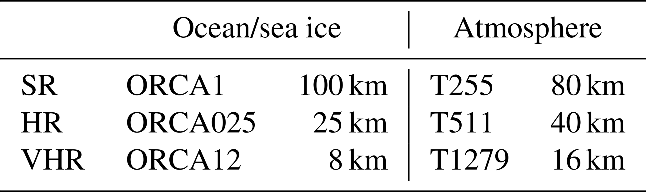
Table 1 Ocean and atmospheric grid configuration of each model resolution and the approximate resolution in mid-latitudes.

The HighResMIP protocol sets a minimum duration of 100 years for the 1950-control experiment (Haarsma et al., 2016). Although the lower-resolution experiments extend much longer, due to the high computational costs of the VHR version, the corresponding 1950-control could be run for only a total of 106 years. Therefore, the VHR experiment limits the number of years we consider for all the model configurations, as we prefer to keep comparable setups. Moreover, we discard the first 30 years of all simulations to avoid the effects of a drift that lingers after the relatively short spin-up period. The 50 years recommended by the HighResMIP protocol are insufficient for the model to reach a trend-free state on the ocean surface (Moreno-Chamarro et al., 2025). We therefore analyse 76 years of each simulation. Also, for all the experiments, we use a second-order polynomial detrending to remove residual model drifts that all the models preserve in the deep ocean layers (not shown).

2.2 Observational data

We use oceanic temperature and salinity observations to compare the vertical density profiles and MLD variability. In particular, we use the EN.4.2.2 g10 (EN4; Good et al., 2013) version based on Gouretski and Cheng (2020) mechanical bathythermograph and Gouretski and Reseghetti (2010) expendable bathythermograph corrections. To produce variables that are comparable for both experiments and observations, we compute in both cases the sigma0 and sigma2 potential density anomalies from monthly means of potential temperature and practical salinity using the TEOS-10 equation (Roquet et al., 2015). Then, we use the monthly sigma0 outputs thus derived to compute the MLD following the density threshold of 0.03 kg m⁻³, setting the reference depth at 10 m (de Boyer Montégut et al., 2004). In addition, to maximise comparability with the simulations, we select different time ranges in the observations, depending on the target analysis. We take the 21 years centred around 1950 (1940–1960) to compute all climatological values to stay close to the 1950 radiative forcing conditions. When assessing variability (e.g. with standard deviations and correlations), we instead consider the last 76 years available (1948–2023) so that both observations and simulations cover comparable timescales. Because observations include forced signals, which are not present in the simulations, a second-order polynomial is previously removed from the data to focus on the interannual variations, which are mostly internally driven. Sea ice concentration has been taken from the March 1940–1960 average from HadISST2 (Titchner and Rayner, 2014).

2.3 Meridional overturning streamfunction

To characterise the AMOC, we compute the meridional overturning streamfunction for the Atlantic basin in the native grid's y axis. Note that ORCA grids are almost regular in the 90° S–45° N range, which means that the computed transport at those latitudes will be virtually meridional. We define the transport as the cumulative sum, from bottom to top, of the return flow; see Eq. (1).

$$\begin{array}{}\text{(1)}& {\displaystyle }{\displaystyle }{\mathit{\psi }}_z(t,y,z)=-\underset{z^{\prime }=-H}{\overset{z}{\int }}\underset{x^{\prime }=x_{\mathrm{W}}}{\overset{x_{\mathrm{E}}}{\int }}v(t,x^{\prime },y,z^{\prime })\mathrm{d}{x}^{\prime }\mathrm{d}{z}^{\prime }\end{array}$$

Here, x_W and x_E are the west and east boundaries of the basin, respectively, and H is the basin depth.

In the subpolar region, the density profile changes sharply in the longitudinal direction due to the multiple processes occurring in the area (e.g. Arctic outflows, deep convection, western boundary current, subpolar gyre circulation). For this reason, we also analyse the overturning streamfunction in sigma-space (see Eq. 2), which is more suitable to capture the contributions from deep water formation in the subpolar North Atlantic region (Zhang, 2010; Foukal and Chafik, 2024):

$$\begin{array}{}\text{(2)}& {\displaystyle }{\displaystyle }{\mathit{\psi }}_{\mathit{\sigma }}(t,y,\mathit{\sigma })=-\underset{x^{\prime }=x_{\mathrm{W}}}{\overset{x_{\mathrm{E}}}{\int }}\underset{z^{\prime }=z_{{\mathit{\sigma }}_{\text{max}}}}{\overset{z_{\mathit{\sigma }}}{\int }}v(t,x^{\prime },y,z^{\prime })\mathrm{d}{z}^{\prime }\mathrm{d}{x}^{\prime },\end{array}$$

where $z_{{\mathit{\sigma }}_{\text{max}}}$ is the depth at which σ is maximum; in a stable ocean, this will be −H, as in Eq. (1). z_σ is the depth at which the density is equal to σ. Note that while integrals can be rearranged in Eq. (1), in Eq. (2), the integral in z^′ should be done first, as there is a change in the system of reference.

To study the AMOC signal driven by thermohaline changes in vertical ocean mixing, we remove the Ekman transport from the overturning streamfunction. We compute the total Ekman transport as the west-east integral of the surface wind stress divided by the Coriolis parameter and the reference density; see Eq. (3). Note that, as the net transport should be equal to 0, the resulting transport V in the Ekman layer (approximately the first 30 m) should be compensated by an equal and opposite transport, which is assumed to happen uniformly throughout the whole water column.

$$\begin{array}{}\text{(3)}& {\displaystyle }{\displaystyle }V(t,x^{\prime },y)=-{\displaystyle \frac{\mathrm{1}}{{\mathit{\rho }}_{\mathrm{0}}}}\underset{x^{\prime }=x_{\mathrm{W}}}{\overset{x_{\mathrm{E}}}{\int }}{\displaystyle \frac{\mathrm{1}}{f(x^{\prime },y)}}{\mathit{\tau }}_x(t,x^{\prime },y)\end{array}$$

Here, ${\mathit{\rho }}_{\mathrm{0}}=\mathrm{1025}\mathrm{kg}{\mathrm{m}}^{-\mathrm{3}}$ is the reference density, f is the Coriolis parameter, and τ_x is the zonal wind stress. The transport should be divided by the cross-section x–z area to recover the average speed, which is integrated as in Eqs. (1)–(2) to get the streamfunction in both the z and sigma spaces.

2.4 Result evaluation

All the scientific analyses are performed using well-established open-source scientific programming languages and tools. Most of the analyses are performed directly with Python and ESMValTool v2.11.0 (Righi et al., 2020; Andela et al., 2024a, b), a software package specifically created to facilitate a rigorous evaluation of CMIP simulation outputs that is especially useful for comparing multiple models with observational datasets.

We use Pearson's correlation coefficient, r, to assess the interrelation between variables in several analyses. The effective number of degrees of freedom, N_eff, of a correlation of N-length series is computed using the approach proposed by Afyouni et al. (2019) to take into account the temporal autocorrelation of the data; see Eq. (4).

$$\begin{array}{}\text{(4)}& {\displaystyle }{\displaystyle }{N}_{\text{eff}}=N{\left(\mathrm{1}+\mathrm{2}\sum _{k=\mathrm{1}}^{N-\mathrm{1}}{\displaystyle \frac{N-k}{N}}{r}_{XX,k}{r}_{YY,k}\right)}^{-\mathrm{1}}\end{array}$$

Here, r_XX,k and r_YY,k are the autocorrelations of each series at lag k. Their statistical significance is computed according to a Student's t distribution setting a p value of 0.05 (i.e. 95 % confidence level) to determine if the correlation is statistically different from 0.

3 Results

3.1 North Atlantic mixing

We first look at the climatology of the MLD in March, the month in which it reaches its yearly maximum. In the three model versions (Fig. 1a–c), the Labrador and Irminger seas appear to have a stronger mixing than the Nordic Seas (Fig. A1 shows the locations of all geographical regions referenced in the results). The models show qualitative and quantitative differences with each other in the areas with active mixing around the Labrador Sea. The MLD in the subpolar gyre is much more intense in HR (Fig. 1b), where it exceeds 2000 m in a broad region covering both the Irminger and Labrador seas. By contrast, VHR (Fig. 1c) has a thinner mixed layer climatology, which can locally reach up to 1500 m deep in the Labrador Sea interior. In addition, VHR has a comparatively shallower mixing south of Cape Farewell and the Irminger Sea. SR (Fig. 1a) shows an even smaller MLD of about 1000 m, concentrated in a small region south of Cape Farewell. This model configuration has, in fact, a positive bias in the sea ice concentration covering the western Labrador Sea (see the contour lines in Fig. 1), which dampens the local air–sea interactions and, subsequently, the mixing. For similar reasons, due to the positive bias in sea ice concentrations in the Nordic Seas, all the model configurations simulate very little mixing in that region.

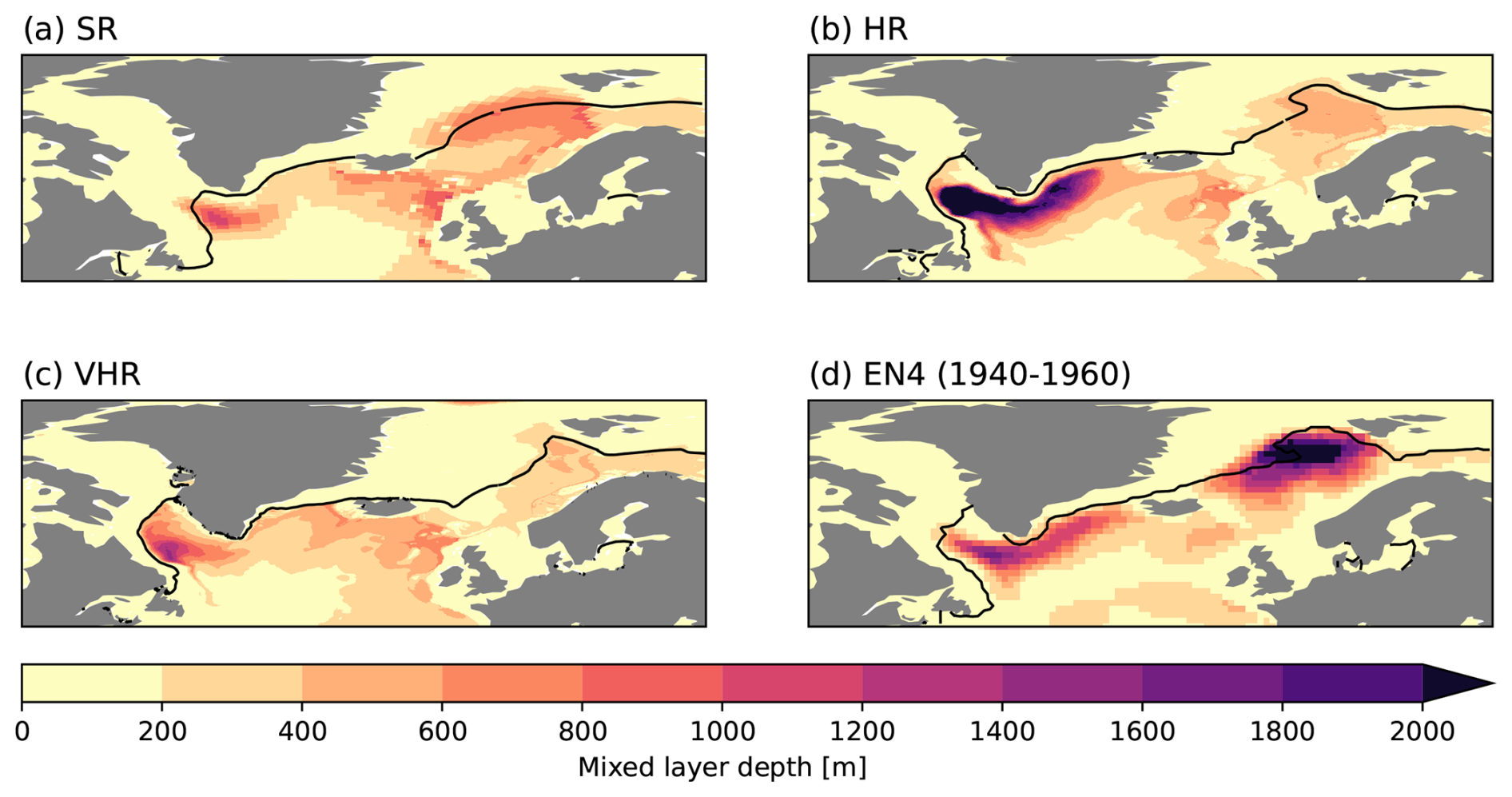
Figure 1 March MLD climatology for SR (a), HR (b), VHR (c), and EN4 1940–1960 (d). The black contour line shows the climatological March sea ice concentration at 15 % for the same dataset in (a–c) and for HadISST2 1940–1960 in (d).

By contrast, EN4 (Fig. 1d) shows very intense mixing in the Nordic Seas region, with much stronger values than in the models, which can locally exceed 2000 m in depth. Some of these differences, however, might derive from the large uncertainties in EN4 during the considered period (1940–1960), in which observations in the subsurface were very scarce (Killick, 2021). It could also happen that the way of generating this observation-based product affected the estimated MLD values. EN4 uses spatial and temporal interpolations of different observational sources, including instantaneous profiles, to produce a monthly regularly gridded dataset. This process may artificially reduce the vertical stratification, resulting in a higher MLD (de Boyer Montégut et al., 2004). Nonetheless, EN4 still gives useful qualitative information about the spatial extent and the key regions of deep water mixing, allowing us to conclude that all model configurations underestimate the mixing in the Norwegian Sea, with values that are consistently shallower than in the Labrador Sea, unlike in observations.

When looking at the variability of the MLD, as represented by the standard deviation in time, this is generally greater in the regions where the climatological mean values are also large (Fig. 2). In the case of SR and HR, Fig. 2a and b, the standard deviation in the western subpolar gyre is of similar magnitude, reaching maximum values of around 1000 m, although differences are found in the Nordic Seas, where SR shows higher variability. Compared to SR and HR, VHR shows lower variability in the Labrador Sea, with values of around 400 m and even lower in the Nordic Seas (Fig. 2c). In EN4, for the 1948–2023 period (Fig. 2d), we see consistently stronger variability than in the models (i.e. values above 1300 m) in all regions. The substantially higher observational uncertainty in the early part of EN4 compared to the present period may affect the associated MLD variability. We also note that EN4-derived data might include forced signals that have not been properly removed by the polynomial detrending. These include low-frequency modulations not present in the (unforced) control simulations, as well as some additional interannual variability linked to the response to the three major volcanic eruptions that occurred in 1963, 1982, and 1991.

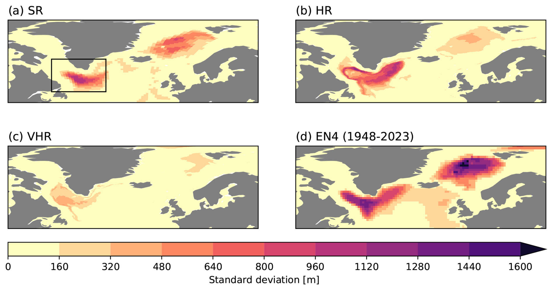
Figure 2 March standard deviation of MLD for SR (a), HR (b), VHR (c), and EN4 1948–2023 (d). The box used to compute MLD time series and vertical profiles is shown in (a).

We now focus on the Labrador Sea, where the models show important MLD differences and where MLD has extensively been linked to changes in the AMOC (Koenigk et al., 2021; Ortega et al., 2021; Yeager et al., 2021; Lin et al., 2023). To understand the differences in the MLD mean state and variability across the three model configurations and observations, we examine their vertical density stratification, which is a key preconditioner for mixing. Figure 3a shows the climatological vertical profiles of density in March for the Labrador Sea, computed as area-weighted averages in the box 60–35° W 50–65° N (from Ortega et al., 2021), also shown with a black box in Fig. 2a. The Labrador Sea density is found to be more stratified in SR than in EN4 and less stratified in HR and VHR. We use two different complementary metrics to measure the degree of agreement of the simulations with the observed profile, namely, the root-mean-square-error (RMSE) and the correlation, both estimated in the vertical dimension. SR is the model configuration with the best agreement with EN4 in terms of RMSE, while VHR has the best agreement in terms of correlation, followed closely by SR (Table 2). Overall, HR shows the poorest agreement with EN4, and it is also the model configuration that represents the weakest vertical stratification, which can explain why its MLD climatology is overly strong, as the threshold it has to overcome is smaller. This can also be seen in Fig. 3d, which shows the linear regression coefficients of the MLD time series with the vertical density profile, as an additional diagnostic to compare the models with the observations. The density anomaly needed in the top ocean to generate one metre of MLD is much smaller in HR compared to the other two model configurations, although, interestingly, it stays closer to the observed regressed value. Somehow, surprisingly, the largest differences with respect to the observed regressions happen for VHR, which had the most realistic climatological profile.

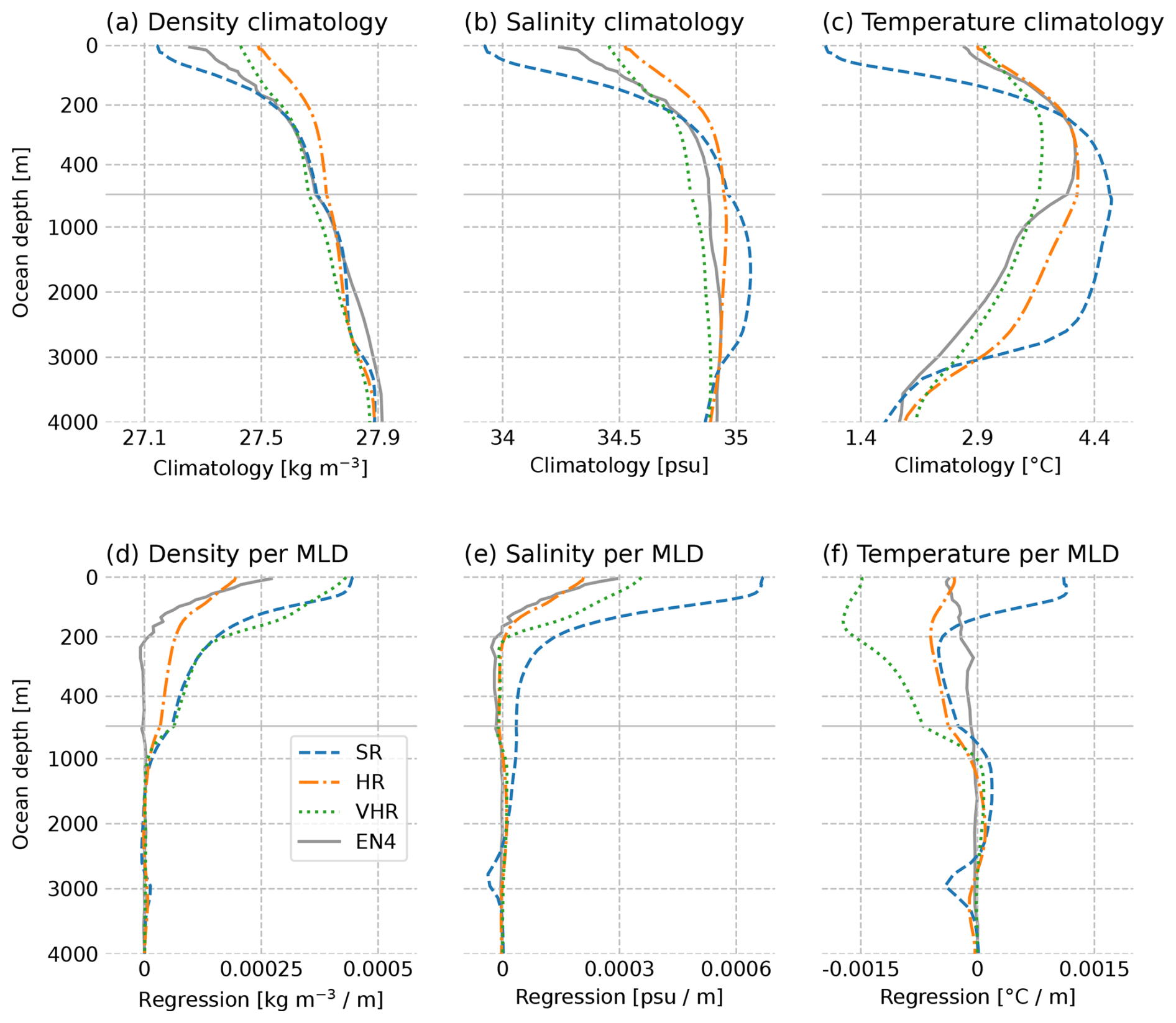
Figure 3 March vertical profiles for SR, HR, VHR, and EN4 1948–2023 in the Labrador Sea box (from Fig. 2). The first row shows the sigma0 density (a), salinity (b), and temperature (c) climatologies. The second row shows the sigma0 density (d), salinity (e), and temperature (f) regression coefficients with the March Labrador Sea MLD time series. The horizontal grey line divides the upper 500 m, where data have been enlarged, from the lower 500 m.

Table 2 Correlation (corr) and root-mean-square error (RMSE) of the climatological vertical profiles from Fig. 3a–c of three model configurations with respect to EN4. All the correlations are significant, with a p value $\ll \mathrm{0.05}.$ Results with the best performance, i.e. higher correlation and lower root-mean-square error, are highlighted in bold.

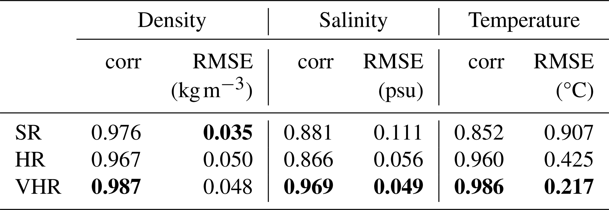
To gain further insights, the analysis is expanded to the temperature and salinity profiles. Even if the vertical density profile may suggest that SR is the model configuration in best agreement with the observational dataset near the surface, we can see that it happens for the wrong reasons, as there is a strong error compensation between the biases in the salinity (Fig. 3b) and temperature (Fig. 3c). When looking at those variables, VHR is consistently the model configuration in best agreement with EN4 regarding both temperature and salinity profiles, also reflected in the correlation coefficients and RMSEs shown in Table 2. Interestingly, for all three model configurations, the density profile is clearly dominated by salinity, as inferred by the vertical profiles of the haline and thermal contributions to the Labrador Sea densities (Fig. A2), in which temperature has a minor influence and opposes the contribution from salinity. The better representation of the vertical profile in VHR may be due to several factors. Although VHR does not have the resolution required to explicitly resolve eddies in the Labrador Sea (a resolution of $\mathrm{1}/\mathrm{16}$° would be necessary; Hallberg, 2013), it has a fine-enough resolution to do so in the Gulf Stream and the North Atlantic Current. These currents play a key role in transporting heat and salinity to northern latitudes, which can improve the climatological conditions in the subpolar gyre, including in the Labrador Sea. Additionally, better topography, improved resolution of boundary currents, and enhanced air–sea interaction, among other processes, may also contribute to correcting these biases.

Salinity regressions against MLD time series show that, overall, HR has the best agreement with EN4 (see Fig. 3e), with VHR being the second best, with overly salty regression values in the upper ocean. By contrast, SR overestimates the regression values at the surface by a factor of 2, which might be related to the large negative bias in the corresponding climatological profile (Fig. 3b). The temperature regression against the MLD shows the largest qualitative discrepancies between models and observations (Fig. 3f). While observations show a moderate negative link between the mixing and local temperatures that is maximum at the surface and decreases monotonically with depth, both HR and VHR do show a negative link, but stronger in the subsurface (∼200 m). It is also worth noting that regression values for VHR are almost 1 order of magnitude higher than for HR and the observations. However, the largest discrepancies with respect to EN4 occur for SR, for which the regression values near the surface are of the opposite sign (i.e. positive instead of negative). This change in sign can be explained by the particularly strong local bias in sea ice, which is associated with both cold ocean conditions and reduced mixing. The inter-model differences revealed by the regression patterns for the mixed layer depth point to potential differences in the drivers of Labrador Sea mixing, which are investigated in the following.

3.2 Drivers of deep water mixing variability in the Labrador Sea

We first compare the local atmospheric forcing exerted by the zonal wind across resolutions, which in winter generally brings cold air masses from the continent. Figure 4a–c shows the correlation in time between December–March (DJFM) wind stress in the x-grid direction (zonal in mid-latitudes) over the North Atlantic and the time series of the Labrador Sea MLD in March. All the model configurations show a dipole-like pattern, with some qualitative and quantitative differences. In the HR and VHR configurations, the pattern shows a strong positive correlation band going from approximately 40 to 65° N and a negative correlation band south of 40° N. This dipolar wind structure has typically been associated with a positive North Atlantic Oscillation (NAO) phase (e.g. Ortega et al., 2012) and also matches the one from the first EOF of the zonal wind stress (not shown). This means that, for both experiments, positive NAO phases tend to increase the mixing, while negative NAO phases tend to reduce it, as already shown in other studies (Ortega et al., 2021; Patrizio et al., 2023). To corroborate this, Fig. 4a–c also includes (in contours) the correlation of Labrador Sea MLD in March with the mean sea level pressure in DJFM, which shows a clear NAO-like dipole, with positive correlations over the Azores High and negative correlations over the Icelandic Low. Following the increase in the zonal wind, both HR and VHR show a cooling of the surface water masses through enhanced heat loss to the atmosphere (Fig. 4e and f), which makes them denser and thus promotes local mixing as shown by Kostov et al. (2019). In the case of SR, we observe a similar pattern for the wind stress to that in HR and VHR, but with weaker correlation coefficients that are also more confined to the basin's western side. The weaker correlations for the wind also result in weaker correlations for the surface heat fluxes, which are not significant in the western part of the Labrador Sea, where the presence of sea ice precludes the local interactions with the atmosphere on the western side of the sea. This results in the impact of the NAO being less strong and widespread as for the other two model configurations. In all cases, the impact of atmospheric forcing through the zonal wind stress happens on a year-to-year scale. The next considered driver is associated with longer-time-scale advective processes.

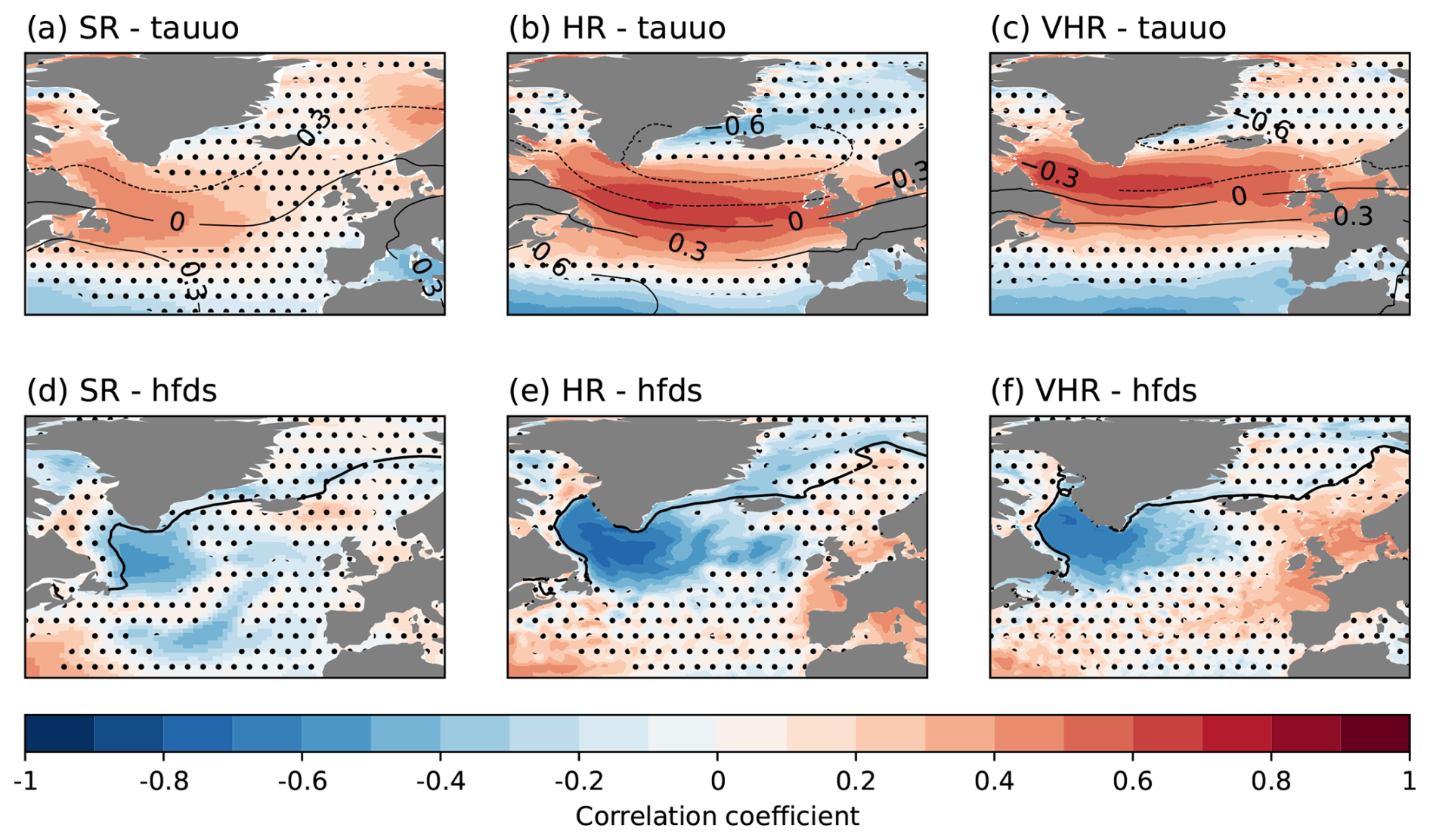
Figure 4 (a–c) Correlation of the Labrador Sea MLD in March with the DJFM eastward wind stress (colours) and the DJFM sea level pressure (contour lines) over the North Atlantic for SR, HR, and VHR, respectively. Non-significant values are masked with dots to improve the visibility over the significant areas. (d–f) The same but between the Labrador Sea MLD in March and the DJFM surface downward heat fluxes. In these three panels, the thick black contour line shows the climatological line of 15 % sea ice concentrations in March.

At all three model configurations, salinity has been shown to have an important role in explaining the surface density profiles as well as the changes in the MLD in the Labrador Sea. We will now explore the origin of those salinity signals and how they are linked to changes in the mixing by computing correlations between the annual surface salinity fields and the March MLD index in the Labrador Sea (Fig. 5). When both variables are in phase, that is, at lag 0, all three experiments show strong positive correlations with salinity in the Irminger and the eastern Labrador seas, extending farther east in SR and HR, and westward into the Labrador Sea in VHR (Fig. 5j–l).

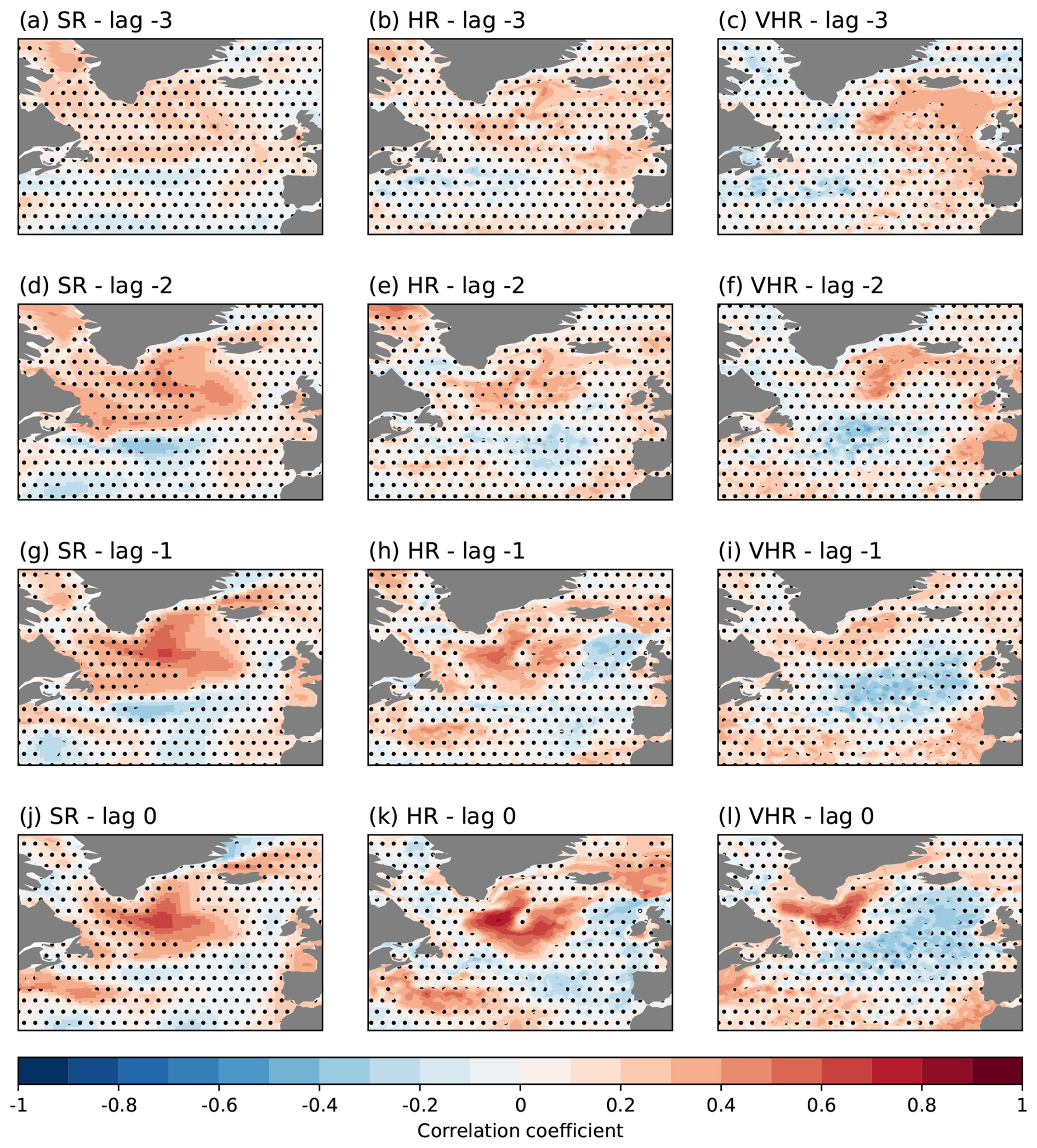
Figure 5 Correlation of March Labrador Sea MLD with yearly surface salinity for SR (a, d, g, j), HR (b, e, h, k), and VHR (c, f, i, l); lagged 3 years (a–c), lagged 2 years (d–f), lagged 1 year (g–i), and no lag (j–l). Non-significant values are masked with dots to improve the visibility over the significant areas.

The subsequent lagged correlations allow us to track down the origin of the surface salinity signals. When lagging the MLD by 1 year (Fig. 5g–i), SR and HR still show positive significant correlations in the same area, which suggests that they build up over the years, probably due to positive feedback linked to the local salinity stratification conditions. VHR no longer shows significant correlations in the Labrador Sea, but it does a bit further north near the Irminger Sea, where the other two model configurations also show slightly higher correlation values than at lag 0, which suggests some salinity propagation. When the MLD index lags by 2 years (Fig. 5d–f), the three experiments show a positive significant correlation in the northeastern part of the Irminger Sea, south of the Denmark Strait, further supporting the aforementioned propagation. Likewise, when the MLD index lags by 3 years (Fig. 5a–c), we still see significant correlations in the same area for HR, and in the case of VHR, the area of significant correlations is displaced to the east, extending from Iceland all the way to the British Islands. By contrast, no significant correlations are found for SR in those regions. The propagation of salinity anomalies, more evident in VHR, is probably explained by the mean transport of the subpolar gyre circulation. Similar correlation patterns have been produced against the surface temperature fields (Fig. A3), but they do not show any clear advection of temperature signals into the Labrador Sea for any experiment, which excludes temperature propagation as a key driver of Labrador Sea mixing.

Our results so far have shown differences across the three model configurations of EC-Earth3P in terms of vertical mixing, preconditioners, and drivers of its variability, which could result in major differences regarding their link with the ocean circulation. In the next section, we will therefore study this link with the AMOC.

3.3 Impact of resolution in the variability and meridional coherence of the Atlantic Meridional Overturning Circulation

The mean state of the AMOC also varies with resolution. All analyses in this section are based on the volume streamfunction in density space, which is more adequate to represent the contributions of deep water formation in the subpolar North Atlantic than in depth space (Zhang, 2010; Foukal and Chafik, 2024). Furthermore, the Ekman transport has been removed from the volume streamfunction to focus on its thermohaline component, which is more directly linked to the vertical mixing. When computing the volume overturning streamfunction without the Ekman transport in sigma2 space, all the models show the maximum value of the climatology around 55° N and 36.8 kg m⁻³ (Fig. 6, contour lines) but with different magnitudes. HR and VHR show the strongest AMOC, with values greater than 20 Sv in both cases, although slightly higher in HR. Meanwhile, in SR, the highest value is lower than 20 Sv. The three model configurations have the strongest variability of the AMOC situated at the same latitude as the maximum but at a slightly higher density level (Fig. A4). Interestingly, despite having the weakest mean AMOC state of the three experiments, SR shows higher variability than the rest, with HR and VHR exhibiting similar values. Therefore, the AMOC mean state and variability are largely comparable between HR and VHR but differ in SR.

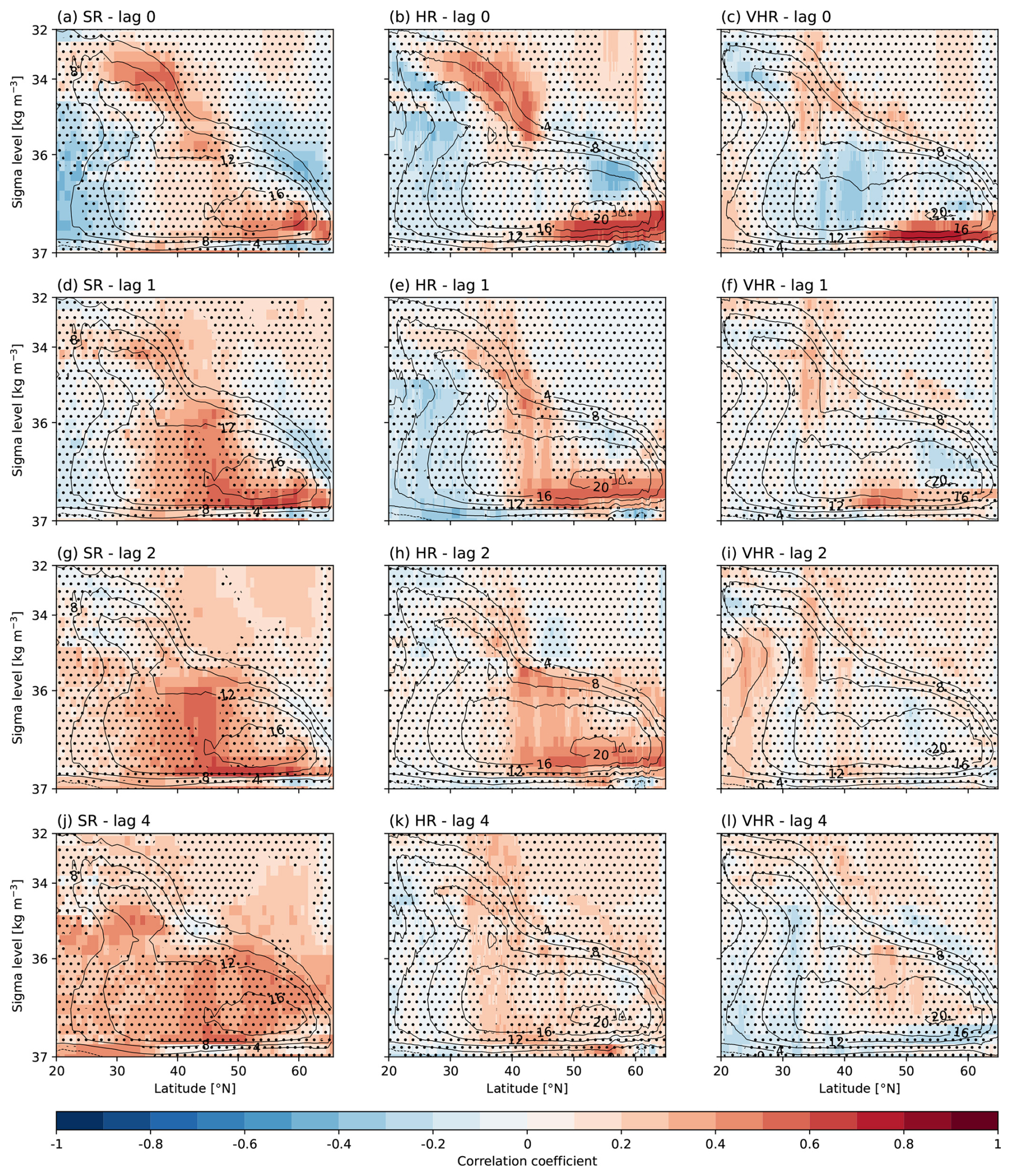
Figure 6 Correlation of March Labrador Sea MLD with yearly averaged volume overturning streamfunction without the Ekman transport in sigma2 space for SR (a, d, g, j), HR (b, e, h, k), and VHR (c, f, i, l); streamfunction with no lag (a–c), lagged 1 year (d–f), lagged 2 years (g–i), and lagged 4 years (j–l). Non-significant values are masked with dots to improve the visibility over the significant areas. Contour lines show the climatologic volume overturning streamfunction without the Ekman transport in sigma2 space.

Newly formed dense waters in the Labrador Sea are usually propagated southward along the DWBC (Ortega et al., 2021). As these dense waters resulting from the vertical mixing move southward, they change the zonal density gradient, triggering a thermal wind balance response that leads to a general intensification of the AMOC. To explore whether this link is affected by resolution, Fig. 6 compares the response of the AMOC to changes in the Labrador Sea MLD in March across the three model configurations, using lagged correlations in which the Labrador Sea mixing always leads the AMOC. For the SR model, the lagged correlations of the overturning streamfunction in density space with the MLD show how, over lead times from 0 to 4 years, the significant correlations at the densest levels (≥36.7 kg m⁻³, i.e. those formed by the deep mixing) progressively move southward, reaching 20° N. However, the propagation pattern is different at finer resolutions. At lag 0, HR and VHR show much stronger correlations than SR in the subpolar latitudes (i.e. north of 45° N), where deep water mixing occurs. The main differences between HR and VHR emerge at subsequent lead times, when significant correlations progressively reach more southern latitudes, in line with a southward propagation of the AMOC signals. In the case of HR, a very slow propagation is hinted, with the area of significant correlations reaching the 35° N latitude by the fourth lead year. Meanwhile, VHR shows a very quick drop of the correlation values already in the first lead year, with significant correlations limited to the 40–50° N latitudinal band. Interestingly, at lag 2, we observe a wide range of densities (i.e. 35–37 kg m⁻³) showing significant correlations south of 25° N, although the lack of coherence with the previous subpolar signals raises the question of whether they have propagated from the subpolar region, represent a local response, or are simply a spurious correlation.

The southward propagation of the AMOC response to changes in the Labrador Sea deep mixing can be better captured if the density level is fixed, as this allows the temporal evolution to be visualised in a single plot. Figure 7a–c shows the correlation of Labrador Sea MLD in March with the annual AMOC at the 36.73 kg m⁻³ sigma2 level, as a function of lead time with MLD leading. The largest correlations between AMOC and MLD happen at lag 0 and between 50 and 65° N. Subsequent lead times show how the significant positive correlations move southward, although with notable differences across resolutions regarding the timescales and the southward extent of the AMOC propagation. The SR shows a relatively slow propagation to about 45° N in about 2 to 3 years, with correlations becoming insignificant beyond that lead time and latitude. This slow propagation appears to be consistent with the advective propagation regime described by Zhang (2010), although they found it to reach 34° N. The propagation in HR shows two distinct timescales; there is a fast propagation within the first year to approximately 40° N, followed by a much slower one that reaches 35° N over 8 years. The fast one could be linked to fast wave propagation, as enhancing resolution enables the representation of boundary waves, such as Kelvin waves (Getzlaff et al., 2005). Even if the propagation pattern found in HR does not match the one described by Zhang (2010), it is consistent with recent results by Kostov et al. (2023). In the VHR model case, a much weaker cross-latitudinal link between the MLD and the AMOC is seen. Only a fast propagation such as the one seen in HR occurs in this experiment, although with weaker correlations that also remain significant for a shorter period.

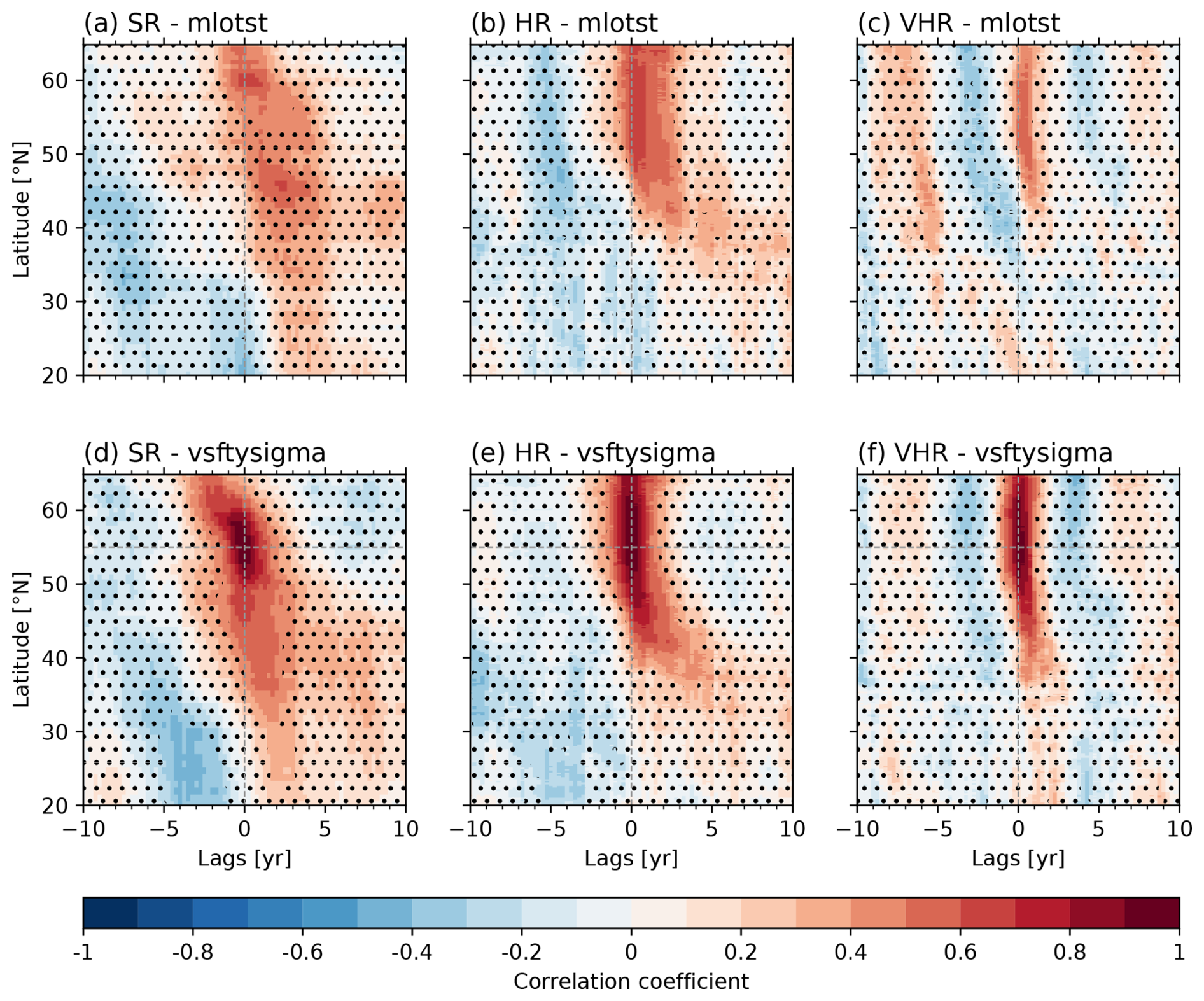
Figure 7 Correlation of the monthly volume overturning streamfunction without the Ekman transport at the 36.73 kg m⁻³ sigma2 density level with March Labrador Sea MLD (a–c) and with itself at 55° N (d–f) for SR (a, d), HR (b, e), and VHR (c, f). For positive lags, the March Labrador Sea MLD (a–c) or AMOC at 55° N (d–f) leads. Non-significant values are masked with dots to improve the visibility over the significant areas.

To further inspect the cross-latitudinal coherence of AMOC changes, which might not be necessarily driven by changes in the Labrador Sea mixed layer, we have recomputed the same lagged correlations but between the AMOC fixed at 55° N (where it exhibits the strongest climatological values) and the basin-wide AMOC streamfunction, both defined again at the 36.73 kg m⁻³ sigma2 level (Fig. 7d–f). As expected, this version has systematically higher correlation values than the previous one, which helps to better illustrate the gradual southward propagation of the AMOC changes. For SR, we now see that the subpolar AMOC is connected with the AMOC at 20° N with a delay of 2–3 years. For HR, the main results are very similar to those previously described for the correlations with the mixing, with a very clear fast propagation from the northern latitudes to 45° N, followed by a slowly paced propagation to 30° N over the next 6 years. In VHR, we can now see that the strength of the correlations is comparable to that in HR and SR, in contrast with the correlations against the mixing. We also note for VHR an almost continuous band of significant correlations from the subpolar to the tropical latitudes, with a 1–2 year lag between 55–37° N and an almost instantaneous connection between 35–20° N. This plot suggests that, for VHR, other influences than the Labrador Sea mixing are responsible for the southward propagation of AMOC changes, which is consistent with some recent studies suggesting that Labrador Sea water formation may not be a crucial driver of AMOC (Lozier et al., 2019; Zhang and Thomas, 2021).

The lagged correlations of the large-scale density field with the Labrador Sea MLD index give further information on how the signal produced by the mixing propagates along the western boundary, subsequently impacting the AMOC (Fig. 8). For each grid point, we extract the maximum correlation in the depth range from 400 to 1400 m, which is where the highest change in density related to mixing happens (Fig. A5). To better examine the structure of the boundary current, we also computed the lagged correlations between the Labrador Sea MLD index and the ocean densities along a zonal cross-section located at 45° N off the coast of Newfoundland (Fig. A6). Other cross-sections have also been considered, yielding similar results (not shown). At lag 0, all simulations show significant positive correlations in the interior Labrador Sea but with differences across model configurations in their location (more central in SR, flanked to the east in HR, and to the west in VHR). Inter-model differences are also found along the boundary currents. In SR, only the Greenland Current shows clear and significant correlations, and in HR, significant values (stronger than for the Labrador Sea interior) extend from the Greenland Current to the Labrador Current and around the Grand Banks area down to 40° N, remaining significant until Cape Hatteras. In VHR, a distinct band of significant correlations extends from the Labrador Current all the way to Florida (∼30° N). These results thus describe a very rapid (subyearly) propagation occurring both at HR and VHR, with the final latitude reached likely determined by the location where density anomalies in the interior Labrador Sea are formed. In VHR, significant correlations are also found further south, but they are stronger and span a much wider zonal extent, suggesting that they originate from a different process than the boundary propagation (e.g. a wind effect not accounted for when Ekman transport is removed).

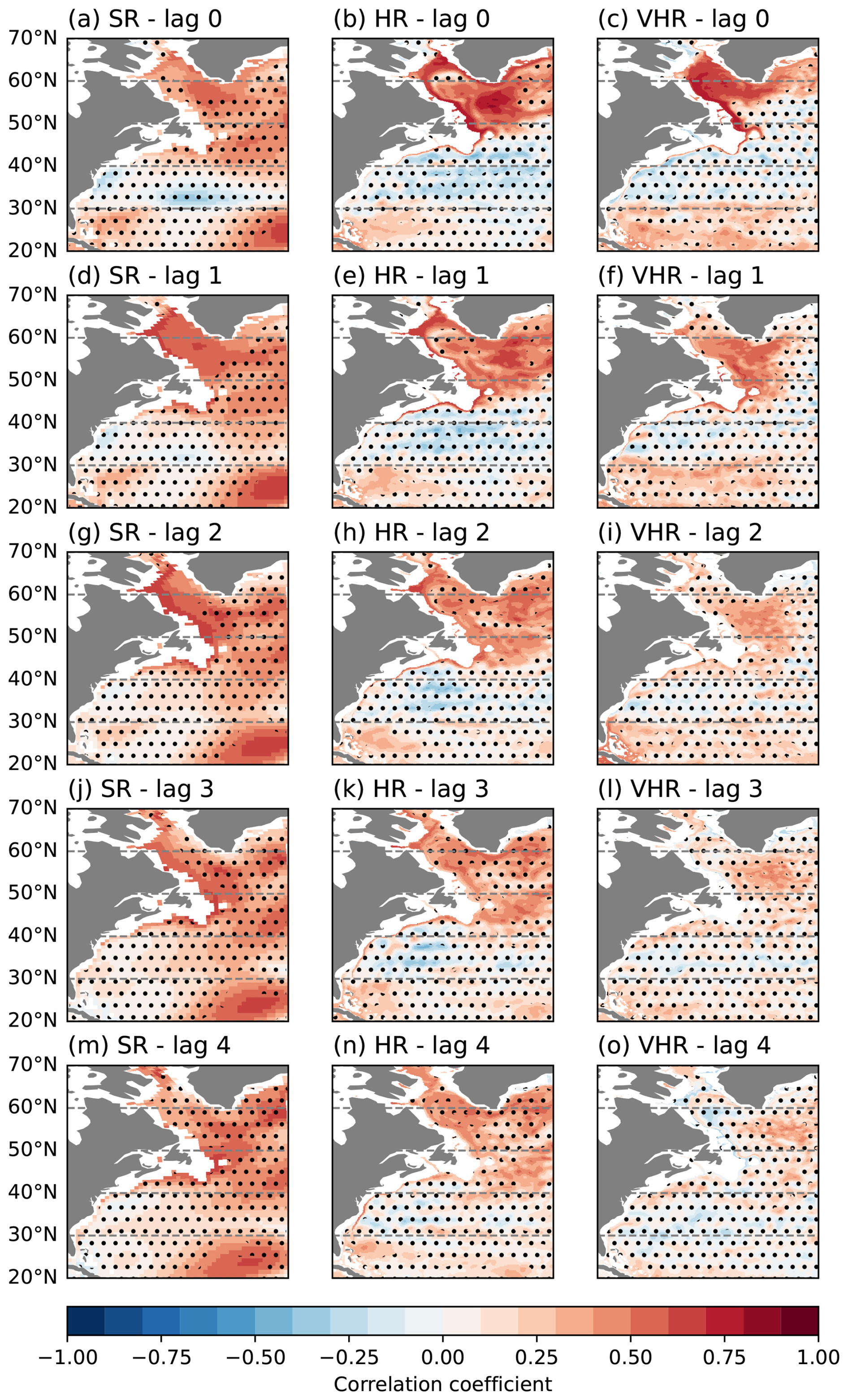
Figure 8 Maximum correlation between the Labrador Sea MLD index and the yearly sigma2 density fields from 400 to 1400 m for SR (a, d, g, j, m), HR (b, e, h, k, n), and VHR (c, f, i, l, o); density with no lag (a–c), lagged 1 year (d–f), lagged 2 years (g–i), lagged 3 years (j–l), and lagged 4 years (m–o). Non-significant values are masked with dots to improve the visibility over the significant areas.

At subsequent lags, further differences across experiments are revealed. For SR, a slow propagation is hinted at, with significant correlations gradually reaching 40° N at lag 1, 35° N at lag 2, and 25° N at lag 3. As expected from the coarser grid spacing and higher viscosity in SR, the DWBC is also wider and more zonally coherent than at higher resolutions. However, significant correlations in SR tend to remain more constrained to the coast and occur at shallower levels than in HR and VHR (Fig. A6). For HR, correlations remain significant along the boundary at all lags considered, reaching the southernmost tip of Florida at lag 3. This contrasts with the results of VHR, for which significant correlations are no longer found along the boundary by lag 3. The greater persistence of significant correlations in HR, along with the gradual southward displacement of the latitudes with the strongest correlation values, is consistent with the slow propagation of AMOC signals found for this simulation in Fig. 7.

4 Discussion and conclusions

This paper explores whether and how the simulated mixed layer depth (MLD) in the subpolar North Atlantic, as well as its main drivers and links with the Atlantic Meridional Overturning Circulation (AMOC), are affected by horizontal resolution. For that, we use HighResMIP 1950-control experiments at three different resolutions of the coupled global model EC-Earth3P, i.e. an eddy-parameterised version (1° in the ocean mid-latitudes; SR), an eddy-present one (0.25° in the ocean mid-latitudes; HR), and an eddy-rich one ($\mathrm{1}/\mathrm{12}$° in the ocean mid-latitudes; VHR), all of which were developed during the PRIMAVERA project and following the HighResMIP protocol (Moreno-Chamarro et al., 2025).

Important differences between the different resolutions have been found. The main findings of our study are summarised as follows:

• The Labrador Sea is the Northern Hemisphere region with the deepest mixed layer in all model versions, with VHR's climatological values showing the best agreement with EN4 observations both in terms of magnitude and spatial extent. HR largely overestimates the Labrador Sea MLD, and SR underestimates it, an underestimation that is connected to a negative sea ice bias in that model configuration. None of the configurations, however, show ocean deep mixing in the Nordic Seas, as found in the observations, which can be linked to an excess of regional sea ice.

• The more realistic climatological value of the Labrador Sea MLD in VHR is consistent with an improved representation of the local stratification with respect to the other two experiments. In particular, the vertical temperature and salinity profiles are better represented.

• The atmospheric forcing on the Labrador Sea mixed layer depth is very similar in the VHR and HR configurations and is ultimately linked to the North Atlantic Oscillation (NAO). Positive NAO phases are found to enhance the Labrador Sea mixing, while negative NAO phases reduce the mixing there. In SR, the atmospheric forcing is weaker and more constrained to the basin's western side, which could be partly due to a shielding effect of the overly extended sea ice on the ocean.

• Surface salinity is also found to be an important contributor to the variability of the Labrador Sea mixing at all model configurations, facilitated by a positive feedback that enhances the persistence of the local salinity signals. Inter-model differences emerge regarding the origin of the surface salinity signals. In VHR, Labrador Sea mixing is preceded by a slow propagation of surface salinity signals from the eastern flank of the subpolar gyre into the Labrador Sea. Such a distant propagation is absent in both HR and SR.

• Labrador Sea MLD imprints on the AMOC show three distinct behaviours both in terms of latitudinal extension and time persistence of the AMOC changes. VHR shows an almost instantaneous response of the AMOC to the MLD changes in the Labrador Sea, a response that has limited latitudinal reach, extending up to only 37° N, and only persists for 1–2 years. Meanwhile, SR shows a more gradual and persisting response of similar latitudinal reach, and HR shows an initial rapid response down to 40° N, followed by a slow response that gradually reaches the tropics. An additional analysis of the AMOC's cross-latitudinal coherence shows a significant connection in VHR between the subpolar AMOC and the subtropics, not evidenced in the AMOC response to Labrador Sea MLD, which suggests the presence of other important drivers of AMOC variability.

• An analysis of the link between the Labrador Sea MLD and the densities across the deep western boundary current confirms a very fast propagation of Labrador Sea density signals along the boundary current in VHR, occurring within the first year and reaching 30° N. By contrast, SR shows a slow propagation pattern, with a boundary density signal reaching the tropics after 4 years. In HR, there is a combination of the fast and slow propagation of density anomalies observed respectively for VHR and SR. These boundary densities are expected to drive, through thermal wind balance, a latitudinally coherent AMOC response that reaches the subtropics. In VHR, however, the boundary signals are rather weak when they reach Cape Hatteras, which might explain why they are unable to generate an AMOC response in the subtropics.

These results show different behaviours for the ocean circulation and its driving processes in the North Atlantic across resolutions. Therefore, further research is needed to confirm if similar differences are identified in other climate models to thus determine if eddy-resolving models consistently bring new regimes of variability that could challenge our current understanding of the future changes to be experienced by the AMOC, which predominantly come from models with eddy-parameterised oceans.

This study investigated the differences in the mixed layer depth, its drivers, and its impact on the AMOC across resolutions. It therefore makes sense to discuss how well every experiment compares to observations, as a way to elucidate if VHR is actually more realistic, thus justifying its substantially higher computing costs to carry on similar studies. However, the comparison to observations was hindered by different factors. The most important factor is that our simulations correspond to a period of fixed 1950 radiative forcing conditions, while observations describe an evolution that was shaped by transient radiative forcings. Also, the availability and quality of oceanic observations near the year 1950 are very limited, particularly for the subsurface. Indeed, the number of observations has dramatically increased in the last 30 years (Gould et al., 2013), thanks to the deployment of satellites, the launch of in situ measurement projects like Argo (started 20 years ago; Roemmich et al., 2009), and transport-measuring arrays like RAPID (started 20 years ago; Moat, 2023) at 26° N and OSNAP (started 10 years ago; Fu et al., 2023) in the subpolar region. However, this period is substantially warmer than 1950 and thus not representative of its mean climate. For this reason, we limited our comparison with observations to variables and regions with reasonably good data coverage around the 1950s. Another major limitation related to the study of control experiments concerns the evaluation with observations of temporal features and covariances between variables, which include externally forced signals in the observations that may not be possible to remove with a polynomial detrender. Moreover, the limited time span of mass-transport observations from the OSNAP and RAPID arrays, along with the sparse spatial information they provide, substantially hinders our understanding of the real-world linkages between the mixed layer depth and the AMOC (Jackson et al., 2022; Frajka-Williams et al., 2023). This same problem hampers our knowledge of how coherently the AMOC changes across latitudes. Extending sustained AMOC measurements to other latitudes and improving the realism of ocean reanalyses for dynamical large-scale variables are therefore essential to fill that knowledge gap.

Multimodel analyses are also important for building confidence in the impact of model resolution and its potential added value, in particular for processes where observations are sparse. Results that are consistent across models are more likely to be reliable, whereas model-dependent results indicate higher uncertainty. In this sense, previous studies suggest that while our results might be model-dependent, others are consistent. Koenigk et al. (2021) explores the impact of resolution on the mixed layer depth and includes HadGEM3-GC31-HH, which shares the same ocean component (NEMO3.6) of EC-Earth3P-VHR configured at the same ocean resolution. However, the MLD from HadGEM3-GC31-HH is more comparable to our HR configuration than to VHR, also showing stronger convection in the Nordic Sea, which is underestimated in our experiments. AMOC latitudinal coherence (defined as the connection between the AMOC anomalies across latitudes) has been shown (in Fig. S1 in the Supplement of Roberts et al. (2020)) to vary across models and resolutions. The propagation pattern we find in VHR is similar to the one they show for HadGEM3-GC31-HH, which suggests that eddy-rich models have a weak AMOC coherency between subpolar and subtropical latitudes.

It is also important to consider that the 76 years considered in our analyses may be insufficient to sample the decadal and multidecadal variability and constrain accurately the statistical significance of the covariances explored. However, this is a problem that derives from the HighResMIP protocol itself, which considers 100-year control simulations as a compromise to assess internal variability at interannual scales while minimising the computational and data storage needs. Longer model integrations or multi-ensemble simulations are therefore desirable to improve our understanding of decadal variability, which might be more affordable by coordinating efforts between different modelling centres, such as is currently planned within the European project EERIE and the next phase of HighResMIP. More generally, these joint multi-model efforts are also important to shed new light on the key role played by mesoscale ocean eddies on the climate, including its future response to the projected greenhouse gas emissions.

Appendix A: Supplementary figures

$$\begin{array}{}\text{(A1)}& {\displaystyle }& {\displaystyle }\text{SigmaS}=b\left(S-\stackrel{\mathrm{‾}}{S}\right)\text{(A2)}& {\displaystyle }& {\displaystyle }\text{SigmaT}=-a\left(T-\stackrel{\mathrm{‾}}{T}\right)\text{(A3)}& {\displaystyle }& {\displaystyle }\text{Sigma}=\left(\text{sigma0}-\stackrel{\mathrm{‾}}{\text{sigma0}}\right)=\text{SigmaS}+\text{SigmaT}\end{array}$$

Here, a is the thermal expansion coefficient, and b is the haline contraction coefficient.

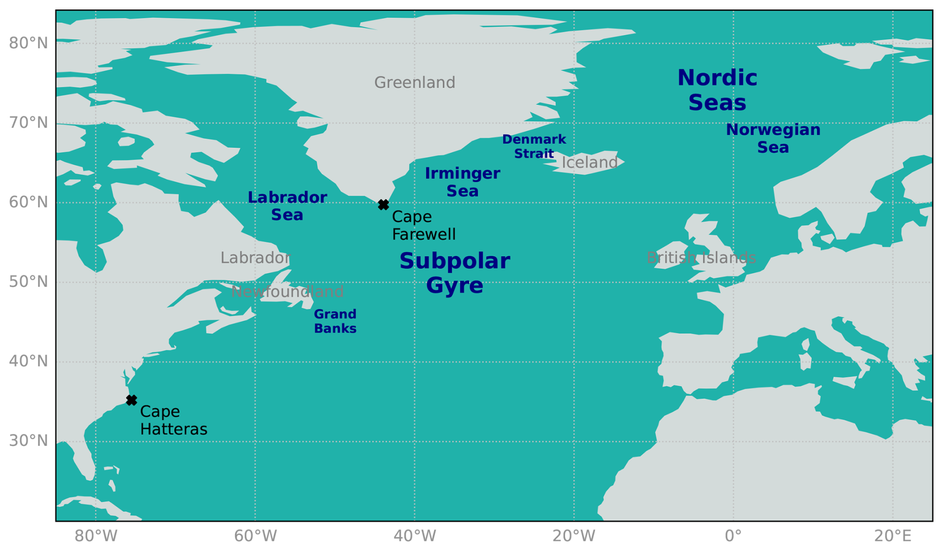
Figure A1 Map including geographical references.

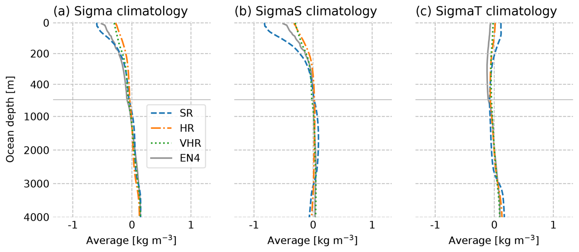
Figure A2 March vertical profiles for SR, HR, VHR, and EN4 1948–2023 in the Labrador Sea box for the relative density sigma0 (a), salinity contribution to the relative density sigma0 (b), and temperature contribution to the relative density sigma0 (c) climatologies. These variables have been computed following Eqs. (A1)–(A3).

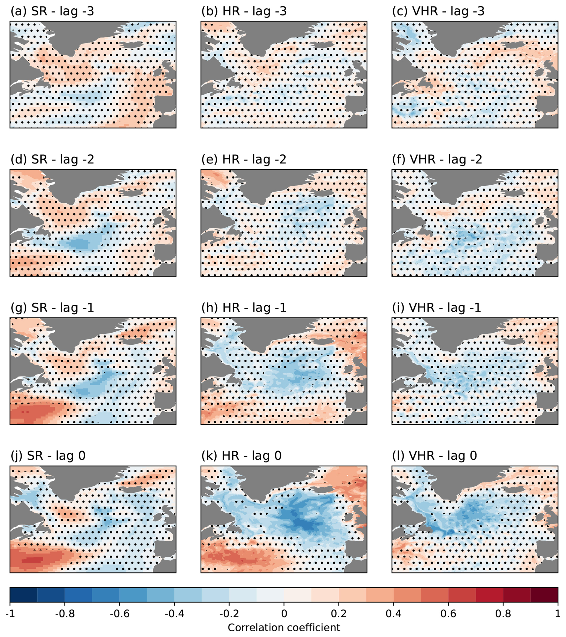
Figure A3 Correlation of March MLD time series with yearly surface temperature for SR (a, d, g, j), HR (b, e, h, k), and VHR (c, f, i, l); lagged 3 years (a–c), lagged 2 years (d–f), lagged 1 year (g–i), and no lag (j–l). Non-significant values are masked with dots to improve the visibility over the significant areas.

Figure A4 Standard deviation of the volume overturning streamfunction without the Ekman transport in sigma2 space for SR (a), HR (b), and VHR (c).

Figure A5 Depth of the maximum correlation between 400 and 1400 m of yearly density with MLD. Complementary to Fig. 8. The black line (a–c) shows the position of the depth vs. longitude sections computed in Fig. A6.

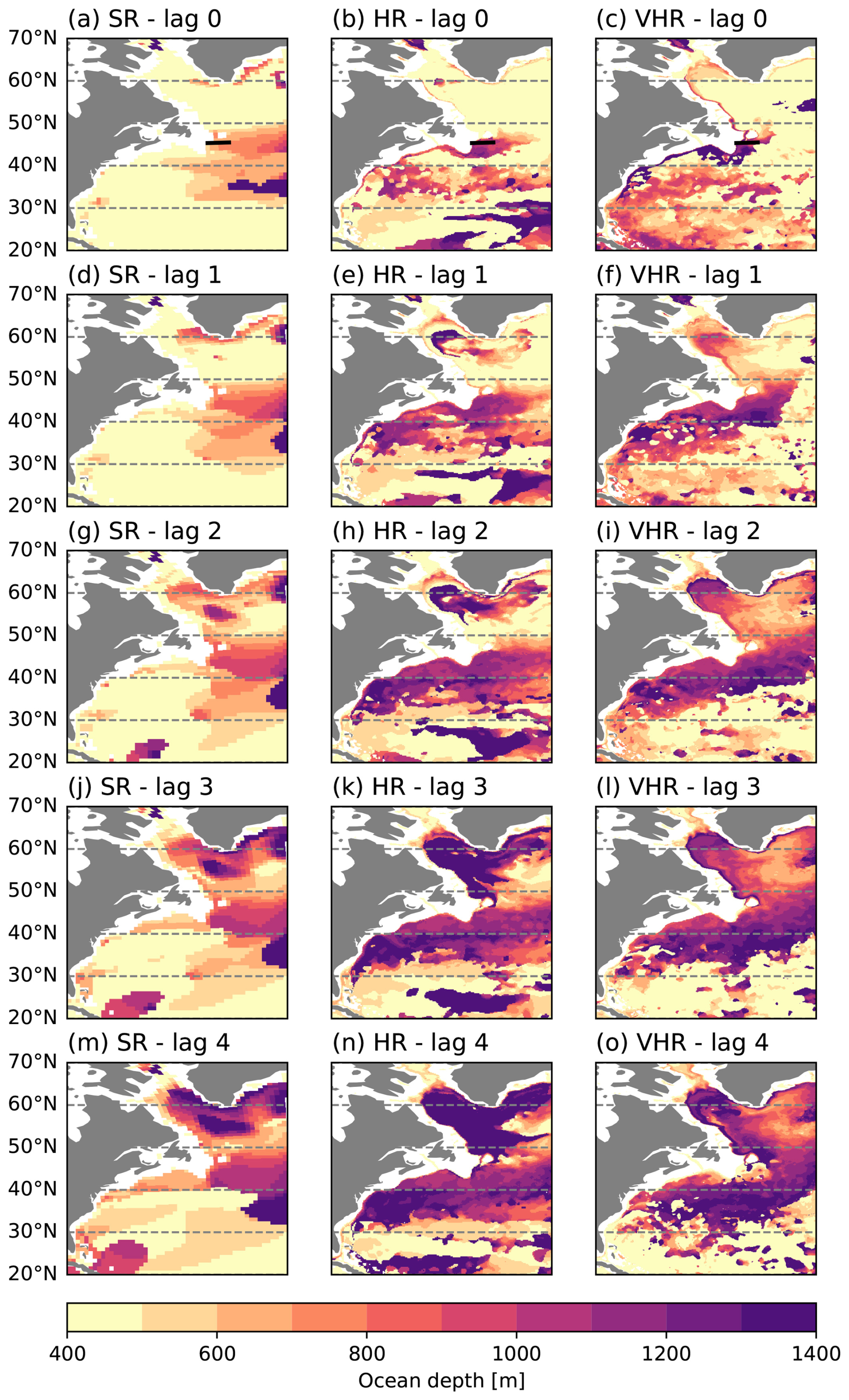
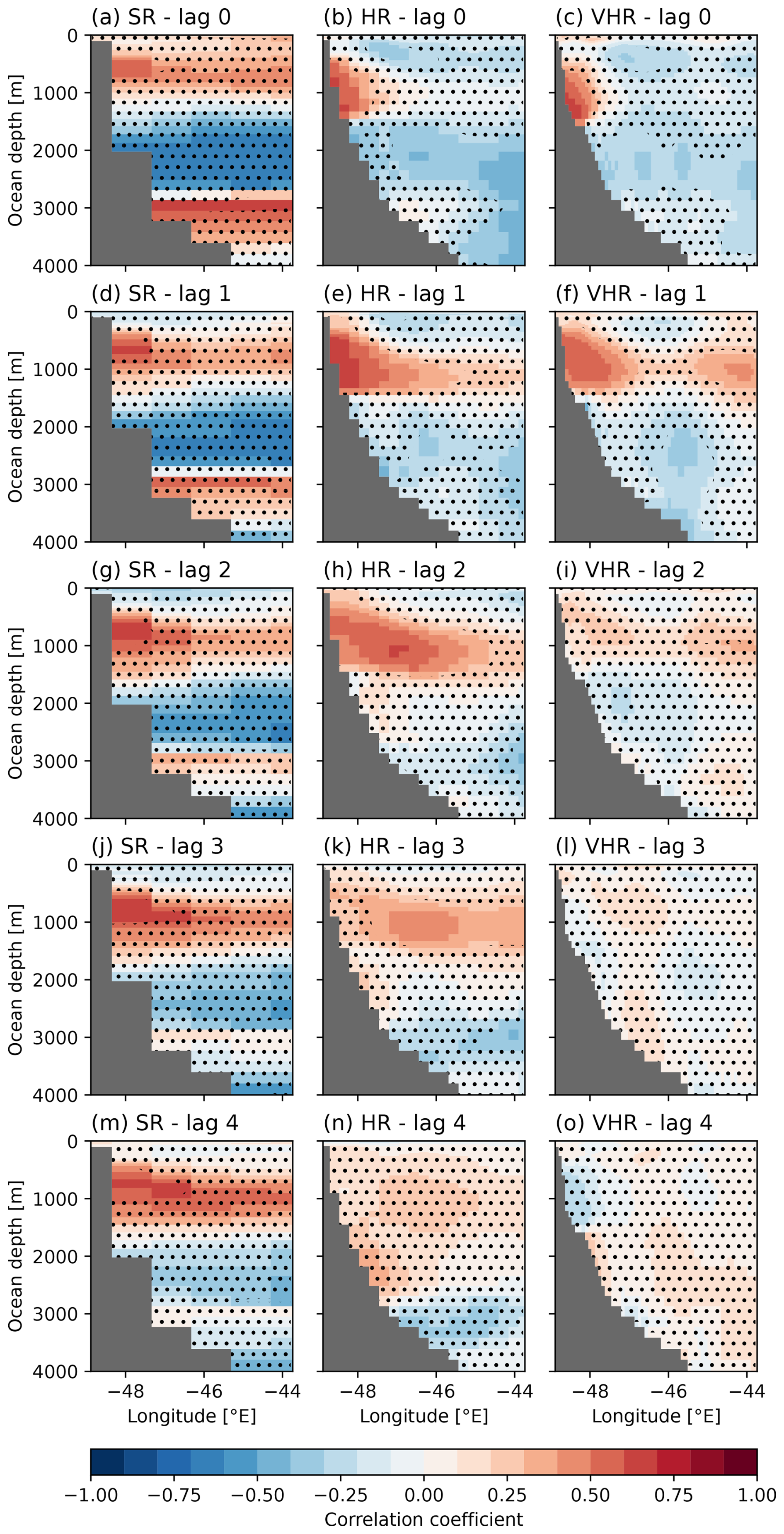
Figure A6 Correlation of March MLD time series with yearly sigma2 at 45.3° N for SR (a, d, g, j), HR (b, e, h, k), and VHR (c, f, i, l); no lag (a–c), 1-year lag (d–f), 2-year lag (g–i), 3-year lag (j–l), and 4-year lag (m–o). Non-significant values are masked with dots to improve the visibility over the significant areas. The section is shown with a black line in Fig. A5a–c.