A causality-based method for multi-model comparison: application to relationships between atmospheric, oceanic and marine biogeochemical variables

We introduce a novel causality-based approach to compare Earth system model outputs. The method is based on the PCMCI+ algorithm, which identifies causal relationships between multiple variables. We aim to investigate the causal relationships between atmospheric (North Atlantic Oscillation – NAO), oceanic (gyre strength, stratification, circulation) and biogeochemical variables (nitrate, iron, silicate, phosphate and net primary production) in the North Atlantic subpolar gyre. It is a critical region for the global climate system with a well-characterised multi-year variability in physical and biogeochemical properties in response to the North Atlantic Oscillation. We test a specific multivariate conceptual scheme, involving causal links between these variables. Applying the PCMCI+ method allows us to differentiate between the influence of vertical mixing and horizontal advection on nutrient concentrations and spring bloom intensity, as well as to highlight model-specific dynamics. The analysis of the causal links suggests a dominant contribution of winter vertical mixing to nutrient concentration compared to transport. The strength of the links is variable among models. Stratification is identified as an important factor controlling spring bloom net primary production (NPP) in some, but not all, models. Horizontal transport also significantly influences nutrient concentration. However, horizontal transport generally exhibits lower contributions than vertical mixing to nutrient variability. The limitations of the method are discussed, and directions for future research are suggested.

1 Introduction

Earth system models (ESMs) are essential tools in climate science. They are designed to unravel the intricate workings of the planet's climate system. The simulation of historical and present dynamics has proven to be skilful in many aspects, including the representation of ocean physics and marine biogeochemistry (Flato et al., 2013; Séférian et al., 2020; Vautard et al., 2021; Tsujino et al., 2020). Despite advances in complexity, ESMs simplify the real world, and this is a source of errors and uncertainties. These models create their own climate system shaped by specific spatial resolutions and parameterisations of various physical, chemical or biogeochemical processes. Multiple reasons explain the differences in architecture between models (Bonan and Doney, 2018): the constraint of computational efficiency which calls for the parameterisation of small-scale processes unresolved by the large-scale variables in the model but also the selection of which processes to include. Given the inherent complexity of the climate system encompassing a myriad of processes currently impossible to be represented in a model, these disparities can lead to differences in future climate states and dynamics with scattered projections (e.g. Kwiatkowski et al., 2020; Tebaldi and Knutti, 2007; Flato et al., 2013; Zelinka et al., 2020).

Intercomparing model output is essential to characterise inter-model differences and to identify the uncertainty around projected values.

Most model intercomparison studies still rely on the analysis of the spatial and temporal distribution of selected model outputs presented as maps of mean values and their range, along with the computation of statistics (e.g. extremes, variability) (e.g. Wang et al., 2020; Flato, 2011; Jacob et al., 2007; Chen and Knutson, 2008). For intercomparisons targeting the historical period, observations or reanalyses are commonly used as references. Model performance is evaluated against real-world data or derived products, and bias maps are used to locate model differences (e.g. Séférian et al., 2020; Yool et al., 2021; Chen and Knutson, 2008; Schaller et al., 2011). However, none of these methods characterises the interactions between variables or quantifies their differences between models. Two recent approaches try to address these limitations. First, the emergent constraint framework is increasingly applied to biogeochemical variables to reduce projection spread (Goris et al., 2023; Kwiatkowski et al., 2017; Fu et al., 2016). This approach identifies relationships between observable present-day variables and specific behaviours in future projections across models, helping to constrain uncertainties in climate predictions. Second, correlation-based approaches have been developed to intercompare models and analyse the interactions between variables (e.g. Charakopoulos et al., 2018; Anagnostopoulos et al., 2010; Gleckler et al., 2008). However, while both these methods provide valuable insights, they fail to identify causal links between variables.

To overcome the limitations of correlation-based methods, Krich et al. (2020) and Nowack et al. (2020) employed a causality approach to analyse or evaluate model output. Here, we extend these earlier studies to the analysis and comparison of multi-model output. The causality framework allows us to describe model differences in a novel way, potentially revealing model-specific dynamics and quantifying the strength of interactions and its range across Earth system models.

Our study focuses on the subpolar North Atlantic, a critical region for the global climate system with a well-characterised multi-year variability in physical and biogeochemical properties in response to the North Atlantic Oscillation, the dominant mode of regional climate variability (Yamamoto et al., 2020; Feucher et al., 2022; Keller et al., 2012; Tjiputra et al., 2012). At the seasonal timescale, deep winter mixing replenishes the sunlit surface ocean in nutrients and sustains an intense spring bloom. The subpolar North Atlantic is also a region undergoing rapid changes including freshening and cooling (Tesdal et al., 2018; Holliday et al., 2020), with potential impacts on large-scale circulation (Fox-Kemper et al., 2021; Hakkinen and Rhines, 2004). Along with these physical changes, an important variability in surface ocean nutrient levels has been documented (Johnson et al., 2013; Hátún et al., 2017) potentially foreshadowing future changes in primary productivity under climate change.

The impact of climate change on net primary production (NPP) in the North Atlantic region remains highly uncertain with a larger spread between model projections compared to other regions (Tagliabue et al., 2021; Fu et al., 2022). While vertical mixing is crucial for injecting nutrients into the productive surface ocean and fuelling primary production (D'Asaro, 2008; Williams et al., 2006), recent studies highlighted the contribution of horizontal transport to observed and projected variability in nutrients and primary production (Whitt and Jansen, 2020; Kwiatkowski et al., 2020; Hátún et al., 2017). The eastern part of the subpolar North Atlantic was proposed by Hátún et al. (2017) as a key area for the mixing of nutrient-poor subtropical waters into the subpolar North Atlantic gyre. The variability in the gyre circulation would be one mechanism controlling the advection and mixing of nutrients and ultimately NPP at regional scale. Moreover, Pelegrí et al. (1996) and Williams et al. (2011) highlight the contribution of subsurface nutrient-rich waters of subtropical origin (the nutrient streams) as a source of nutrients to the subpolar Atlantic through vertical mixing.

This study targets the eastern subpolar North Atlantic and seeks to differentiate between the variability in vertical mixing and horizontal advection of nutrients as controls of fluctuations in NPP. It draws on an ensemble of Earth system model simulations to explore causal links from atmospheric processes to marine biogeochemistry. We rely on the “PCMCI+” method (Runge et al., 2019) for the analysis of causal interactions represented as causal graphs. In these graphs, nodes represent variables and edges indicate potential causal links with associated strengths. Our objective is twofold: (1) to propose a novel approach for model intercomparison and (2) to understand model-specific causal links between variability in atmospheric processes, advection and vertical mixing of nutrients to the surface ocean and NPP.

This article is structured as follows: Sect. 2 describes the causality discovery algorithm we use as well as the conceptual scheme that guides our study. Section 3 details the data used and the pre-processing steps applied to each variable. Section 4 presents the results obtained, highlighting specific key links and their similarities and differences between models. Section 5 discusses the limitations of the method employed, providing details on its strengths and weaknesses. Results are discussed in Sect. 6, and Sect. 7 concludes this article as well as proposes future perspectives.

2 Methodology

2.1 Causality approach: PCMCI+

To investigate the causal links between the variables in our study, we use the PCMCI+ method (Runge et al., 2019; Runge, 2020). This approach is based on Granger causality (Granger, 1969), which examines whether past values of variable A enhance the prediction of B beyond what B's previous values can predict by themselves. PCMCI+ generates a causal graph where physical and biogeochemical variables form the nodes, while edges represent contemporaneous or lagged relationships between these variables (a conceptual example of a causal graph is given in Fig. S1). Each causal link is characterised by a time lag (0 for contemporaneous relationships) and a strength ranging from −1 to 1, with the sign indicating whether the relationship is positive or negative and the value indicating the intensity of the relationship. To detect these causal relationships, the method relies on the concept of conditional independence. Two variables A and B are conditionally independent given a variable C if knowledge of B provides no additional information about A when C is already known. In other words

$$\begin{array}{}\text{(1)}& A⟂⟂B|C⟺P(A|B,C)=P\left(A\right|C).\end{array}$$

In our analysis, this concept is applied through partial correlation tests which evaluate whether the relationship between two variables persists when the influence of one or more conditioning variables is removed. The partial correlation is computed by first performing regressions of both variables on the conditioning set and then calculating the correlation between their residuals. The algorithm proceeds in two main steps: PC (“Peter and Clark”) and MCI (“momentary conditional independence”). The PC step first identifies potential relationships between variables through a series of conditional independence tests. The most significant relationships are then validated during the MCI step, which examines indirect influences between variables. For example, let us assume that NAO (North Atlantic Oscillation) is identified as a parent (explanatory variable) of mixed-layer depth (MLD) and that transport and MLD are parents of nutrients. Then, when testing the link between nutrient and transport, we will not condition by MLD but by NAO, the parent of MLD. For a detailed description of the PCMCI+ method, we refer to Runge (2020). The variables of the conceptual scheme discussed in Sect. 2.3 will be given to PCMCI+, and the resulting causal graphs for different climate models will be compared to each other.

It is important to note that the absence of a statistically significant causal link in our analysis should not be interpreted as definitive evidence for the absence of any relationship between variables. Rather, it indicates that any potential relationship is not strong enough to be significant through this analysis.

2.2 Quantification of causal graph: dissimilarity measure

The output of PCMCI+ is a causal graph with a set of nodes (the variables given to PCMCI+) and potential edges (i.e. causal relationships) between those nodes. We can look at the PCMCI+ results via the adjacency matrix M representing the presence and strength of links between nodes. To compare the graphs (i.e. the relationships within models), it is then possible to compute dissimilarity metrics between adjacency matrices. However, many of these measures have limitations that make them inappropriate in our case. Firstly, the methods often assume an edge's weight to be positive (e.g. Wicker et al., 2013; Koutra et al., 2013), which is not suitable in our case, as our edges can be positive or negative.

The second problem is that the lag associated with the link also has to be taken into account. Even if different, when the lags are close, the distance should be small. On the other hand, once we exceed a certain difference in terms of lags, we can consider the link to be already so different that an even bigger difference in terms of lags will not give a bigger distance. To address these limitations, we propose an alternative approach that allows for negative weights and lags.

An Euclidean distance (as dissimilarity) allows us to deal with the weights of positive and negative edges denoted w_ij, where $i,j\in \textcolor{red}{}\mathrm{0},N\textcolor{red}{}$. To account for the lags, we extend the matrices M from size N×N to size $N\times N\times T$ by adding a third dimension, indicating the lag at which the link occurs:

$$M[i,j,t]=\left\{\begin{array}{ll}{w}_{ij},& \text{if there is a link from }i\text{ to }j\text{ with a lag }t\\ \mathrm{0},& \text{otherwise.}\end{array}\right.$$

Next, each vector M[i,j] is blurred with a Gaussian filter convolution. The kernel K is a Gaussian blur 3×1 ($\left[\frac{\mathrm{1}}{\mathrm{4}},\frac{\mathrm{1}}{\mathrm{2}},\frac{\mathrm{1}}{\mathrm{4}}\right]$). For the convolution operation, we use full padding, which extends the input vector by a total of two elements (size of kernel minus one), adding one element at each end. We note M^′ the matrix after the application of the Gaussian filter convolution. This approach helps us to consider the lag difference by blurring the links in the third dimension, similar to how a blur would make two red squares on blank images share some red pixels if they are close enough. If we consider an example where $M[i,j]=[w_{ij},\mathrm{0},\mathrm{0},\mathrm{0}]$ (i.e. a relationship from i to j only at t=0), the transformed vector $M^{\prime }[i,j]$ is thus given by

$$\begin{array}{rl}{M}^{\prime }[i,j]& =M[i,j]\cdot \left[{\displaystyle \frac{\mathrm{1}}{\mathrm{4}}},{\displaystyle \frac{\mathrm{1}}{\mathrm{2}}},{\displaystyle \frac{\mathrm{1}}{\mathrm{4}}}\right]=[w_{ij},\mathrm{0},\mathrm{0},\mathrm{0}]\cdot \left[{\displaystyle \frac{\mathrm{1}}{\mathrm{4}}},{\displaystyle \frac{\mathrm{1}}{\mathrm{2}}},{\displaystyle \frac{\mathrm{1}}{\mathrm{4}}}\right]\\ & =\left[{\displaystyle \frac{w_{ij}}{\mathrm{4}}},{\displaystyle \frac{w_{ij}}{\mathrm{2}}},{\displaystyle \frac{w_{ij}}{\mathrm{4}}},\mathrm{0},\mathrm{0},\mathrm{0}\right].\end{array}$$

The Euclidean distance can then be applied to the blurred vectors/matrices, considering both the variations in lags and strengths. Our new dissimilarity measure DIS between two (blurred) adjacency matrices M₁ and M₂ can thus be written as

$$\begin{array}{}\text{(2)}& \text{DIS}({\mathbf{M}}_{\mathrm{1}},{\mathbf{M}}_{\mathrm{2}})=\sqrt{\sum _{(i,j,k)}\left({\mathbf{M}}_{\mathrm{1}}^{\prime }\right[i,j,k]-{\mathbf{M}}_{\mathrm{2}}^{\prime }[i,j,k]{)}^{\mathrm{2}}}.\end{array}$$

With this dissimilarity, we take into account how different the lags are for the same link while also taking into account the difference in intensity (strength of interaction). As an example, consider three causal graphs that are identical except for a single causal link with different time lags: k₁, k₂ and k₃, where $k_{\mathrm{1}}<k_{\mathrm{2}}<k_{\mathrm{3}}$. The convolution ensures that the dissimilarity measure reflects the temporal proximity of these lags, such that $\text{Dis}({\mathbf{M}}_{\mathrm{1}},{\mathbf{M}}_{\mathrm{2}})<\text{Dis}({\mathbf{M}}_{\mathrm{1}},{\mathbf{M}}_{\mathrm{3}})$. However, when an expert considers that two time lags k₁ and k₂ are sufficiently distant from each other, they can adjust the convolution kernel size (set to three in our study) to reflect this assessment. Specifically, by choosing a kernel size smaller than the difference between k₂ and k₁, the dissimilarity between models M₁ and M₂ becomes maximal. In this case, the expert effectively indicates that the temporal distance between these lags is so significant that both M₂ and M₃ should be considered equally dissimilar from M₁, resulting in $\text{Dis}({\mathbf{M}}_{\mathrm{1}},{\mathbf{M}}_{\mathrm{2}})=\text{Dis}({\mathbf{M}}_{\mathrm{1}},{\mathbf{M}}_{\mathrm{3}})$. Here we selected a width of 3 years because we consider that lag differences beyond 3 years reach maximum dissimilarity. The width of the kernel is a user-defined parameter that can be changed for specific studies.

2.3 Conceptual scheme

We selected the eastern subpolar North Atlantic (Fig. 1) as a test case for this study focusing on the comparison of physical–chemical drivers of spring bloom dynamics in an ensemble of ESMs through a causality approach. The region is known for its large variability in contemporary nutrient concentrations (Johnson et al., 2013; Hátún et al., 2017). The latter has been linked to the strength of the subpolar gyre circulation through its control on the inflow of nutrient-poor subtropical waters (Hátún et al., 2017). Fluctuations in gyre circulation in turn are driven by regional atmospheric forcing, leading to a causal chain from atmospheric processes to ocean dynamics and finally biogeochemistry.

This region is also prone to a great sensitivity to climate change with a high spread of projected values of primary production. However, the mechanisms behind the projected impacts of climate change on NPP are not well understood (Kwiatkowski et al., 2019; Tagliabue et al., 2021). While vertical mixing is crucial for injecting nutrients to the productive surface layers and fuelling NPP (e.g. deepening of the mixed layer during winter for nutrient supply and spring stratification for the initiation of the bloom), changes in subsurface nutrients brought by horizontal transport are also important and are likely to contribute to the between-model spread of projected NPP (Whitt and Jansen, 2020; Kwiatkowski et al., 2020; Johnson et al., 2013). Our conceptual scheme aims to highlight model-specific representations of the chain of causality running from atmospheric forcing to NPP. It attempts to disentangle the respective contributions of variability in vertical mixing and horizontal transport to modelled fluctuations in nutrient levels and NPP in the eastern North Atlantic basin (Fig. 1).

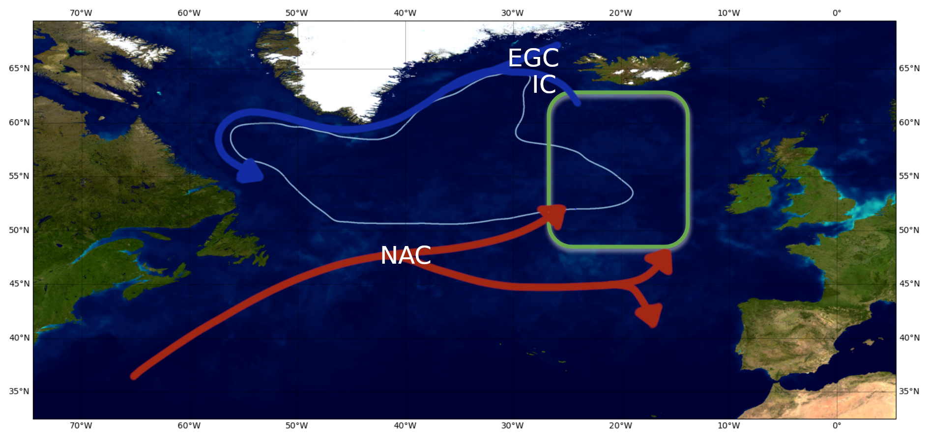
Figure 1 Study area “eastern North Atlantic subpolar gyre” (green square). The main surface circulation patterns are indicated by the arrows (inspired by Daniault et al., 2016). IC stands for Irminger Current, EGC for East Greenland Current and NAC for North Atlantic Current. The gyre corresponds to the zone in light blue. Map credit: NASA-Visible Earth – The Blue Marble: Land Surface, Ocean Color and Sea Ice.

The anticipated chain of causality is represented as a conceptual scheme in Fig. 2. The target variable is the NPP of the spring bloom. Predictors of its variability include atmospheric and ocean physical processes but also nutrient concentrations (nitrate, silicate and dissolved iron). Atmospheric processes are represented by the North Atlantic Oscillation (NAO), a prominent mode of regional climate variability and an important driver of variability in ocean physical and biogeochemical dynamics (Yamamoto et al., 2020; Feucher et al., 2022; Keller et al., 2012; Oschlies, 2001; Herceg-Bulić and Kucharski, 2014; Delworth and Zeng, 2016). Physical processes included are vertical and horizontal transports. Wintertime deepening of the mixed layer injects nutrients to the surface ocean, replenishing the pre-bloom surface nutrient stock (Williams et al., 2006). Stratification during spring and the shoaling of the mixed layer contribute to initiate the spring bloom. Mixed-layer depth (MLD) and stratification are thus chosen as predictors of vertical transport. For the advection of nutrients we will focus on the net transport into the area of study, as well as consider the strength of the North Atlantic subpolar gyre. Lastly, four nutrients are considered: nitrate, phosphate, silicate and dissolved iron.

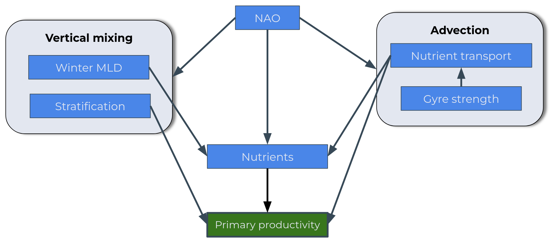
Figure 2 Suggested conceptual scheme. The target variable is in green, and the explanatory variables are in blue.

We anticipate numerous interconnections across the scheme. The NAO is known to exert influence over multiple processes in the North Atlantic, affecting physical variables such as gyre strength, water transport and MLD (Yamamoto et al., 2020; Feucher et al., 2022) but also nutrient concentrations. Diving into the oceanic variables, the gyre strength, relevant for physical variables such as MLD (Swingedouw et al., 2021), could as well be explanatory for nutrient concentrations (Hátún et al., 2017; Johnson et al., 2013) through its impact on nutrient transport. For the vertical mixing component of the scheme, a link from MLD to nutrient concentrations is anticipated because winter MLD deepening is crucial for replenishing the nutrient stock (Williams et al., 2006). We also expect a relationship between stratification and NPP because high stratification during the productive period will inhibit the upward mixing of nutrients and thus NPP (Lozier et al., 2011; Tagliabue et al., 2021). The scheme will be explored for each nutrient (nitrate, dissolved iron and silicate), and we anticipate differences in the intensity of the relationships for each nutrient, especially for the relationship between nutrient and productivity.

3 Experimental set-up

3.1 Selection of Earth system models and simulations

We selected a set of Earth system models with biogeochemical models of similar complexity to explore the variability in causal links connecting atmospheric processes to NPP. These biogeochemical models include at least two phytoplankton functional types (PFTs) with model-specific parameterisations of interactions between PFTs, as well as nutrient limitation of phytoplankton growth. We made sure not to repeat the coupling of ocean and biogeochemical models twice. This led to the selection of the six Earth system models presented in Table 1. There is nevertheless some redundancy in our selection with four ESMs sharing the same ocean model (three with the same version). Additional information on the biogeochemical models is available in the Supplement.

Boucher et al. (2020)Danabasoglu et al. (2020)Lovato et al. (2022)Swart et al. (2019)Christian et al. (2022)Sellar et al. (2019)Yool et al. (2021)Hajima et al. (2020)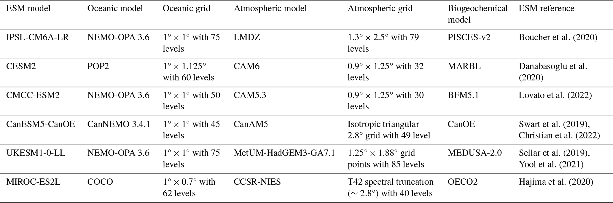

Table 1 Models used in the study.

We selected pre-industrial control simulations (piControl) from the Coupled Model Intercomparison Project Phase 6 (CMIP6) (Eyring et al., 2016). These simulations were run for 500 years with constant natural external forcings (e.g. volcanoes, solar radiation, greenhouse gases) fixed at pre-industrial levels. It allows access to an extended period for assessing model specificities through causal graphs. Due to the absence of variability and trend in external forcings, climate variability is restricted to its unforced internal component. The primary mechanisms driving interactions between spring productivity and its controlling factors are expected to maintain consistent relationships over the 500-year simulation period, though their relative strength may show some temporal variations.

3.2 Definition and pre-processing of variables for PCMCI+

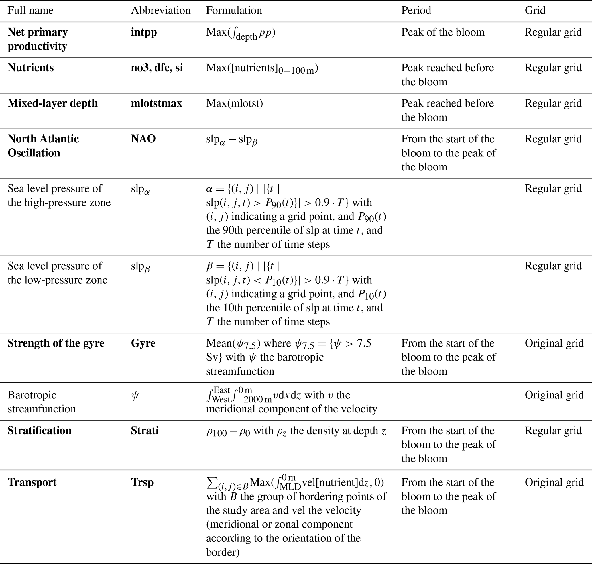
We compute time series of annual means from monthly output fields for each model variable. From these time series variables for PCMCI+ are computed as described below. Each processed variable is centred (mean at 0) and reduced (standard deviation at 1) prior to running PCMCI+. Variables selected for PCMCI+ and their definition are presented in Table 2. The following paragraphs add details to the pre-processing. With the exception of the transport of nutrients and the subpolar gyre index which are computed on the original model grid, all other variables are interpolated on a regular 1° × 1° grid prior to pre-processing.

Table 2 Variables and their formulation. The variables used in PCMCI+ are in bold.

3.2.1 Bloom and productivity

We focus on the variability in the maximum of NPP reached during the year. This corresponds to the maximum reached during the spring months, the spring bloom. For several other variables (e.g. atmospheric forcing, nutrient transport, gyre circulation) it is important to time the start of the bloom as their variability during the bloom might impact bloom dynamics. Following the threshold method in Brody et al. (2013) we consider the bloom to have started once a certain threshold has been exceeded. This threshold value corresponds to the median NPP plus 5 %. The starting date for the bloom is the first month m verifying Eq. (3):

$$\begin{array}{}\text{(3)}& \text{intpp}\left(m\right)>\mathrm{1.05}\times \text{median(intpp)}.\end{array}$$

3.2.2 Nutrients

The study focuses on nitrate, phosphate, silicate and dissolved iron before the beginning of the bloom to qualify the biogeochemical context of the spring bloom. Specifically, we will consider the average concentration in the upper 100 m of the water column. When the bloom starts, nutrient concentrations of the pre-bloom period begin to decline. The timing of the spring bloom varies across different regions and models, as does the timing of the maximum nutrient concentration. Therefore, we will define our annual signal as the peak (i.e. maximum) concentration reached during the winter–spring season. This approach will allow us to capture the yearly variability in nutrient concentrations associated with the intensity of the spring bloom.

3.2.3 North Atlantic Oscillation

The NAO (North Atlantic Oscillation) index quantifies the difference between the high- and low-pressure zones in the North Atlantic region. However, the location of the high- and low-pressure centres varies among different climate models, making it necessary to use a model-independent method for its computation. Historically the NAO was computed as the difference in sea level pressure (slp) between two specific stations (Lisbon, Portugal, and Stykkishólmur, Iceland) (Hurrell et al., 2003). Nowadays, the use of empirical orthogonal function (EOF) over a large geographic area has become common (Hurrell et al., 2003; Hurrell and Deser, 2010). We preferred using the method consisting of computing the difference in slp on two selected zones (Hurrell, 1995; Hurrell et al., 2003), but the selection of the zone needs to be model-independent.

Our proposed solution to select the zones here uses a counting approach. At each time step, the points belonging to the higher and lower 10th percentiles of sea level pressure are identified. For each of these points, the counting index for the high and low pressure is incremented accordingly. As a result, each point is associated with two numbers α and β indicating how many times it belonged to the high- (α) or low-pressure zone (β). To compute the NAO index, we consider the 10th percentile for respectively α and β as the high- and low-pressure areas to compute the sea level pressure difference. In the end, we consider the zones that were most of the time high or low pressure as the high- and low-pressure poles. We display the poles selected for each model in the Supplement (Fig. S3). The selected period for computing the index was from the start to the peak of the bloom. Choosing this period ensures coherence with the other variables considered during this period (e.g. gyre circulation, nutrient transport).

3.2.4 Gyre index

The gyre circulation is characterised by the gyre index, which is computed on the months between the start and the peak of the bloom as it is linked to the NAO (Hurrell and Deser, 2010; Koul et al., 2020). The stream function is computed over 2000 m depth on the original grid and integrated from east to west. Once obtained, a threshold of 7.5 Sv is applied on each grid point as in Biri and Klein (2019). From this method we extract the strength, i.e. the mean of the stream function at the selected point. The shape of each model gyre and its geographical variability are displayed in the Supplement in Fig. S2.

3.2.5 Vertical mixing

The MLD depth in winter will determine the stock of nutrients available (Williams et al., 2006) for the spring bloom. Here we want to capture the variability in MLD intensity. Therefore, we focus on the maximum depth reached between November and April. The impact of stratification on NPP is an important aspect of our study, and we will quantify this relationship using the difference in density as an indicator (Lozier et al., 2011; van De Poll et al., 2013). We focus on the difference in density between 100 m and the surface ρ₁₀₀−ρ₀. To assess the impact of stratification on productivity, we will calculate the mean value of ρ₁₀₀−ρ₀ from the beginning to the peak of the bloom. This approach will allow us to examine the relationship between stratification and NPP during the most active period of phytoplankton growth.

3.2.6 Nutrient transport

The inflow of nutrients via horizontal advection is also an important factor to consider for the nutrient concentration at the start of the bloom and the resulting NPP. We integrate the transport of nutrients from the ocean surface to the mixed layer depth (MLD) for each model. For each depth level and each month considered (between the beginning of the bloom and the peak of the bloom), the nutrient concentration is multiplied by the transport. The transport is computed from the meridional and zonal velocity variable. For our analysis, we will focus only on the inflow of nutrients into our study region. As for the period selected for the signal we will take the transport of nutrients from the beginning of the bloom to the peak of the bloom.

4 Results

We obtain one distinct causal graph for each nutrient: nitrate, dissolved iron and silicate. With the exception of CanESM5-CanOE for which silicate was not available, all three nutrients are considered for the remaining models. Causal links differ slightly between nutrients. For example, for a given link between two variables, the nutrient may not be directly involved but may indirectly influence the relationships through changes in conditioning variables, resulting in slight variations in the calculated strength. Nutrients are identified in the following by adding “_no3” (nitrate), “_dfe” (dissolved iron) or “_si” (silicate).

4.1 Similar models

The similarity between models is evaluated based on the dissimilarity introduced earlier. Looking at the dissimilarity of the entire causal graph could mask important local differences. Focusing on sub-matrices provides insight into differences between models with respect to specific relationships. For instance, when analysing dynamics around a specific variable (the ith one), we can extract its corresponding column (the ith column) from the complete PCMCI+ matrix. This column represents all causal influences from the ith variable on the other variables in the system. By applying our dissimilarity measure to these extracted columns from different models, we can systematically compare how various models represent the causal influences linked to this specific variable. Figure 3 represents the dissimilarity between models for links with dfe. UKESM1-0-LL has the largest dissimilarity with other models. These high values of dissimilarity have two possible explanations (interactions between nutrients and lagged links) which will be discussed in Sect. 4.2.

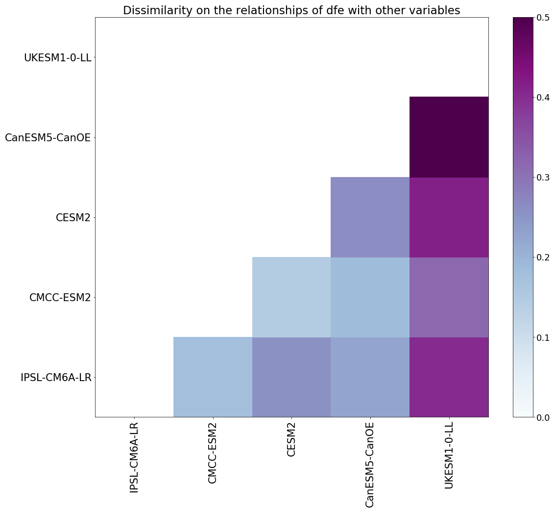
Figure 3 Dissimilarity between each model for iron links only. The darker the colour, the more different the models.

To further quantify the similarity or dissimilarity between models and to identify the corresponding variables, we count how many times two models are the closest to each other or the most different. The results are synthesised in Fig. 4 for IPSL-CM6A-LR with the most and least similar links displayed in Fig. 4. The results for the other models are given in the Supplement from Figs. S4 to S8. From Fig. 4, it appears that CMCC-ESM2 is the closest model, particularly for impacts from NAO, gyre and transport. It has to be noted that the converse is not necessarily true. To understand this, let us consider the most different model on the right of Fig. 4. CESM2 is the most different model from IPSL-CM6A-LR with differences located mainly on gyre and transport, but UKESM1-0-LL also appears to be rather different from IPSL-CM6A-LR. UKESM1-0-LL is also the most different model from all the other models (Figs. S3–S6). However, UKESM1-0-LL obviously also has a model that is most similar, which is CMCC-ESM2, but this similarity is not reciprocal, as UKESM1-0-LL seems to have the most distinct behaviour. CanESM5-CanOE frequently appears as the most different model from UKESM1-0-LL concerning nutrients, gyre, NAO and stratification. Therefore, these two models are the most dissimilar. Grouping models according to their similarity or dissimilarity raises the question of which specific links differ between the models and which links the models agree with. To answer this question, specific contemporaneous links are analysed next (at lag 0).

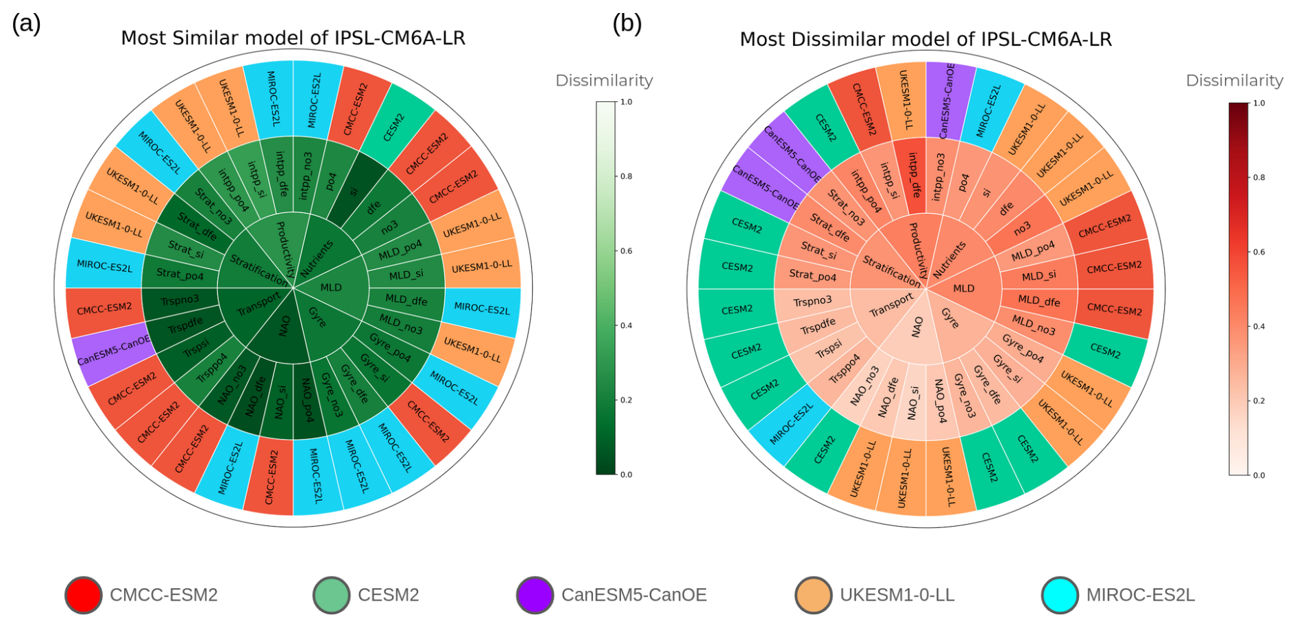
Figure 4 Most similar (a) and dissimilar (b) models compared to IPSL-CM6A-LR based on the dissimilarity metric in Eq. (2). The inner circle indicates the variable, the middle circle shows each variable's variant depending on which nutrient is considered(“_no3” for nitrate, “_dfe” for dissolved iron, “_si” for silicate and “_po4” for phosphate). The outer circle indicates the most similar or dissimilar model. The colour scale in the inner and middle circles represents the dissimilarity intensity, while the outer circle's colour identifies the most similar or dissimilar model.

4.2 Control of nutrients

In the following subsections, we focus exclusively on contemporaneous lags (lag-0 relationships). While lagged relationships were also identified in our analysis, they were less abundant and much weaker and therefore not robust enough to be considered.

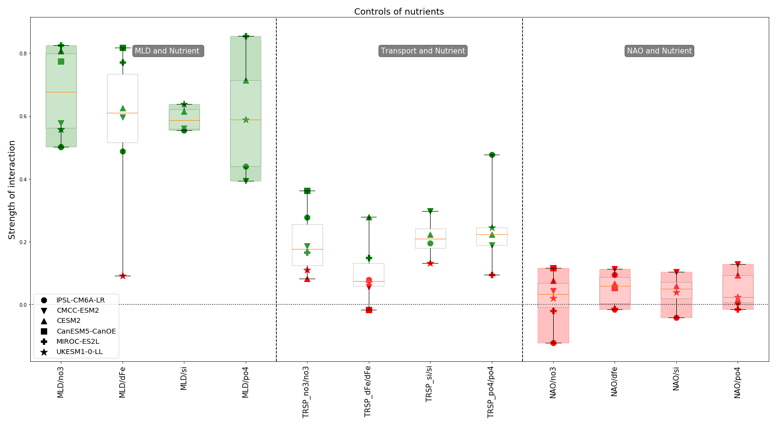
Figure 5 Controls of pre-bloom nutrient concentrations: strength of links for each model with median and quartile values (boxplot). Each marker represents a different model, with the marker colour indicating the statistical significance of the causal link as determined by PCMCI+ (green for significant links, p<α; red for non-significant links, p>α). We define model agreement in two ways: when all models consistently identify a link as significant (boxplot highlighted in green) or when all models consistently identify a link as non-significant (boxplot highlighted in red).

In Fig. 5, we have selected a subset of links that directly control pre-bloom nutrient concentrations. The first panel shows the model agreement for the control of MLD on nitrate and silicate (highlighted in green). As expected, the maximum winter MLD has a strong impact on pre-bloom nutrient concentrations with a consensus between models (mean strength of link: 0.60 for silicate, 0.67 for nitrate and 0.60 for phosphate). This agreement brings coherence among models, although links for nitrate and phosphate (standard deviation of respectively 0.13 and 0.17) are more scattered compared to silicate (standard deviation of 0.04). Regarding iron concentration, UKESM1-0-LL stands out with a non-significant link from MLD to iron concentration. For the other models the strength of the link is of the same order of magnitude as for nitrate and phosphate. This reflects the variability in underlying parameterisations of iron biogeochemistry across Earth system models (Tagliabue et al., 2016). The median strength is about the same for the four nutrients.

The models also agree on the lack of direct impact of NAO on nutrient concentrations. However, it is possible that the NAO indirectly affects nutrient concentrations by impacting a physical variable which in turn influences nutrient concentrations. As discussed in Patara et al. (2011), this intermediary variable could be the advection of nutrients, which is considered here via the transport of nutrients. The intermediary variable could also be the MLD, partially driven by the NAO (Yamamoto et al., 2020), also considered in our scheme. These indirect links will be discussed in Sect. 4.4. Lastly, the influence of nutrient transport on pre-bloom nutrient concentrations is scattered. Models CMCC-ESM2 and IPSL-CM6A-LR agree on a positive impact for nitrate, silicate and phosphate (respectively for CMCC-ESM2: 0.19, 0.3 and 0.19; for IPSL-CM6A-LR: 0.28, 0.19 and 0.47), but neither shows a significant impact on iron. CESM2 also shows a positive impact on silicate (0.23) and phosphate (0.22) and is the only one to have a moderate impact on iron (0.28). The only other model having an impact on iron is MIROC-ES2L with a low intensity (0.15). Concerning this model, nitrate is also affected by transport but also with a low intensity (0.16). CanESM5-CanOE shares some of the behaviour of CMCC-ESM2 and IPSL-CM6A-LR, with a positive impact for nitrate (0.36) and no impact for iron. UKESM1-0-LL is the only one to have no influence from advection except for phosphate (0.24). In CESM2, nitrate is not influenced by advection but is strongly influenced by MLD. In contrast, for other nutrients, MLD has a less strong influence, and a positive impact from transport is observed. This suggests that for nitrate, the strong influence of MLD leaves no opportunity for advection to affect nutrient variability.

A general conclusion of those results is the major importance of vertical mixing for nutrients. While there is a consensus on the importance of MLD for nitrate, silicate and phosphate concentrations, inter-model differences still exist, particularly for iron cycling and nutrient transport.

Figure 6 Same as Fig. 5 but for controls of net primary productivity.

4.3 Productivity drivers

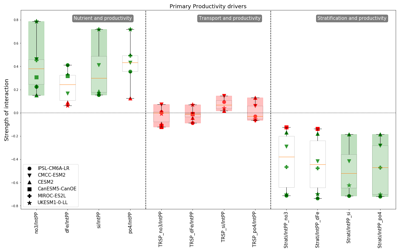
In Fig. 6 we isolated a subset of links between variables known to control NPP and the peak intensity of the spring bloom. The left panel reveals two consistent links among the models: nitrate and NPP, and silicate and NPP. However, while the models agree on the significance of these interactions, they disagree on their strength, with a wide range of values (nitrate: mean of 0.4 and standard deviation of 0.21; silicate: mean of 0.37 and standard deviation of 0.23). We also observe that for phosphate and NPP models are also close to a consensus with a mean at 0.42 and a standard deviation of 0.19. The UKESM1-0-LL model exhibits the strongest links for three nutrients (nitrate: 0.79; silicate: 0.72; phosphate: 0.72), while the CESM2 and IPSL-CM6A-LR models show the weakest, with all values around 0.16 for the same three nutrients. The variability in nitrate, silicate and phosphate concentrations before the bloom has a variable impact on NPP across the selected models. For iron the range of interaction strengths is narrower, with both the CESM2 and UKESM1-0-LL models showing non-significant results. The maximum strength value is 0.41, observed for the IPSL-CM6A-LR model. Notably, the impact of iron variability on NPP in the IPSL-CM6A-LR model is twice as strong as that of silicate or nitrate. Conversely, the CMCC-ESM2 and UKESM1-0-LL models show the opposite trend. For the other models, the strength of this link is lower for iron. The strength slightly decreases for MIROC-ES2L going from approximately 0.46 for nitrate and phosphate to 0.35 for iron. For CMCC-ESM2, the strength decreases from approximately 0.44 for the three other nutrients to 0.17 for iron. The difference is even more pronounced in the UKESM1-0-LL model, which exhibits the strongest links for nitrate and silicate but a non-significant one for iron. In the CESM2 model the strength of those links remains fairly stable, with low strength values for both nitrate and silicate as well as an iron and phosphate residual value (the last partial correlation value obtained which did not pass the significance test) that is close to these.

The last panel of Fig. 6 presents the relationship between stratification during the productive period (from the start to the peak of the bloom) and NPP. With the exception of CanESM5-CanOE, which shows a non-significant link, the impact of stratification is negative across all models, as anticipated. However, the range of interaction strengths is quite broad. The UKESM1-0-LL and IPSL-CM6A-LR models exhibit strong negative links (approximately −0.7), while CESM2 shows a weak strength of around −0.2, and CMCC-ESM2 and MIROC-ES2L have moderate strengths of approximately −0.3 and −0.45. This marked difference in dynamics among the models suggests that they may respond differently to projected climate conditions, as stratification is known to be increasing under global warming (Li et al., 2020). Specifically, if stratification continues to increase and assuming that the relationship will remain unchanged in the future, the intensity of the bloom in the eastern part of the subpolar gyre may decrease more significantly in the UKESM1-0-LL and IPSL-CM6A-LR models.

Lastly, the middle panel of Fig. 6 indicates that nutrient transport does not have a significant direct impact on NPP in any of the models. However, as discussed in the previous subsection, transport plays a role in determining pre-bloom nutrient concentrations for some models (Fig. 5). These nutrient concentrations in turn significantly affect NPP, as shown in the first panel of Fig. 6. Therefore, transport has an indirect impact on NPP via nutrient concentrations. However, this impact is relatively low, as the influence of transport on nutrient concentrations is moderate, and the effect of nutrient concentrations on NPP can also be moderate or strong depending on the model. As a result, two consecutive moderate impacts lead to a rather low overall impact. For instance, if the variability in transport explains 30 % of the variability in nutrient concentrations and the latter explains 30 % of NPP variability, then transport explains 9 % of NPP variability.

Figure 7 Same as Fig. 5 but for selected physical interactions. Other physical interactions are displayed in Fig. S7.

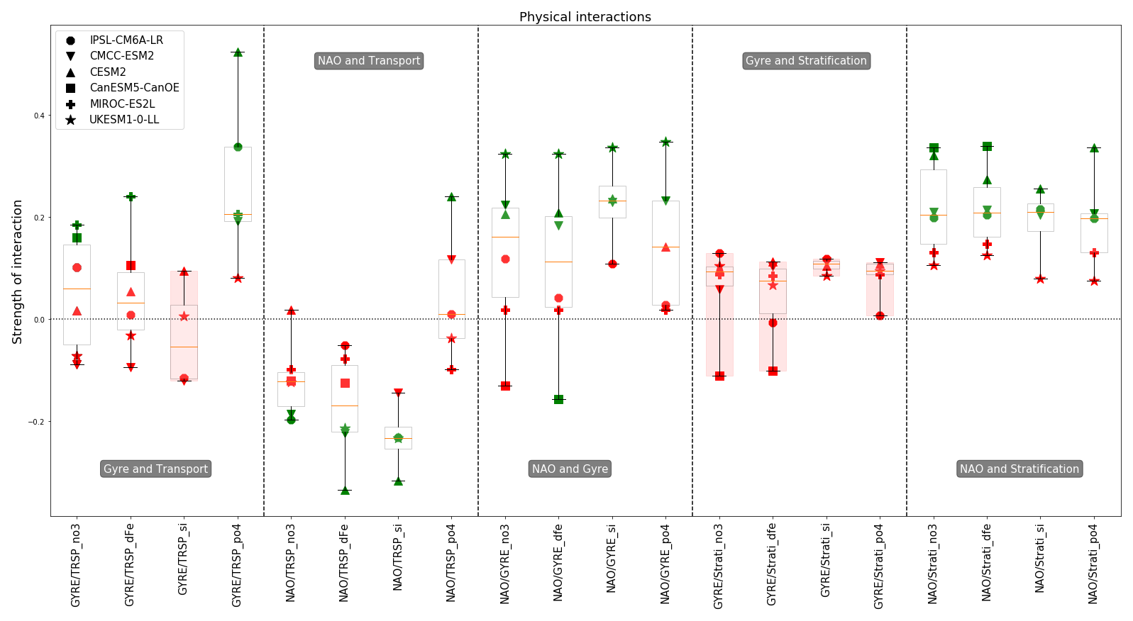
4.4 Physical interactions

Figure 7 presents a subset of physical interactions included in our conceptual scheme. Other interactions are displayed in Fig. S7. The focus of Fig. 7 is on the atmospheric impact on the ocean component, specifically the impact of the North Atlantic Oscillation (NAO) on transport, gyre strength and stratification. For the CMCC-ESM2 model a significant impact of NAO was found for most variables, except for silicate and phosphate transport, which has a residual of around −0.14 and +0.12. The same holds for CESM2, which only misses an impact on nitrate transport with a residual around 0.03. Comparing only these two models, the strength of relationship between NAO and gyre strength is similar (around 0.2), but the impact on transport is slightly stronger for CESM2 (phosphate at approximately +0.24, while silicate and iron at −0.31 for CESM2 and around −0.2 concerning nitrate and iron for CMCC-ESM2). CESM2 also has a stronger effect of NAO on stratification (around 0.3 for CESM2 and around 0.2 for CMCC-ESM2), making it the model with the strongest overall impact from NAO on its oceanic variables.

For the other models many model-specific links were identified, suggesting inter-model differences in dynamics. Starting with UKESM1-0-LL, NAO has a significant impact on the gyre strength (∼0.33) but none on the stratification in our zone. The lack of a significant link between NAO and stratification sets this model apart. It does not result from the approach taken to compute NAO as there are no major differences in the placement of high- and low-pressure zones between UKESM1-0-LL and the other models. The UKESM1-0-LL model also shows significant links from NAO on iron and silicate transport (with a strength of around 0.24, slightly bigger for silicate) but not on nitrate transport (residual around −0.12). The IPSL-CM6A-LR model is the only one with a non-significant impact on gyre strength. However, the NAO significantly impacts stratification (with a strength of about −0.2) and the transport of nitrate and silicate (around −0.22, slightly bigger for silicate).

Lastly the CanESM5-CanOE model, it is the only one with a negative impact of NAO on the gyre as opposed to a positive one observed in the other models (or at least a positive residual when not significant). However, we see in the third panel of Fig. 7 that in the first boxplot it is not significant and in the second one it is. This relationship is on the verge of significance (with a strength of −0.14 when significant). This suggests a potential unique behaviour in this model with respect to the relationship between the NAO and gyre strength. The CanESM5-CanOE model also exhibits one of the strongest impacts on stratification (with a strength of about −0.33). Lastly, the transport of nutrients is not significantly impacted by the NAO.

In the previous results, we identified for all models, except UKESM1-0-LL, the transport of at least one nutrient impacting the variability in nutrient concentrations. Therefore, it is possible for NAO to indirectly influence nutrient concentrations through its impact on transport. This indirect link between NAO and nutrient concentrations is present in IPSL-CM6A-LR, CESM2, CMCC-ESM2 and MIROC-ES2L. In the case of IPSL-CM6A-LR and MIROC-ES2L nitrate and silicate transport significantly impact their respective nutrient concentrations. Likewise, for the CESM2 model, iron and silicate transport significantly affect their corresponding nutrient levels. The CMCC-ESM2 model also exhibits this indirect link through nitrate transport but not for iron transport, as NAO does not impact it. In all these cases the transport variability is partly driven by the NAO. In summary, the indirect link between NAO and nutrient pre-bloom concentration through transport is model-dependent.

Considering the interaction between gyre strength and stratification, we observe that the models agree on the non-significance of these interactions. However, with the notable exception of silicate, the gyre strength impacts nutrient transport. MIROC-ES2L has a significant link of about 0.2 for nitrate, iron and phosphate. The other models only have a link for nitrate or phosphate, and none is found for UKESM1-0-LL. Some models have an indirect influence of gyre strength on nutrient concentration. For example, the interaction between gyre strength and phosphate transport is strong for CESM2 (0.52). In this model, phosphate transport significantly impacts pre-bloom phosphate concentration with a strength of 0.22. Thus, there is an indirect influence of gyre strength on nutrient concentration via nitrate transport. We also observe a marked difference for the dynamics of phosphate transport compared to other nutrients. For three models (IPSL-CM6A-LR, CMCC-ESM2 and CESM2), a significant link is found for phosphate transport without any significant link for other nutrients.

5 PCMCI+ limitations

Like for many other algorithms, it is crucial to carefully select variables given to PCMCI+, as the selection will significantly affect results. It is important to note that PCMCI+ is not intended to be used as a data-mining tool, as stated by Runge et al. (2019). While it is necessary to include all variables containing relevant information, a number that is too high will decrease the performance of the algorithm. To evaluate the decrease in performance as a function of the number of variables and the time lag, two criteria are commonly used: “precision” and “recall”.

• The precision represents the ratio of true positives among all the positives found by the algorithm (true positives + false positives): $\text{precision}=\mathit{\#}\text{true pos.}/(\mathit{\#}\text{true pos.}+\mathit{\#}\text{false pos.})$.

• The recall corresponds to the ratio of true positives among all the positives that the algorithm should have found (true positives + false negatives): $\text{recall}=\mathit{\#}\text{true pos.}/(\mathit{\#}\text{true pos.}+\mathit{\#}\text{false neg.})$.

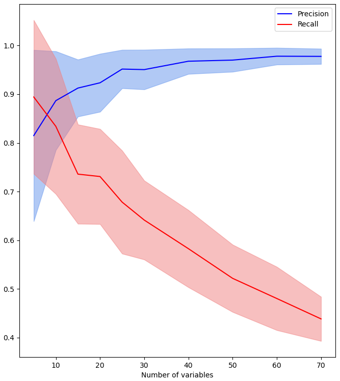
Figure 8 Precision (blue) and recall (red) according to the number of variables with a max time lag fixed at 5.

To quantify the recall and precision performances of PCMCI+, we applied it to artificially generated random auto-regressive vectors. Auto-regressive vectors are time series built so that they depend on past values of themselves. A set of N vectors $(X_i{)}_{\mathrm{1}\le i\le N}$ is defined according to

$$\begin{array}{}\text{(4)}& X_i\left(t\right)=\sum _{\mathrm{0}\le \mathit{\tau }\le {\mathit{\tau }}_{\max }}\sum _{\mathrm{1}\le j\le N}{\mathit{\alpha }}_{i,j,\mathit{\tau }}{X}_j(t-\mathit{\tau }),\end{array}$$

with ${\mathit{\alpha }}_{i,j,\mathit{\tau }}$ being the randomly chosen dependence coefficient and τ_max the maximum lag value. Each non-null random dependence between the variables has been constrained to have a value of at least 0.2. To be close to the configuration of this study, vectors are generated on 500 time steps. The non-null values of α_i,j in these auto-regressive vectors serve as our “ground truth”, allowing us to evaluate the ability of PCMCI+ to correctly identify the presence or absence of causal links.

We tested the performances according to a varying number of variables and 50 times for each number of variables considered. The results are displayed in Fig. 8. The blue curve illustrates that precision is not critical, since an increasing number of variables does not lower it. However, the red curve shows that an increasing number of variables affects the recall. With 60 variables, we retrieve less than half of the expected links (recall criterion). Thus, this experiment clearly illustrates that it is important to give a relatively low number of variables to the algorithm.

Hence, variables need to be selected with great care in order to capture every important feature of the scheme under investigation. In our study, we selected seven variables to consider key elements for our study and to also have a good compromise with the performance by not having too many variables. If certain key variables are omitted from the set of variables given to PCMCI+, there is a risk that some of the causal links found by PCMCI will be incomplete or inaccurate. Forgetting key explanatory variables turns a causality analysis into a correlation analysis.

6 Discussion

PCMCI+ has demonstrated its efficiency in identifying model-specific dynamics and highlighting differences between models that may not be immediately apparent in traditional model output intercomparisons. The PCMCI+ method allowed us to explore multiple conceptual schemes through an iterative process of variable selection. By progressively adding or removing variables it is possible to assess the robustness of relationships between variables. Some relationships remain stable despite changes in the variable set, while others emerge or disappear, establishing the relevance of each variable. We were able to separate the role of vertical mixing and advection on controlling the variability in NPP. Our analysis suggests that vertical mixing plays a more pronounced role in modulating the intensity of spring bloom NPP in the eastern North Atlantic subpolar gyre than horizontal transport, in line with a previous study (Ólafsson, 2003). We also observed that stratification during the bloom serves as a significant inhibitor of bloom intensity (Sarmiento et al., 2004), but this relationship is significantly strong in only two of the five models included in this study (IPSL-CM6A-LR, UKESM1-0-LL). As climate change progresses, it is anticipated that NPP in these models will show a greater sensitivity to increasing stratification (Wilson et al., 2022). Moreover, models that currently show no significant impact of stratification on NPP may exhibit a negative effect appearing as global warming intensifies. This could unveil a novel causal relationship emerging under certain climate change scenarios. This inter-model variability in the response of spring bloom NPP to stratification may contribute to the multi-model spread on projected values of NPP.

Furthermore, the nutrient transport in this study has been computed along the borders of a large region, with each boundary point of the area (Fig. 1) taken into consideration. This transport criterion did not allow us to retrieve a consistent link between the gyre strength and the transport for all the nutrients as discussed in Johnson et al. (2013). In their work, they found an interaction between nitrate and gyre strength and another one, slightly stronger, between phosphate and gyre strength. In our study, we observed more significant relationships for phosphate and fewer for nitrate. However, these criteria allowed us to highlight impacts of NAO on nutrient variability via its impact on transport for most of the models. Addressing this indirect link from NAO to nutrient concentration via the transport underscores the importance of a causality-based approach and the importance of considering key explanatory variables. If we do not consider transport, we may find a spurious link between NAO and nutrient concentration, obscuring a hidden variable. This illustrates results that would have been missed by a correlation-based approach only.

The above highlights the complexity of the North Atlantic subpolar gyre and the potential for indirect relationships between variables. Although the NAO does not directly impact nutrient concentrations, it can still influence nutrient availability through indirect pathways. By examining these indirect links, we obtain a more comprehensive understanding of the dynamics of the North Atlantic subpolar gyre and the factors that control nutrient concentrations and NPP. This also emphasises the additional information gained from a causality-based intercomparison approach compared to a correlation-based intercomparison.

Despite the redundancy of the oceanic component (NEMO) across selected ESMs, with only CESM2 using a different oceanic model (POP2), we do not observe any unique behaviour specific to CESM2 or a commonality shared by the other four ESMs. It is noteworthy that the two models exhibiting the strongest NAO impact, namely CESM2 and CMCC-ESM2, share the same atmospheric model CAM6. Simpson et al. (2020) did not identify a distinct behaviour for this atmospheric model compared to others among CMIP models but did not look at the impact of NAO on specific variables via causality. With our study, it is hard to establish a firm conclusion based on a single member, but applying a causality-based approach to a wider set of simulations using this atmospheric model could offer alternative insights.

The proposed causality-based comparison method also allows inter-model variations in the strength of variable interactions to be quantified. While it is expected that winter mixing influences the pre-bloom nutrient stock, variations between the models still exist. All models agree on the significant role of MLD for silicate within a narrow range of strengths. However, the range is somewhat broader for nitrate and phosphate and even more for iron, with CanESM5-CanOE finding MLD to be not significant. Tagliabue et al. (2016) found a similar result with models having a stronger disagreement for iron. Also, the unique behaviour we observe in the MEDUSA2 model from UKESM1-0-LL is also discussed in this article with an overestimation of surface iron possibly due to a residence time that is too long and a scavenging rate that is too low. We also found a strong auto-correlation for iron (not shown) only for this model which could have the same explanation.

7 Conclusion and perspectives

This study uses a set of Earth system models to explore the interannual variability in nutrients and NPP in the eastern North Atlantic subpolar gyre. This region is characterised by significant mixing and inter-model uncertainty in nutrient and NPP projections. We established a conceptual scheme to determine which mechanism, vertical mixing or advection, is crucial in explaining multi-model dispersion in nutrient and NPP dynamics in this region.

The method allowed us to extract the causal links from a multivariate conceptual scheme. Our findings indicate that vertical mixing during winter is generally more important for peak spring bloom NPP in this region than horizontal transport. However, the influence of vertical mixing on peak spring bloom NPP still has some variability among the models expressed by the spread of the strength of the link. Combined with model-specific dynamics (e.g. NAO impacting transport, transport impacting nutrient concentration), such differences are likely to contribute to inter-model spread. Stratification is identified as an important factor controlling spring bloom NPP in some, but not all, models. As climate change progresses, it is expected that NPP will suffer from increasing stratification with potentially different reactions to it from one model to another.

Despite its limitations, the causality method used in this study has proven effective in identifying model-specific dynamics and highlighting differences between models that may not be immediately apparent based on the usual difference metrics. The proposition of a new dissimilarity measure to be applied on causal graphs has enhanced model comparison by synthesising and quantifying between-model differences.

The method has been verified and can be applied for a variety of purposes such as model evaluation. For example, the comparison of model output and observational data will allow us to identify discrepancies in links and associated strengths, suggesting unrealistic model dynamics. The dissimilarity metric proposed could serve as a validation tool. However, it is essential to acknowledge as the recall of PCMCI+ decreases with increasing variables, an important part of the ground truth (true links existing in the data) can be missed and will add a bias for the validation. While this application is promising, its implementation would require an in-depth investigation of methodological aspects specific to observational data, particularly regarding the handling of false negatives and the phasing of climate events. Another possible application of the PCMCI+ method involves comparing various experiments, such as different climatic scenarios. This approach facilitates the discovery of new dynamics or the observation of changes in the intensity of existing ones, leading to an improved understanding of models' behaviours under different environmental conditions. Applying the method to climate change scenarios will improve our understanding of the inter-model spread of projected variables (e.g. NPP). Future studies could extend this analysis to a larger ensemble of models and simulations, potentially enabling clustering approaches (Couespel et al., 2024) to identify systematic patterns in causal relationships across this larger range of ESMs.