the Creative Commons Attribution 4.0 License.
the Creative Commons Attribution 4.0 License.
 | 11 Jul 2024
Testing the assumptions in emergent constraints: why does the “emergent constraint on equilibrium climate sensitivity from global temperature variability” work for CMIP5 and not CMIP6?
Mark S. Williamson
Peter M. Cox
Chris Huntingford
Femke J. M. M. Nijsse
It has been shown that a theoretically derived relation between annual global mean temperature variability and climate sensitivity held in the CMIP5 climate model ensemble (Cox et al., 2018a, hereafter CHW18). This so-called emergent relationship was then used with observations to constrain the value of equilibrium climate sensitivity (ECS) to about 3 °C. Since this study was published, CMIP6, a newer ensemble of climate models has become available. Schlund et al. (2020) showed that many of the emergent constraints found in CMIP5 were much weaker in the newer ensemble, including that of CHW18. As the constraint in CHW18 was based on a relationship derived from reasonable physical principles, it is of interest to find out why it is weaker in CMIP6. Here, we look in detail at the assumptions made in deriving the emergent relationship in CHW18 and test them for CMIP5 and CMIP6 models. We show one assumption, that of low correlation and variation between ECS and the internal variability parameter, a parameter that captures chaotic internal variability and sub-annual (fast) feedbacks, that while true for CMIP5 is not true for CMIP6. When accounted for, an emergent relationship appears once again in both CMIP ensembles, implying the theoretical basis is still applicable while the original assumption in CHW18 is not. Unfortunately, however, we are unable to provide an emergent constraint in CMIP6 as observational estimates of the internal variability parameter are too uncertain.
- Article
(3859 KB) - Full-text XML
- BibTeX
- EndNote


Since the first general circulation climate models were introduced in the 1960s (Manabe and Bryan, 1969; Manabe and Wetherald, 1975), an ever-increasing amount of effort has been spent developing and improving these models to produce simulations that are increasingly more realistic and feature more of the processes and interactions present in the real world. The progress and understanding of the processes governing the Earth's climate as a result has been impressive. However, even after decades of research, the range of predictions of some key characteristics of the Earth's future climate coming from these models are actually increasing rather than narrowing with time, one particular characteristic being the amount of warming due to doubling of CO2 at equilibrium, known as equilibrium climate sensitivity (ECS, Sherwood et al., 2020). Even though the latest state-of-the-art climate models in the Coupled Model Intercomparison Project 6 (CMIP6, Eyring et al., 2016; CMIP6_database, 2021) have a larger range of ECS values ([1.84; 5.68 K]) than previous CMIP model ensembles (Forster et al., 2020), the latest IPCC estimates have actually narrowed. For decades the IPCC “likely” range for ECS was between 1.5 and 4.5 K. In the latest report (IPCC, 2021) this was reduced to between 2.5 and 4 K with a best estimate of 3 K.
There have been numerous attempts (Knutti et al., 2017) to constrain ECS using the historical warming record, paleoclimate data and climate model experiments. Researchers have also used the emergent constraint technique (Hall et al., 2019; Brient, 2020; Williamson et al., 2021) to constrain ECS (see, for example, Covey et al., 2000; Knutti et al., 2006; Masson and Knutti, 2011a; Hargreaves et al., 2012; Sherwood et al., 2014; Caldwell et al., 2018, and the many references listed in Williamson et al., 2021). The basic idea of emergent constraints is to identify an observable of the climate x that varies significantly across a climate model ensemble and that exhibits a statistically significant relationship f(x) with another variable y describing an aspect of the climate model's future state. The relationship , is referred to as an “emergent relationship” where ε is a relatively small departure from f. Since x is observable, it can be measured in the real world. As such, f may then place a useful constraint on y, provided that the measurement uncertainty in x is small compared to the range of simulated values. This constraint is “emergent” because the emergent relationship f cannot be diagnosed from a single climate model. It becomes apparent only when the full ensemble is analysed.
There are pitfalls with the emergent constraint approach that must be guarded against particularly when the emergent relationships are not founded on well-understood physical processes. For example, data-mining outputs from climate models could lead to spurious correlations (Caldwell et al., 2014) and less than robust constraints on future changes (Bracegirdle and Stephenson, 2013). Care is also needed drawing statistical inferences from ensembles of small numbers of models. The problem is compounded if models within the ensemble share common components giving a smaller effective ensemble size (Pennell and Reichler, 2010; Masson and Knutti, 2011b; Herger et al., 2018). Observations used to guide model development also may lead to dependencies (Masson and Knutti, 2012) and common structural inaccuracies (Sanderson et al., 2021).
One way of guarding against spurious correlations between x and y is to use analytical solutions of simplified models of the full-complexity climate models to predict the emergent relationship f; f can then be tested against the results from the complex models. This approach was used in Cox et al. (2018a) (CHW18) where the analytical solution of the one-box or Hasselmann model (Hasselmann, 1976) provided an emergent relationship between the statistics of historical global annual mean temperature variability (x) and ECS (y; see Sect. 2 for further details). This emergent relationship was tested and found to hold in the CMIP5 (Taylor et al., 2011; CMIP5_database, 2021) models, although this was not without some debate regarding the applicability of the theory (Po-Chedley et al., 2018; Brown et al., 2018; Rypdal et al., 2018; Cox et al., 2018b; see Sect. 3 for a discussion of these points). However, since these works were published, the newer CMIP6 ensemble has become available. Schlund et al. (2020) showed that many of the emergent constraints found in CMIP5 were much weaker in the newer ensemble, including that of CHW18.
As the constraint in CHW18 was based on a relationship derived from reasonable physical principles, it is of interest to find out why it got weaker in CMIP6. Some possible reasons are as follows.
-
The simple theory is not applicable to climate models and the real world. However, simple models (particularly two-box models) are regularly used to reproduce the annual global mean temperature response of climate models, and they do it well (see Caldeira and Myhrvold, 2013; Geoffroy et al., 2013b, a; Gregory, 2000; Held et al., 2010; MacMynowski et al., 2011).
-
Estimates of the temperature variability observable (x) are uncertain enough to mask the relationship with ECS (y). This is unlikely as historical observations are long (>100 years) and relatively un-autocorrelated in time (a few years) giving good estimators of the true values.
-
The assumptions made in deriving the emergent relationship that held for CMIP5 no longer hold for CMIP6. This is something we test in this paper.
The central interest of this paper is to test the assumptions that go into the derivation of the emergent relationship in CHW18. These assumptions are outlined in Sect. 3 and then tested in the CMIP5 and CMIP6 model ensembles with the aim of understanding why the emergent relationship in CHW18 is weaker for the CMIP6 model ensemble. Of course all assumptions will be ultimately wrong if perfect agreement is expected (the often used quote “all models are wrong” applies). However, “some models are useful”, and we look for agreement “for all practical purposes (FAPP)”, a term coined by John Bell (Bell, 1990). We will largely not be interested in the final step of obtaining the emergent constraint that results from combining the emergent relationship with observations for reasons we will outline later in the paper.
The structure of the rest of the paper is as follows. In Sect. 2 we review the methodology of CHW18 and how it is used in this study. In Sect. 3 we explicitly list, discuss and test the assumptions in CHW18 and show which assumption fails for the CMIP6 model ensemble. In Sect. 4 we show how to recover a robust emergent relationship in both CMIP5 and CMIP6 ensembles by including the forcing parameter in the predictor x. In Sect. 6 we perform a rigorous test of the emergent relationship theory by numerical simulation and show it does a reasonable job (FAPP) reproducing the results seen in each of the ensembles of the full-complexity CMIP climate models. We discuss and conclude in Sect. 7.
The response of the global mean surface air temperature anomaly T(t) with time t to forcing Q(t) is assumed to be well modelled by the one-box or Hasselmann model (Hasselmann, 1976, hereafter H76) in CHW18. Forcing in this model comes from random, short-timescale weather noise and other external sources such as solar radiation and changes in greenhouse gas concentrations. Air temperature sensitivity to forcing is parameterised by λ, a term that lumps all the effects of the Earth system's feedbacks together. The single box has heat capacity C. In this model, T(t) evolves according to
Solving this model results in a linear relation between ECS and a metric of temperature variability Ψ, which is a form of fluctuation–dissipation theorem (Kubo, 1966; Leith, 1975). Explicitly
Here is the radiative forcing resulting from doubling the atmospheric CO2 concentration and σQ is the standard deviation of a zero mean white-noise process designed to model the fast (sub-annual), chaotic weather forcing on the slower Earth system components. Ψ can be measured from temperature observations and is defined as
where σT is the standard deviation and α1T is the autocorrelation at 1-year lag of annual global mean temperature. Details of this derivation can be found in CHW18 and Williamson et al. (2018).
CHW18 calculated the pair of values (Ψi, ECSi) for each of the n=16 CMIP5 climate models labelled by performing a simulation of the historical period 1880–2016. Plotting the n pairs confirmed the theoretically expected Ψ vs. ECS linear “emergent relationship” with good correlation (r=0.77, r in this paper denotes Pearson's correlation coefficient). Combining this resulting emergent relationship with Ψ from observational records of the same period gave an emergent constraint on ECS of 2.8±0.6 °C (plus minus values are 66 % confidence intervals).
Although there were more CMIP5 models available than the n=16 used in CHW18, the choice of one model per modelling centre was made to avoid biasing the emergent constraint towards similar models. Where multiple models were available from the same centre, the model with the lowest root-mean-square error to the observational temperature record was chosen. Po-Chedley et al. (2018) and Schlund et al. (2020) repeated the analysis of CHW18 including these additional models and thus had a larger CMIP5 ensemble (larger n). They found the emergent relationship got slightly weaker, although it was still “highly significant” in the language of Schlund et al. (2020).
In this paper we use the CHW18 methodology (further detailed in the original paper) and apply it to CMIP5 and CMIP6 models with the following differences. Here we look at the historical period 1880–2005 for both CMIP5 and CMIP6 ensembles following Schlund et al. (2020) rather than 1880–2016 as in CHW18. This is because the standard CMIP5 historical experiment ends in 2005. Increasing the time period to present day by concatenating with one of the CMIP rcp or ssp future projection experiments slightly increases the strength of the correlation in the emergent relationship. We also use a different ensemble of 15 CMIP5 models corresponding with those analysed in Geoffroy et al. (2013b). Geoffroy et al. (2013b) also lists FGOALS-s2; however, we leave this model out as it does not have a historical simulation with which to calculate Ψ. We use the Geoffroy et al. (2013b) ensemble as their published parameter values are used in Sect. 6 to run simulations of box models. These simulations are used to compare the theory with the full-complexity CMIP5 models. To make a fair comparison limits us to the same set. For the CMIP6 ensemble we use all models that have the necessary simulations for our analysis (piControl, historical and abrupt-4xCO2), a set of n=33 models. For both CMIP ensembles we use one run for each model, preferably the one labelled r1i1p1 (CMIP5) or r1i1p1f1 (CMIP6) where it exists. We look at the results for different runs of the same model in Sect. 5, although we find no qualitative changes to the findings with the r1i1p1 (CMIP5) or r1i1p1f1 choices. A list of models used and their parameter values is given in Appendix B.
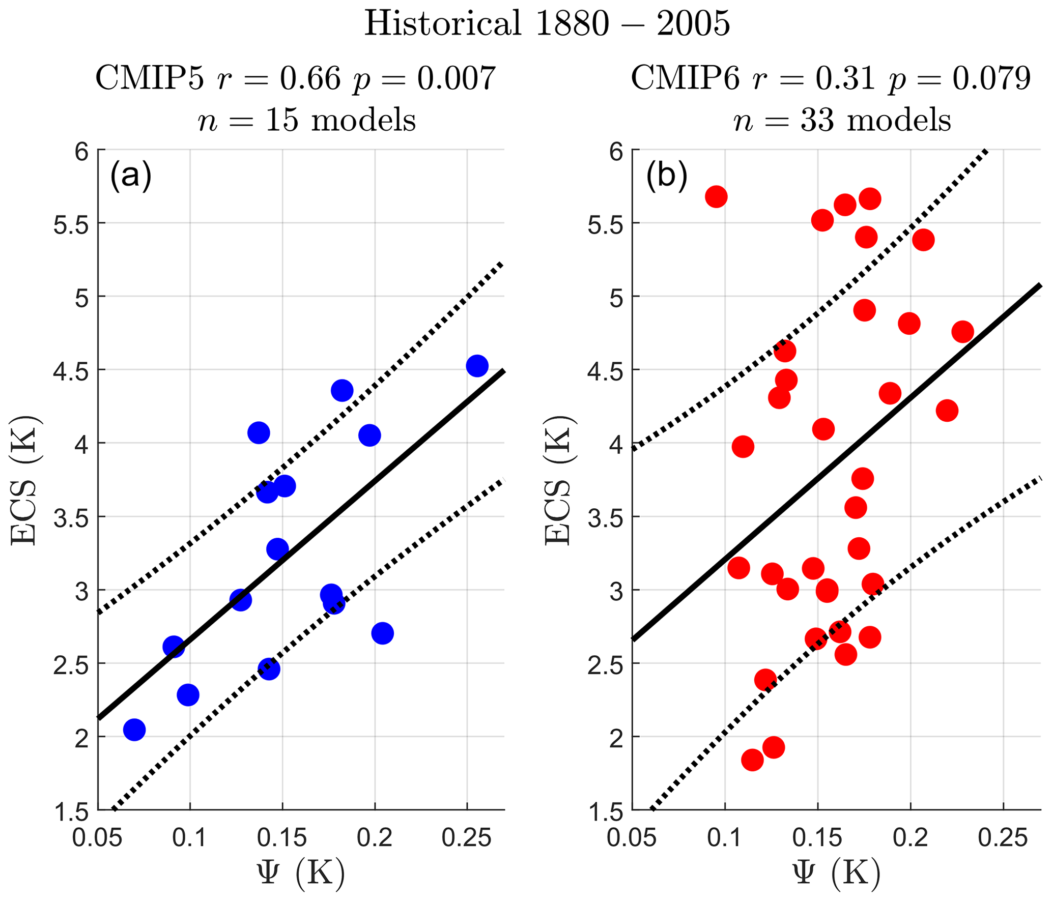
Figure 1Ψ vs. ECS emergent relationships in the CMIP5 (a) and CMIP6 (b) model ensembles running the historical experiment. The period 1880–2005 of each model's time series is used to calculate Ψ. ECS is determined from the abrupt4xCO2 experiment using the standard Gregory plot method. Individual models are plotted as circles (CMIP5 models are blue, while CMIP6 models are red). The best-fit line in the ordinary least-squares sense is shown in black along with the standard deviation of the prediction error (dotted black line). Pearson correlation r and p value are given for each emergent relationship in each subplot title.
The (Ψ, ECS) emergent relationships for CMIP5 and CMIP6 ensembles are shown in Fig. 1. The CMIP5 ensemble shows good correlation between Ψ and ECS, ; however, for CMIP6 this is weaker, , confirming the results of CHW18 (although with slightly different historical period and set of CMIP5 models) and Schlund et al. (2020) (CMIP6).
Schlund et al. (2020) use the following definitions for significance based on p value. An emergent relationship is called “highly significant” if p<0.02, “barely significant” if , “almost significant” if and “far from significant” if p≥0.1. We adopt their definitions in this paper. We find the (Ψ, ECS) emergent relationship highly significant for CMIP5 and almost significant for CMIP6.
The following assumptions are made in the CHW18 methodology to obtain the emergent relationship between Ψ and ECS.
A1. The T(t) response to Q(t) is modelled well by H76 for timescales greater than 1 year and less than the detrending window length (55 years in CHW18).
A2. H76 is solved with a random, white-noise forcing Q(t) of zero mean and standard deviation σQ. This is designed to parameterise internally generated variability (from weather, for example, Hasselmann, 1976). It is assumed that the response from all other sources of forcing in the historical period such as (but not limited to) greenhouse gases (GHGs), solar irradiance and volcanoes can be removed via detrending to a good approximation so that Eq. (2) applies to this period in both observations and CMIP models.
A3. The forcing parameters, and σQ in Eq. (2), are uncorrelated to ECS and their variation is small relative to the variation in Ψ. This requirement makes Ψ a good predictor of ECS.
There are further assumptions concerning the quantification of sources of uncertainty (structural, observational, etc.) in deriving the emergent constraint in CHW18. These are considered in more detail in Williamson and Sansom (2019) and Williamson et al. (2021). However, as we look only at the emergent relationship here, these will not discussed further.
3.1 Testing the assumptions
To summarise this subsection, assumption A3 is violated for the CMIP6 models. However, all other assumptions still apply FAPP for CMIP5 and CMIP6. In particular, it is the assumption of no correlation between ECS and the forcing parameter, σQ, that is no longer true for CMIP6. In CMIP6 significant correlation exists. Each assumption is discussed below in order.
Assumption A1 was studied in detail in Williamson et al. (2018) and Cox et al. (2018b). To summarise, H76 only really has any physical justification when the timescales of interest are dominated by the well-mixed atmosphere and ocean surface layer (a few years to decades). It is well known that H76 does a poor job of reproducing T(t) on longer timescales (e.g. Caldeira and Myhrvold, 2013; Schwartz, 2007, 2008; Foster et al., 2008; Kirk-Davidoff, 2009; Knutti et al., 2008; Scafetta, 2008). This led some to question the use of H76 in CHW18, e.g. Rypdal et al. (2018). However, one can show analytically (Williamson et al., 2018) that a near-linear emergent relationship is also expected between ECS and Ψ for the more realistic and widely used two-box (Gregory, 2000; Held et al., 2010) and diffusion models (MacMynowski et al., 2011). Both two-box and diffusion models are known to do a good job of reproducing the global annual mean temperature response of CMIP climate models (Caldeira and Myhrvold, 2013; Geoffroy et al., 2013b). As the T(t) solutions of CMIP6 models qualitatively have the same structural form as CMIP5 models to stepped and linearly increasing forcing (abrupt-4xCO2 and 1pctCO2 experiments, respectively), we expect that two-box and diffusion models also emulate the CMIP6 models well. We fit two-box models to the CMIP6 ensemble (as Geoffroy et al. (2013b) did for CMIP5) later in the paper and can confirm this is indeed the case. The reason the Ψ vs. ECS linear relationship still holds to a good degree in the more complete two-box and diffusion models is because Ψ is a statistic that is dominated by fast timescale processes of a few years, a feature H76 does capture well.
A2 assumes the response to all external forcing (GHGs, volcanoes, etc.) in the historical period can be removed to a good approximation by linearly detrending T(t) in a 55-year moving window, leaving just the internally generated random variability parameterised as the response to random “forcing” in H76.
This was the procedure introduced in CHW18, and we continue with the same procedure here for consistency and comparison. The reasons for using a 55-year window have been discussed in the original paper (Cox et al., 2018a) and subsequent publications (Cox et al., 2018b; Williamson et al., 2018). The reason for linear detrending is to remove the response due to the slow timescale in the climate. It turns out that when fitting two-box models to the CMIP models, i.e. a fast timescale (∼4 years) and a slow timescale (∼200 years) response result; see Geoffroy et al. (2013b), for example, or the tables in the Appendix B. Linear detrending with a 55-year timescale fits nicely between the short and fast timescale and removes the slow response component. It also minimises the uncertainty in the resulting emergent constraint (Cox et al., 2018a). Removing the slow timescale response leaves a signal that is more like the H76 (one-box) model and therefore more like the underlying simple theory of the emergent relationship.
Assumption A2 seeks to make the derivation of Eq. (2) (which is a derivation that applies to the piControl experiment) applicable to the historical simulations. Several works (Po-Chedley et al., 2018; Brown et al., 2018) showed this assumption to be false. In particular they showed that the detrending procedure in CHW18 does not remove the response to all external forcing. They also showed that better methods of removing forced variability slightly weakened the emergent relationship. Cox et al. (2018b) acknowledged this to be true; however, they also showed that external forcing, provided it is common for all models in the ensemble, would actually be helpful and improve the emergent relationship. This was demonstrated using an ensemble of H76 and two-box models tuned to mimic the CMIP5 models running a variety of experiments with and without common and random forcing. A sketch of the reason is as follows. Ψ is linearly proportional to sensitivity, and given an ensemble of models with a range of sensitivities, more sensitive models will respond with a larger Ψ (or response) if all models in the ensemble are given the same (common) forcing, providing a natural way of ordering the model's sensitivities. The common forcing in the historical simulations comes from volcanoes, anthropogenic trends, solar cycles, etc.
Equation (2) predicts a linear relationship between ECS and Ψ provided and σQ can be treated as “constants” across the model ensemble (assumption A3). A looser definition of constant for Eq. (2) is stated in A3. In Fig. 2a we plot against ECS and compute their correlation in both CMIP5 and CMIP6 ensembles. For both ensembles is uncorrelated to ECS ( for CMIP5, and for CMIP6; both p values, p≥0.1, are far from significant). is determined in the standard way for each model running an abrupt-4xCO2 experiment via a Gregory plot (Gregory et al., 2004).
In Fig. 2b we plot the other forcing constant σQ against ECS. σQ is estimated from the detrended temperature residual of each climate model's historical run. The standard deviation of white noise forcing σQ is fitted for each model from the global annual mean temperature time series. This time series is linearly detrended with a rolling 55 year window. This is to isolate the T(t) response to internal variability, analogous to how Ψ is determined in the CHW18 methodology, to leave the noisy T(t) response to white noise with standard deviation σT. The theoretical formula is given by (see Williamson et al., 2018 for example)
We rearrange this relation to get σQ in terms of the observable σT and the parameters λ and C (given in Tables B1, B2, B3 and B4; see Sect. 6 for details on how the H76 model parameters are fitted). Values of σQ in both the historical and piControl runs are also reported in these tables.
Consistent with CHW18, σQ is uncorrelated to ECS in CMIP5 (); however, in CMIP6 there is highly significant anti-correlation (, p<0.001). We could equally estimate σQ from piControl simulations. We choose the historical experiment for consistency with estimation of Ψ. Whichever simulation is used, the correlation with ECS remains largely invariant (piControl and in CMIP5 and CMIP6, respectively).

Figure 2Individual models are plotted as circles (CMIP5 models are blue, while CMIP6 models are red). The best-fit line in the ordinary least-squares sense is shown in black along with the standard deviation of the prediction error (dotted black line). The Pearson correlation r and p value are given for each emergent relationship in each subplot title. Shown are against CMIP5 (a) and CMIP6 (b) model ensembles. is inferred from the abrupt4xCO2 experiment using the standard Gregory plot method. σQ against ECS in the CMIP5 (c) and CMIP6 (d) model ensembles. σQ is calculated from the period 1880–2005 of each model's historical experiment time series.
When plotting the combination of constants, , multiplying Ψ in Eq. (2), (figure not shown), CMIP6 still has highly significant correlation between and ECS (r=0.74, p<0.001). CMIP5 shows some anti-correlation, although it is far from significant (, p=0.46).
We have confirmed that Ψ is a good predictor of ECS for CMIP5 models, albeit not for CMIP6 models. In Fig. 3, when σQ is included in the x-axis predictor variable, a good emergent relationship is recovered for both CMIP ensembles, and both have highly significant p values of p<0.001. One can also include (although it is uncorrelated to ECS in both CMIP ensembles) in the predictor, i.e. ECS , to get a similarly skilful emergent relationship (figure not shown). We restrict this to as minimal degrees of freedom are preferred.

Figure 3 against ECS in the CMIP5 (a) and CMIP6 (b) model ensembles running the historical experiment. The period 1880–2005 of each model's time series is used to calculate Ψ and σQ. Individual models are plotted as circles (CMIP5 models are blue, while CMIP6 models are red). The best-fit line in the ordinary least-squares sense is shown in black along with the standard deviation of the prediction error (dotted black line). Pearson correlation r and p value are given for each emergent relationship in each subplot title.
Where does the skill in predicting ECS using come from? In CMIP5, it came from Ψ (an observable). There is no skill in σQ (it is uncorrelated with ECS). In CMIP6 the converse is roughly correct. There is limited correlation with ECS from Ψ but good correlation from σQ, which, to our knowledge, is unfortunately not directly observable.
Theoretically, these findings should hold equally well in the piControl run, although the emergent relationships should have slightly weaker correlation for reasons outlined in Sect. 3.1 and Cox et al. (2018b). Again, we find this is roughly true (see Fig. 4). For the piControl experiments we analyse the longest common period simulated in the CMIP5 and CMIP6 ensembles, which is 200 years.
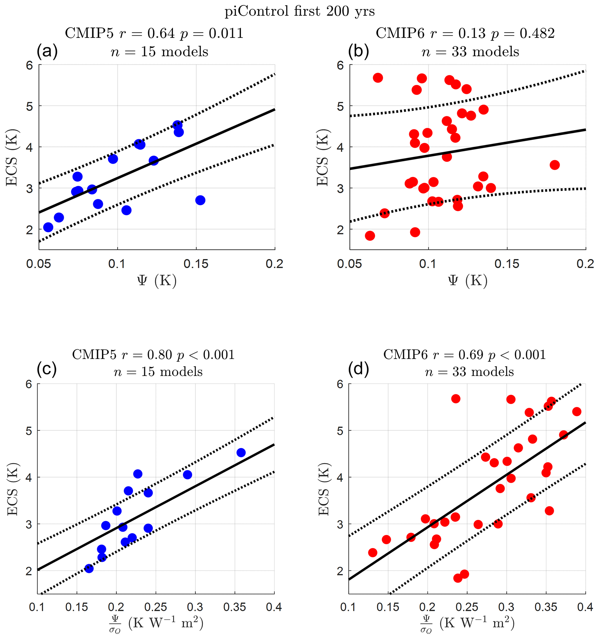
Figure 4Individual models are plotted as circles (CMIP5 models are blue and CMIP6 models are red). The best-fit line in the ordinary least-squares sense is shown in black along with the standard deviation of the prediction error (dotted black line). Pearson correlation r and p value are given for each emergent relationship in each subplot title. The first 200 years of each model's time series is used to calculate Ψ and σQ running the piControl experiment (no external forcing). (a) Ψ against ECS in the CMIP5 (a, b) and CMIP6 (c, d) model ensembles. (b) against ECS in the CMIP5 (a, b) and CMIP6 (c, d) model ensembles.
H76 in Eq. (2) predicts ECS with a constant of proportionality . We investigate the empirical value of k for the full-complexity models next. As this relation should hold for all models running any experiment (provided you can remove the forced signal), we have plotted ECS against for an ensemble composed of all CMIP5 and CMIP6 models running both piControl and historical experiments (a total of 96 data points) to determine the empirical k (Fig. 5a). While the proportionality holds with a high correlation value and significance (r=0.74, p<0.001), the empirical constant is rather than the predicted by H76, i.e. the theoretical prediction of ECS from H76 is lower than the full-complexity models suggest.
Williamson et al. (2018) showed the two-box and diffusion models also shared the linear ECS–Ψ proportionality of H76 FAPP, albeit with slightly different variables and constants. We have therefore also compared the more realistic two-box model theoretical predictions of k (Eq. 23 in Williamson et al., 2018) to the full-complexity models (Fig. 5b). Using the two-box values in Tables B5 and B6 brings the empirically determined closer to the two-box theoretical value () with similar high correlation and significance (r=0.76, p<0.001). The two-box model adds a second, longer timescale to H76, mimicking the full-complexity models more closely; however, the theoretical k is still slightly low. The lower prediction of k than the empirical results suggest this could be due to the full-complexity models having other timescales that the conceptual models do not. Although the conceptual models predict a linear ECS-Ψ proportionality also seen in the full-complexity CMIP models, they do not predict the constant of proportionality well. This is why the empirically determined k should be used to obtain an emergent constraint as in CHW18.
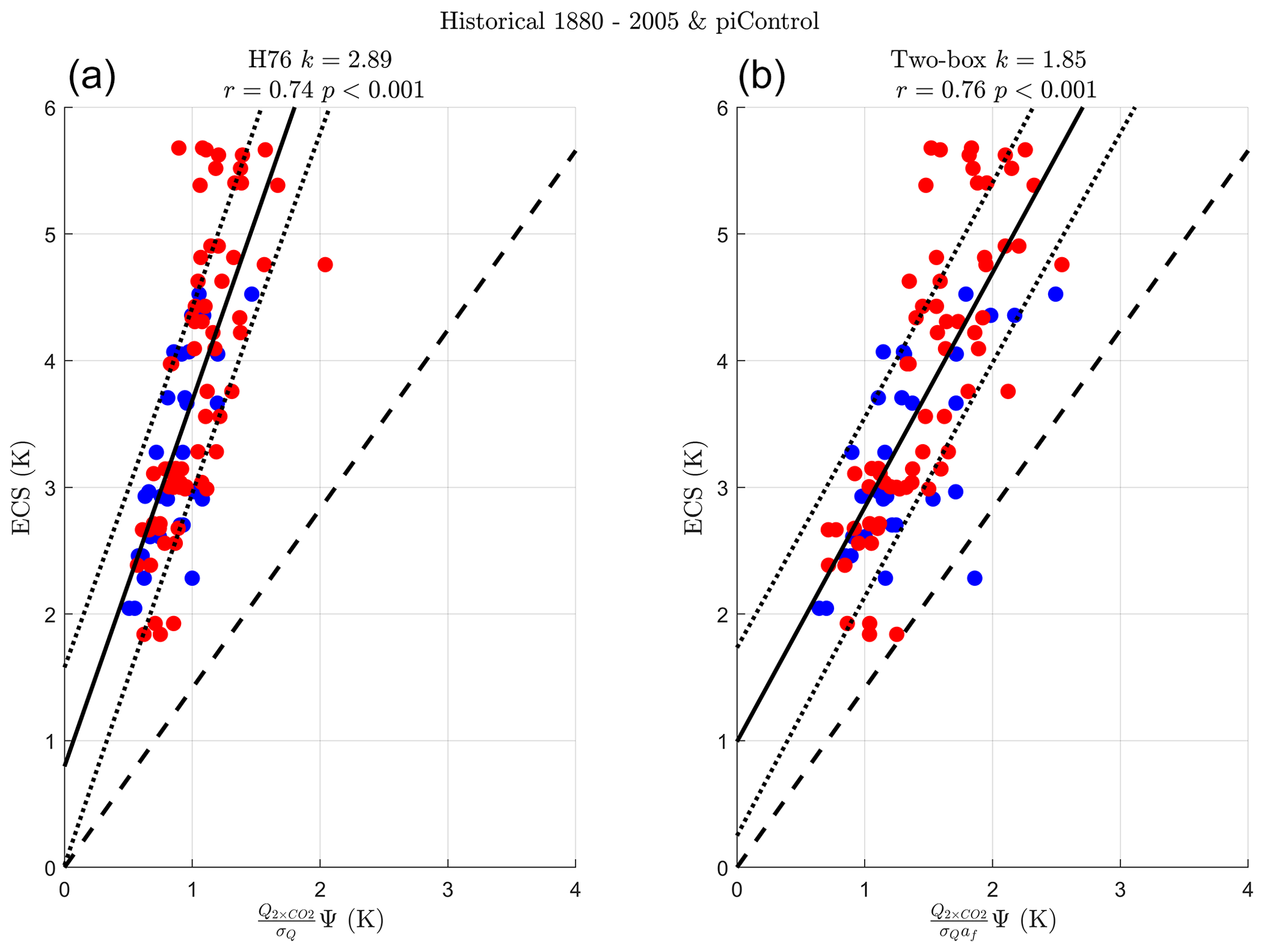
Figure 5ECS against the theoretical predictor it is proportional to in (a) the one-box or H76 model and (b) the two-box model. Individual models are plotted as circles (CMIP5 models are blue, while CMIP6 models are red) running both historical and piControl experiments between 1880–2005 and the first 200 years of the simulation respectively. The best-fit line in the ordinary least-squares sense is shown in black along with the standard deviation of the prediction error (dotted black line). Pearson correlation r and p value are given for each emergent relationship in each subplot title. The empirically determined constant of proportionality between the x-axis variable and ECS, k, is given in each subplot title. The H76 and two-box theoretical values of are plotted as the dashed black line.
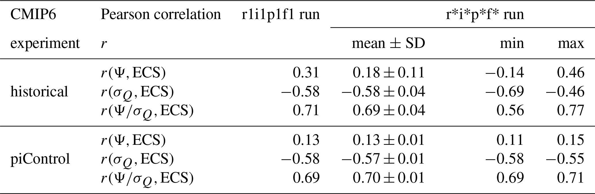
For both CMIP ensembles we have used one run for each model, preferably the one labelled or r1i1p1 (CMIP5) or r1i1p1f1 (CMIP6) where it exists; however, we could have equally chosen any r*i*p* (CMIP5) or r*i*p*f* (CMIP6) for each model provided multiple runs of the same model exist. In this section we show the results for r1i1p1 or r1i1p1f1 are representative of a typical random run choice.
For models with multiple runs, we have drawn at random one run (r*i*p* or r*i*p*f* for CMIP5 and CMIP6 respectively) for each model and repeated the analysis in the previous sections multiple times. For the historical runs, in both CMIP5 and CMIP6 ensembles, many models do repeated runs, sometimes multiple times. For example, the CMIP6 model CanESM5 has the most runs, performing the historical experiment 50 times. There are 1.6×10¹² and 5.4×10²⁰ unique permutations for the same set of CMIP5 and CMIP6 models, respectively, performing the historical experiment. These numbers are clearly too large to search exhaustively. We have therefore drawn 1000 unique permutations for the historical experiment and repeated the analysis in this paper, i.e. calculated the Pearson correlation, r, for every one of these 1000 permutations. The results are shown in the upper half of Tables 1 (CMIP5) and 2 (CMIP6). We find that the results reported for r1i1p1 and r1i1p1f1 where they exist are fairly typical of a randomly chosen set of runs; i.e. they fall within 1 standard deviation of the mean value in the CMIP5 ensemble. The CMIP6 historical experiment r(Ψ,ECS) with r1i1p1f1 is slightly higher than would be expected (mean value for a randomly chosen permutation is , far from significant, compared to r=0.31, almost significant). We have also listed the outermost values (min and max) found in the 1000 random run choice distribution for completeness. As one would expect with a large enough sample, there is a chance of finding non-representative correlations; i.e. for the CMIP5 historical ensemble there is a small possibility that you might find an (far from significant) or even (highly significant) in a random pick of runs. These are, however, not typical results.
For the piControl runs, there are 15 and 24 unique permutations for the same set of CMIP5 and CMIP6 models, respectively. The relatively low number of unique permutations is due to the low number of repeated runs for the piControl experiment. We have run the same analysis in this paper; i.e. we calculated the Pearson correlation, r, for every one of these permutations. The results are shown in the lower half of Tables 1 (CMIP5) and 2 (CMIP6). Because of the low number of unique permutations, the range of results is much narrower than the historical experiment. Again, we find that the results reported for r1i1p1 and r1i1p1f1 where they exist are fairly typical of a randomly chosen set of runs; i.e. they fall within 1 standard deviation of the mean value in the CMIP5 and CMIP6 ensembles with the exception of CMIP5 (highly significant) for r1i1p1 compared to (highly significant) for a randomly chosen permutation. This is actually the highest value of r (max) found in that experiment.
Table 1Details of the CMIP5 experiment showing the robustness of correlation to choice of run, including a comparison of Pearson correlation r for model ensembles using the r1i1p1 run (third column) with randomly chosen runs r*i*p*. There are 15 unique permutations of runs for the piControl experiment and 1.6×10¹² unique permutations for the historical experiment. We calculate r for all unique permutations for the piControl experiment and 1000 randomly chosen unique permutations for the historical experiment. We report the mean value of r with its standard deviation (±) in the fourth column and the most extreme values of r in the fifth and sixth columns.
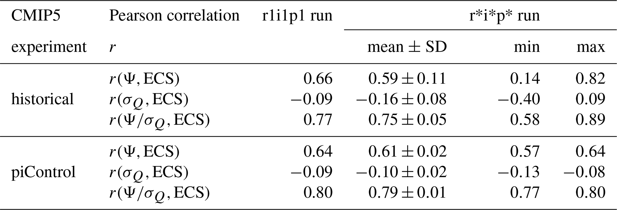
Table 2Details of the CMIP6 experiment showing the robustness of correlation to choice of run, including a comparison of Pearson correlation r for model ensemble using the r1i1p1f1 run if available (third column) with randomly chosen runs r*i*p*f*. There are 24 unique permutations of runs for the piControl experiment and 5.4×10²⁰ unique permutations for the historical experiment. We calculate r for all unique permutations for the piControl experiment and 1000 randomly chosen unique permutations for the historical experiment. We report the mean value of r with its standard deviation (±) in the fourth column and the most extreme values of r in the fifth and sixth columns.
In Sect. 4 we found that by including the forcing parameter σQ in the predictor for ECS an emergent relationship could be recovered for both CMIP5 and CMIP6 ensembles. These relationships are present in both the historical and piControl experiments, giving confidence in the underlying theoretical basis FAPP.
In this section we make a more demanding test of the theoretical basis by asking if theory alone can simulate the full-complexity CMIP model ensemble r(Ψ,ECS) and results. To do this, we create a H76 model emulator of each of the full-complexity CMIP5 and CMIP6 models used in the preceding figures. With the emulator H76 models we can build emulator H76 CMIP5 and CMIP6 ensembles and run analogous historical and piControl experiments with them. This will allow us to compare the results of the pure theory used in CHW18 with that of the full-complexity CMIP model ensembles. We also fit the more complete two-box model in addition for comparison (see Sect. A).
6.1 Methodology
The H76 model fitted to each of the full-complexity CMIP models is given by Eq. (1). Parameters are fitted from the full-complexity abrupt-4xCO2 CMIP model experiments: λ and are determined from Gregory plots (Tables B1, B2), C is found using a modification of the methodology of Geoffroy et al. (2013b) (Tables B3 and B4). Geoffroy et al. (2013b) published parameter values for two-box models fitted to CMIP5 models. The two-box model is H76's well-mixed upper-ocean and atmosphere box extended by coupling it to a large heat capacity deep-ocean box (see Sect. A). This gives the two-box model a fast and a slow e-folding timescale of adjustment with typical values of ∼4 and ∼200 years when fitted to CMIP models (see Geoffroy et al., 2013b and Tables B5 and B6), which is known to do a good job reproducing the global annual mean temperature response of climate models.
As H76 only has one box and therefore one timescale, it cannot capture both fast and slow responses of CMIP models. Because Ψ is a statistic that is dominated by fast timescale processes of a few years, a feature H76 does capture well, we choose to fit the fast response with H76 using the fast timescale fitting methodology of Geoffroy et al. (2013b) (see Eq. 18 in that paper). When modified for H76, this equation becomes
We fit H76's timescale parameter (and therefore the heat capacity C) by averaging over the first 5 years of the abrupt-4xCO2 experiment. We choose the average over 5 years rather than the first 10 in the two-box fits of Geoffroy et al. (2013b). This is because the H76 fit gets worse as the number of years in the average increases (in the root-mean-square error of the fit). For the two-box fits we use the methodology of Geoffroy et al. (2013b) unmodified (see Sect. A for complete details).
Fitted values of λ, τ, C and σQ are reported for CMIP5 and CMIP6 ensembles in Tables B3 and B4 respectively.
6.2 Emulator piControl experiments
We perform analogous piControl experiments with the H76 and two-box CMIP5 and CMIP6 ensembles by integrating each of the individual CMIP H76 (and two-box) emulators (Eqs. 1 and A1 respectively) numerically with forcing Qi(t), a zero mean random variable with model specific standard deviation σQi and Gaussian pdf. We write this as
where ηi(t) is the Gaussian random variable with unit standard deviation. The equations are integrated with a time step of 0.1 years using the Euler–Maruyama method. The Ti(t) time series that result are then analysed in the same way as the full-complexity CMIP model time series to produce a pair of values (Ψi,ECSi). For the full set of n two-box models in each CMIP emulator ensemble r(Ψ,ECS) and are calculated. Because Qi(t) is a random variable of finite length, repeating the same experiment results in slightly different values of for each run due to the properties of statistical estimators (estimation converges as where N is the number of points in the time series). The same applies to different initial value runs in the full-complexity models due to the chaotic weather variability the random forcing captures in the H76 and two-box models. We therefore repeat each piControl emulator experiment 250 times and compare the distribution of emulator r(Ψ,ECS) values with the single full-complexity CMIP piControl experiment.
Results are shown in Fig. 6. Agreement between the H76 emulator CMIP r(Ψ,ECS) and the full-complexity CMIP ensembles is reasonable. Full-complexity CMIP5 ensemble r(Ψ,ECS) results (Fig. 6a, dotted blue line) fall in the upper end of the distribution of r(Ψ,ECS) H76 emulator values. Although full-complexity r(Ψ,ECS) CMIP6 results (in red) were shown to be lower in correlation (red dotted line), they can still be simulated reasonably well by the H76 emulator ensemble, falling like CMIP5, in upper end of simulated r(Ψ,ECS) values. In Fig. 6b where Ψ is now normalised by the mean amplitude of the random forcing σQ both CMIP5 and CMIP6 results are much more similar, with histograms of the H76 emulator ensembles and the full-complexity results having much more overlap, although simulated values are still on average slightly lower than the full-complexity ensembles.
Analogous figures simulated with two-box emulator CMIP ensembles are shown in Fig. A1. The two-box ensembles do an even better job of simulating the full-complexity CMIP results.
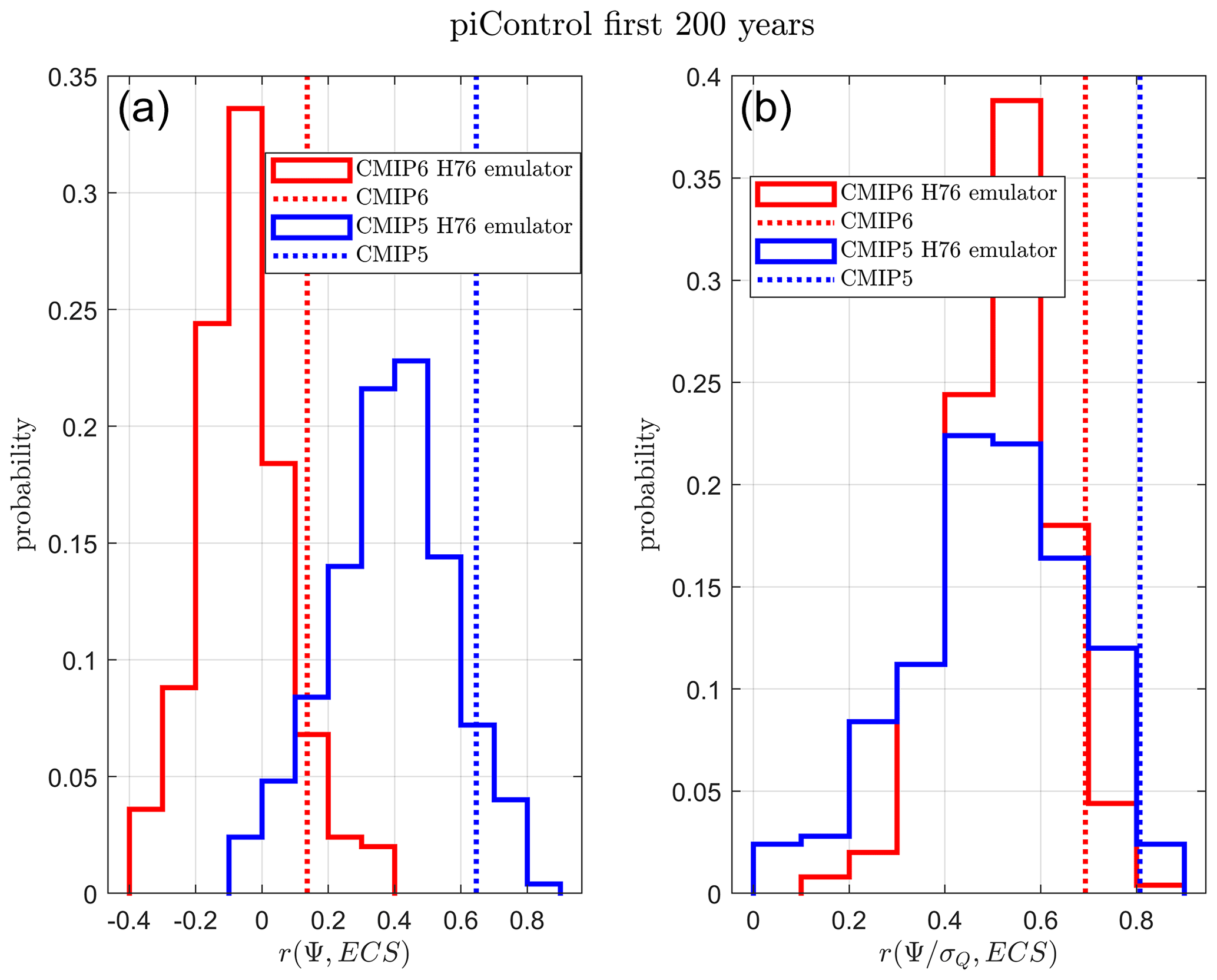
Figure 6Probability of obtaining r(Ψ,ECS) (a) and (b) in the H76 CMIP emulator ensembles performing a piControl simulation of 200 years. The CMIP5 emulator ensemble histogram is given in blue, and the equivalent data for CMIP6 are shown in red. The full-complexity CMIP ensemble results performing the same experiment are shown as vertical dotted lines.
6.3 Emulator historical experiments
The analogous historical experiments are performed in the same way to the piControl experiments but with a common external forcing component Qi(t) in addition to the random forcing. This comes from GHGs, volcanoes, solar cycles and others. For this common external forcing component we use Meinshausen et al. (2011) reconstructed historical forcing (QIPCC(t)). Explicitly, this is written as
in the historical simulations. We integrate the H76 and two-box ensembles between the years 1765 and 2005 but calculate Ψ and r(Ψ,ECS) between 1880–2005 to correspond to the full-complexity model analysis. Results are shown in Fig. 7. As with the piControl experiments in Sect. 6.2, agreement between the pure-theory H76 emulator ensembles and the full-complexity ensembles is reasonable, giving confidence that the underlying theory used in CHW18 is good FAPP. The analogous figure simulated with two-box CMIP emulator ensembles does an even better job (Fig. A2).
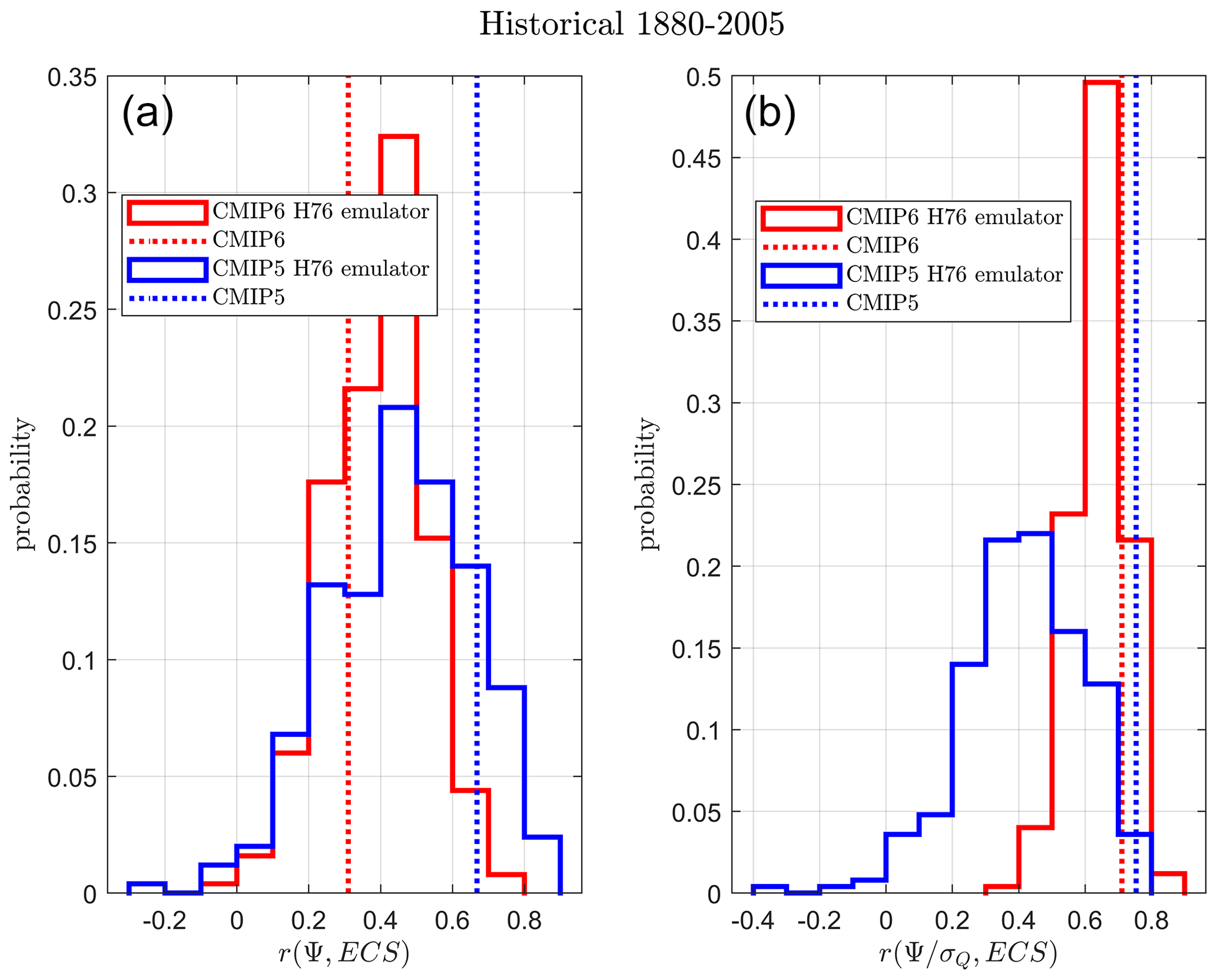
Figure 7Probability of obtaining r(Ψ,ECS) (a) and (b) in the H76 CMIP emulator ensembles performing a historical simulation of the period 1880–2005. The CMIP5 emulator ensemble histogram is given in blue, and the equivalent data for CMIP6 are shown in red. The full-complexity CMIP ensemble results performing the same experiment are shown as vertical dotted lines.
6.4 Emulator experiments with constant σQ
We have shown that by taking into account model-specific σQ in the CHW18 theory we can both understand r(Ψ,ECS) correlation results and can recover good emergent relationships for both CMIP5 and CMIP6 in piControl and historical runs. In CHW18 and Cox et al. (2018b) it was assumed that σQ was constant for each model in the CMIP5 ensemble (assumption A3). We now test this assumption with the H76 and two-box CMIP ensembles. Instead of fitting σQ to each CMIP model we fix it to be a constant, σQ=0.25 W m−2 following Cox et al. (2018b). This value was chosen (even though it is lower than the values given in the tables) as it was the mean value of the standard deviation of net top-of-the-atmosphere radiation, which was thought to be a good proxy for σQ at that time. Results with constant, model-independent σQ for r(Ψ,ECS) are shown in Figs. 8 (H76) and A3 (two-box) for both piControl and historical experiments. results are not shown as they are identical to r(Ψ,ECS). This is because the predictors, the set of {Ψi}, are all divided by the same constant.
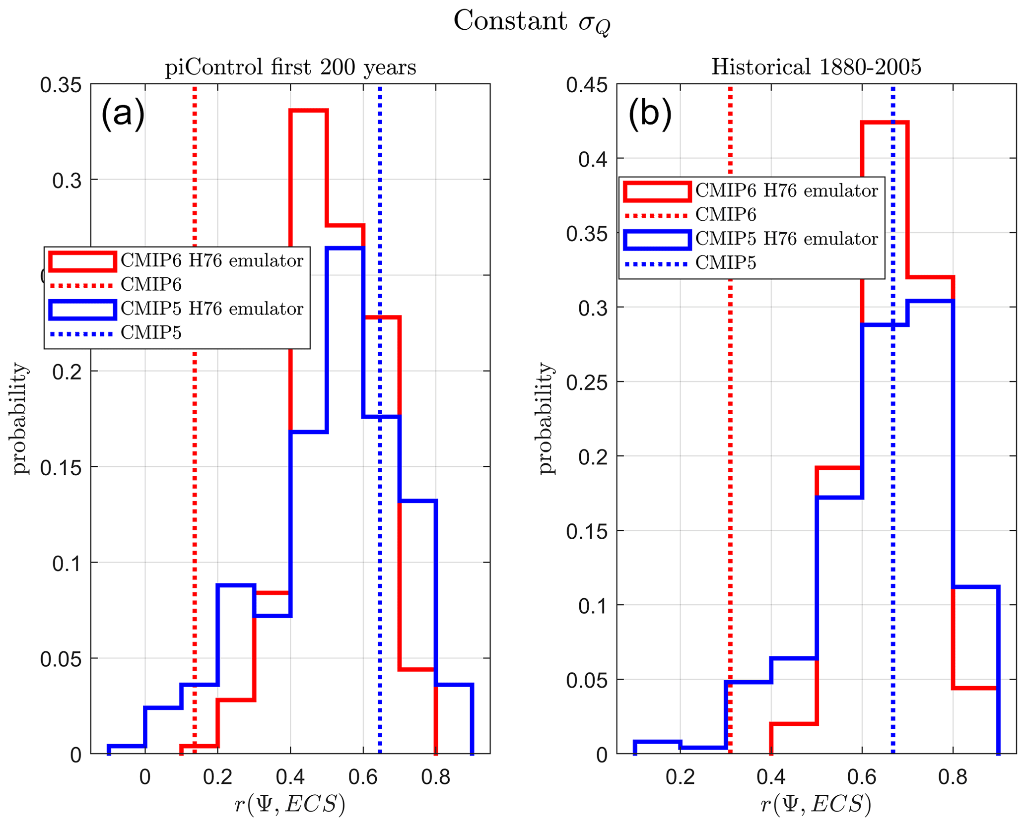
Figure 8Probability of obtaining r(Ψ,ECS) in the H76 CMIP emulator ensembles performing a piControl (a) and historical (b) simulation if each two-box emulator is given the same value of σQ=0.25 W m−2. The CMIP5 emulator ensemble histogram is given in blue, and the equivalent data for CMIP6 are shown in red. The full-complexity CMIP ensemble results performing the same experiment are shown as vertical dotted lines.
The constant σQ assumption can be seen to be good for the CMIP5 ensemble (blue) with full-complexity models (dotted blue line) agreeing well with likely values of the H76 and two-box CMIP5 emulator ensembles (blue histogram). However, the full-complexity CMIP6 ensemble (dotted red line) correlations are generally much lower than the CMIP6 emulators (red histogram). This is again supporting evidence that the underlying theory in CHW18 is sound FAPP. The similarity in the CMIP5 and CMIP6 histograms also suggests there is no real difference in the parameters of the emulator ensembles. The difference can be attributed to the amount of correlation between σQ and ECS in the CMIP5 and CMIP6 ensembles.
The aim of this paper was to understand why the strong emergent relationship from CHW18 found in the CMIP5 model ensemble weakened in the newer CMIP6 ensemble. This emergent relationship was based on reasonable, albeit simple, physical principles, and thus it is interesting (and important) to understand the differences between the theory and full-complexity models. A number of assumptions (Sect. 3) were made in deriving the theoretical emergent relationship between the predictor Ψ, a metric based on annual global mean temperature variability and ECS, the predictand in CHW18. We have shown the “no correlation between forcing and ECS” assumption no longer holds for the CMIP6 ensemble. In particular, the parameter σQ describing random forcing from internally generated variability, is correlated to ECS in CMIP6, and when this parameter is incorporated into the predictand, a good emergent relationship is recovered for both CMIP ensembles.
Assumption A3 stated that the forcing parameters, and σQ, could be treated as constants across a model ensemble. While this is a fair assumption for for both CMIP ensembles and σQ in the CMIP5 ensemble, we have shown that σQ is correlated to ECS in the CMIP6 ensemble. We have also shown that when the predictor of ECS is changed to , good emergent relationships are recovered in both CMIP ensembles for both piControl and historical experiments. We also showed that pure theory could reproduce the full-complexity CMIP model results using H76 and two-box CMIP emulator ensembles. Although the proportionality between ECS and the predictor has a high correlation and significance, simple pure theory underestimates the constant of proportionality. Aside from this, these results give us confidence the theoretical basis of CHW18 still applies to CMIP6 models as it did for CMIP5 FAPP. Testing the theoretical basis was the underlying aim of our study.
However, several questions remain. Can we estimate σQ from observations and therefore get an emergent constraint on ECS from the CMIP6 ensemble? Why is σQ correlated to ECS in CMIP6 and not CMIP5? σQ is a parameter designed to reproduce the observed global annual mean temperature variability, σT, in the non-chaotic H76 and two-box models. In the full-complexity models and the real world, this parameter attempts to capture chaotic internal variability and sub-annual (fast) feedbacks. It is fitted in this study using σT (an observable) as well as the unobservable two-box parameters. The reliance on these unobservable two-box parameters makes it appear that getting an estimate of σQ in the real world and thus an emergent constraint may be tough. However, there may be observable proxies for σQ that we have not yet found.
An obvious place to start looking for a proxy for σQ is in basic theory. The simplest example that one can imagine is
where N(t) is the net top-of-the-atmosphere radiative flux. However this still requires knowledge of λ. Even given knowledge of λ it is well known (Forster, 2016) that N is poorly correlated to T where most of the change in N and T is driven by internal variability (although this relation works very well for large forced trends; e.g. the Gregory method works well applied to large stepped increases in CO2). There are several models (Winton et al., 2010; Geoffroy et al., 2013a) and methods (Dessler et al., 2018; Bloch-Johnson et al., 2020) that get much better correlations between N and T when most of the changes are driven internally by taking into account the spatial distributions (the so-called pattern effect; see Armour et al., 2012). We leave this to a future study.
The question of why σQ is correlated to ECS in CMIP6 and not CMIP5 is also left unanswered. However, one can speculate why this may be the case. As previously mentioned σQ is a fitting parameter that is designed to capture the effect of chaotic internal variability and sub-annual (fast) feedbacks on global mean temperature variability. Zelinka et al. (2020) showed that the increased range of ECS in the CMIP6 models could be explained by the increased range in cloud feedbacks (see also Bock and Lauer, 2024). As σQ is fitted to annual temperature time series, some of this fast (sub-annual) cloud feedback effect could be included in σQ, correlating it to ECS. We leave concrete answers to a future study.
We have understood what assumption in the theoretical emergent relationship for CHW18 was responsible for the weakened correlation in CMIP6, namely that σQ is correlated with ECS. When accounted for, good emergent relationships are recovered. Although the information that the simple theory holds FAPP is useful and that σQ is correlated in CMIP6 with ECS is interesting, it is disappointingly not useful in constraining ECS due to the unobservable nature (we think) of σQ. In this sense, the method in CHW18 does not produce a useful emergent constraint on CMIP6 because the extra degree of freedom in σQ needs to be incorporated.
Schlund et al. (2020) tested 11 emergent constraints found in CMIP5, and nearly all of these got weaker in CMIP6. We do not know whether they failed for similar reasons. Indeed, many of them do not have a simple theoretical model as a basis for their emergent relationship, which means that assumption testing, the approach we follow in this paper, would be difficult to do. This is why we argue that emergent constraints should be based on a testable, falsifiable theoretical model. This aids understanding and lifts emergent constraint research from looking for strong correlations between variables to a more scientific approach of testing hypotheses of how the Earth system works. However, looking at all these other emergent constraints and identifying why they got weaker in CMIP6 would be very beneficial to understanding and useful to the community.
Emergent constraints based on theory with minimal degrees of freedom are most likely to be the most robust and useful. Constraints such as Hall and Qu (2006) on snow albedo feedback where the predictor (seasonal cycle snow albedo feedback) and predictand (climate change snow albedo feedback) are the essentially the same variable have been shown to be robust through three CMIP generations (Thackeray et al., 2021). Other constraints of this type that are likely to be more robust are the transient climate response constraints of Nijsse et al. (2020) and Tokarska et al. (2020) where near-term historical warming is the predictor of future longer-term warming.
Even if emergent relationships based on sound theoretical principles do fail there is still information to be gleaned on understanding why. Today, there is even more of an opportunity for the top-down insights of specific conceptual models to meet and complement the comprehensive, bottom-up approach from state-of-the-art climate models; there are many more high-quality observations; the global warming signal has also become clearer over time; and there is also a large archive of past and present climate model simulations.
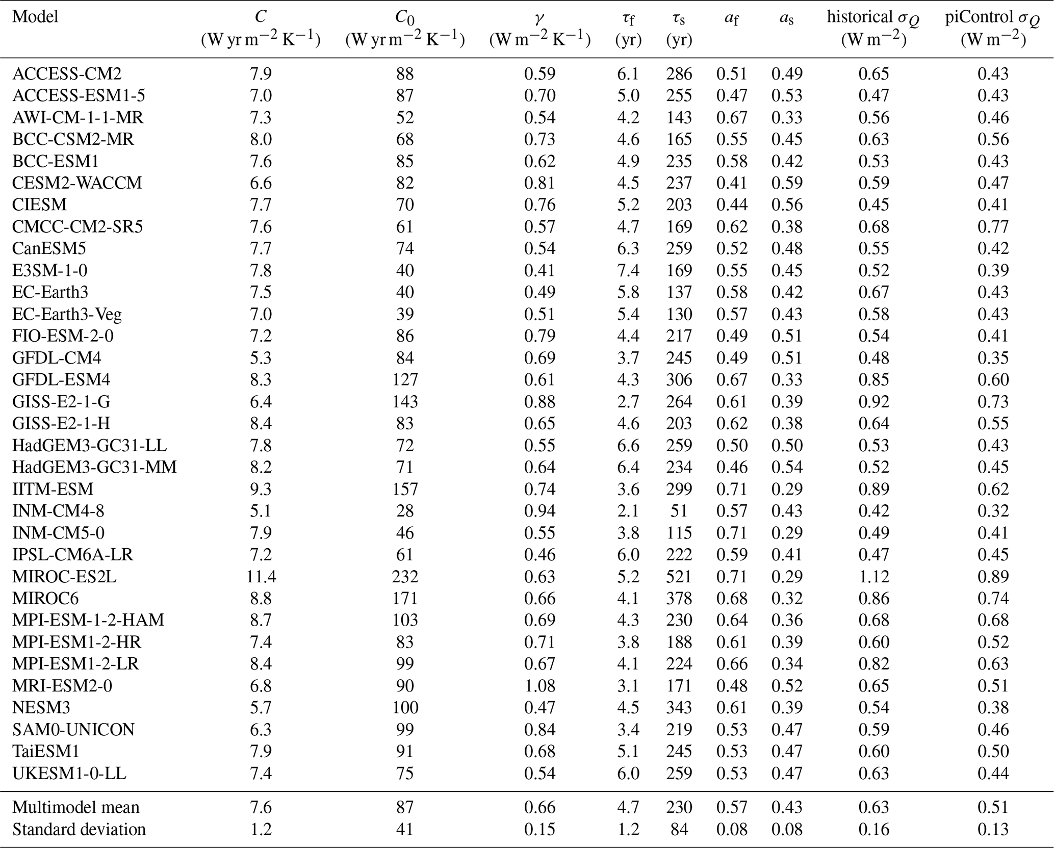
The two-box model is H76's low thermal inertia atmosphere and well-mixed ocean surface layer with heat capacity C extended with a large-heat-capacity C0 deep-ocean box coupled to the surface box by flux γ. This gives the model two timescales of adjustment, a fast (τf) and a slow e-folding time (τs). When fitted to CMIP models, typical values for the timescales are τf∼4 years and τs∼200 years (see Tables B5 and B6).
Each CMIP model labelled with i is “mimicked” by the two-box equations
T0i is the annual global-mean deep-ocean temperature anomaly of model i. Parameters are fitted from the full-complexity abrupt-4xCO2 CMIP model experiments. The parameters λ and are determined from Gregory plots, while C, C0 and γ are determined using Geoffroy's methodology (Geoffroy et al., 2013b). We use the published values of Geoffroy et al. (2013b) for CMIP5 models. Values for CMIP6 models are given in Tables B2 and B6.
The standard deviation of white-noise forcing σQ is fitted for each model from the global annual mean temperature time series of either the piControl or historical experiment. This time series is linearly detrended with a rolling 55-year window. This is to isolate the T(t) response to internal variability, analogous to how Ψ is determined in the CHW18 methodology, to leave the noisy T(t) response to white noise with standard deviation σT. The theoretical formula is given by Williamson et al. (2018)
We rearrange this relation to get σQ. Values of λ, af, as, τf and τs are taken from Tables B1, B2, B5 and B6. Values of σQ in both historical and piControl runs are also reported in Tables B5 and B6. The parameters af, as, τf and τs are complicated functions of the parameters C, C0, λ and γ. Their exact full functional forms can be found in Geoffroy et al. (2013b) and are not given here.
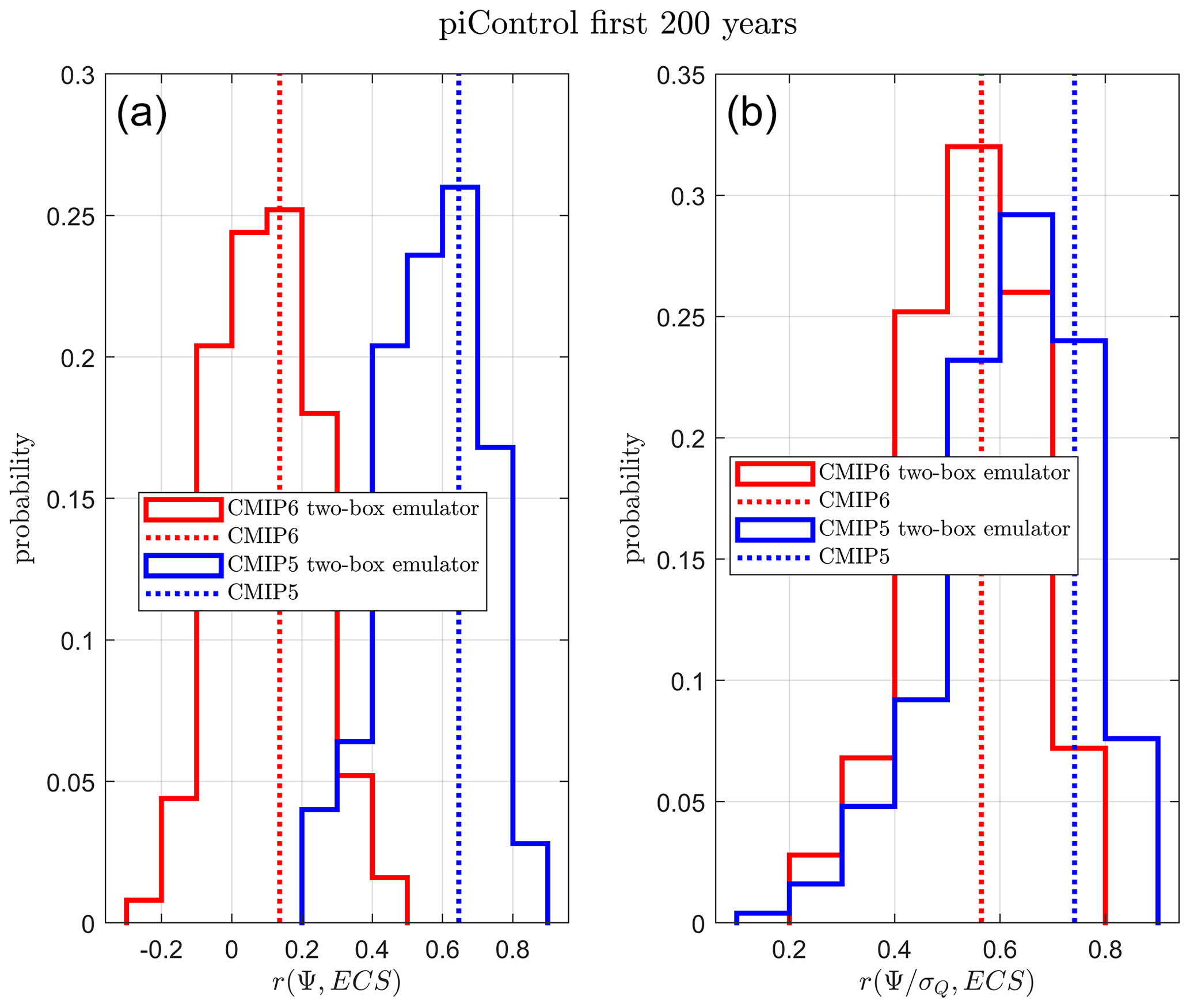
Figure A1Probability of obtaining r(Ψ,ECS) (a) and (b) in the two-box CMIP emulator ensembles performing a piControl simulation of 200 years. The CMIP5 emulator ensemble histogram is given in blue, and the equivalent data for CMIP6 are shown in red. The full-complexity CMIP ensemble results performing the same experiment are shown as vertical dotted lines.

Figure A2Probability of obtaining r(Ψ,ECS) (a) and (b) in the two-box CMIP emulator ensembles performing a historical simulation of the period 1880–2005. The CMIP5 emulator ensemble histogram is given in blue, and the equivalent data for CMIP6 are shown in red. The full-complexity CMIP ensemble results performing the same experiment are shown as vertical dotted lines.
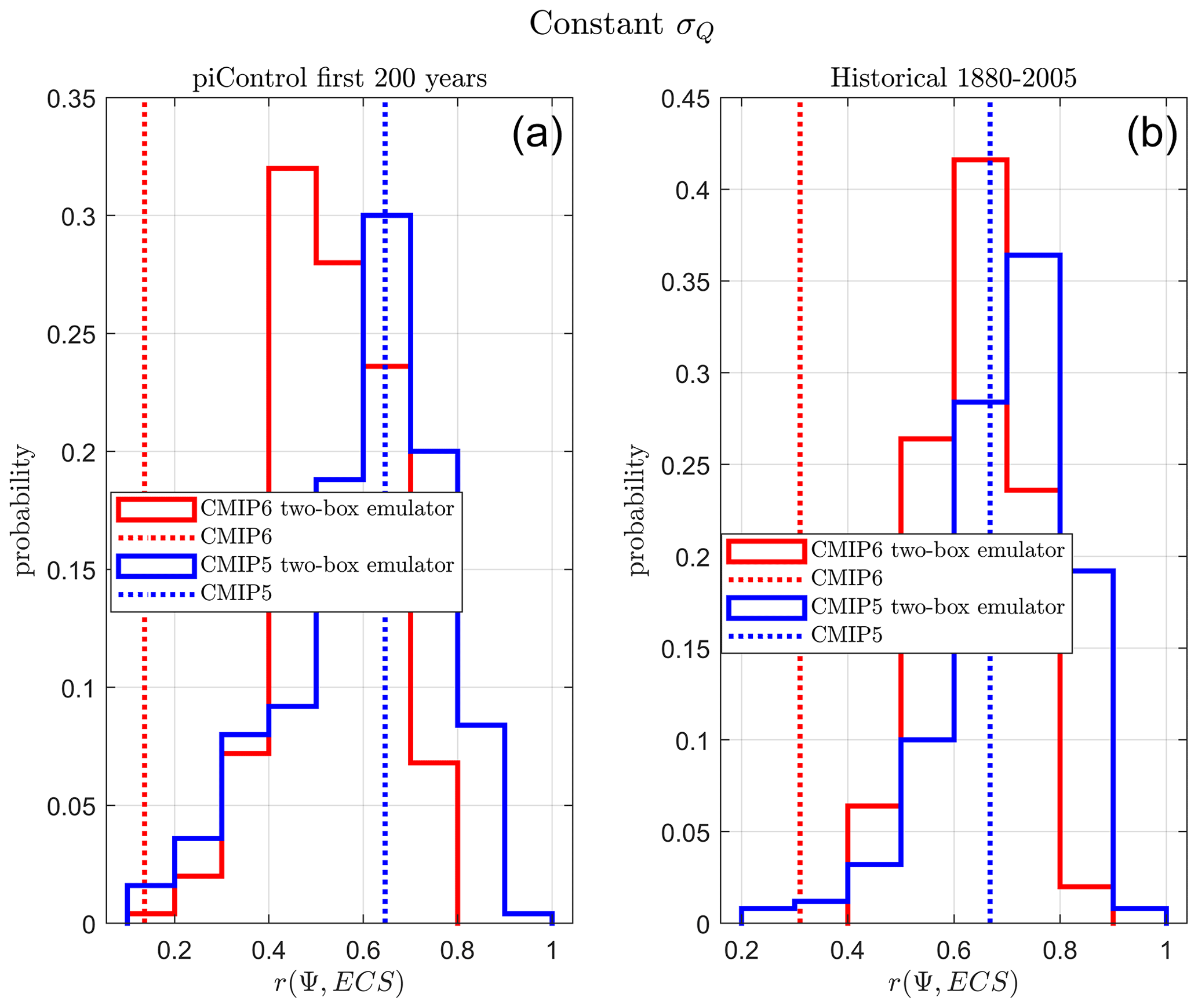
Figure A3Probability of obtaining r(Ψ,ECS) in the two-box CMIP emulator ensembles performing a piControl (a) and historical (b) simulation if each two-box emulator is given the same value of σQ=0.25 W m−2. The CMIP5 emulator ensemble histogram is given in blue, and the equivalent data for CMIP6 are shown in red. The full-complexity CMIP ensemble results performing the same experiment are shown as vertical dotted lines.
Table B1Gregory plot determined parameters for CMIP5 models from Geoffroy et al. (2013b).
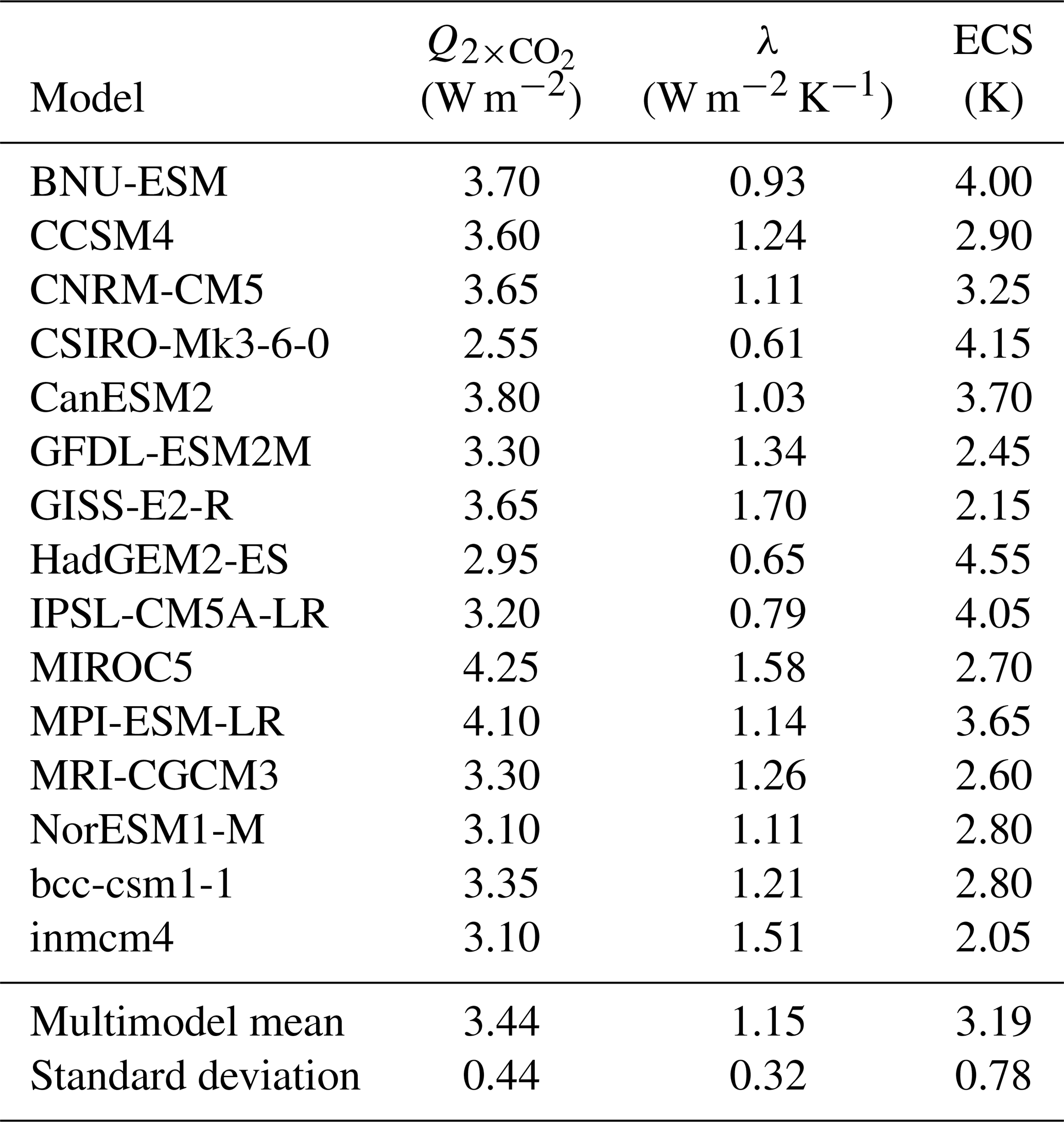
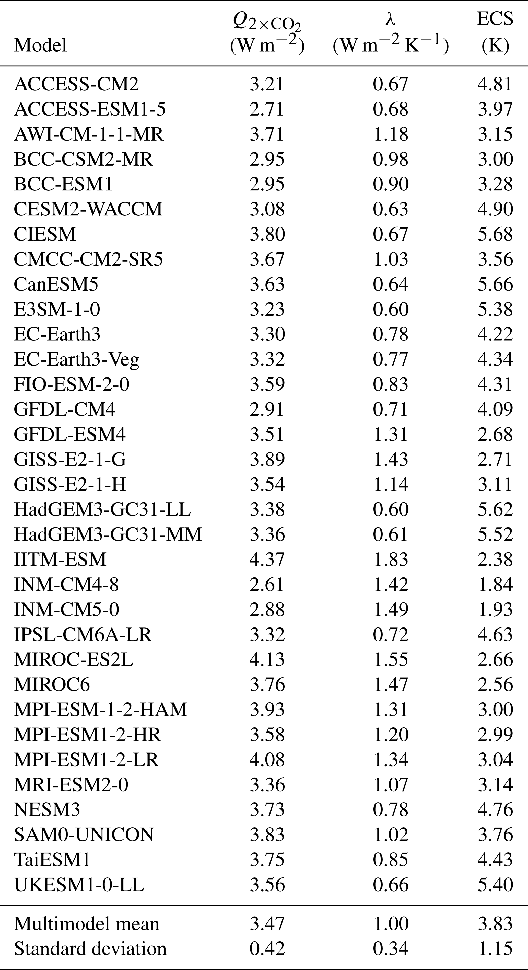
Table B3H76 model parameters fitted from abrupt4xCO2 runs for CMIP5 models. The σQ values are calculated from detrended T(t) for either historical or piControl runs.
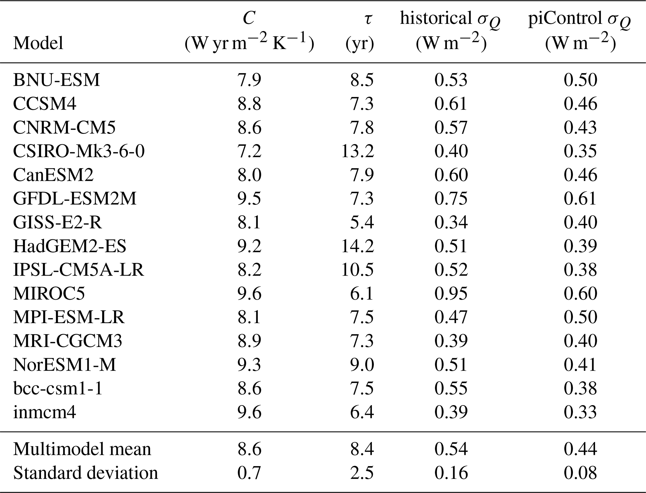
Table B4H76 model parameters fitted from abrupt4xCO2 runs for CMIP6 models. The σQ values are calculated from detrended T(t) for either historical or piControl runs.
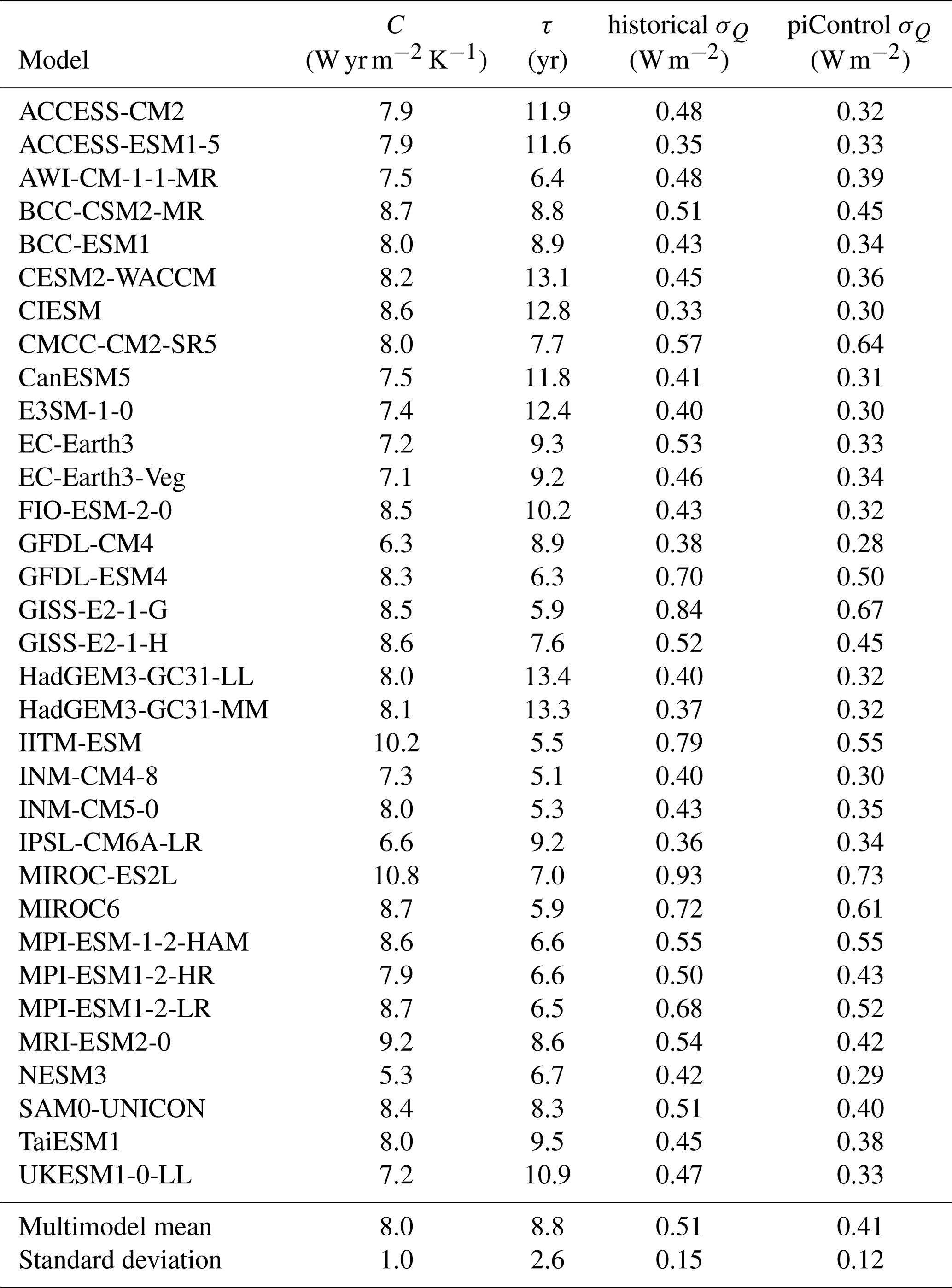
Table B5Two-box parameters fitted from abrupt4xCO2 runs for CMIP5 models taken from Geoffroy et al. (2013b). The σQ values are calculated from detrended T(t) for either historical or piControl runs.

Table B6Two-box parameters fitted from abrupt4xCO2 runs for CMIP6 models. The σQ values are calculated from detrended T(t) for either historical or piControl runs.
All original CMIP5 and CMIP6 data used in this study are publicly available at https://esgf-node.llnl.gov/projects/cmip5/ (CMIP5_database, 2021) and https://esgf-node.llnl.gov/projects/cmip6/ (CMIP6_database, 2021), respectively.
MSW carried out the data analysis and drafted the paper with advice from PMC, CH and FJMMN. All authors contributed to the submitted paper.
The contact author has declared that none of the authors has any competing interests.
Publisher’s note: Copernicus Publications remains neutral with regard to jurisdictional claims made in the text, published maps, institutional affiliations, or any other geographical representation in this paper. While Copernicus Publications makes every effort to include appropriate place names, the final responsibility lies with the authors.
This work was supported by the European Research Council (ERC) ECCLES project, grant agreement no. 742472 (Mark S. Williamson, Peter M. Cox and Femke J. M. M. Nijsse); the EU Horizon 2020 Research Programme CRESCENDO project, grant agreement no. 641816 (Mark S. Williamson and Peter M. Cox); the Horizon Europe project OptimESM, grant agreement no. 101081193 (Peter M. Cox); and the NERC UKCEH National Capability fund (Chris Huntingford). We also acknowledge the World Climate Research Programme's Working Group on Coupled Modelling, which is responsible for CMIP, and we thank the climate modelling groups for producing and making their model output available.
This research has been supported by the HORIZON European Research Council (grant nos. 742472 and 641816), the Horizon Europe project OptimESM (grant no. 101081193), and the NERC UKCEH National Capability fund.
This paper was edited by Roberta D'Agostino and reviewed by BB Cael and two anonymous referees.
Armour, K. C., Bitz, C. M., and Roe, G. H.: Time-Varying Climate Sensitivity from Regional Feedbacks, J. Climate, 26, 4518–4534, https://doi.org/10.1175/JCLI-D-12-00544.1, 2012. a
Bell, J.: Against “measurement”, Physics World, 3, 33, https://doi.org/10.1088/2058-7058/3/8/26, 1990. a
Bloch-Johnson, J., Rugenstein, M., and Abbot, D. S.: Spatial Radiative Feedbacks from Internal Variability Using Multiple Regression, J. Climate, 33, 4121–4140, https://doi.org/10.1175/JCLI-D-19-0396.1, 2020. a
Bock, L. and Lauer, A.: Cloud properties and their projected changes in CMIP models with low to high climate sensitivity, Atmos. Chem. Phys., 24, 1587–1605, https://doi.org/10.5194/acp-24-1587-2024, 2024. a
Bracegirdle, T. J. and Stephenson, D. B.: On the robustness of emergent constraints used in multimodel climate change projections of Arctic warming, J. Climate, 26, 669–678, https://doi.org/10.1175/JCLI-D-12-00537.1, 2013. a
Brient, F.: Reducing Uncertainties in Climate Projections with Emergent Constraints: Concepts, Examples and Prospects, Adv. Atmos. Sci., 37, 1–15, https://doi.org/10.1007/s00376-019-9140-8, 2020. a
Brown, P. T., Stolpe, M. B., and Caldeira, K.: Assumptions for emergent constraints, Nature, 563, E1–E3, https://doi.org/10.1038/s41586-018-0638-5, 2018. a, b
Caldeira, K. and Myhrvold, N. P.: Projections of the pace of warming following an abrupt increase in atmospheric carbon dioxide concentration, Environ. Res. Lett., 8, 034039, https://doi.org/10.1088/1748-9326/8/3/034039, 2013. a, b, c
Caldwell, P. M., Bretherton, C. S., Zelinka, M. D., Klein, S. A., Santer, B. D., and Sanderson, B. M.: Statistical significance of climate sensitivity predictors obtained by data mining, Geophys. Res. Lett., 41, 1803–1808, https://doi.org/10.1002/2014GL059205, 2014. a
Caldwell, P. M., Zelinka, M. D., and Klein, S. A.: Evaluating Emergent Constraints on Equilibrium Climate Sensitivity, J. Climate, 31, 3921–3942, https://doi.org/10.1175/jcli-d-17-0631.1, 2018. a
CMIP5_database: The Climate Model Intercomparison Project version 5 data ensemble, Earth System Grid Federation portal [data set], https://esgf-node.llnl.gov/projects/cmip5/ (last access: August 2021), 2021.
CMIP6_database: The Climate Model Intercomparison Project version 6 data ensemble, Earth System Grid Federation portal [data set], https://esgf-node.llnl.gov/projects/cmip6/ (last access: August 2021), 2021.
Covey, C., Guilyardi, E., Jiang, X., Johns, T. C., Treut, H. L., Madec, G., Meehl, G. A., Miller, R., Power, S. B., Roeckner, E., and Russell, G.: The seasonal cycle in coupled ocean-atmosphere general circulation models, Clim. Dynam., 16, 775–787, 2000. a
Cox, P. M., Huntingford, C., and Williamson, M. S.: Emergent constraint on equilibrium climate sensitivity from global temperature variability, Nature, 553, 319, https://doi.org/10.1038/nature25450, 2018a. a, b, c, d
Cox, P. M., Williamson, M. S., Nijsse, F. J. M. M., and Huntingford, C.: Cox et al. reply, Nature, 563, E10–E15, https://doi.org/10.1038/s41586-018-0641-x, 2018b. a, b, c, d, e, f, g
Dessler, A. E., Mauritsen, T., and Stevens, B.: The influence of internal variability on Earth's energy balance framework and implications for estimating climate sensitivity, Atmos. Chem. Phys., 18, 5147–5155, https://doi.org/10.5194/acp-18-5147-2018, 2018. a
Eyring, V., Bony, S., Meehl, G. A., Senior, C. A., Stevens, B., Stouffer, R. J., and Taylor, K. E.: Overview of the Coupled Model Intercomparison Project Phase 6 (CMIP6) experimental design and organization, Geosci. Model Dev., 9, 1937–1958, https://doi.org/10.5194/gmd-9-1937-2016, 2016. a
Forster, P. M.: Inference of Climate Sensitivity from Analysis of Earth's Energy Budget, Annu. Rev. Earth Planet. Sc., 44, 85–106, https://doi.org/10.1146/annurev-earth-060614-105156, 2016. a
Forster, P. M., Maycock, A. C., McKenna, C. M., and Smith, C. J.: Latest climate models confirm need for urgent mitigation, Nat. Clim. Change, 10, 7–10, https://doi.org/10.1038/s41558-019-0660-0, 2020. a
Foster, G., Annan, J. D., Schmidt, G. A., and Mann, M. E.: Comment on “Heat capacity, time constant, and sensitivity of Earth's climate system” by S. E. Schwartz, J. Geophys. Res.-Atmos., 113, D15102, https://doi.org/10.1029/2007JD009373, 2008. a
Geoffroy, O., Saint-Martin, D., Bellon, G., Voldoire, A., Olivié, D. J. L., and Tytéca, S.: Transient Climate Response in a Two-Layer Energy-Balance Model. Part II: Representation of the Efficacy of Deep-Ocean Heat Uptake and Validation for CMIP5 AOGCMs, J. Climate, 26, 1859–1876, https://doi.org/10.1175/JCLI-D-12-00196.1, 2013a. a, b
Geoffroy, O., Saint-Martin, D., Olivié, D. J. L., Voldoire, A., Bellon, G., and Tytéca, S.: Transient climate response in a two-layer energy balance model. Part I: Analytical solution and parameter calibration using CMIP5 AOGCM experiments, J. Climate, 26, 1841–1857, https://doi.org/10.1175/JCLI-D-12-00195.1, 2013b. a, b, c, d, e, f, g, h, i, j, k, l, m, n, o, p, q, r
Gregory, J. M.: Vertical heat transports in the ocean and their effect on time-dependent climate change, Clim. Dynam., 16, 501–515, https://doi.org/10.1007/s003820000059, 2000. a, b
Gregory, J. M., Ingram, W. J., Palmer, M. A., Jones, G. S., Stott, P. A., Thorpe, R. B., Lowe, J. A., Johns, T. C., and Williams, K. D.: A new method for diagnosing radiative forcing and climate sensitivity, Geophys. Res. Lett., 31, L03205, https://doi.org/10.1029/2003GL018747, 2004. a
Hall, A. and Qu, X.: Using the current seasonal cycle to constrain snow albedo feedback in future climate change, Geophys. Res. Lett., 33, L03502, https://doi.org/10.1029/2005gl025127, 2006. a
Hall, A., Cox, P., Huntingford, C., and Klein, S.: Progressing emergent constraints on future climate change, Nat. Clim. Change, 9, 269–278, 2019. a
Hargreaves, J. C., Annan, J. D., Yoshimori, M., and Abe-Ouchi, A.: Can the Last Glacial Maximum constrain climate sensitivity?, Geophys. Res. Lett., 39, 1–5, https://doi.org/10.1029/2012GL053872, 2012. a
Hasselmann, K.: Stochastic climate models. Part I. Theory, Tellus, 28, 473–484, 1976. a, b, c
Held, I. M., Winton, M., Takahashi, K., Delworth, T., Zeng, F., and Vallis, G. K.: Probing the Fast and Slow Components of Global Warming by Returning Abruptly to Preindustrial Forcing, J. Climate, 23, 2418–2427, https://doi.org/10.1175/2009JCLI3466.1, 2010. a, b
Herger, N., Abramowitz, G., Knutti, R., Angélil, O., Lehmann, K., and Sanderson, B. M.: Selecting a climate model subset to optimise key ensemble properties, Earth Syst. Dynam., 9, 135–151, https://doi.org/10.5194/esd-9-135-2018, 2018. a
IPCC: Climate Change 2021: The Physical Science Basis. Contribution of Working Group I to the Sixth Assessment Report of the Intergovernmental Panel on Climate Change, vol. In Press, Cambridge University Press, Cambridge, United Kingdom and New York, NY, USA, https://doi.org/10.1017/9781009157896, 2021. a
Kirk-Davidoff, D. B.: On the diagnosis of climate sensitivity using observations of fluctuations, Atmos. Chem. Phys., 9, 813–822, https://doi.org/10.5194/acp-9-813-2009, 2009. a
Knutti, R., Meehl, G. A., Allen, M. R., and Stainforth, D. A.: Constraining climate sensitivity from the seasonal cycle in surface temperature, J. Climate, 19, 4224–4233, https://doi.org/10.1175/jcli3865.1, 2006. a
Knutti, R., Krähenmann, S., Frame, D. J., and Allen, M. R.: Comment on “Heat capacity, time constant, and sensitivity of Earth's climate system” by S. E. Schwartz, J. Geophys. Res.-Atmos., 113, https://doi.org/10.1029/2007JD009473, 2008. a
Knutti, R., Rugenstein, M. A. A., and Hegerl, G. C.: Beyond equilibrium climate sensitivity, Nat. Geosci., 10, 727–736, https://doi.org/10.1038/ngeo3017, 2017. a
Kubo, R.: The fluctuation-dissipation theorem, Rep. Prog. Phys., 29, 255–284, https://doi.org/10.1088/0034-4885/29/1/306, 1966. a
Leith, C. E.: Climate Response and Fluctuation Dissipation, J. Atmos. Sci., 32, 2022–2026, https://doi.org/10.1175/1520-0469(1975)032<2022:CRAFD>2.0.CO;2, 1975. a
MacMynowski, D. G., Shin, H. J., and Caldeira, K.: The frequency response of temperature and precipitation in a climate model, Geophys. Res. Lett., 38, L16711, https://doi.org/10.1029/2011GL048623, 2011. a, b
Manabe, S. and Bryan, K.: Climate Calculations with a Combined Ocean-Atmosphere Model, J. Atmos. Sci., 26, 786–789, https://doi.org/10.1175/1520-0469(1969)026<0786:CCWACO>2.0.CO;2, 1969. a
Manabe, S. and Wetherald, R. T.: The Effects of Doubling the CO2 Concentration on the climate of a General Circulation Model, J. Atmos. Sci., 32, 3–15, https://doi.org/10.1175/1520-0469(1975)032<0003:TEODTC>2.0.CO;2, 1975. a
Masson, D. and Knutti, R.: Climate model genealogy, Geophys. Res. Lett., 38, https://doi.org/10.1029/2011GL046864, 2011a. a
Masson, D. and Knutti, R.: Climate model genealogy, Geophys. Res. Lett., 38, https://doi.org/10.1029/2011GL046864, 2011b. a
Masson, D. and Knutti, R.: Predictor Screening, Calibration, and Observational Constraints in Climate Model Ensembles: An Illustration Using Climate Sensitivity, J. Climate, 26, 887–898, https://doi.org/10.1175/JCLI-D-11-00540.1, 2012. a
Meinshausen, M., Smith, S. J., Calvin, K., Daniel, J. S., Kainuma, M. L. T., Lamarque, J. F., Matsumoto, K., Montzka, S. A., Raper, S. C. B., Riahi, K., Thomson, A., Velders, G. J. M., and van Vuuren, D. P. P.: The RCP greenhouse gas concentrations and their extensions from 1765 to 2300, Clim. Change, 109, 213, https://doi.org/10.1007/s10584-011-0156-z, 2011. a
Nijsse, F. J. M. M., Cox, P. M., and Williamson, M. S.: Emergent constraints on transient climate response (TCR) and equilibrium climate sensitivity (ECS) from historical warming in CMIP5 and CMIP6 models, Earth Syst. Dynam., 11, 737–750, https://doi.org/10.5194/esd-11-737-2020, 2020. a
Pennell, C. and Reichler, T.: On the Effective Number of Climate Models, J. Climate, 24, 2358–2367, https://doi.org/10.1175/2010JCLI3814.1, 2010. a
Po-Chedley, S., Proistosescu, C., Armour, K. C., and Santer, B. D.: Climate constraint reflects forced signal, Nature, 563, E6–E9, https://doi.org/10.1038/s41586-018-0640-y, 2018. a, b, c
Rypdal, M., Fredriksen, H.-B., Rypdal, K., and Steene, R. J.: Emergent constraints on climate sensitivity, Nature, 563, E4–E5, https://doi.org/10.1038/s41586-018-0639-4, 2018. a, b
Sanderson, B. M., Pendergrass, A. G., Koven, C. D., Brient, F., Booth, B. B. B., Fisher, R. A., and Knutti, R.: The potential for structural errors in emergent constraints, Earth Syst. Dynam., 12, 899–918, https://doi.org/10.5194/esd-12-899-2021, 2021. a
Scafetta, N.: Comment on “Heat capacity, time constant, and sensitivity of Earth's climate system” by S. E. Schwartz, J. Geophys. Res.-Atmos., 113, D15104, https://doi.org/10.1029/2007JD009586, 2008. a
Schlund, M., Lauer, A., Gentine, P., Sherwood, S. C., and Eyring, V.: Emergent constraints on equilibrium climate sensitivity in CMIP5: do they hold for CMIP6?, Earth Syst. Dynam., 11, 1233–1258, https://doi.org/10.5194/esd-11-1233-2020, 2020. a, b, c, d, e, f, g, h
Schwartz, S. E.: Heat capacity, time constant, and sensitivity of Earth's climate system, J. Geophys. Res.-Atmos., 112, D24S05, https://doi.org/10.1029/2007JD008746, 2007. a
Schwartz, S. E.: Reply to comments by G. Foster et al., R. Knutti et al., and N. Scafetta on “Heat capacity, time constant, and sensitivity of Earth's climate system”, J. Geophys. Res.-Atmos., 113, D15105, https://doi.org/10.1029/2008JD009872, 2008. a
Sherwood, S. C., Bony, S., and Dufresne, J. L.: Spread in model climate sensitivity traced to atmospheric convective mixing, Nature, 505, 37–42, https://doi.org/10.1038/nature12829, 2014. a
Sherwood, S. C., Webb, M. J., Annan, J. D., Armour, K. C., Forster, P. M., Hargreaves, J. C., Hegerl, G., Klein, S. A., Marvel, K. D., Rohling, E. J., Watanabe, M., Andrews, T., Braconnot, P., Bretherton, C. S., Foster, G. L., Hausfather, Z., von der Heydt, A. S., Knutti, R., Mauritsen, T., Norris, J. R., Proistosescu, C., Rugenstein, M., Schmidt, G. A., Tokarska, K. B., and Zelinka, M. D.: An Assessment of Earth's Climate Sensitivity Using Multiple Lines of Evidence, Rev. Geophys., 58, e2019RG000678, https://doi.org/10.1029/2019RG000678, 2020. a
Taylor, K. E., Stouffer, R. J., and Meehl, G. A.: An Overview of CMIP5 and the Experiment Design, B. Am. Meteor. Soc., 93, 485–498, https://doi.org/10.1175/BAMS-D-11-00094.1, 2011. a
Thackeray, C. W., Hall, A., Zelinka, M. D., and Fletcher, C. G.: Assessing Prior Emergent Constraints on Surface Albedo Feedback in CMIP6, J. Climate, 34, 3889–3905, https://doi.org/10.1175/JCLI-D-20-0703.1, 2021. a
Tokarska, K. B., Stolpe, M. B., Sippel, S., Fischer, E. M., Smith, C. J., Lehner, F., and Knutti, R.: Past warming trend constrains future warming in CMIP6 models, Sci. Adv., 6, eaaz9549, https://doi.org/10.1126/sciadv.aaz9549, 2020. a
Williamson, D. B. and Sansom, P. G.: How Are Emergent Constraints Quantifying Uncertainty and What Do They Leave Behind?, B. Am. Meteor. Soc., 100, 2571–2588, https://doi.org/10.1175/BAMS-D-19-0131.1, 2019. a
Williamson, M. S., Cox, P. M., and Nijsse, F. J. M. M.: Theoretical foundations of emergent constraints: relationships between climate sensitivity and global temperature variability in conceptual models, Dynamics and Statistics of the Climate System, 3, dzy006, https://doi.org/10.1093/climsys/dzy006, 2018. a, b, c, d, e, f, g, h
Williamson, M. S., Thackeray, C. W., Cox, P. M., Hall, A., Huntingford, C., and Nijsse, F. J. M. M.: Emergent constraints on climate sensitivities, Rev. Mod. Phys., 93, 025004, https://doi.org/10.1103/RevModPhys.93.025004, 2021. a, b, c
Winton, M., Takahashi, K., and Held, I. M.: Importance of Ocean Heat Uptake Efficacy to Transient Climate Change, J. Climate, 23, 2333–2344, https://doi.org/10.1175/2009JCLI3139.1, 2010. a
Zelinka, M. D., Myers, T. A., McCoy, D. T., Po-Chedley, S., Caldwell, P. M., Ceppi, P., Klein, S. A., and Taylor, K. E.: Causes of Higher Climate Sensitivity in CMIP6 Models, Geophys. Res. Lett., 47, e2019GL085782, https://doi.org/10.1029/2019GL085782, 2020. a
- Abstract
- Introduction
- CHW18 methodology
- Assumptions in CHW18
- Recovering an emergent relationship
- Robustness to choice of model run
- Can theory simulate the CMIP model results?
- Discussion and conclusion
- Appendix A: Two-box CMIP emulators
- Appendix B: Parameter values
- Data availability
- Author contributions
- Competing interests
- Disclaimer
- Acknowledgements
- Financial support
- Review statement
- References