Natural marine bromoform emissions in the fully coupled ocean–atmosphere model NorESM2

Oceanic bromoform (CHBr₃) is an important precursor of atmospheric bromine. Although highly relevant for the future halogen burden and ozone layer in the stratosphere, global CHBr₃ production in the ocean and its emissions are still poorly constrained in observations and are mostly neglected in climate models. Here, we newly implement marine CHBr₃ in the second version of the state-of-the-art Norwegian Earth System Model (NorESM2) with fully coupled interactions of ocean, sea ice, and atmosphere. Our results are validated using oceanic and atmospheric observations from the HalOcAt (Halocarbons in the Ocean and Atmosphere) database. The simulated mean oceanic concentrations (6.61 ± 3.43 pmol L⁻¹) are in good agreement with observations from open-ocean regions (5.02 ± 4.50 pmol L⁻¹), while the mean atmospheric mixing ratios (0.76 ± 0.39 ppt) are lower than observed but within the range of uncertainty (1.45 ± 1.11 ppt). The NorESM2 ocean emissions of CHBr₃ (214 Gg yr⁻¹) are within the range of or higher than previously published estimates from bottom-up approaches but lower than estimates from top-down approaches. Annual mean fluxes are mostly positive (sea-to-air fluxes); driven by oceanic concentrations, sea surface temperature, and wind speed; and dependent on season and location. During winter, model results imply that some oceanic regions in high latitudes act as sinks of atmospheric CHBr₃ due to their elevated atmospheric mixing ratios. We further demonstrate that key drivers for oceanic and atmospheric CHBr₃ variability are spatially heterogeneous. In the tropical West Pacific, which is a hot spot for oceanic bromine delivery to the stratosphere, wind speed is the main driver for CHBr₃ fluxes on an annual basis. In the North Atlantic, as well as in the Southern Ocean region, atmospheric and oceanic CHBr₃ variabilities interact during most of the seasons except for the winter months, when sea surface temperature is the main driver. Our study provides an improved process-based understanding of the biogeochemical cycling of CHBr₃ and more reliable natural emission estimates, especially on seasonal and spatial scales, compared to previously published model estimates.

1 Introduction

Bromoform (CHBr₃) from the ocean is one of the most important organic compounds for atmospheric bromine, with an atmospheric lifetime of ∼ 2–4 weeks (Carpenter and Liss, 2000; Quack and Wallace, 2003; Salawitch, 2006; Papanastasiou et al., 2014). As a reactive halogenated compound, it belongs to the category of very short-lived substances (VSLSs), with a lifetime of less than 6 months in the atmosphere (Law et al., 2007). In the tropics, VSLSs are rapidly lifted to the stratosphere by means of deep convection (Sala et al., 2014; Navarro et al., 2015; Fuhlbrügge et al., 2016), where they contribute up to ∼ 25 % to stratospheric bromine (Dorf et al., 2006, and following work). Bromine is ∼ 60 times more efficient in depleting lower-stratospheric ozone than chlorine and significantly contributes to ozone depletion in the lower stratosphere (Daniel et al., 1999; Sinnhuber et al., 2009; Montzka et al., 2011; Villamayor et al., 2023), with potential impacts on the radiation budget of the atmosphere ranging from −0.02 to −0.13 W m⁻² (Hossaini et al., 2015; Saiz-Lopez et al., 2023).

The oceanic air–sea gas exchange of CHBr₃ is parameterized based on the concentration gradient between surface water and air and is related to wind speed and sea surface temperature via the transfer velocity (e.g., Nightingale et al., 2000). Due to sparse measurements, emission estimates regarding marine CHBr₃ are subject to large uncertainties (Laube et al., 2023). CHBr₃ emission inventories from “bottom-up” approaches (Quack and Wallace, 2003; Butler et al., 2007; Ziska et al., 2013; Lennartz et al., 2015; Stemmler et al., 2015; Fiehn et al., 2018) are based on in situ oceanic data, whereas “top-down” approaches (Warwick et al., 2006; Liang et al., 2010; Ordóñez et al., 2012) use in situ measurements of atmospheric mixing ratios. Resulting CHBr₃ emissions span a large range between 150 and 820 Gg Br yr⁻¹ (Laube et al., 2023). The different methods cover, for example, statistical extrapolation of measurement-based data (Ziska et al., 2013, and updates in Fiehn et al., 2018), scaling of emissions to chlorophyll-a satellite observations (Ordóñez et al., 2012), modeling atmospheric CHBr₃ with a modular flux in a chemistry–climate model (Lennartz et al., 2015), and a data-oriented machine-learning algorithm (Wang et al., 2019). These studies use limited spatial and temporal data coverage, underrepresenting seasonal and interannual variations and spatial heterogeneity by averaging concentrations.

Oceanic CHBr₃ is mainly linked to primary production through natural processes involving marine organisms such as macroalgae and phytoplankton (Gschwend et al., 1985; Carpenter and Liss, 2000; Quack et al., 2004). Elevated surface water concentrations are observed in coastal and shelf waters, particularly in the eastern boundary upwelling systems (EBUSs) (Quack and Wallace, 2003). Laboratory culture studies of phytoplankton production rates by Tokarczyk and Moore (1994) and Moore et al. (1996) reported CHBr₃ increases during the exponential growth phase of phytoplankton. These specific growth rates and the corresponding temporal changes in CHBr₃ concentrations were first applied in a physical, biogeochemical water column model for the tropical Atlantic (Hense and Quack, 2009) and later implemented in the global biogeochemical HAMburg Ocean Carbon Cycle (HAMOCC) model (Stemmler et al., 2015). Stemmler et al. (2015) explicitly incorporated sources and sinks of marine CHBr₃ into the three-dimensional ocean biogeochemistry HAMOCC model. However, they are not fully coupled with the atmosphere, and resulting fluxes rely on fixed, prescribed, extrapolated, and observed atmospheric data from Ziska et al. (2013). Since the atmospheric concentrations are regulated by the oceanic emissions, accurate estimates of atmospheric and oceanic CHBr₃ variability require such coupling, which can be achieved using an Earth system model (ESM).

Here, we present the first global model simulation of CHBr₃ in the second version of the fully coupled Norwegian Earth System Model (NorESM2), in which CHBr₃ production is prognostically related to primary production in the ocean, taking natural biological processes into account. We present results from a historical experiment focusing on the period from 1990 to 2014 and compare them with HalOcAt (Halocarbons in the Ocean and Atmosphere) observations (https://halocat.geomar.de, last access: 13 October 2023). Furthermore, we evaluate regions of oceanic CHBr₃ excess and deficit and use multilinear regression analysis to identify drivers of oceanic and atmospheric CHBr₃, as well as CHBr₃ emission variations, on regional and temporal scales.

2 Model and methods

We use the latest version of NorESM2 (NorESM2-LM; Seland et al., 2020; Tjiputra et al., 2020), which participated in the sixth phase of the Coupled Model Intercomparison Project (CMIP6) and contributed to the latest assessment report from the Intergovernmental Panel on Climate Change (IPCC AR6) (Masson-Delmotte et al., 2023). NorESM2 is a fully coupled ESM and is partly based on the Community Earth System Model Version 2 (Danabasoglu et al., 2020), developed by the National Center for Atmospheric Research (NCAR) in the United States. NorESM2 is an updated version of its original version, NorESM1 (Bentsen et al., 2013; Tjiputra et al., 2013). It consists of a modified version of version 6 of the Community Atmosphere Model (CAM6-Nor), the isopycnic coordinate Bergen Layered Ocean Model (BLOM), the isopycnic coordinate ocean biogeochemistry HAMOCC (iHAMOCC) model, a sea ice model (Community Ice CodE version 5.1.2 (CICE5.1.2)), version 5 of the Community Land Model (CLM5), and a river runoff model (MOdel for Scale Adaptive River Transport (MOSART)). Both the BLOM and the iHAMOCC model employ a tripolar grid with a horizontal resolution of ∼ 1° and 53 vertical isopycnic layers, while CAM6-Nor and CLM5 share a common horizontal resolution of ∼ 2°, 32 hybrid-pressure layers (thickness of the lowest atmospheric layer: ∼ 120 m), and a model top at 3.6 hPa (∼ 40 km altitude). Here, we briefly highlight key features of the iHAMOCC model as well as the CHBr₃ implementation (Sect. 2.1). The ocean biogeochemical iHAMOCC model is based on the original work of Maier-Reimer (2012); it has gone through several improvements and was later adapted to an isopycnic coordinate ocean model (Assmann et al., 2010; Tjiputra et al., 2010). The model prognostically simulates inorganic carbon chemistry following the standard Ocean Model Intercomparison Project (OMIP) protocol. It includes an ecosystem module of the nutrient, phytoplankton, zooplankton, detritus (NPZD) type, where the phytoplankton growth rate is constrained by multi-nutrient limitation as well as ambient light and temperature. Particulate organic matter produced in the euphotic zone is exported to the interior with a sinking velocity that increases linearly with depth before it is remineralized back to inorganic carbon. NorESM2 is able to simulate the observed large-scale pattern of surface primary productivity as well as the regional seasonal cycle (Tjiputra et al., 2020).

2.1 Bromoform module in NorESM2

2.1.1 Oceanic bromoform

The marine CHBr₃ processes implemented in the iHAMOCC model comprise advection (adv) and other physical processes; production (β); air–sea gas exchange (F); and three sink terms of photolysis (UV), hydrolysis (H), and halogen substitution (S). These processes are shown in Eq. (1). Production and photolysis occur in the euphotic layer (top 100 m depth) of the model, whereas the air–sea gas exchange is computed in the topmost layer of the ocean (upper 10 m). Advection and other sink terms are calculated throughout the water column. The change in the oceanic CHBr₃ concentration over time is modeled as

$$\begin{array}{}\text{(1)}& {\displaystyle \frac{\mathrm{d}\left[{\mathrm{CHBr}}_{\mathrm{3}}\right]}{\mathrm{d}t}}=\mathrm{adv}+\mathit{\beta }-F-\mathrm{UV}-H-S.\end{array}$$

The parameterizations for the different processes are largely based on Stemmler et al. (2015). CHBr₃ is produced during biological production as follows:

$$\begin{array}{}\text{(2)}& \mathit{\beta }={\mathit{\beta }}_{\mathrm{0}}\cdot \left({\displaystyle \frac{f_{\mathrm{1}}\cdot \mathrm{Si}{\left(\mathrm{OH}\right)}_{\mathrm{4}}}{K_{\mathrm{phy}}^{\mathrm{Si}{\left(\mathrm{OH}\right)}_{\mathrm{4}}}+\mathrm{Si}{\left(\mathrm{OH}\right)}_{\mathrm{4}}}}+{\displaystyle \frac{f_{\mathrm{2}}\cdot K_{\mathrm{phy}}^{\mathrm{Si}{\left(\mathrm{OH}\right)}_{\mathrm{4}}}}{K_{\mathrm{phy}}^{\mathrm{Si}{\left(\mathrm{OH}\right)}_{\mathrm{4}}}+\mathrm{Si}{\left(\mathrm{OH}\right)}_{\mathrm{4}}}}\right),\end{array}$$

where $K_{\mathrm{phy}}^{\mathrm{Si}{\left(\mathrm{OH}\right)}_{\mathrm{4}}}$ denotes the half-saturation constant for silicate (Si(OH)₄) uptake and the diatom- and non-diatom-contributing factors, f₁ and f₂, are set equally to 1. In contrast to Stemmler et al. (2015), the bulk CHBr₃ production ratio (β₀) is modified and set to $\mathrm{2.4}\times {\mathrm{10}}^{-\mathrm{6}}$ nmol CHBr₃ (mmol N)⁻¹ based on Kurihara et al. (2012) and Roy (2010).

The air–sea gas exchange is calculated as follows:

$$\begin{array}{}\text{(3)}& F=k_{\mathrm{w}}\cdot \left(C_{\mathrm{w}}-{\displaystyle \frac{C_{\mathrm{a}}}{H_{\mathrm{bromo}}}}\right),\end{array}$$

where C_w and C_a are CHBr₃ concentrations in the surface ocean and CHBr₃ mixing ratios in the atmosphere, respectively. Emissions are defined as positive fluxes, which indicates outgassing to the atmosphere, while negative fluxes are defined as fluxes from the atmosphere to the ocean. The dimensionless temperature-dependent Henry's law solubility constant (H_bromo) is defined in Moore et al. (1995) as

$$\begin{array}{}\text{(4)}& H_{\mathrm{bromo}}=e^{\mathrm{13.16}-\frac{\mathrm{4973}}{\mathrm{SST}}},\end{array}$$

where SST denotes sea surface temperature in Kelvin. Moreover, k_w represents the gas transfer velocity calculated following Nightingale et al. (2000) using 10 m surface wind speed (u) and is given as

$$\begin{array}{}\text{(5)}& k_{\mathrm{w}}=\left(\mathrm{0.222}{u}^{\mathrm{2}}+\mathrm{0.33}u\right)\cdot {\left({\displaystyle \frac{\mathrm{660}}{S{c}_{\mathrm{bromo}}}}\right)}^{\mathrm{0.5}}.\end{array}$$

The Schmidt number (Sc_bromo) for CHBr₃ is defined in Quack and Wallace (2003) using sea surface temperature (SST) in degrees Celsius:

$$\begin{array}{}\text{(6)}& \begin{array}{rl}S{c}_{\mathrm{bromo}}& =\mathrm{4662.8}-\mathrm{319.45}\cdot \mathrm{SST}+\mathrm{9.9012}\cdot {\mathrm{SST}}^{\mathrm{2}}\\ & -\mathrm{0.1159}\cdot {\mathrm{SST}}^{\mathrm{3}}.\end{array}\end{array}$$

The loss term due to photolysis is computed as follows:

$$\begin{array}{}\text{(7)}& \mathrm{UV}=I_{\mathrm{UV}}\cdot {\displaystyle \frac{I_{\mathrm{0}}}{I_{\mathrm{ref}}}}\cdot e^{\left(-a_{\mathrm{w}}\cdot z\right)}\cdot \left[{\mathrm{CHBr}}_{\mathrm{3}}\right],\end{array}$$

where the decay timescale (I_UV)⁻¹ is set to 30 d (Carpenter and Liss, 2000). I₀ and I_ref represent the prognostic incoming UV radiation (i.e., 30 % of the shortwave radiation) and annual average irradiance at the surface layer, respectively. Furthermore, z is the depth of the UV radiation, and a_w is the attenuation coefficient of the UV radiation, which is set to 0.33 m⁻¹.

The loss term related to hydrolysis is estimated following Stemmler et al. (2015) and is given as

$$\begin{array}{}\text{(8)}& H=A_{\mathrm{1}}\cdot e^{\left(-\frac{E_{\mathrm{A}}}{\mathrm{RT}}\right)}\cdot \left[{\mathrm{OH}}^{-}\right]\cdot \left[\mathrm{CHB}{r}_{\mathrm{3}}\right],\end{array}$$

where A₁, E_A, and R are set to 1.23×10¹⁷ L mol⁻¹ min⁻¹, 107 300 J mol⁻¹, and 8.314 J K⁻¹ mol⁻¹, respectively (Washington, 1995). T is the seawater temperature in Kelvin.

Degradation due to halogen substitution (Eqs. 5–6 in Stemmler et al., 2015) is given as

$$\begin{array}{}\text{(9)}& S=L_{\mathrm{ref}}\cdot e^{\left(A_{\mathrm{2}}\cdot \left(\frac{\mathrm{1}}{T_{\mathrm{ref}}}-\frac{\mathrm{1}}{T}\right)\right)}\cdot \left[{\mathrm{CHBr}}_{\mathrm{3}}\right],\end{array}$$

where L_ref and A₂ are set to $\mathrm{7.33}\times {\mathrm{10}}^{-\mathrm{10}}$ s⁻¹ and 12507.13 K, respectively, and T_ref=298 K.

2.1.2 Atmospheric CHBr₃

Bromoform is implemented as a three-dimensional tracer in the atmospheric model and is transported by means of large-scale atmospheric circulation and sub-grid-scale processes (shallow and deep convection and boundary layer turbulence). It is removed in the atmosphere by means of photolysis, expressed as

$$\begin{array}{}\text{(10)}& {\mathrm{CHBr}}_{\mathrm{3}}+\mathrm{hv}\to \mathrm{3}\mathrm{Br},\end{array}$$

and through reaction with the OH radical, expressed as

$$\begin{array}{}\text{(11)}& {\mathrm{CHBr}}_{\mathrm{3}}+\mathrm{OH}\to \mathrm{3}\mathrm{Br}.\end{array}$$

The reaction rate k (cm³ molec. ⁻¹ s⁻¹) governing the removal of CHBr₃ by means of OH in

$$\begin{array}{}\text{(12)}& {\displaystyle \frac{\mathrm{d}\left[{\mathrm{CHBr}}_{\mathrm{3}}\right]}{\mathrm{d}t}}=-k\cdot \left[{\mathrm{CHBr}}_{\mathrm{3}}\right]\cdot \left[\mathrm{OH}\right]\end{array}$$

is defined as follows:

$$\begin{array}{}\text{(13)}& k=\mathrm{9.0}\cdot {\mathrm{10}}^{-\mathrm{13}}\exp \left(-{\displaystyle \frac{\mathrm{360}}{T}}\right),\end{array}$$

where T denotes the ambient temperature in Kelvin and CHBr₃ and OH are given in terms of molec. cm⁻³. The loss rate of CHBr₃ by photolysis can be expressed as

$$\begin{array}{}\text{(14)}& {\displaystyle \frac{\mathrm{d}\left[{\mathrm{CHBr}}_{\mathrm{3}}\right]}{\mathrm{d}t}}=-I\left[{\mathrm{CHBr}}_{\mathrm{3}}\right],\end{array}$$

where I (s⁻¹) depends on the intensity of the solar radiation and photophysical properties of CHBr₃. The OH concentration is a monthly varying climatology obtained from a historical simulation using the Whole Atmosphere Community Climate Model (WACCM) with full tropospheric and stratospheric chemistry (Gettelman et al., 2019).

CHBr₃ in the atmosphere has no sinks other than those regarding reaction with OH (annual mean CHBr₃ lifetime: ∼ 46 d) and photolysis (CHBr₃ lifetime: ∼ 23 d) and is not affected by dry or wet deposition.

2.2 Model setup

A historical transient model run from 1850–2014, based on the CMIP6 protocol, was performed following a 500-year preindustrial spin-up. The coupling of CHBr₃ between the ocean and the atmosphere is carried out with an hourly time frequency, exchanging gases through air–sea transfer. For analysis of the model climatology as well as for analysis of the model validation with observations and further analysis of the driving CHBr₃ factors, daily model output data were averaged over a period of 25 years (1990–2014), resulting in one mean value for each day of the year. The standard deviation of each day reflects the variability within this time period. The 1990–2014 interval was chosen as most of the observations for the model validation fall within this time frame, as documented in the HalOcAt database (https://halocat.geomar.de, last access: 13 October 2023).

2.3 Observations regarding the HalOcAt database

The HalOcAt database, compiled by Ziska et al. (2013) and updated by Fiehn et al. (2018) and in this study, is an observation-based database for global oceanic and atmospheric data regarding short-lived halogenated compounds, such as CHBr₃. To date, there are 9369 oceanic and 65 179 atmospheric CHBr₃ measurements listed across 68 oceanic and 156 atmospheric datasets (campaigns), respectively. The following criteria were applied to the observations for use in model validation:

• Sampling locations with an ocean bottom depth of less than 200 m or within 100 km of land were excluded.

• The sampling depth of oceanic CHBr₃ measurements had to be taken within the first 10 m of the water column in order to be comparable with the CHBr₃ output from the upper surface layer of the ocean model (10 m depth).

• The maximum sampling height of atmospheric CHBr₃ measurements was set to 30 m altitude.

• Where applicable, individual measurements within 1 d were averaged to derive a daily averaged surface ocean concentration or atmospheric mixing ratio in order to consider the same temporal resolution as the daily model output. The coordinates of the respective averaged data points within 1 d were also equally averaged. These locations were used to compare the observation with the closest grid point of the model output.

After screening the HalOcAt database using the abovementioned criteria, the individual oceanic and atmospheric datasets (including the remaining data points) were tested for outliers. The mean from each dataset was calculated, and the group of all average values was tested for outliers. An outlier was defined as an element with more than 3 standard deviations from the mean. According to the outlier test for oceanic and atmospheric datasets, the corresponding dataset was removed and not used for further validation of the model.

By addressing the mentioned criteria and datasets, we were able to validate the model with 666 daily mean oceanic CHBr₃ observations (5154 individual observations) and 697 daily mean atmospheric CHBr₃ observations (8411 individual observations) from the HalOcAt database. The observations span both hemispheres (Northern Hemisphere (NH): 61 %; Southern Hemisphere (SH): 39 %), ranging from the tropics (0–20° N/S; 36 %) to the polar regions (60–90° N/S; 18 %), with most observations in or above the Atlantic Ocean (44 %) (Fig. 1).

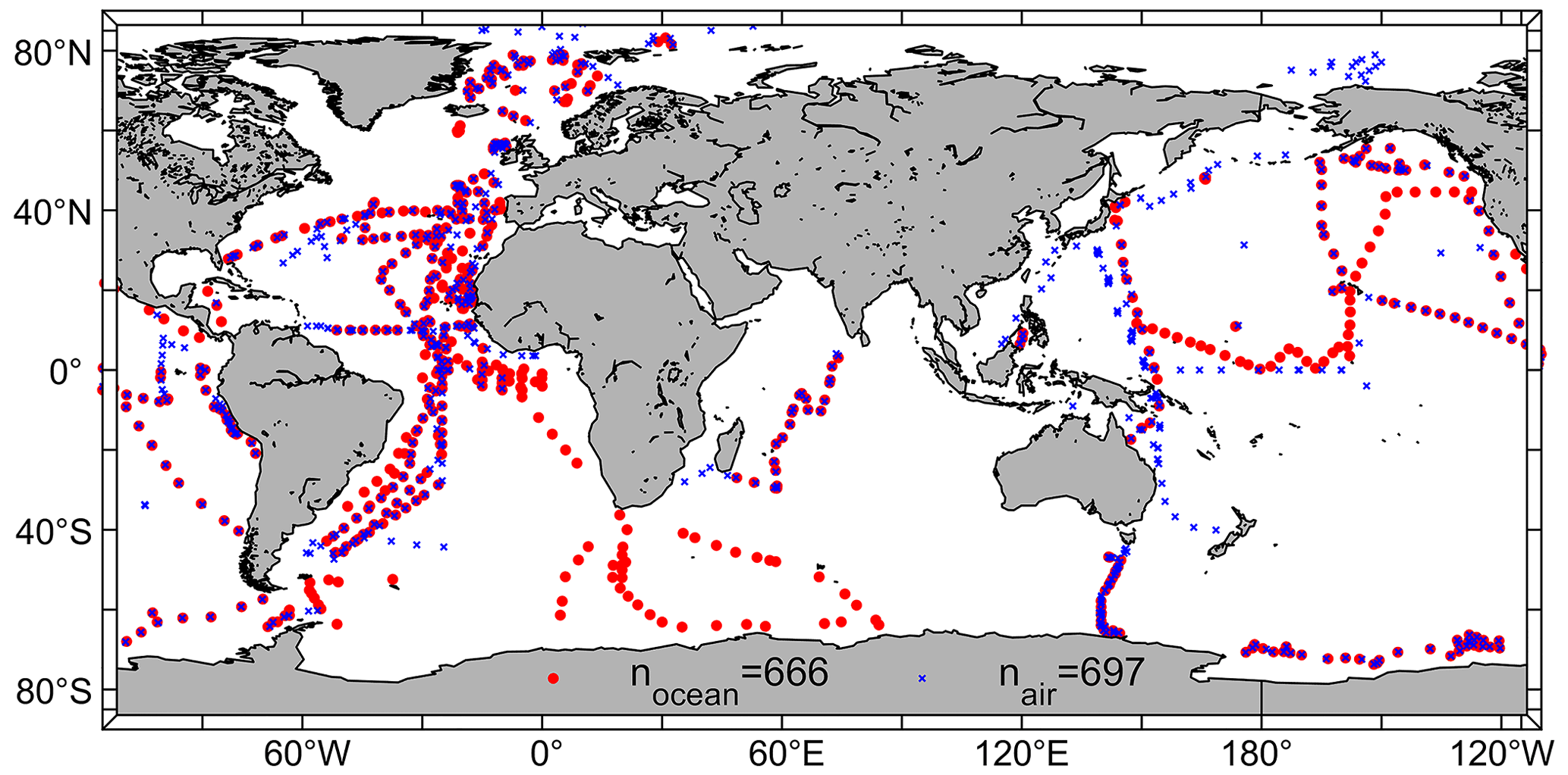
Figure 1 Locations of daily mean oceanic CHBr₃ observations (shown as red dots (n=666)) and atmospheric CHBr₃ observations (shown as blue dots (n=697)) from the HalOcAt database for comparison with the daily mean NorESM2 model output.

2.4 Bromoform excess/deficit calculation

The CHBr₃ excess/deficit (balance) rate (k_bal in Eq. (15) (pmol m⁻² h⁻¹)) is the difference between the CHBr₃ production rate and the sum of different CHBr₃ loss rates, with all rates integrated over the upper 100 m depth. It is given as

$$\begin{array}{}\text{(15)}& \begin{array}{rl}{k}_{\mathrm{bal}}& =\sum \mathrm{production}\mathrm{rate}-\sum \mathrm{loss}\mathrm{rate}=k_{\mathit{\beta }}\\ & -\left(k_{\mathrm{UV}}+k_{\mathrm{F}}\right).\end{array}\end{array}$$

The production term is described as the biological oceanic CHBr₃ production rate, k_β (Eq. 2), and the loss term includes the two fastest loss processes – i.e., photolysis due to UV radiation, k_UV (Eq. 7), and the loss to the atmosphere via air–sea gas exchange, k_F (Eq. 3). We define a positive k_bal as the CHBr₃ excess rate and a negative k_bal as the CHBr₃ deficit rate. The loss terms related to hydrolysis and to halogen substitution are not included as they are several orders of magnitude smaller than k_UV and k_F in the surface ocean.

2.5 Calculation of drivers for oceanic CHBr₃ and atmospheric CHBr₃ and their emissions

Different parameters impact the variations in oceanic and atmospheric CHBr₃ values and influence the air–sea gas exchange. These impacts can vary in magnitude and frequency depending on local and seasonal conditions. Daily mean model output values from 1990–2014 were used to calculate annually and seasonally resolved – December–January–February (DJF), March–April–May (MAM), June–July–August (JJA), and September–October–November (SON) – driving factors for oceanic CHBr₃ concentrations (Bromo_oce), atmospheric CHBr₃ mixing ratios (Bromo_air), and CHBr₃ fluxes (Bromo_flux) in three specific areas (North Atlantic, tropical West Pacific, Southern Ocean); these are presented in Sect. 3.4. Driving factors for each area, parameter, and season were derived using multilinear regression (MLR) analyses.

In order to compare parameters with different magnitudes, input data of each parameter were standardized prior to the MLR analysis by centering them to have a mean of 0 and scaling them to have a standard deviation of 1. Input data for each parameter consisted of daily averages over the specific area, providing 365 values as a basis for annually resolved MLR and ∼ 90 values for seasonally resolved MLR.

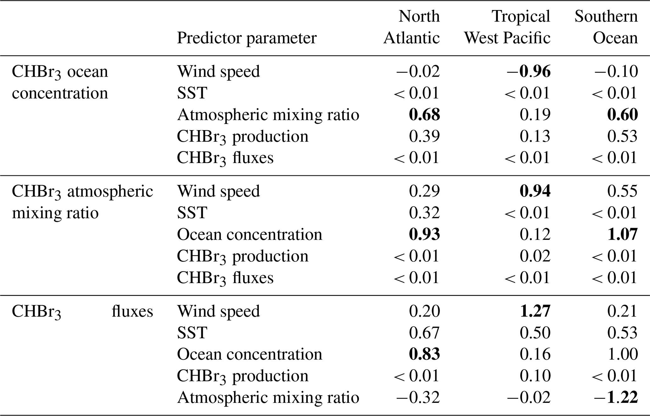
A schematic summarizing the relationships between the different parameters in Eqs. (S1)–(S3) is shown in Fig. 2, including CHBr₃ production (Bromo_prod); 10 m surface wind speed (wind); sea surface temperature (SST); and the derived parameters Bromo_oce, Bromo_air, and Bromo_flux. Other oceanic CHBr₃ loss processes (e.g., photolysis) were neglected in these calculations as the loss due to gas exchange is approximately 70 times higher than the loss due to photolysis (data not shown). If the highest resulting coefficient for each season and MLR is significantly higher than all other coefficients, the corresponding parameter is presented as the main driver for Bromo_oce, Bromo_air, or Bromo_flux. If the highest resulting coefficient is not significantly different from the second- or third-highest coefficient, more than one coefficient and corresponding parameters are presented as main drivers. Table 1 lists the annual mean coefficients, and Table S1 lists the seasonally resolved main drivers.

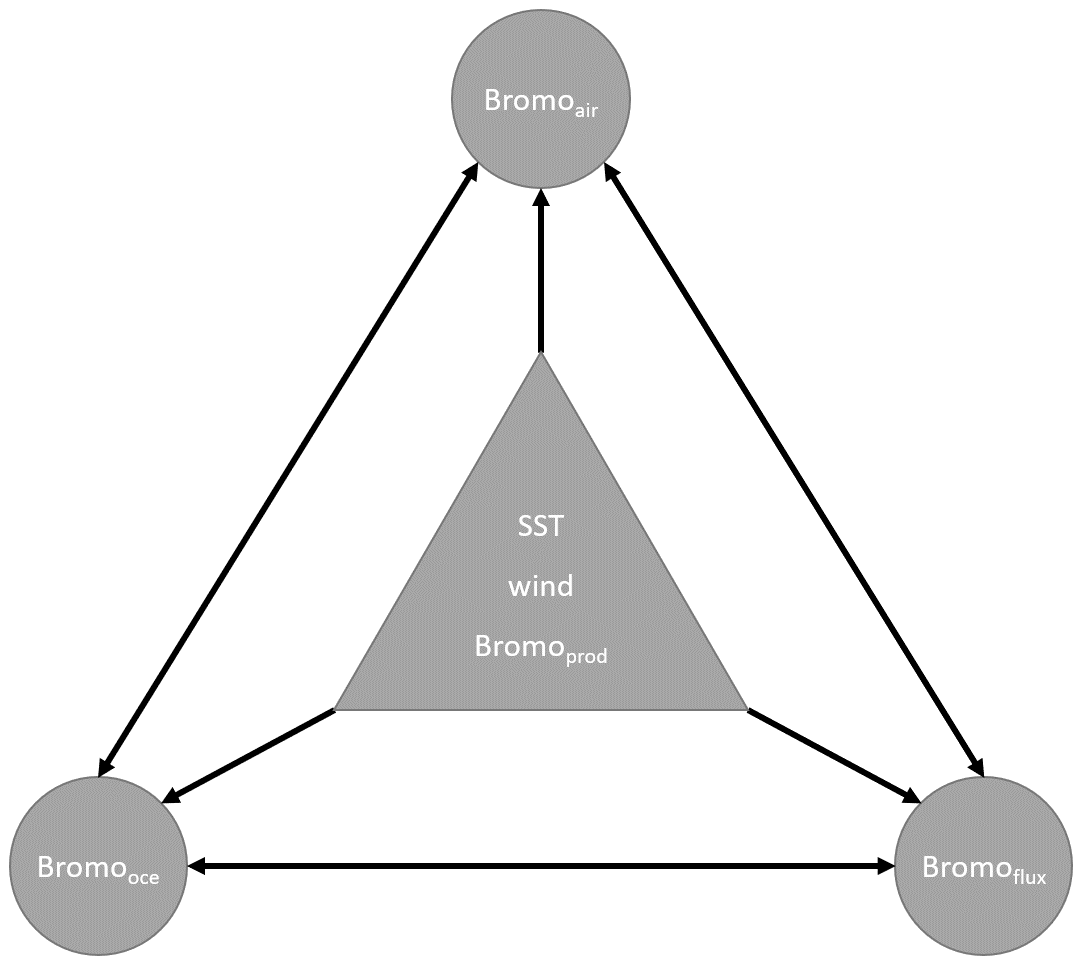
Figure 2 Schematic illustration of relationships between different parameters influencing each other. Generic parameters (in the triangle) influence the derived parameters (in the circles). Each derived parameter in a circle is influenced by all five other parameters. The relationships form the basis for the multilinear regression analysis using Eqs. (S1)–(S3).

3 Results and discussion

3.1 Model climatology

The annual and seasonal oceanic CHBr₃ concentrations, atmospheric mixing ratios, and emissions reveal significant spatial variations (Figs. 3 and S1). The annual global average of surface CHBr₃ concentrations is 5.04 pmol L⁻¹ (DJF: 5.36 pmol L⁻¹; JJA: 4.86 pmol L⁻¹), with the highest annual mean concentrations of 28.37 pmol L⁻¹ in the upwelling region off the coast of Peru and the lowest annual mean concentrations of 1.37 pmol L⁻¹ in the Gulf of Boothia (71° N, 91° W), north of Canada. The areas with the lowest oceanic CHBr₃ concentrations are the central parts of the North and the South Pacific gyres. Concentrations of surface ocean CHBr₃ in the entire NH (JJA (5.9 pmol L⁻¹) > DJF (4.3 pmol L⁻¹)) and SH (DJF (6.1 pmol L⁻¹) > JJA (4.1 pmol L⁻¹)) are generally higher during the respective summer than during the respective winter. These distinct differences in oceanic CHBr₃ concentrations are also due to higher biological production in summer (NH: 335 pmol m⁻² h⁻¹; SH: 371 pmol m⁻² h⁻¹) than in winter (NH: 235 pmol m⁻² h⁻¹; SH: 173 pmol m⁻² h⁻¹), as shown in Fig. S3 and discussed in Sect. 3.4. The direct link of CHBr₃ to biological production applies to the low oceanic CHBr₃ concentrations in the North and South Pacific gyres and to the high oceanic concentrations in the areas of the EBUSs.

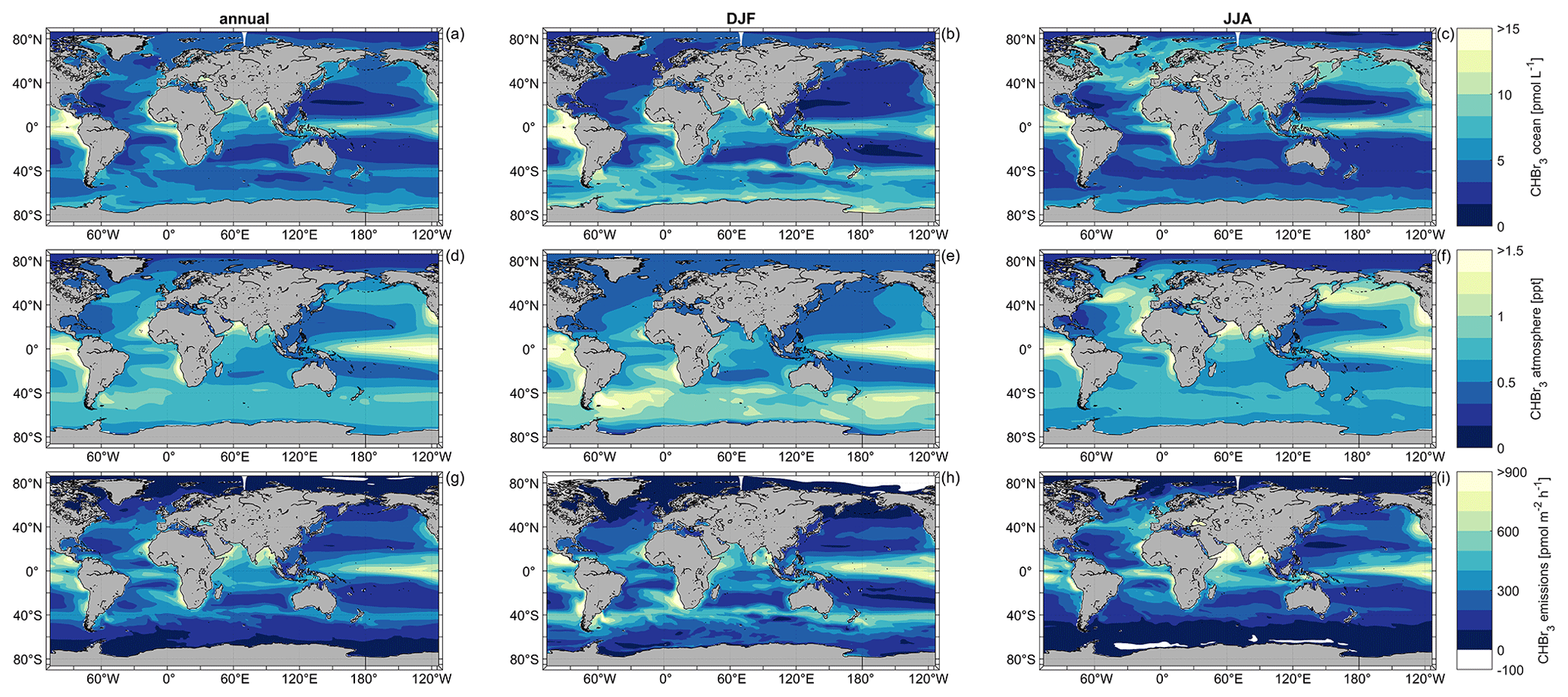
Figure 3 Simulated annual (a, d, g), DJF (b, e, h), and JJA (c, f, i) mean oceanic surface CHBr₃ concentrations (a, b, c), atmospheric mixing ratios (d, e, f), and CHBr₃ emissions (g, h, i) for the period 1990–2014.

Variations in annual mean atmospheric CHBr₃ mixing ratios mainly follow the surface ocean concentrations, with the highest mixing ratios in the tropics, especially in the EBUSs. Global annual average mixing ratios over the ocean stand at 0.67 ppt (DJF: 0.70 ppt; JJA: 0.69 ppt), with the highest annual mean mixing ratios reaching 2.21 ppt in the southeastern Pacific upwelling region off the coast of Peru and the lowest annual mean mixing ratios reaching 0.13 ppt over the Persian Gulf. On a global average, the variability in atmospheric mixing ratios is lower than the variability in CHBr₃ concentrations in the surface ocean (Figs. 3 and S2). During austral winter (JJA), mostly dark and cold conditions increase the lifetime of atmospheric CHBr₃, which leads to a uniform mixing ratio (0.67 ± 0.05 ppt) over the entire Southern Ocean. Similar to oceanic CHBr₃ concentrations, central parts of the North and South Pacific gyres have low atmospheric CHBr₃ mixing ratios (0.46 ± 0.05 ppt). During austral summer (DJF), atmospheric mixing ratios increase further as strong biological activity increases surface ocean concentrations, which enhance the oceanic emissions. Further seasonal-dependent driving factors for specific regions are discussed in Sect. 3.4.

Generally, supersaturation of CHBr₃ in the world's ocean leads to emissions from the ocean to the atmosphere (defined as positive fluxes). Global annual mean fluxes are 268 pmol m⁻² h⁻¹ (DJF: 294 pmol m⁻² h⁻¹; JJA: 253 pmol m⁻² h⁻¹), with the highest annual mean fluxes of 953 pmol m⁻² h⁻¹ in the upwelling region off the coast of Peru. In the tropical regions, annual mean fluxes of 427 pmol m⁻² h⁻¹ between 10° N and 10° S contribute to the atmospheric entrainment of oceanic CHBr₃ into the stratosphere (Fiehn et al., 2018; Tegtmeier et al., 2020). The lowest annual mean fluxes of −1 pmol m⁻² h⁻¹ are modeled under ice-free conditions in the Gulf of Boothia (71° N, 91° W), north of Canada (white regions in Fig. 3), with very low oceanic CHBr₃ production and low seawater temperatures. However, the atmospheric mixing ratios are comparably high under these conditions. These conditions favor negative fluxes, which, according to the results of our fully coupled ESM, can be seen in the Arctic and Antarctic during winter, confirming the results by Stemmler et al. (2015) and Ziska et al. (2013), although with a lower magnitude.

Generally, the modeled CHBr₃ emissions are high where the ocean concentration is high, and the elevated emissions lead to elevated atmospheric mixing ratios. However, due to oceanic transport processes, locations of high oceanic CHBr₃ emissions do not always coincide with locations of high oceanic CHBr₃ production (compare Figs. 3 and S3). In the northern part of the Bay of Bengal (> 18° N), for example, ocean concentrations during DJF are very high (on average, 21.64 pmol L⁻¹), while emissions are not as high compared to other ocean regions due to low wind speeds. This leads to a lower atmospheric mixing ratio than expected from the oceanic concentrations and shows that oceanic CHBr₃ concentrations, emissions, and atmospheric mixing ratios show regionally different interdependencies, which is addressed in detail in Sect. 3.4.

3.2 Model validation with observations

The annual mean of the surface oceanic CHBr₃ concentration (Fig. 4a) from the 666 daily mean observations is ${\mathrm{5.02}}_{\mathrm{0.05}}^{\mathrm{28.21}}$ (${\mathrm{mean}}_{\min }^{\max })$ pmol L⁻¹. The global annual mean of the surface oceanic CHBr₃ concentration from the model using only locations corresponding with existing observations is ${\mathrm{6.61}}_{\mathrm{1.39}}^{\mathrm{24.25}}$ pmol L⁻¹. These results indicate that the model values are within the range of observed concentrations of oceanic CHBr₃. While the mean concentration of the model is higher than the mean of the observations, all validated model data points fall within the full range of the observations. The model data cover a grid of ∼ 100 km resolution, which leads to a smoothing of the values, whereas observational data are local daily mean point data.

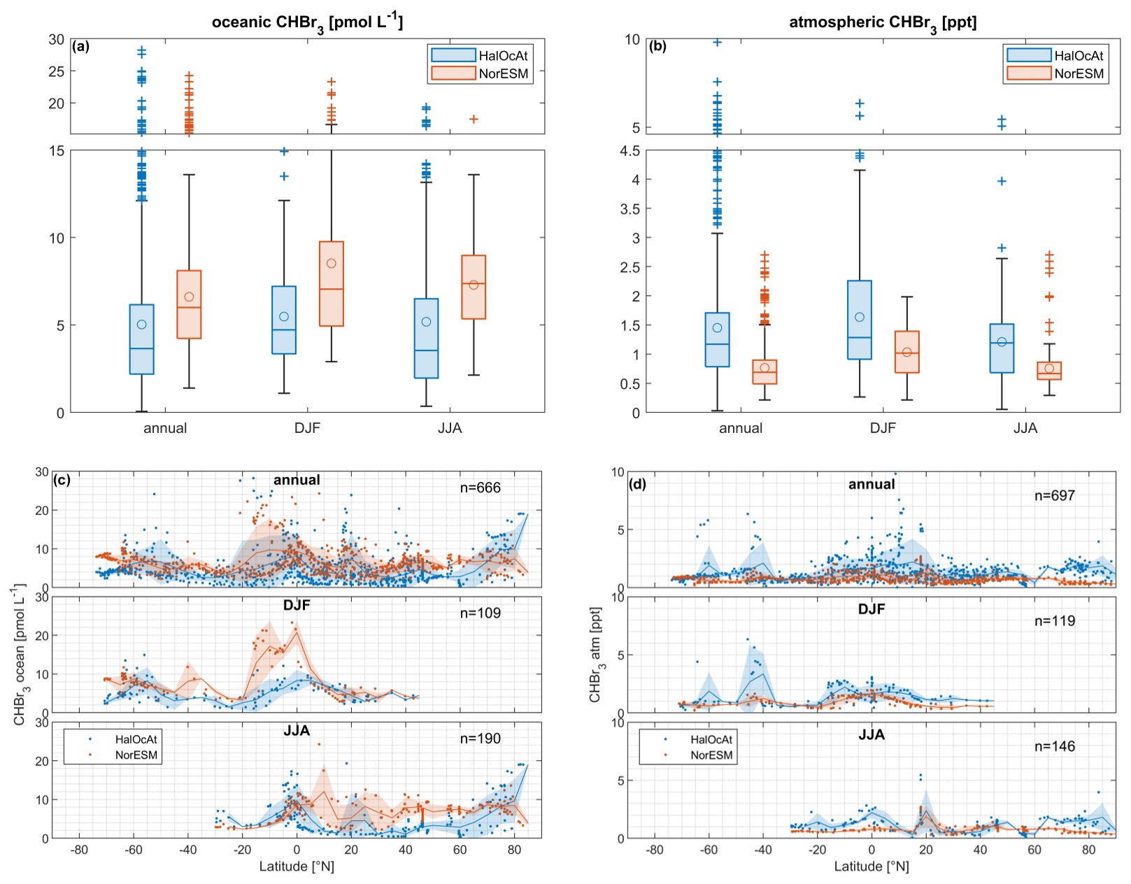
Figure 4 Boxplot comparison of NorESM2 model results with HalOcAt observations for oceanic (a) and atmospheric (b) CHBr₃. (c) Comparison of zonal-mean oceanic CHBr₃ on an annual scale and in DJF and JJA. (d) Comparison of zonal-mean atmospheric CHBr₃ on an annual scale and in DJF and JJA. Shaded areas represent standard deviations from 5° zonal bin averages. Boxplots (a, b) have a break in the y axis to increase readability of the figure. The horizontal line inside the box represents the median value. The circle shows the mean value. The boxes show the first to third quartiles, and the whiskers illustrate the highest and lowest values that are not outliers. The plus signs represent outliers. Note that “atm” stands for atmosphere.

The mean CHBr₃ atmospheric mixing ratio (Fig. 4b) from the 697 daily mean observations is ${\mathrm{1.45}}_{\mathrm{0.03}}^{\mathrm{9.80}}$ ppt. The global mean atmospheric mixing ratio of CHBr₃ from the model at locations with observations is ${\mathrm{0.76}}_{\mathrm{0.22}}^{\mathrm{2.70}}$ ppt. This comparison shows that the observed atmospheric mixing ratios of CHBr₃ are of the same magnitude but generally higher than those from the model output. While our model experiment focuses on natural CHBr₃ production by means of phytoplankton, other sources, such as coastal macroalgae (Carpenter and Liss, 2000) and anthropogenic sources, e.g., power plant cooling (Maas et al., 2021) or desalination plants (Agus et al., 2009), may explain parts of the higher global annual median of the observational data, which comes to 41 %. Jia et al. (2023) calculated an increase in global CHBr₃ emissions of 31.5 % when including anthropogenic emissions, which may also partly explain the lower atmospheric mixing ratios in the model compared to the observations.

Figure 4 also shows a more detailed comparison between observations and model data in 5° zonally binned averages (shaded areas) for oceanic (Fig. 4c) and atmospheric (Fig. 4d) CHBr₃ on an annual basis as well as in JJA and DJF. The modeled data compare well with observations of oceanic CHBr₃ (Fig. 4c) on annual basis across the 5° latitudinal bins. In the HalOcAt database, there are no oceanic and atmospheric observations available north of 50° N and south of 30° S during boreal winter (DJF) and austral winter (JJA), respectively, which highlights the need for model data to entirely describe spatially and temporally resolved CHBr₃ (see also Fiehn et al., 2018). During DJF, the model overestimates the measured concentrations between 20° N and 5° S. During JJA, averaged model concentrations in the NH (10–60° N) are slightly higher than in the averaged observations. These discrepancies could indicate a missing process understanding, revealing lower oceanic production or additional loss processes.

With all data available, the 5° latitudinal-averaged atmospheric CHBr₃ observations show a large spread in the tropics, resulting in a high standard deviation (Fig. 4d). The model results in this region are uniform with a much lower standard deviation. During boreal winter (DJF), atmospheric CHBr₃ observations and model results show good agreement, with an exception at 40–50° S. In this latitude range, observational atmospheric CHBr₃ mixing ratios (> 3 ppt; Fig. 4d) were recorded between 24 and 60° W in the South Atlantic in 2007 (Gebhardt, 2008). Gebhardt (2008) reports enhanced biological production in the Argentinian shelf-break zone (55–60° W), with an elevated chlorophyll-a concentration of up to 4.5 µg L⁻¹. These values also suggest a high production of CHBr₃ and subsequent high emissions to the atmosphere. The prevailing westerly winds transported the CHBr₃-enriched air masses eastward to the remote South Atlantic region in 2007, while in the model, lower biological production entails lower atmospheric mixing ratios compared to the observations. During boreal summer (JJA), very good agreement between atmospheric observations and model results is obtained between 10 and 60° N. North of 60° N, the model underestimates the measured atmospheric mixing ratios in the polar region. Local meteorological and biological conditions (e.g., high wind speed and distinct phytoplankton blooms) are averaged by the model to a resolution of ∼ 100 km. Averaging data over time or space leads to lower mean values, i.e., gas emissions (Bates and Merlivat, 2001), in the model. This explains the lower modeled atmospheric mixing ratios compared to the observations on a global scale and anthropogenic CHBr₃ sources (Jia et al., 2023). Furthermore, discrepancies between model results and observations also point to a lack of process understanding, which helps to improve our understanding of the biogeochemical cycling of CHBr₃. For our CHBr₃ production rate, we used the highest production rate, which we could retrieve from the published data (Roy, 2010; Kurihara et al., 2012). Therefore, we likely have not underestimated the oceanic planktonic source in general, and either the production rates are too high or the sink rates are too low in some regions (e.g., the equatorial Pacific). Furthermore, the resulting model bias does not follow a spatial pattern (Fig. S4). We claim that currently not enough observational or experimental information is available to pinpoint the answer. As pointed out, the underestimation of atmospheric CHBr₃, despite the maximum of the planktonic CHBr₃ source, is likely due to averaging, a missing source for the atmosphere, or even the parameterization of marine CHBr₃ fluxes yielding emissions with values that are too low. Despite the named uncertainties, which deserve further studies, the model reflects the data very well and thereby the current status of knowledge.

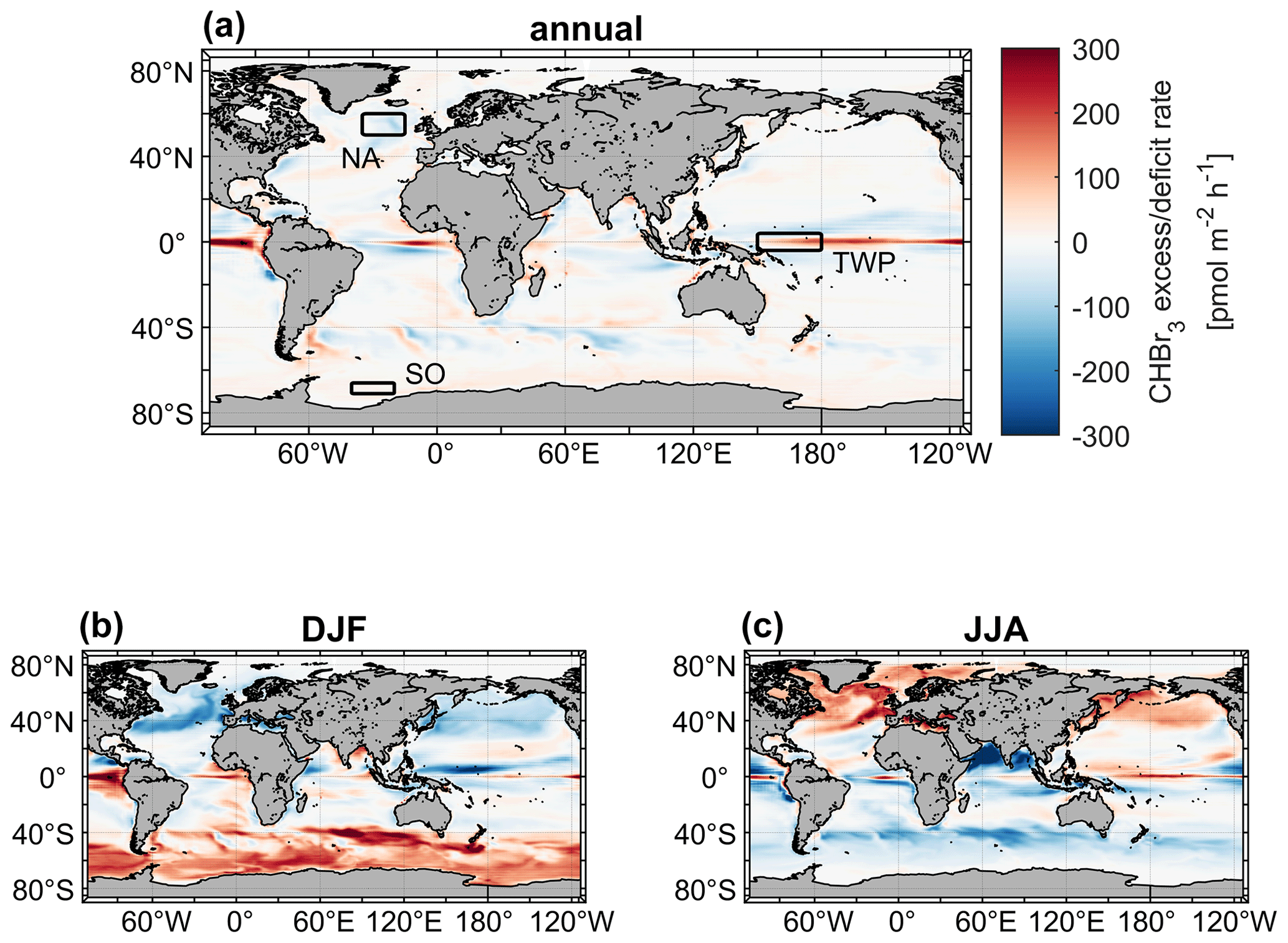
Figure 5 Mean CHBr₃ excess/deficit rates on an annual (a) and seasonal (DJF: b; JJA: c) basis. The three rectangles in (a) illustrate the locations of the case studies. NA: North Atlantic. TWP: tropical West Pacific. SO: Southern Ocean.

3.3 Excess and deficit regions of oceanic bromoform

In most of the world's surface oceans (e.g., the North and South Pacific oceans) CHBr₃ production and loss rates are balanced on an annual average with k_bal close to zero (Fig. 5a). The Equator region experiences a strong excess rate (positive k_bal) on an annual average with values of up to 300 pmol m⁻² h⁻¹, indicating higher CHBr₃ production than loss in the upper ocean, caused by strong primary production (Fig. S3) in the equatorial upwelling. Surface currents transport CHBr₃-enriched surface water masses away from the Equator while experiencing loss of CHBr₃ to the atmosphere. Therefore, adjacent marine areas north and south of the Equator experience a deficit rate (negative k_bal) of CHBr₃ (blue areas in Fig. 5) as no production balances the loss. The seasonality of k_bal is pronounced in the extratropics (Fig. 5b and c). In these regions, a CHBr₃ excess rate is observed mainly during summer and a CHBr₃ deficit rate mainly during winter in the respective hemispheres. A high k_β (elevated biological production) and a low k_F (weak emissions to the atmosphere), caused by lower winds during summer, lead to a higher CHBr₃ surface ocean concentration in summer than in winter (Fig. 3). During winter in both hemispheres, lower biological activity (low k_β) and elevated wind speed (high k_F) decrease CHBr₃ production and increase emissions to the atmosphere, which leads to a CHBr₃ deficit rate. These results reveal seasonal and spatial differences in parameters (driving factors), which influence CHBr₃ concentrations in the world's ocean.

In the following subsection, we select three different case study areas, indicated in Fig. 5, in order to contrast the driving factors of the variations in oceanic and atmospheric CHBr₃ on regional and temporal scales. These case studies are as follows:

• the North Atlantic, with an annual mean CHBr₃ deficit rate ($k_{\mathrm{bal}}=-\mathrm{33}$ pmol m⁻² h⁻¹);

• the tropical West Pacific, with an annual mean CHBr₃ excess rate ($k_{\mathrm{bal}}=+\mathrm{32}$ pmol m⁻² h⁻¹);

• the Southern Ocean, with negative fluxes during the respective winter ($k_{\mathrm{bal}}=+\mathrm{15}$ pmol m⁻² h⁻¹).

3.4 Driving factors of bromoform on regional and temporal scales

This section investigates the seasonal changes in oceanic and atmospheric CHBr₃ and other parameters in three contrasting regions. Daily means of oceanic CHBr₃ concentrations, production, fluxes, balance (as defined in Eq. 15), and atmospheric mixing ratios; SST; and wind speed over an entire year reveal large differences between the North Atlantic, tropical West Pacific, and Southern Ocean (Fig. 6). Using MLR analysis, the main driving factors of variability in oceanic CHBr₃, atmospheric CHBr₃, and their fluxes in each region and season are investigated.

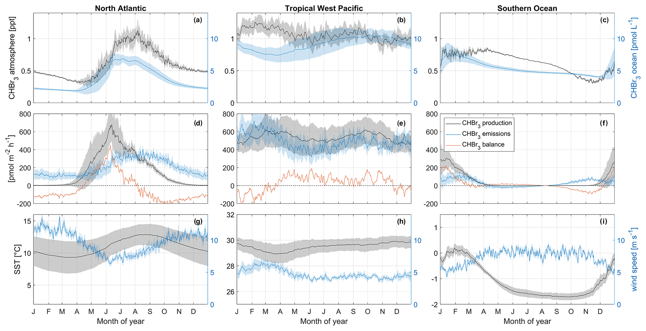
Figure 6 Seasonal changes in oceanic and atmospheric CHBr₃ (a–c); CHBr₃ production, emissions, and balance (d–f); and SST and wind speed (g–i). These changes are shown for the North Atlantic (a, d, g), tropical West Pacific (b, e, h), and Southern Ocean (c, f, i). Shaded areas each represent 1 standard deviation of the average value in the corresponding area. Note that y limits for SST are not similar between the three regions in order to increase the readability of the figure.

3.4.1 North Atlantic

The North Atlantic region (50–60° N, 15–35° W) is characterized by a strong seasonal cycle of both oceanic CHBr₃ concentrations and atmospheric mixing ratios (Fig. 6a). The magnitude of the cycle is the strongest among the three investigated regions (compare with Fig. 6b and c). Oceanic CHBr₃ concentrations are on average 3.64 pmol L⁻¹ (min: 1.87 pmol L⁻¹ at the end of March; max: 6.93 pmol L⁻¹ during July). Atmospheric mixing ratios show a similar seasonal cycle, shifted by 1 month, with average values of 0.60 ppt, a minimum mixing ratio of 0.30 ppt during April, and a maximum mixing ratio of 1.12 ppt during August. The CHBr₃ emissions (199 ± 91 pmol m⁻² h⁻¹) follow the patterns of both oceanic and atmospheric values (Fig. 6d). The seasonal cycle of CHBr₃ production (171 ± 191 pmol m⁻² h⁻¹) is similar to the cycle of CHBr₃ concentration, while the sharp peak in May and June when the spring phytoplankton bloom evolves in the North Atlantic is not reflected in the oceanic concentrations. The strong production leads to a CHBr₃ excess rate during summer (JJA: 103 pmol m⁻² h⁻¹) and a CHBr₃ deficit rate in winter (DJF: −114 pmol m⁻² h⁻¹) (Fig. 6d).

The MLR analysis indicates that on an annual basis, variations in atmospheric mixing ratios are mainly associated with CHBr3 ocean concentrations (Table 1) and vice versa (Fig. 7a and d). A higher surface water CHBr3 concentration increases the emissions to the atmosphere, resulting in increasing atmospheric mixing ratios. According to the MLR analysis, on a seasonal basis, oceanic CHBr3 concentrations are mainly driven by the oceanic production during MAM and SON (Table S1), which increases sharply from March to June to 680 pmol m⁻² h⁻¹ before gradually decreasing in SON (Fig. 6d). Atmospheric mixing ratios are mainly driven by oceanic concentrations (Fig. 7d; Table 1; R²=0.89, p value < 0.05). Only in winter (DJF), when hardly any production occurs, do low SSTs, which increase the solubility of CHBr₃, drive the variations in atmospheric mixing ratios (Table S1; R²=0.95, p value < 0.05). Thus, the emissions decrease, even during high wind speeds, which leads to lower atmospheric CHBr₃. The emissions are mainly driven by the oceanic concentrations (Fig. 7g; Table 1; R²=0.81, p value < 0.05) over the course of a year, while during spring (MAM), wind speed, SST, and CHBr₃ production drive the emissions equally (Table S1). While CHBr₃ production and SSTs increase, surface wind speed decreases, and emissions are pretty constant at 130 ± 29 pmol m⁻² h⁻¹ (Fig. 6d). During summer (JJA), low winds and a high oceanic CHBr₃ concentration equally increase the emissions (Table S1). In contrast to during spring, higher SSTs (lower solubility) are only of minor importance during JJA, while in fall and winter, decreasing SSTs are the main drivers again, along with high atmospheric mixing ratios, which additionally dampen the emissions (Table S1).

3.4.2 Tropical West Pacific

Figure 5 shows that the equatorial regions of the Atlantic and Pacific oceans are sources of oceanic CHBr₃, which is transported to other oceanic regions by ocean currents. Oceanic CHBr₃ concentrations in the tropical West Pacific (4° S–4° N, 150°–180° E) show a reduced seasonal cycle compared to the above-discussed North Atlantic region (Fig. 6b), while the average of 9.11 pmol L⁻¹ is significantly higher than in the North Atlantic. Also, CHBr₃ production (536 ± 42 pmol m⁻² h⁻¹), CHBr₃ fluxes (492 ± 84 pmol m⁻² h⁻¹), and atmospheric mixing ratios (1.07 ± 0.08 ppt) show hardly any seasonality (Fig. 6b and e). The same is true for SST (29.50 ± 0.28 °C) and wind speed (4.71 ± 0.76 m s⁻¹) (Fig. 6h). The CHBr₃ balance is positive throughout the whole year except during DJF (Fig. 6e). During this period, higher wind speed entails higher emissions. Production rates are lower and induce a CHBr₃ deficit. However, this deficit does not compensate for the CHBr₃ excess during the rest of the year, leading to an overall excess of 32 pmol m⁻² h⁻¹.

MLR analysis shows that wind speed is the main factor influencing the variations in oceanic CHBr₃ concentrations, CHBr₃ atmospheric mixing ratios, and CHBr₃ fluxes on an annual basis (Fig. 7b, e, and h; Table 1). During JJA and SON, CHBr₃ production drives CHBr₃ concentrations (Table S1), which increase from 477 pmol m⁻² h⁻¹ in July to 618 pmol m⁻² h⁻¹ by the end of September. This results in an increase in oceanic CHBr₃ concentrations as all other parameters stay constant during that period.

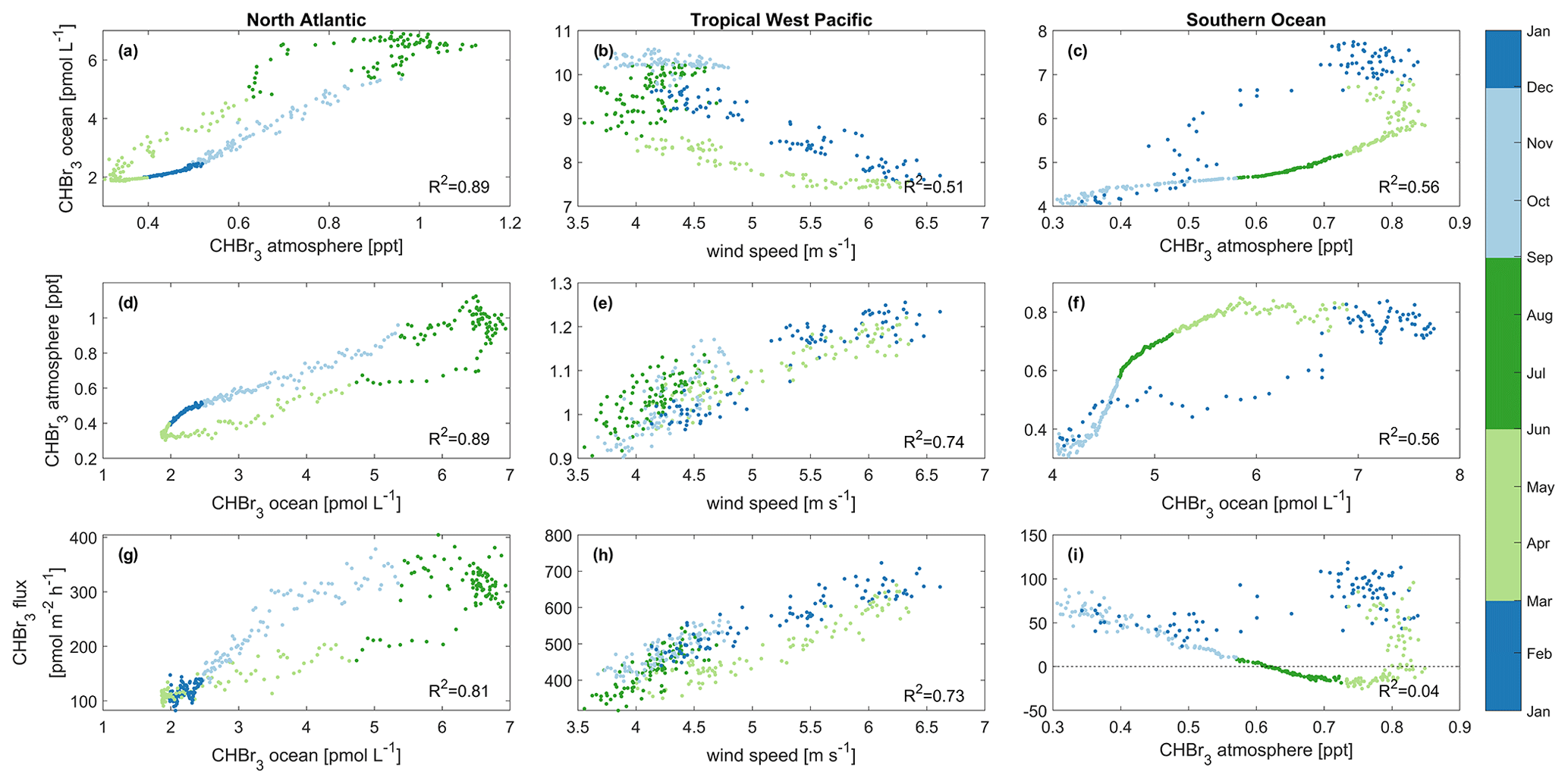
Figure 7 Main drivers of oceanic CHBr₃ concentrations (a, b, c), atmospheric mixing ratios (d, e, f), and CHBr₃ emissions (g, h, i). These drivers are shown for the North Atlantic (a, d, g), tropical West Pacific (b, e, h), and Southern Ocean (c, f, i). Different colors denote different seasons of the year. Each data point represents a daily average over the specific case study area. Statistical analysis for each of the nine datasets indicates significant correlation (p value < 0.05) with the coefficient of determination (R²) listed in the bottom right of each panel. Please be aware that panels (a) and (d) as well as (c) and (f) contain the same information only with interchanged x and y axes as both parameters, oceanic and atmospheric bromoform, are interdependent in the two regions.

3.4.3 Southern Ocean

The selected Southern Ocean region (71–66° S, 40–20° W) experiences generally negative water temperatures (mean: −1.08 °C) throughout the year (Fig. 6i). The minimum of −1.71 °C is reached in September, and the maximum of +0.19 °C is reached in January/February. Wind speed is nearly constant throughout the year (7.33 m s⁻¹), decreasing only during austral summer (DJF; Fig. 6h) to 5.76 m s⁻¹. Oceanic CHBr₃ concentrations are on average higher (5.38 pmol L⁻¹) than in the North Atlantic region. Maximum concentrations of 7.74 pmol L⁻¹ are reached in January, and the lowest concentrations of 4.04 pmol L⁻¹ are reached at the end of December. Due to low SSTs and a short day length, CHBr₃ production rates are almost zero from May to October and increase to 306 pmol m⁻² h⁻¹ in January (Fig. 6f). Atmospheric mixing ratios are highest (0.85 ppt) from January to the beginning of April and decline very slowly (Fig. 6c) under the following low light levels until they reach their minimum of 0.31 ppt in November. Constantly high atmospheric mixing ratios, very low SSTs, and decreasing oceanic CHBr₃ concentrations after the short summer bloom in DJF influence the switch from emissions to negative fluxes between April and July (Fig. 6f). CHBr₃ is in excess during times of production (DJF), is almost balanced during fall and winter from April to September (Fig. 6f), and shows a slight excess of 15 pmol m⁻² h⁻¹ annually.

Atmospheric mixing ratios are the main factor influencing the variations in oceanic concentrations (Fig. 7c; Table 1; R²=0.56, p value < 0.05), while during fall (MAM; Table S1), CHBr₃ production is their driving factor. During this time, CHBr₃ production decreases and so do the ocean concentrations (Fig. 6c and f). Atmospheric mixing ratios are mainly driven by high oceanic CHBr₃ concentrations in DJF (R²=0.88, p value < 0.05) and by SST during cold JJA (R²=0.95, p value < 0.05) (Table S1). Low light levels increase the lifetime of atmospheric CHBr₃ in JJA, and low SSTs increase the solubility of oceanic CHBr₃, both leading to decreased emissions during winter (JJA). CHBr₃ emissions are mainly driven by SST in summer (DJF) (Table S1; R²=0.60, p value < 0.05) as the solubility of CHBr₃ in the ocean decreases due to increasing SSTs. After this short summer period, temperatures decline in fall (MAM) and increase the solubility of oceanic CHBr₃, which results in decreased emissions (Fig. 6f and i). During winter (JJA) and spring (SON), SSTs and oceanic CHBr₃ concentrations stay low, and therefore, increasing emissions are mainly driven by decreasing atmospheric mixing ratios.

In summary, the three different regions clearly indicate that driving factors for atmospheric and oceanic bromoform, as well as for bromoform fluxes, are dependent on local conditions. Planktonic production, which is the only source of CHBr₃ in the model setup, impacts the variability in oceanic CHBr₃ concentrations only in regions with a distinct seasonality in biological production (i.e., North Atlantic, Southern Ocean). During times of lower productivity, atmospheric mixing ratios influence oceanic CHBr₃ concentrations. In subpolar and polar regions (i.e., Southern Ocean), oceanic CHBr₃ and its subsequent fluxes are driven by the solubility of CHBr₃, which is related to low SST in late winter and spring (i.e., sea ice melt). Although wind speed is an important parameter for air–sea gas flux, this study reveals that wind speed is only the main driver for oceanic and atmospheric CHBr₃ variability in areas with low seasonality (i.e., the tropical West Pacific).

These results demonstrate the benefits of simulating CHBr₃ in a fully coupled ESM configuration to calculate driving factors for different parameters on a temporal and spatial basis. Studying the influence of one or more parameters on the variability in other parameters in the model is not realistic when using prescribed oceanic concentrations or atmospheric mixing ratios. Investigating CHBr₃ cycling in different locations and on different timescales helps us to understand the interconnections and to better integrate their results into both current and future climate models.

Table 1 Annual coefficients of predictors for each MLR in the different case studies. Bold coefficients indicate the highest values within an MLR analysis of one parameter and region and act as an indicator for the driving factors of the predicted parameter (Eqs. S1–S3).

3.5 Global bromoform emission inventories

A comparison of our modeled versus published global CHBr₃ emissions is presented in Fig. 8. Global annual CHBr₃ emissions from top-down approaches are 449, 528, and 592 Gg yr⁻¹ based on calculations from Liang et al. (2010), Ordóñez et al. (2012), and Warwick et al. (2006), respectively. These inventories are about 2 to 8 times higher than calculated annual emissions from bottom-up approaches, which range from 76 Gg yr⁻¹ (Stemmler et al., 2015) to 238 Gg yr⁻¹ (Lennartz et al., 2015). Our results (214 Gg yr⁻¹) are similar to the emission estimates of 215 Gg yr⁻¹ published by Ziska et al. (2013) but are significantly higher than the estimate of 76 Gg yr⁻¹ given by Stemmler et al. (2015), which is based on oceanic CHBr₃ observations from the HalOcAt database.

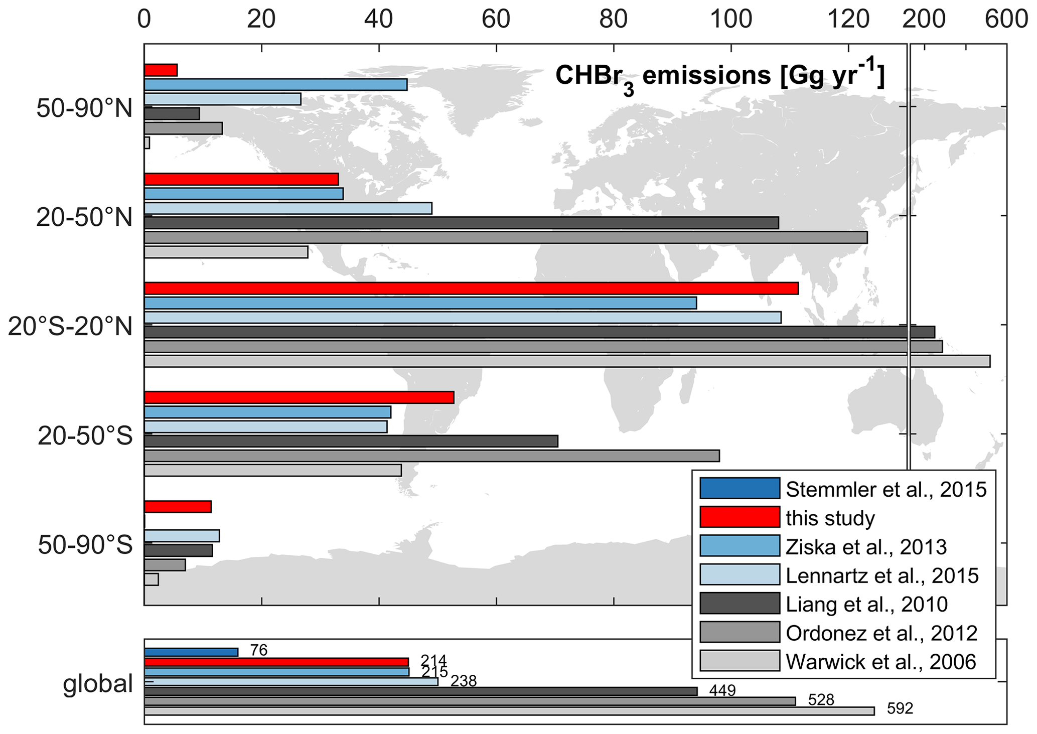
Figure 8 Comparison of global and latitudinally binned annual CHBr₃ emissions from different studies. The grey and blue bars denote top-down approaches and bottom-up approaches, respectively.

As we apply a CHBr₃ production rate in the ocean that is 2.38 times higher than that of Stemmler et al. (2015), we simulate a production rate of 0.88 Gmol yr⁻¹ compared to their 0.37 Gmol yr⁻¹. Our emissions (214 Gg yr⁻¹) are 2.82 times higher (global values in Fig. 8) than the emission estimate (76 Gg yr⁻¹) given by Stemmler et al. (2015). Our model adaption is based on a higher bulk CHBr₃ production ratio (β₀), based on Kurihara et al. (2012) and Roy (2010) (see Sect. 2.1.1). This production rate is at the higher end of the published values. Therefore, the resulting CHBr₃ production can be seen as an upper limit. Moreover, the ratio of bromoform emissions (2.82) is higher than the ratio of bromoform production (2.38) and indicates an excess of 18 %. This is caused by the prescribed mean atmospheric values, without any seasonality, used in Stemmler et al. (2015) and becomes more significant at higher latitudes, where the seasonality of bromoform emissions becomes more important (Fiehn et al., 2018). Especially during winter, the annually prescribed mean atmospheric values are too high and artificially dampen bromoform emissions. This results in a higher emission estimate using our fully coupled model approach.

Comparing bottom-up and top-down approaches, the annual CHBr₃ emissions from the tropics (20° S–20° N in Fig. 8) account for ∼ 47 % (105 Gg yr⁻¹) and ∼ 66 % (351 Gg yr⁻¹) of global emissions, respectively. However, the tropics only account for ∼ 37 % of the global oceanic surface area, underlining this region as the most important source region of CHBr₃ on Earth.

Emissions in the middle latitudes (20 to 50° N/S) of the NH and SH show a similar distinction between top-down and bottom-up approaches. However, the annual CHBr₃ emissions are only half of those of the tropics. Natural open-ocean emission estimates from our study are proportional to the surface area between the NH and SH in the middle latitudes. This relationship is reversed for the top-down-approach estimates. Top-down emission estimates are higher in the NH than in the SH, even though the oceanic surface area is lower in the NH (17 %) than in the SH (26 %). This indicates a strong influence of coastal emissions on observational atmospheric mixing ratios used in top-down approaches.

In the high latitudes (50–90° N/S), emission estimates from bottom-up approaches are within the same range (SH) or even higher (NH) than those from top-down approaches (Fig. 8). In the northern polar region (which constitutes 8 % of the global oceanic surface area), CHBr₃ emissions from our study account for 3 % (6 Gg yr⁻¹) of global emissions and are significantly lower than those from the two other bottom-up approaches, i.e., from Lennartz et al. (2015) (11 %, 27 Gg yr⁻¹) and Ziska et al. (2013) (21 %, 45 Gg yr⁻¹), primarily due to the resolved seasonality within our study. According to the HalOcAt database, no measurements are recorded from November to February and from May to September north of 50° N in the NH and south of 50° S in the SH, respectively. Therefore, the prescribed atmospheric values in Ziska et al. (2013) and Stemmler et al. (2015) are biased to the ice-free summer months, which exhibit higher atmospheric mixing ratios, thus artificially dampening the winter emissions. Due to the influence of the annually prescribed fixed atmospheric mixing ratios in Stemmler et al. (2015), negative fluxes are more pronounced between 50 and 70° N/S – up to −100 pmol m⁻² h⁻¹ at ∼ 60° N/S. The less negative fluxes in our coupled ESM approach appear more realistic as they are not based on summer-biased prescribed values.

Our global CHBr₃ emission inventory indicates distinct differences from the top-down approaches, reflecting only 40 %–50 % of global emissions calculated by Liang et al. (2010), Ordóñez et al. (2012), and Warwick et al. (2006). Atmospheric CHBr₃ values in the top-down approaches are higher than the calculated atmospheric mixing ratios from our fully coupled model analysis. These include elevated coastal sources (scenarios A and C in Liang et al., 2010), which may partly explain the discrepancy.

An additional explanation for the overall higher atmospheric mixing ratios of CHBr₃ from observations could be that observations from coastal areas (within 100 km of the coastline), i.e., tide-dependent CHBr₃ emissions from macroalgae, were excluded from this study and are not represented in the model as they are difficult to quantify with a horizontal model resolution of 1°. However, coastal emissions lead to higher atmospheric mixing ratios of CHBr₃ (Fuhlbrügge et al., 2013, 2016; Hepach et al., 2016), which can be transported to remote open-ocean regions, while these higher observational values are not included in the model results (Fig. 4).

Another explanation for the underestimation of the modeled atmospheric mixing ratios in comparison with observations is the use of air–sea gas exchange parameterizations, whose uncertainty is estimated to be 25 % (Wanninkhof, 2007) and may be underestimated by up to 75 % (Yang et al., 2022) at low wind speeds.

4 Conclusions and outlook

Our study is the first one to derive oceanic and atmospheric CHBr₃ concentrations, as well as fluxes, from a fully coupled ESM simulation. The model prognostically simulates oceanic CHBr₃ production by means of phytoplankton and includes oceanic CHBr₃ loss due to air–sea gas exchange, photolysis, hydrolysis, and halogen substitution. Atmospheric loss of CHBr₃ is attributed to photolysis and the reaction with OH. We validate the model results with more than 5100 oceanic and 8400 atmospheric observations from the HalOcAt database. The simulated global mean of the CHBr₃ emission rate (214 Gg yr⁻¹) is in the range of previously published bottom-up approaches (76–238 Gg yr⁻¹) but significantly lower than top-down approaches (449–592 Gg yr⁻¹). The model allows us to realistically resolve seasonal and spatial variations and to identify different drivers of oceanic and atmospheric CHBr₃ variability on regional and seasonal scales. Our results indicate that only during high-productivity seasons does a consequently high CHBr₃ production drive high oceanic CHBr₃ concentrations. During low-productivity seasons, relatively high atmospheric mixing ratios suppress gas exchange and consequently influence variations in oceanic CHBr₃ concentrations. In tropical regions with a small seasonal cycle but high oceanic concentrations and atmospheric mixing ratios (e.g., the tropical West Pacific), wind speed is the main factor driving the variability in oceanic CHBr₃, atmospheric CHBr₃, and their fluxes. The results clearly indicate the benefits of a fully coupled biogeochemical ocean–atmosphere ESM. In earlier modeling studies, prescribed fixed atmospheric or oceanic values were applied, which biased the seasonal impact of different factors on oceanic and atmospheric CHBr₃ and subsequently induced additional uncertainties in the magnitude of CHBr₃ emissions.

Our fully coupled ocean–atmosphere approach resolves natural biogenic oceanic and atmospheric CHBr₃ concentrations and fluxes at a relatively high temporal and spatial model resolution. Validation with observational data shows good agreement with large-scale spatial patterns, and we attribute the remaining model–data differences to missing coastal sources, both natural and anthropogenic, which are not implemented in the model. Comparison with other published CHBr₃ inventories indicates that approaches without seasonality do not resolve CHBr₃ fluxes, especially at high latitudes.

Our results demonstrate the potential for applying a fully coupled ESM to elucidate the primary drivers of observed CHBr₃ concentration and flux variability across spatial and temporal scales. Moreover, this model setup allows us to implement additional ocean-derived VSLSs in order to further investigate their influence on atmospheric chemistry. The dissociation of naturally derived open-ocean CHBr₃ from coastal area-derived CHBr₃ in this study reveals that coastal-area-derived CHBr₃ influences open-ocean atmospheric mixing ratios. Therefore, implementing natural coastal and anthropogenic sources along with a high model resolution in these areas will help to further close the gap regarding published CHBr₃ emission estimates between bottom-up and top-down approaches. Long-term future changes in CHBr₃ dynamics under various scenarios should be investigated using a fully coupled ESM in order to study the impact of climate change on CHBr₃ dynamics, including in the Arctic, associated with a loss of sea ice and its climate feedback through interaction with ozone chemistry.