the Creative Commons Attribution 4.0 License.
the Creative Commons Attribution 4.0 License.
 | 08 Apr 2024
An overview of the E3SM version 2 large ensemble and comparison to other E3SM and CESM large ensembles
Jean-Christophe Golaz
Julie M. Caron
Nan Rosenbloom
Gerald A. Meehl
Warren Strand
Sasha Glanville
Samantha Stevenson
Maria Molina
Christine A. Shields
Chengzhu Zhang
James Benedict
Hailong Wang
Tony Bartoletti
This work assesses a recently produced 21-member climate model large ensemble (LE) based on the U.S. Department of Energy's Energy Exascale Earth System Model (E3SM) version 2 (E3SM2). The ensemble spans the historical era (1850 to 2014) and 21st century (2015 to 2100), using the SSP370 pathway, allowing for an evaluation of the model's forced response. A companion 500-year preindustrial control simulation is used to initialize the ensemble and estimate drift. Characteristics of the LE are documented and compared against other recently produced ensembles using the E3SM version 1 (E3SM1) and Community Earth System Model (CESM) versions 1 and 2.
Simulation drift is found to be smaller, and model agreement with observations is higher in versions 2 of E3SM and CESM versus their version 1 counterparts. Shortcomings in E3SM2 include a lack of warming from the mid to late 20th century, likely due to excessive cooling influence of anthropogenic sulfate aerosols, an issue also evident in E3SM1. Associated impacts on the water cycle and energy budgets are also identified. Considerable model dependence in the response to both aerosols and greenhouse gases is documented and E3SM2's sensitivity to variable prescribed biomass burning emissions is demonstrated.
Various E3SM2 and CESM2 model benchmarks are found to be on par with the highest-performing recent generation of climate models, establishing the E3SM2 LE as an important resource for estimating climate variability and responses, though with various caveats as discussed herein. As an illustration of the usefulness of LEs in estimating the potential influence of internal variability, the observed CERES-era trend in net top-of-atmosphere flux is compared to simulated trends and found to be much larger than the forced response in all LEs, with only a few members exhibiting trends as large as observed, thus motivating further study.
-
Please read the editorial note first before accessing the article.
-
Article
(21406 KB)
-
Supplement
(2288 KB)
-
Please read the editorial note first before accessing the article.
- Article
(21406 KB) - Full-text XML
-
Supplement
(2288 KB) - BibTeX
- EndNote


Identifying the magnitude and spatiotemporal structure of the climate response to external forcing, the so-called forced-response (FR), is vital for anticipating and adapting to a changing climate (Deser et al., 2020; Huang and Stevenson, 2021; Xu et al., 2022). Single-model large ensembles (LEs) consist of multiple simulations (typically ≥ 20) of past and future climate using prescribed emissions scenarios and initialized from similar, though not identical, climate states (Deser et al., 2020; Maher et al., 2021). Through ensemble-mean averaging, they have been shown to be an important tool for FR estimation including its temporal evolution and inter-model contrasts in a range of contexts (Maher et al., 2021). Examples include analyses of responses in the El Niño–Southern Oscillation (ENSO) to volcanic eruptions (Maher et al., 2015) and responses in ENSO (Fasullo et al., 2018; Maher et al., 2023), sea level (Fasullo and Nerem, 2018), modes of extratropical variability (Frankignoul et al., 2017), and river discharge (van der Wiel et al., 2019) to climate change. Their relevance to nature is however limited by errors in both model physics and prescribed external forcings (Tebaldi et al., 2020; Fasullo et al., 2022). Understanding these inter-model differences and the uncertainties in forcings is key to gauging the likely range of potential outcomes under climate change.
The purpose of this work is to describe the recently produced E3SM2 LE that builds upon the initial set of simulations in Golaz et al. (2022) by adding 16 additional historical members to the original 5 and extending them all to 2100. Insights are gained by comparing this new LE with other LEs using the Energy Exascale Earth System Model (E3SM) version 1 (E3SM1, Stevenson et al., 2023) and the Community Earth System Model (CESM) versions 1 (CESM1, Kay et al., 2015) and 2 (CESM2, Rodgers et al., 2021). Inter-ensemble comparisons are conducted to estimate similarities and contrasts in the model-forced responses, while the fidelity of their depictions of the energy budget, water cycle, and dynamical fields is assessed with the Climate Model Analysis Tool version 1 (CMATv1, Fasullo, 2020). Their representations of a broad range of internal modes of variability are assessed in a companion paper.
2.1 The E3SM2 large ensemble
The techniques used to initialize LEs vary, with some LEs using a “micro” initialization in which the atmosphere state contains a small perturbation relative to other members, either consisting of a random roundoff-order perturbation or the selection of a slightly different time of initialization. In contrast and motivated by the desire to sample a broader diversity of ocean states, some ensembles employ a “macro” initialization in which multiple ocean states are chosen, typically to sample a diversity of states of low-frequency modes. The E3SM2 LE adopts the macro approach, selecting initial years at decadal intervals in a prolonged preindustrial (PI) simulation. This 21-member LE uses the historical (1850–2014) and future (2015–2100) SSP3-7.0 forcing protocols provided by the Coupled Model Intercomparison Project Phase 6 (CMIP6, Eyring et al., 2016). The model resolution is nominally 1° with 72 vertical levels for the atmosphere, 1° for the land, 0.5° for the river model, and variable resolution for the ocean and sea ice models that use a coarse grid in the midlatitudes (60 km) and finer grids in the equatorial and polar regions (30 km). Improvements in model physics contribute to significant advances in the model's representation of clouds and precipitation versus E3SM1 (Golaz et al., 2022). To test the sensitivity of E3SM2 to the CMIP6 prescription of biomass burning emissions (van Marle et al., 2017), an issue identified previously for CESM2 in Fasullo et al. (2022), an additional ensemble of 21 members is produced from approximately 1990 to 2085 using “smoothed” climatological satellite-era CMIP6 biomass emissions in a manner identical to that used for the CESM2 LE (Rodgers et al., 2021). A set of Detection and Attribution Model Intercomparison Project (DAMIP, Gillett et al., 2016) experiments is also used to isolate the responses to greenhouse gas and anthropogenic aerosol emissions.
2.2 The E3SM1 large ensemble
The E3SM1 LE is a 20-member ensemble from 1850–2100 that also uses the CMIP6 historical and SSP370 emissions pathways (Stevenson et al., 2023). The E3SM1 is the first version of the U.S. Department of Energy's Earth system model (Golaz et al., 2019) and is designed to resolve resolutions relevant to energy applications (tens of kilometers), though the LE is produced using a comparable resolution to the E3SM2 LE. The ensemble uses a macro-initialization that samples a broad range of inter-basin ocean heat content states selected to span the distribution of variability in the Atlantic and Pacific basins. Details on this initialization strategy can be found in Stevenson et al. (2023). Only 17 members of the LE were available at the time of this work.
2.3 The CESM1 large ensemble
The CESM1 LE consists of 40 members that span from 1920–2100, using the CESM1 (Hurrell et al., 2013) initialized from a single member that spans 1850 to 2100 (Kay et al., 2015). The LE's micro-initialization approach generates inter-member contrasts through the imposition of round-off level perturbations to air temperature fields in 1920, with the coupled biogeochemical system spanning a broad range of internal states in the ensuing years. Produced in 2013, the ensemble uses forcing estimates from phase 5 of the Coupled Model Intercomparison Project (CMIP5, Taylor et al., 2012) for both the historical and 21st centuries using the high-forcing scenario RCP8.5 (Meinshausen et al., 2011). The model resolution is nominally 1° for all model components, with 30 vertical levels in the atmosphere.
2.4 The CESM2 large ensemble
The CESM2 LE (Danabasoglu et al., 2020; Rodgers et al., 2021) consists of 100 members that span from 1850–2100. The model resolution is nominally 1° for all model components, nearly identical to the grid used for CESM1 but with 32 atmospheric vertical levels, and the LE uses both macro- and micro-initializations. The first macro approach is used for 10 members of the LE based on start dates from the respective PI control simulation spaced at 10-year intervals. The second macro approach samples a maximum, minimum, and two transitional states of the Atlantic Meridional Overturning Circulation in the PI control simulation, with 10 micro-ensemble members created for each of these four macro states using random perturbations of the atmospheric potential temperature field. During generation of the ensemble, a spurious warming arising from the CMIP6 prescription of biomass emission variability was identified, motivating the generation of 50 new members, replicating the macro- and micro-initializations but using temporally smoothed biomass emissions (Fasullo et al., 2022). The E3SM2 smoothed biomass members already mentioned follow an identical approach to that used for the CESM2 LE (see Rodgers et al., 2021). A set of DAMIP experiments, analogous to those used for E3SM2, is also used to isolate the responses to greenhouse gas and anthropogenic aerosol emissions.
2.5 Observational datasets
2.5.1 CERES energy balanced and filled radiative fluxes
The satellite radiation data used here are from the CERES energy balanced and filled (EBAF) Ed4.2 product (Loeb et al., 2018), which estimates monthly mean top-of-atmosphere (TOA) shortwave (SW), outgoing longwave (OLR), and net (RTOA) radiative fluxes and solar irradiance measurements on a 1° grid from March 2000 through April 2023. TOA net solar radiation (SWTOA) is determined from the difference between spatially and temporally averaged monthly solar irradiances and reflected SW fluxes. In comparison to simulated radiative fluxes, an issue arises from small differences in the atmospheric height at which SW, OLR, and RTOA are reported, which are typically at TOA for satellite retrievals and top-of-model (TOM) for simulations. However, in comparing SWTOA to SW flux at TOM (SWTOM), we find distinctions between the fields shown in this work to be small, particularly in their changes over time (< 0.1 W m−2), and therefore the two levels are treated as equivalent. Observational uncertainty in CERES arise from both its absolute calibration and drift over time. For the net energy imbalance, satellite-retrieved flux estimates are not at the level of accuracy to resolve Earth's energy imbalance and are therefore calibrated against estimates of heat storage in the climate system (Loeb et al., 2018). The CERES instruments are, however, extremely stable in time, and drift is estimated to be less than 0.1 W m−2 yr−1.
2.5.2 Near-surface air temperature datasets
The observations of near-surface air temperature used in this work to evaluate historical era trends are from the European Centre for Medium-Range Weather Forecasts (ECMWF) 20th Century (20C) Reanalysis (ERA20C; Poli et al., 2016) and the NOAA 20th Century Reanalysis Product (NOAA20C, Compo et al., 2011). These data are used as they extend through the 20th century and are based on assimilated surface temperature information, infilling data gaps with model-estimated fields. Based on their contrasting methods in reconstructing climate, ERA20C is expected to perform better than NOAA20C in relatively well-sampled regions such as western Europe, while NOAA20C is likely to better account for sampling gaps in regions such as the Southern Hemisphere middle to high latitudes as discussed in NCAR's Climate Data Guide (Schneider et al., 2013). The observational uncertainty in surface temperature is a function of location and time and is estimated in this work from the differences between these datasets.
2.5.3 The Climate Model Assessment Tool version 1 (CMATv1)
The CMATv1 is an objective analysis package for benchmarking coupled climate simulations through an evaluation against satellite and reanalysis datasets during the satellite era (Fasullo, 2020). The scoring system is designed to minimize susceptibility to internal variability and is based on pattern correlations of the mean state, seasonal contrasts, and El Niño–Southern Oscillation teleconnections. While all benchmarking approaches are based on a subjective selection of a finite number of metrics and are therefore not wholly comprehensive, the value of CMATv1 stems from its use of dozens of feedback-relevant metrics (e.g., shortwave radiative fluxes, cloud radiative forcing) and a broad consideration of multiple fields and timescales. It is therefore one of the most comprehensive benchmarking packages available for coupled climate simulations. The influence of internal variability on its scoring metrics is also small and well quantified based on the CESM1 LE (Fasullo, 2020).
Low-frequency changes in the models' PI experiments are useful indicators of simulation drift, which results mainly from inconsistencies between the chosen initial ocean state and model physics. While the LEs used here are all well balanced in the global mean for both near-surface air temperature (T2 m trend magnitudes < 0.03 K c−1, Fig. S1) and net radiation (mean RT magnitudes ≤ 0.12 W m−2, Fig. S2), regional drifts exist nonetheless. Drifts in the upper ocean (0–700 m, Fig. 1) and full-depth ocean (Fig. S3) are estimated from 70-year smoothed ocean heat content (OHC) anomalies (relative to the 20 years at the beginning of the interval shown). The drifts' magnitudes are important given their potential conflation with the FR. Though the global-mean energetic imbalance in E3SM1 is modest (0.12 W m−2), zonal-mean upper-ocean (0–700 m) drift is strong at many latitudes relative to other LEs examined here, and it exhibits notable interhemispheric contrasts, with a cooling drift in the Northern Hemisphere (NH) and warming drift in the Southern Hemisphere (SH, Figs. 1a, S3a, S4a). Full-depth drift is similar in sign to the drift in the upper ocean but greater in magnitude, with strong opposing cooling and warming drifts in the NH and SH, respectively.
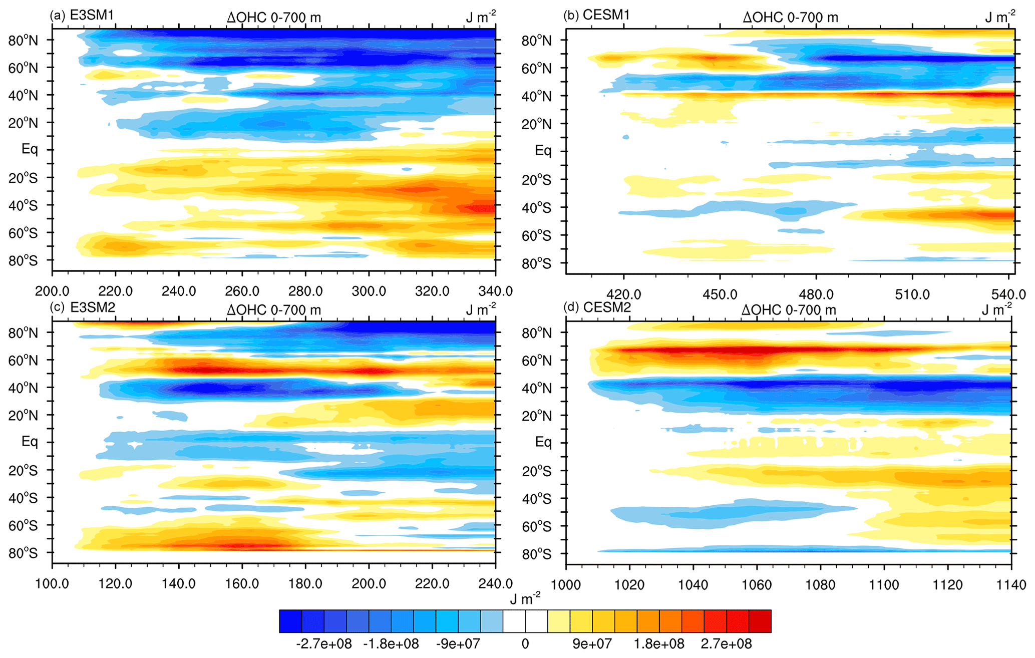
Figure 1Time–space evolution of ocean heat content changes in the preindustrial simulations for the top 700 m in the (a) E3SM1, (b) CESM1, (c) E3SM2, and (d) CESM2, respectively, after the approximate time of the ensemble initialization, which in some cases varies by ensemble member. Time intervals shown are chosen to correspond to 1850–1990 in the historical era. In cases of variable initialization dates, an approximate date range is chosen (1000 years for CESM2, 200 years for E3SM1, and 100 years for E3SM2). A 70-year running smoothing is applied to reduce internal variability.
Upper-ocean drift in CESM1 is also strong at some latitudes, with features that include a cooling north of 45° N and from 10° S to 20° N and weak drift at most other latitudes (Fig. 1b). Drift in the full-depth ocean is characterized by cooling generally north of 10° S and warming in the Southern Ocean (Fig. S3b). The sign of drift in the upper ocean in E3SM2 depends on latitude and is characterized generally by cooling in the Arctic and tropics and warming in the northern subtropics and Southern Ocean that largely offset each other in the global mean (Figs. 1c, S1, S2, S3c). At some latitudes, such as 40° N, the trends are not monotonic, with amplitudes that vary in time and change in sign and thus may instead be indicative of climate variability. Full-depth drift is characterized by cooling in the tropics and midlatitudes and warming at from 40 to 70° N, though such changes are again not monotonic in time (Fig. S3c). In CESM2, upper-ocean drift is also spatially complex (Fig. 1d), with a cooling drift from approximately 20–45° N, with slight warming at most other latitudes that grow over time. Drift in the full-depth ocean is characterized by a warming at nearly all latitudes that becomes particularly strong over time (Fig. S3d). The energy flux equivalents of these drifts, which are generally small, are shown in Fig. S4 to allow for comparison of drift magnitude to the radiative and energy flux responses shown in subsequent figures. The effects of these drifts are removed in all subsequent analyses based on the linear trends computed from the models' PI experiments during the period of overlap with the plotted fields. In instances in which multiple initialization dates exist across the ensemble, an average start date is used to define the period of overlap.
An analysis of global- and hemispheric-mean near-surface air temperature (T2 m) from 1850–2100 is shown in Fig. 2, with an analogous figure isolating historical era changes shown in Fig. S5. CESM1 has the coolest global-mean T2 m (286.3 K, Fig. 2a) during the base period (1920–50), while CESM2 has the warmest global-mean T2 m (287.2 K). Relative warmth across models in the PI simulation exhibits similar contrasts. Sufficient disagreement exists between the reanalysis datasets such that all models fall within the reanalysis range of base period T2 m (286.3 to 287.4 K). That said, the E3SM1 and E3SM2 are conspicuous for their lack of warming during the second half of the 20th century, in contrast to both reanalyses and CESM1/2. These biases and their drivers are addressed in Golaz et al. (2019, 2022) and further below and are shown to be the likely result of excessive cloud brightening due to sulfate aerosol–cloud interactions. Processes in the ocean may also play a role and are discussed further below. By 2100, the E3SM1 LE warms more than the other LEs, in part due to its high climate sensitivity (Zheng et al., 2022).
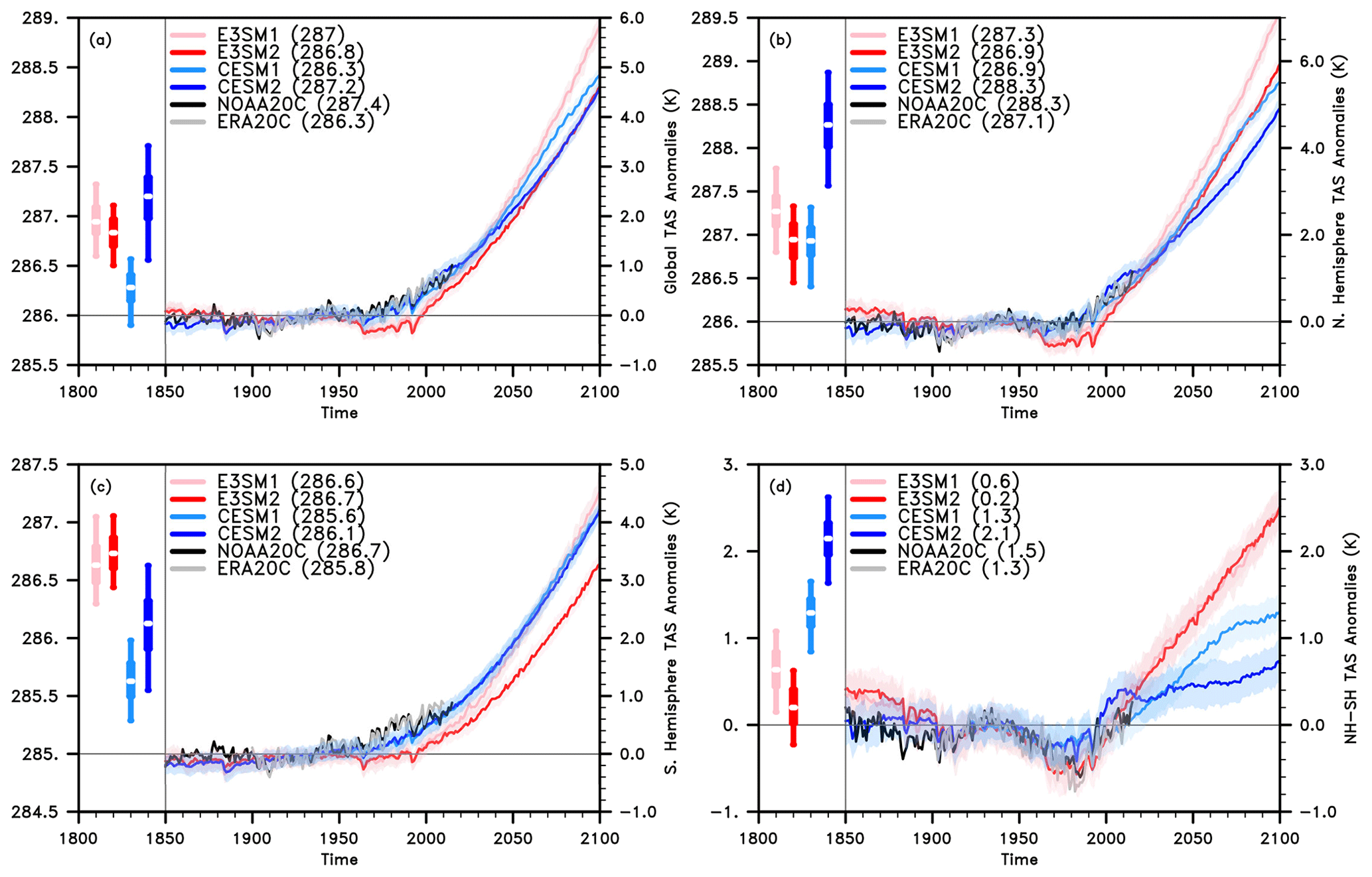
Figure 2Evolution of mean near-surface air temperature anomalies (K) for E3SM1/2 and CESM1/2 for (a) the globe, (b) the NH, (c) the SH, and (d) NH–SH, with drifts removed. The minimum, maximum, median, and interquartile range of annual means in the preindustrial simulations are also shown on the left axes. Observation-based estimates from NOAA20C (black) and ERA20C (grey) are indicated. A base period of 1920–1950 is used, and its values for each region are indicated in parentheses. All ensembles use the future SSP-3.70 scenario except CESM1 which uses RCP8.5.
Variability in T2 m in the PI experiment is larger in CESM2 than in the other models, (Fig. 2a, left inset), a likely result of its excessive ENSO variability (Fasullo et al., 2020). The NH is also considerably warmer in CESM2 during the base period and PI simulation than in the other models (Fig. 2b, left inset) though differences between the observations exceed 1 K, undermining definitive statements of model bias. Cooling in the 20th century is particularly strong in the NH in E3SM1/2 (Figs. 2b, S5b). In addition to the effects of sulfate aerosols (Golaz et al., 2019, 2022; Zheng et al., 2022), drift is also a potential contributor to the lack of NH warming in E3SM1 (Fig. 1a). In the SH (Fig. 2c), CESM1 is about a degree cooler than the other models, with both E3SM1 and E3SM2 exhibiting a warm SH in the PI simulation (Fig. 2c, left inset). Warming in the SH in the late 20th century in E3SM1/2 is also stronger than in the NH, though the SH warming is weaker than in reanalyses. The hemispheric gradient during the base period (1920–1950, Fig. 2d) is characterized by a NH that is warmer than the SH by about 1.5 K in reanalyses (values in parentheses). In the LEs this value varies greatly, as the NH is warmer than the SH in all cases, but hemispheric contrasts are too weak in E3SM1/2 (0.6, 0.2 K) and too strong in CESM2 (2.1 K) as compared to reanalyses.
Imbalances in the energy budget are a key driver of the FR, and the net TOM flux (RT, Fig. 3) is therefore a useful metric for assessing transient responses in the LEs. The E3SM and CESM LEs are generally in good balance during the PI, with absolute RT of ≤ 0.12 W m−2 (Fig. S2). As was the case for T2 m (Fig. 2a), variability is greater in CESM2 in RT than in other models (Fig. 3a, left inset), suggesting the influence of excessive ENSO variance. A small but positive RT (heating) is evident in all ensembles in the early 20th century, with episodic intervals of cooling due to volcanic eruptions (Fig. 3a). Ensemble-mean RT in all LEs from 2000–2020 (values in parentheses) is less than in CERES (black line), whose value is 1.1 W m−2, and RT is particularly small in E3SM2 (0.5 W m−2). Trends in RT in CERES are also much larger than in any of the LE ensemble means. While the influence of internal variability may drive deviations greater than the ensemble-mean trend, only 7 % and 5 % of the members in the E3SM1 and CESM1 LEs, respectively, have trends as large as CERES and no E3SM2 or CESM2 LE members exhibit trends as large, suggesting a contribution from errors in either prescribed forcings or model physics, as discussed further below.
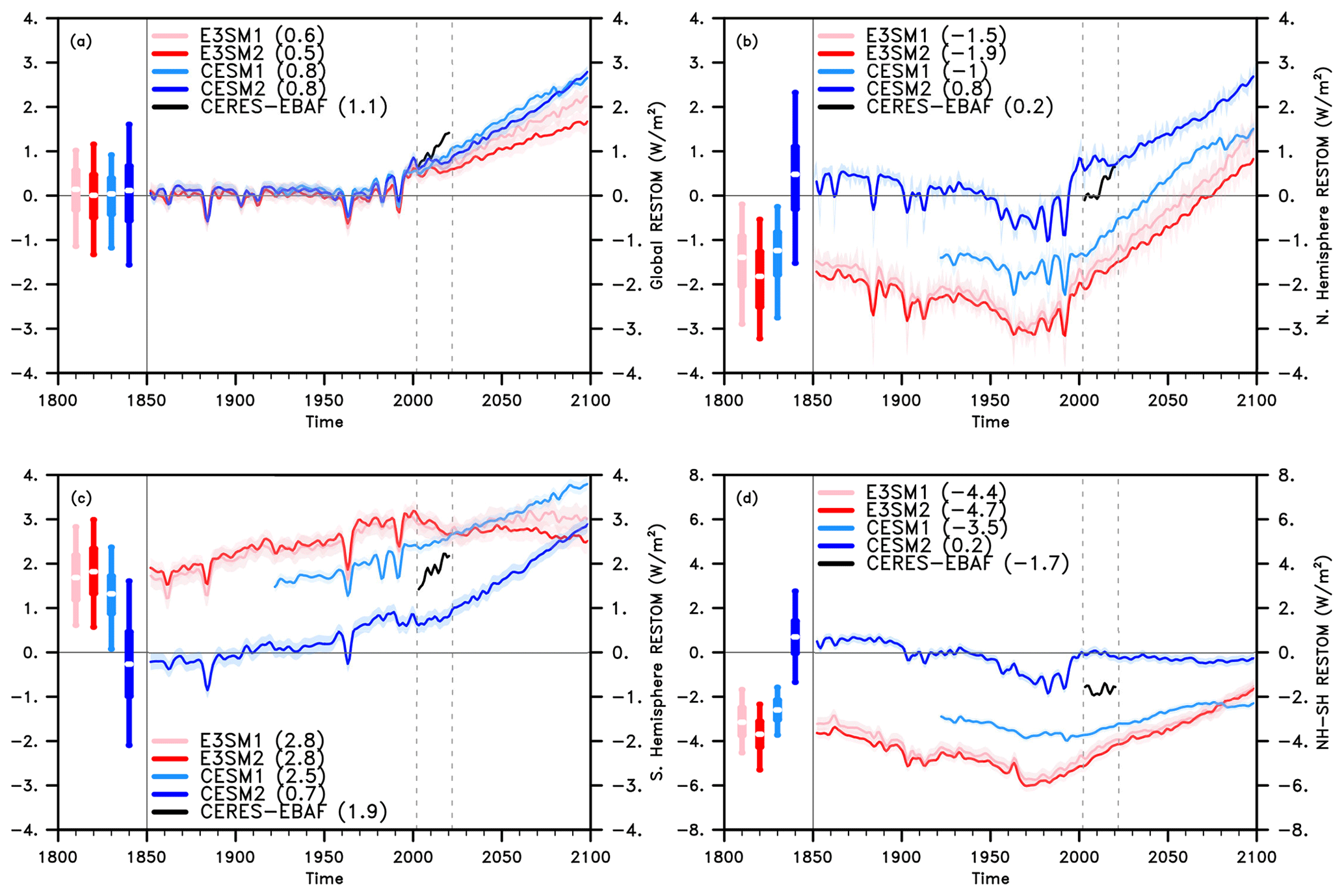
Figure 3Evolution of top-of-model net radiative flux (W m−2) for E3SM1/2, CESM1/2, and observations for 2000–2022 from CERES for (a) the globe, (b) the NH, (c) the SH, and (d) NH–SH, with drifts removed. The minimum, maximum, median, and interquartile range of annual means in the preindustrial simulations are also shown on the left axes. Values from CERES (black) are also shown. All ensembles use the future SSP-3.70 scenario, except CESM1, which uses RCP8.5.
The hemispheric energetic imbalance exerts an important influence on many aspects of climate, and so both the hemispheric means and their contrasts are also assessed in Fig. 3. Most volcanic eruptions exert a greater overall reduction in RT in the NH due to their tendency to occur in the tropics and NH, and asymmetries in the stratospheric circulation that enhance NH aerosol burdens even for tropical eruptions (Quaglia et al., 2023). This is evident for example in the transient signals in hemispheric differences, which are negative for most eruptions in the LEs, with the main exception being for the 1963 eruption of Mt. Agung in E3SM2 (Fig. 3d). Only CESM2 has a NH flux that is positive from 2000–2020, and among the LEs it agrees most closely with CERES. The existence of strongly negative NH RT, particularly in E3SM2 (−1.9 W m−2), may relate to excessive aerosol forcing (Golaz et al., 2022) but is likely also influenced by structural model bias (e.g., in clouds), as similar inter-model contrasts are evident in the PI simulations (Fig. 3b). Conversely, all models except CESM2 simulate SH RT that is larger than observed (Fig. 3c), though CESM2 is also biased as it simulates values that are too small. E3SM1 and E3SM2 have flat trends in RT in the 21st century but for different reasons. In E3SM1 the RT trend is flat because OLR and T2 m trends are stronger than in the other ensembles and thus offset SWTOA changes (Figs. 2, S7, S8). In E3SM2 the RT trend is flat because SWTOA trends are weak relative to the other ensembles (Fig. S8) and are thus offset by OLR trends. Contrasts between hemispheres (NH-SH, Fig. 3d) in CESM2 are weaker than observed but are larger than the other LEs, which are too negative, particularly in E3SM1/2, an issue explored in depth in Golaz et al. (2019, 2022).
The time–latitude structure of warming is shown in Fig. 4, and it exhibits many of the features anticipated from the global-scale time evolution of RT (Fig. 2). Common to the ensembles is a broadscale warming through 2100 that is greatest at high latitudes and is somewhat stronger in the Arctic than the Antarctic, consistent with the effects of Arctic amplification (Serreze et al., 2011). An additional feature of E3SM1/2 that is not evident in CESM1/2 is the strong 20th century cooling evident from 30–70° N (Fig. 4a, c), which is addressed in both Golaz et al. (2019, 2022) and Zheng et al. (2022) and attributed to an excessive cooling response to anthropogenic sulfate aerosols. Time series from single-forcing experiments support this interpretation, as the aerosol response in T2 m is found to be about twice as large in E3SM2 as in CESM2 (Fig. S6). Simulation drift is also a likely contributor to mid 20th century NH midlatitude cooling (Figs. 1, S3). The aerosol cooling signal is the first FR that emerges from the noise of internal variability in both E3SM1 (lack of stippling where significant in all figures) and E3SM2. In CESM1, the identification of emergent signals and differences with CESM2 prior to 1920 is not possible due largely to the availability of only a single ensemble member (stippling before 1920 in Fig. 4b, d). Instead, Arctic warming is the first forced response to emerge, which occurs shortly after the initialization of the ensemble in 1920 (Fig. 4b). Though somewhat delayed versus E3SM1, 20th century NH cooling in E3SM2 is stronger than in E3SM1 at most times and latitudes, particularly in the Arctic (as evident from the lack of stippling from 1920–2000 from 60–90° N in Fig. 4c). Warming in the mid to late 21st century (21C) is greater in E3SM1, which has an unrealistically large equilibrium climate sensitivity (Golaz et al., 2019). For CESM1/2, the large number of ensemble members after 1920 increases the detectability of intergenerational differences (lack of stippling in most regions of Fig. 4d). Though the general patterns of warming are similar, some differences are evident, such as the elevated future warming from 0–20° S in CESM2. Warming above 5 K in the NH also extends farther south in E3SM than in CESM. However, comparison between CESM1 and the other models is complicated by contrasts in prescribed climate forcings, with CESM1 using RCP85 and other LEs using SSP370.
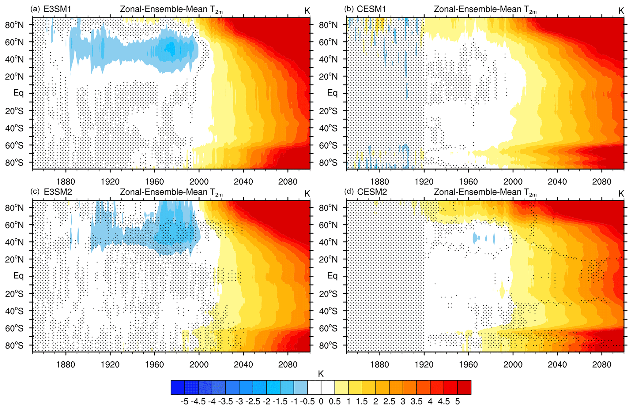
Figure 4Ensemble-mean change in 2 m air temperature (K) from the 1850–1859 average in E3SM1 (a), CESM1 (b), E3SM2 (c), and CESM2 (d), with drifts removed. Stippling indicates changes less than twice the standard error in (a) and (b) and inter-generational differences (e.g., E3SM1 versus E3SM2) less than twice the standard error in (c) and (d). All ensembles use the future SSP-3.70 scenario, except CESM1, which uses RCP8.5.
The time–latitude evolution of RT is a key indicator of the influence of forcing and is shown in Fig. 5. In E3SM1/2, the 20th century evolution is characterized by robust negative RT anomalies (cooling) that begin in the late 19th century from 30–70° N and that intensify into the late 20th century in conjunction with positive anomalies (heating) that emerge and intensify in the low-latitude SH (indicated by lack of stippling in Fig. 5a). Analysis of precipitation (to be discussed below in Fig. 8) shows the SH features to be related to displacements of tropical deep convection, consistent with the response to sustained NH cooling (Hwang and Frierson, 2013). While locations and timings of mid 20th century forced RT anomalies in CESM1/2 similar to those E3SMv1/2 are evident (e.g., lack of stippling in Fig. 5b), their magnitudes are weaker. Short-lived cooling pulses across a broad range of latitudes are also evident in all LEs, and these are driven by major volcanic eruptions. In the 21st century, the latitudinal structures of RT anomalies exhibit common features across the ensembles, including a broadscale heating that is greatest in the Arctic and a heating–cooling dipole south of 60° S. Other details in the structure, such as trends between 10 and 40° S, are strongly model dependent and likely relate to cloud responses to warming and adjustments to CO2, such as for example the rapid SH subtropical cloud adjustment to CO2 in CESM2 (Fasullo and Richter, 2023). Detectable differences between successive model generations are also evident at various times and latitudes (lack of stippling in Fig. 5c, d). In CESM, however, the interpretation of such differences is complicated by the potential role for contrasts in the forcing scenarios used for both the historical and future eras and therefore cannot be directly attributed to model version (Fasullo and Richter, 2023).
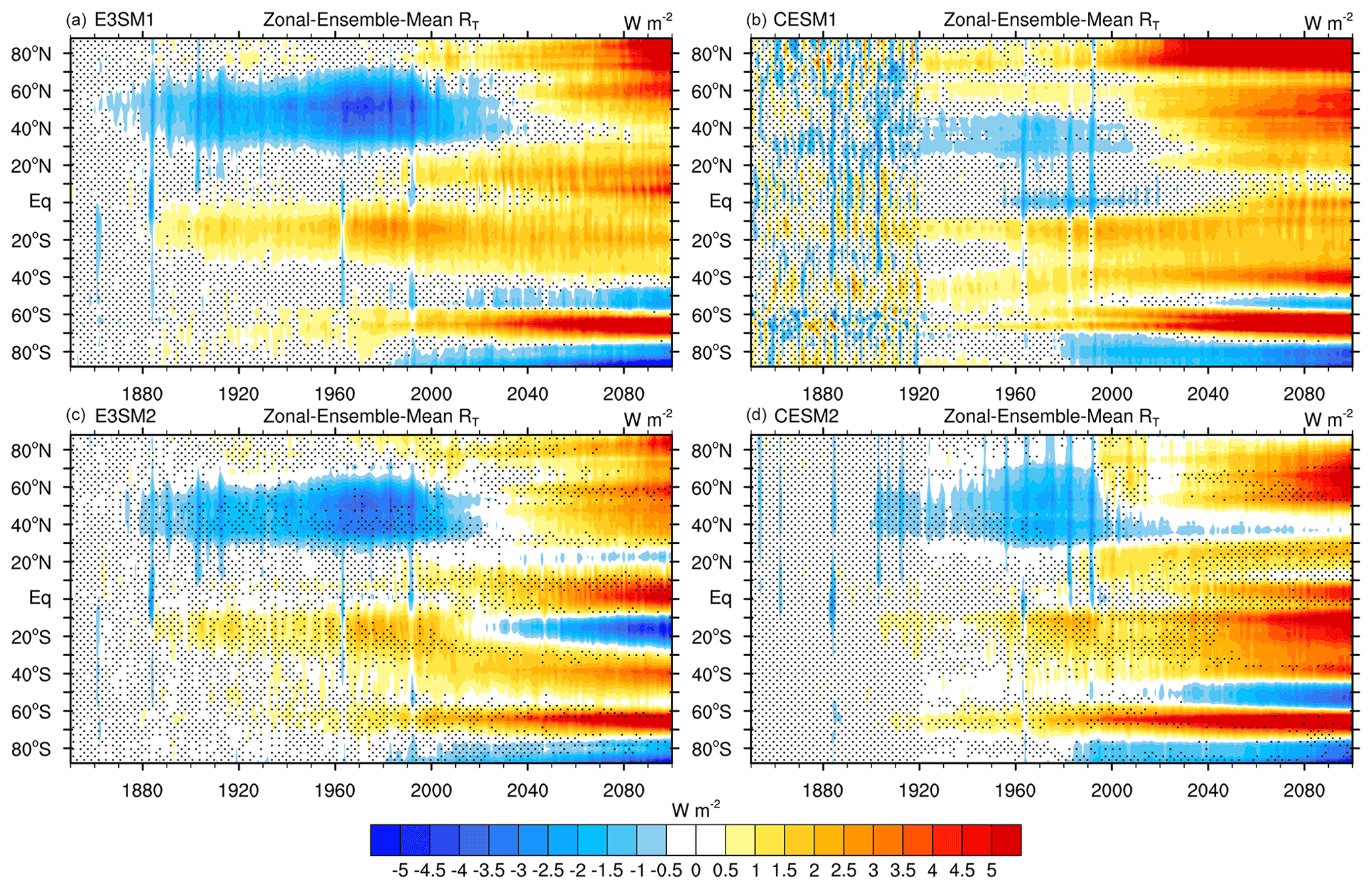
Figure 5Ensemble-mean change in net top-of-model radiation (W m−2) from the 1850–1859 average in E3SM1 (a), CESM1 (b), E3SM2 (c), and CESM2 (d), with drifts removed. Stippling indicates changes less than twice the standard error in (a) and (b) and intergenerational differences less than twice the standard error in (c) and (d). All ensembles use the future SSP-3.70 scenario except CESM1 which uses RCP8.5.
As dominant contributors to anomalies in RT and their differences across models, changes in SWTOM highlight important contrasts across the LEs. The time–latitude structure of SWTOM anomalies is shown in Fig. 6. In E3SM1/2 (Fig. 6a, c), the 20th century evolution is characterized by robust cooling anomalies that begin in the late 19th century from 30–70° N that intensify into the late 20th century, similar to anomalies in RT. Unlike RT anomalies, however, there is little change in SWTOM in the SH during the mid 20th century, suggesting a role for high clouds and reduced longwave fluxes tied to changes in deep convection in dictating changes in RT (Fig. 5). While episodes of negative forced anomalies in CESM1/2 in the 20th century are evident (e.g., lack of stippling in Fig. 6b), they are shorter lived and their magnitudes are significantly weaker than in E3SM1/2. An influence of volcanic eruptions is again evident in the episodic cooling pulses in the 20th century in all LEs (across many latitudes). In the 21st century, the latitudinal structure of SWTOM anomalies exhibit common features across the ensembles, such as a broadscale heating that is evident in the extratropics in all ensembles except at 60° S, where at times the signs of model trends disagree. Contrasts in the timing and magnitudes of projected changes are also evident across latitudes.
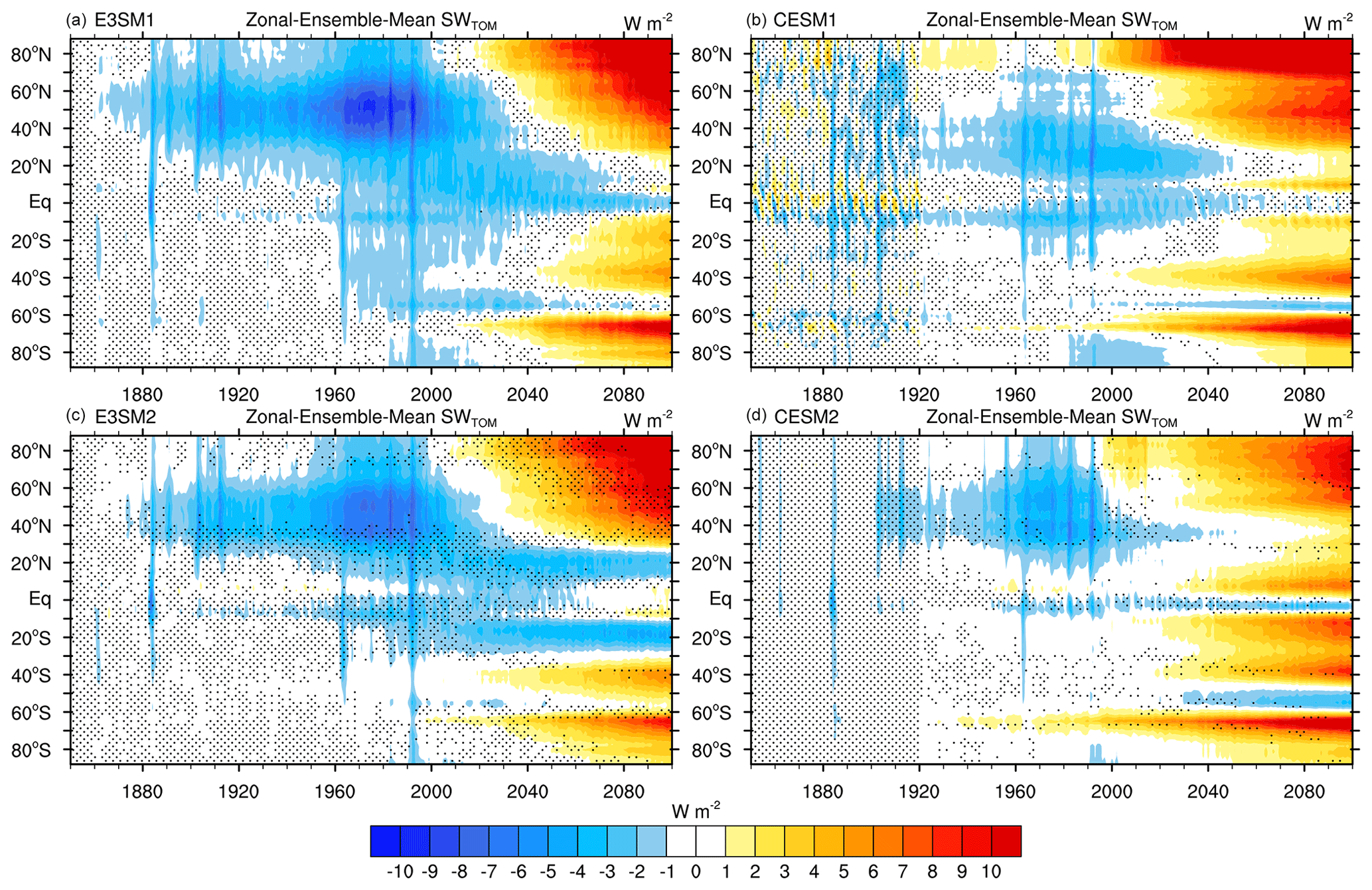
Figure 6Ensemble-mean change in net top-of-model absorbed shortwave radiation (W m−2) from the 1850–59 average in E3SM1 (a), CESM1 (b), E3SM2 (c), and CESM2 (d), with drifts removed. Stippling indicates changes less than twice the standard error in (a) and (b) and intergenerational differences less than twice the standard error in (c) and (d). All ensembles use the future SSP-3.70 scenario, except CESM1, which uses RCP8.5.
The effects of forced responses, such as the NH cooling in the mid to late 20th century and global warming in the 21st century, extend beyond temperature and include the water cycle due in part to the energetic linkages between these fields (Trenberth et al., 2009). Responses in the LEs in precipitable water (PrW), which is the integrated water vapor in the atmosphere expressed in liquid-equivalent depth, are shown in Fig. 7. With cooling, the capacity of air to hold moisture decreases, and forced reductions in PrW are therefore coincident in E3SM1/2 with periods of cooling across the NH in the mid 20th century. Forced reductions in E3SM1 (Fig. 7a) are first simulated in the late 19th century (coincident with the eruption of Krakatoa in 1883) and persist through the 20th century, reaching a peak intensity near 1 mm in the 1960s and 1970s. Reductions of similar intensity and timing are evident in E3SM2, and the PrW increases in the SH are coincident with enhancement of tropical precipitation (to be discussed further below). Responses in the 20th century are small, however, relative to projected increases in PrW in association with projected warming (Fig. 4), with increases that exceed 8 mm in the tropics and subtropics in all LEs by the late 21st century. Increases in PrW in CESM1/2 are first evident in the SH in the mid 20th century. In the 21st century, increases are approximately symmetric about the Equator in E3SM1 and CESM1/2 but are skewed toward the NH in E3SM2, where the greatest increases are located north of 20° S, consistent with the somewhat muted warming in E3SM2 (Fig. 4c) and a fixed relative humidity constraint. Increases south of 70° S are relatively small in all LEs, likely due to limitations on surface water availability and very low mean-state temperatures and PrW values over Antarctica.
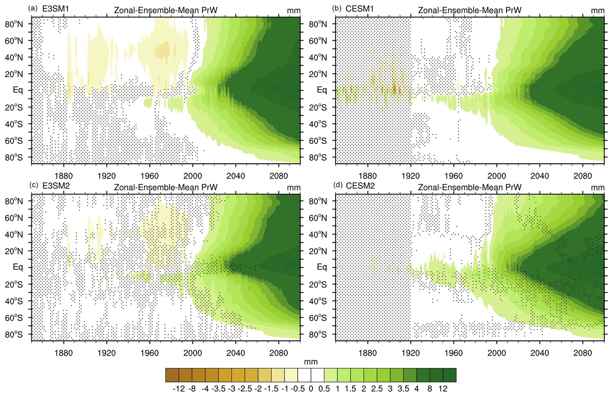
Figure 7Ensemble-mean change in precipitable water (mm) from the 1850–1859 average in E3SM1 (a), CESM1 (b), E3SM2 (c), and CESM2 (d), with drifts removed. Stippling indicates changes less than twice the standard error in (a) and (b) and intergenerational differences less than twice the standard error in (c) and (d). All ensembles use the future SSP-3.70 scenario, except CESM1, which uses RCP8.5.
The water cycle perturbation responses in PrW are associated with spatially complex responses in precipitation (P), shown in Fig. 8. With a cooler lower atmosphere (Fig. 4), less SW flux available at the surface to supply the energy consumed by evaporation (Fig. 6), and reduced PrW (Fig. 7), the NH climate in E3SM1/2 experiences significant forced reductions in P across the 20th century at all latitudes (Fig. 8a, c). In addition, the southward shift in deep convection in E3SM1/2 cited above is expressed as decreases in P in the tropics and increases in P from 5 to 20° S that peak in the 1970s. The spatial structure of anomalies during this time is characterized by particularly strong reductions in P in the western Pacific warm pool and NH deep convective regions and increases south of the Equator across much of the SH (not shown). Similar responses in P in CESM1/2 also emerge from background variability (Fig. 8b, d) but are weaker at most latitudes, particularly in CESM2, and do not extend as far north as in E3SM1/2. Projected changes are characterized by robust increases in P in all LEs on the Equator and in the middle to high latitudes, while decreases are projected in the subtropics generally, though with magnitudes, latitudinal bounds, and timings that vary across LEs.
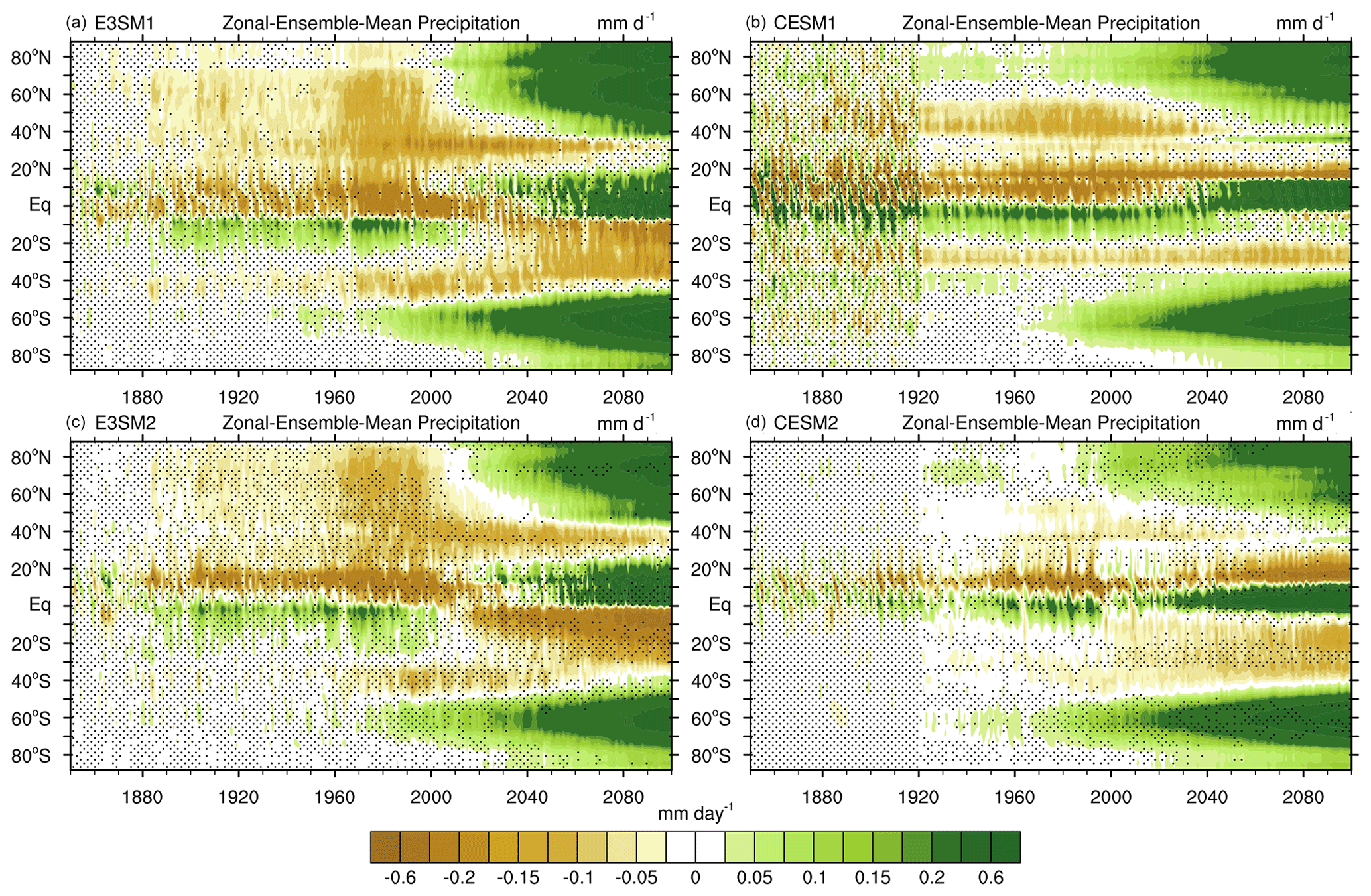
Figure 8Ensemble-mean change in precipitation (mm d−1) from the 1850–1859 average in E3SM1 (a), CESM1 (b), E3SM2 (c), and CESM2 (d), with drifts removed. Stippling indicates changes less than twice the standard error in (a) and (b) and intergenerational differences less than twice the standard error in (c) and (d). All ensembles use the future SSP-3.70 scenario, except CESM1, which uses RCP8.5.
Meridional atmospheric heat transports (MHTatm), defined as positive for northward transports, are strongly coupled to the latitudinal structures of thermal and moisture fields, and their forced changes are shown in Fig. 9. In E3SM1/2, increases in MHTatm are evident north of 20° S in the 20th century, which are particularly strong (> 0.1 PW) from 1960–2000 and coincide with strong aerosol-induced cooling (Figs. 4–6). The initial emergence of forced increases in E3SM occurs in the late 19th century. The increased meridional thermal gradient arising from aerosol forcing is a likely contributor to the mid to late 20th century MHTatm maximum (Needham et al., 2023). Changes in CESM during the 20th century are weak compared to those in E3SM, with increases near 0.08 PW at low latitudes. In the 21st century, changes are characterized by increased poleward transport of order 0.2 PW, characterized by positive (negative) MHTatm in the NH (SH), but with strong hemispheric and model dependence. Increases in MHTatm in the NH are weak in E3SM1 and largely absent from E3SM2 (Fig. 9a, c), likely due to the disproportionately strong 21st century surface warming in the NH (Fig. 4) and the associated weakening of the meridional temperature gradient. Projected MHTatm increases in the NH are particularly pronounced in CESM2 and are in part associated with the large projected increase in RT and SWTOM near 20° S, which contributes to increased low-latitude atmospheric energy divergence (Fig. 6d).
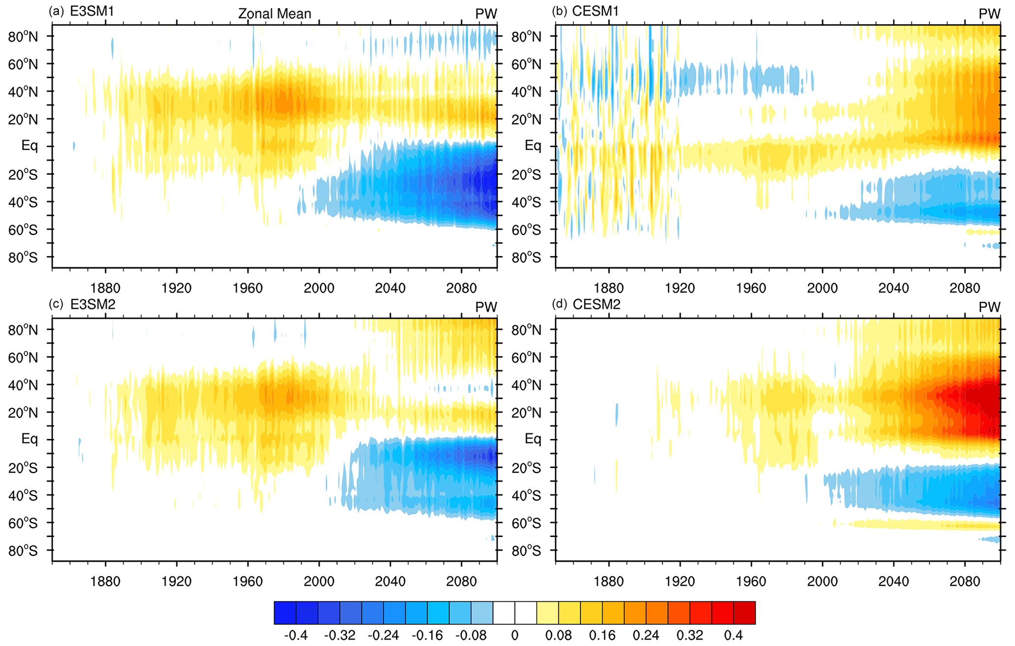
Figure 9Ensemble-mean change in meridional atmospheric heat transport (PW) from the 1850–1859 average in E3SM1 (a), CESM1 (b), E3SM2 (c), and CESM2 (d), with drifts removed. Stippling indicates changes less than twice the standard error in (a) and (b) and intergenerational differences less than twice the standard error in (c) and (d). All ensembles use the future SSP-3.70 scenario, except CESM1, which uses RCP8.5.
Meridional oceanic heat transports (MHTocn) exert an influence that is generally strongest equatorward of 30° N/S in the climatological mean (Trenberth and Fasullo, 2017), and their forced changes are shown in Fig. 10. In E3SM1/2, increases in MHTocn are evident north of 20° S in the 20th century, which are particularly strong (> 0.2 PW) from 1960–2000 and, as with MHTatm, coincide with strong aerosol-induced cooling (Figs. 4–6). Changes in CESM1/2 in the 20th century are relatively weak, with increases near 0.05 PW from 1960–2000. In the 21st century, forced reductions in poleward MHTocn are evident in all LEs but with strong model dependence and large magnitudes in CESM and particularly in CESM1. Projected decreases in the NH are likely tied to changes in the Atlantic Meridional Overturning Circulation (AMOC) and the lack of strong NH decreases in E3SMv1/2 may reflect weak AMOC conditions in the present-day (Hu et al., 2020) and the associated limited potential for future weakening.
Figure 10Ensemble-mean change in meridional ocean heat transport (1015 W) from the 1850–1859 average in E3SM1 (a), CESM1 (b), E3SM2 (c), and CESM2 (d), with drifts removed. Stippling indicates changes less than twice the standard error in (a) and (b) and intergenerational differences less than twice the standard error in (c) and (d). All ensembles use the future SSP-3.70 scenario, except CESM1, which uses RCP8.5.
As the ocean stores over 90 % of Earth's energy imbalance, model dependence in climate system storage is reflected in contrasts in ocean heat content (OHC) trends, and these are shown for the surface to 2000 m depth in Fig. 11. Changes in OHC are small in the 19th century, although CESM1 and E3SM1 exhibit detectible cooling by 1900 and are notably cooler than CESM2 and E3SM2 by 1950. In E3SM1 and E3SM2, the evolution of OHC after 1950 is quite different than in CESM, with strong cooling through the late 20th century, consistent with the aerosol effects already identified. Significant contrasts between models are also evident in the 21st century, with OHC increases in CESM1/2 being significantly greater than in E3SM1/2. The weak heat uptake in E3SM1/2, despite being associated with comparable surface warming (e.g., Figs. 2, 4), is likely to be linked with a weak AMOC in the models, with the effect of decreasing heat uptake by the deep ocean, consistent with the findings of Hu et al. (2020) for E3SM1 which linked the model's high transient climate response to weakness in AMOC. This lack of heat uptake and its associated weak ocean heat uptake efficacy may also play a role in amplifying the excessive surface cooling response to aerosol effects in the mid 20th century. Though transient climate response decreased in E3SM2 from E3SM1, it remains much larger than in either CESM1 or CESM2. This lack of ocean heat uptake in E3SM1 and E3SM2 may in turn contribute to strong 21st century NH warming (Fig. 4) and small changes in MHTatm (Fig. 9).
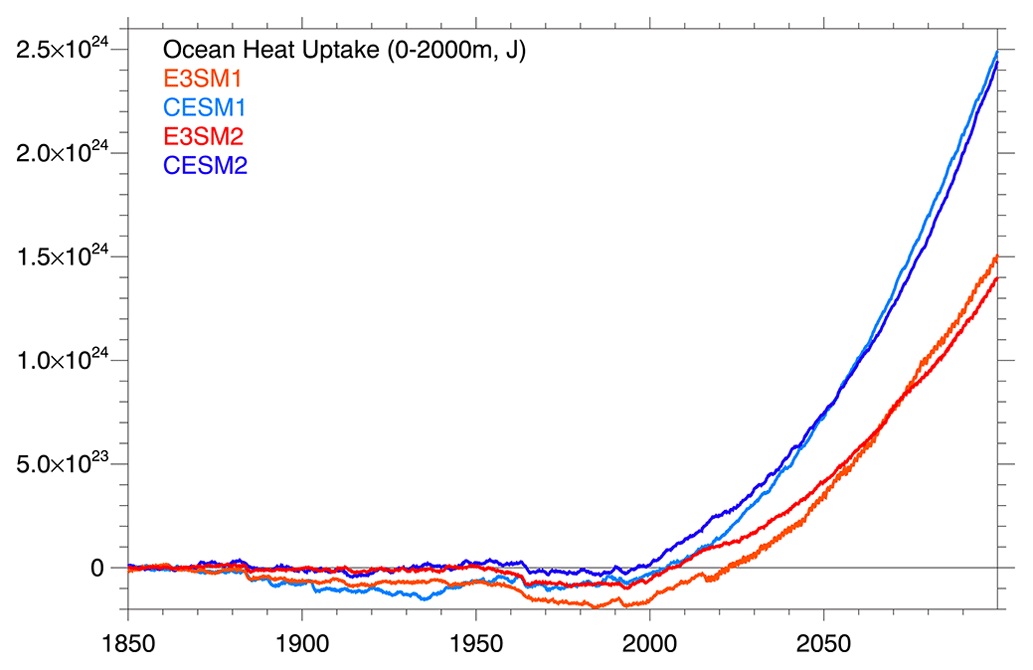
Figure 11Ensemble-mean zonal-mean ocean heat content change (J) from the surface to 2000 m versus the 1850–1859 average in E3SM1 (a), CESM1 (b), E3SM2 (c), and CESM2 (d). Drifts have been removed from each time series.
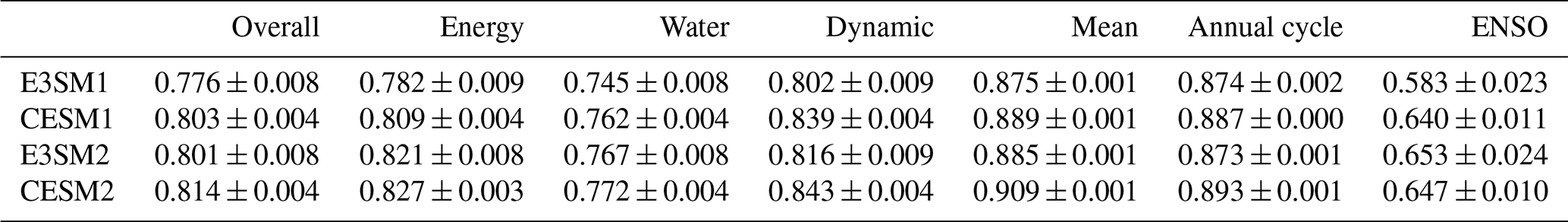
Summary scores for the model benchmarking tool CMATv1 (Fasullo, 2020), which compares global patterns of simulated dynamic, energy budget, and water cycle fields to satellite and reanalysis estimates, are shown in Table 1. Scores are based on pattern correlations for the climatological mean state, seasonal contrasts (June, July, August minus December, January, February mean states), and ENSO teleconnection patterns and therefore range from −1 (worst) to 1 (best). Multiple fields are considered for the energy budget (RT, SWTOM, OLR, shortwave and longwave cloud forcing, atmospheric energy divergence, and net surface heat flux), the water cycle (P, PrW, near-surface relative humidity, latent heat flux, and atmospheric moisture divergence), and dynamics (sea level pressure; near-surface wind speed; and eddy geopotential, relative humidity, and vertical velocity at 500 hPa). In the CMATv1 design, internal variability in the benchmarking metrics is designed to achieve specific known thresholds based on analysis of the CESM1 LE. The scores provide a range of insights into inter-model and inter-generational differences in the LEs and their significance, something also demonstrated for the CMIP ensembles in Fasullo (2020), where progressive improvement across model generations is identified. First, E3SM1 is generally the lowest-scoring model of the four, both in terms of the overall score (0.776) and more targeted scores in Table 1. E3SM1 scores particularly poorly in depicting ENSO teleconnections (0.583). Major improvements in E3SM2 from E3SM1 are apparent in the energy budget (from 0.782 to 0.821), water cycle scores (from 0.745 to 0.767), and ENSO teleconnections (from 0.583 to 0.653), which is the highest of the LEs assessed here (though within the uncertainty ranges of both CESM1 and CESM2). Scores for other summary metrics are highest for CESM2, and its improvements from CESM1 are evident in all metrics.
Table 1CMATv1 summary metrics (Fasullo, 2020) for E3SM1, CESM1, E3SM2, and CESM2 ensembles, with twice the ensemble standard error indicated. The scores are based on the global pattern correlations of 63 simulated fields with satellite and reanalysis estimates over recent decades. Examples of fields include TOA radiative fluxes, atmospheric energy divergence, precipitation, net surface heat flux, and 500 hPa eddy geopotential. Overall scores differing by 0.01 for the ensembles exceed the likely influence of internal variability.
To illustrate examples of simulated biases relevant to the CMATv1 benchmarks in Table 1 and the differences between E3SM1/2 and CESM1/2, biases in annual-mean RT are shown in Fig. 12. The biases are important as they influence the spatial gradients of temperature and moisture and thereby impact dynamics and MHT. Biases in E3SM1 and CESM1 are widespread in tropical and NH ocean regions, with RT that is too small. Exceptions include the regions of stratocumulus cloud decks west of Mexico and Peru, where RT is generally too large due to excess SW absorption and associated with deficient stratocumulus cloud decks (not shown). Over land, RT biases are generally positive, except in equatorial Africa, southern India, and South America, where it is often biased low, particularly in CESM1. Low biases are evident in the Tibetan Plateau in E3SM1 and E3SM2, which are not evident in CESM. The lowest root-mean-squared error (RMSE) in RT is found for CESM2 (7.8 W m−2), where regional biases are smaller than in CESM1 and E3SM1/2, while the highest RMSE is found for CESM1 (11.2 W m−2). The location of widespread ocean biases in CESM2 has also shifted to be largest near 50° S, where it is underestimated, while the other models tend to overestimate RT in the region.
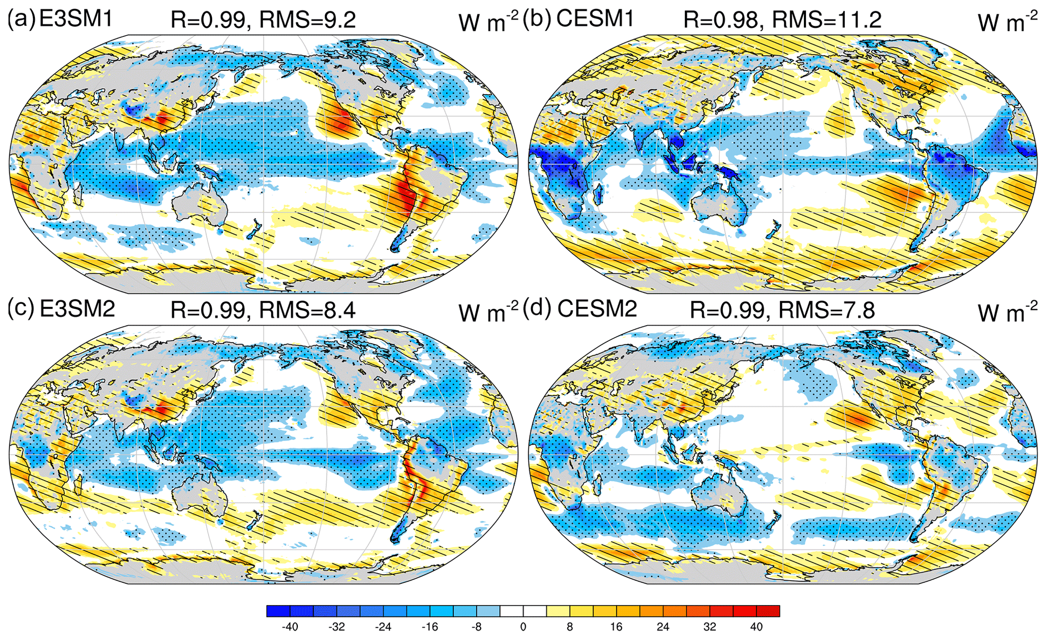
Figure 12Climatological ensemble-mean (2000–2020) net top-of-model radiation (RT) biases relative to CERES estimates from E3SM1 (a), CESM1 (b), E3SM2 (c), and CESM2 (d). Pattern correlation (r) and root-mean-squared error (RMSE) between the models and CERES are also shown in the title of each panel. Hatching and stippling corresponds to biases greater than 10 W m−2 and less than −10, W m−2, respectively.
Biases in precipitation (P) identified in CMATv1 for climatological-mean fields from 1979–2020, based on comparison against precipitation estimates from the Global Precipitation Climatology Project (Huffman et al. 2018), are shown in Fig. 13. In all ensembles a common pattern of biases exists, characterized by excess P in the off-equatorial Pacific Ocean (characteristic of the ubiquitous double Inter-Tropical Convergence Zone issue) and the western Pacific warm pool and deficient P in the equatorial Pacific Ocean and over much of South America. Pattern correlations improve slightly from versions 1–2 of both E3SM (0.88 to 0.85) and CESM (0.85 to 0.89), and RMSE is lowest for E3SM2 and CESM2 (0.99), due largely to reduced biases in the southeastern subtropical Pacific Ocean.
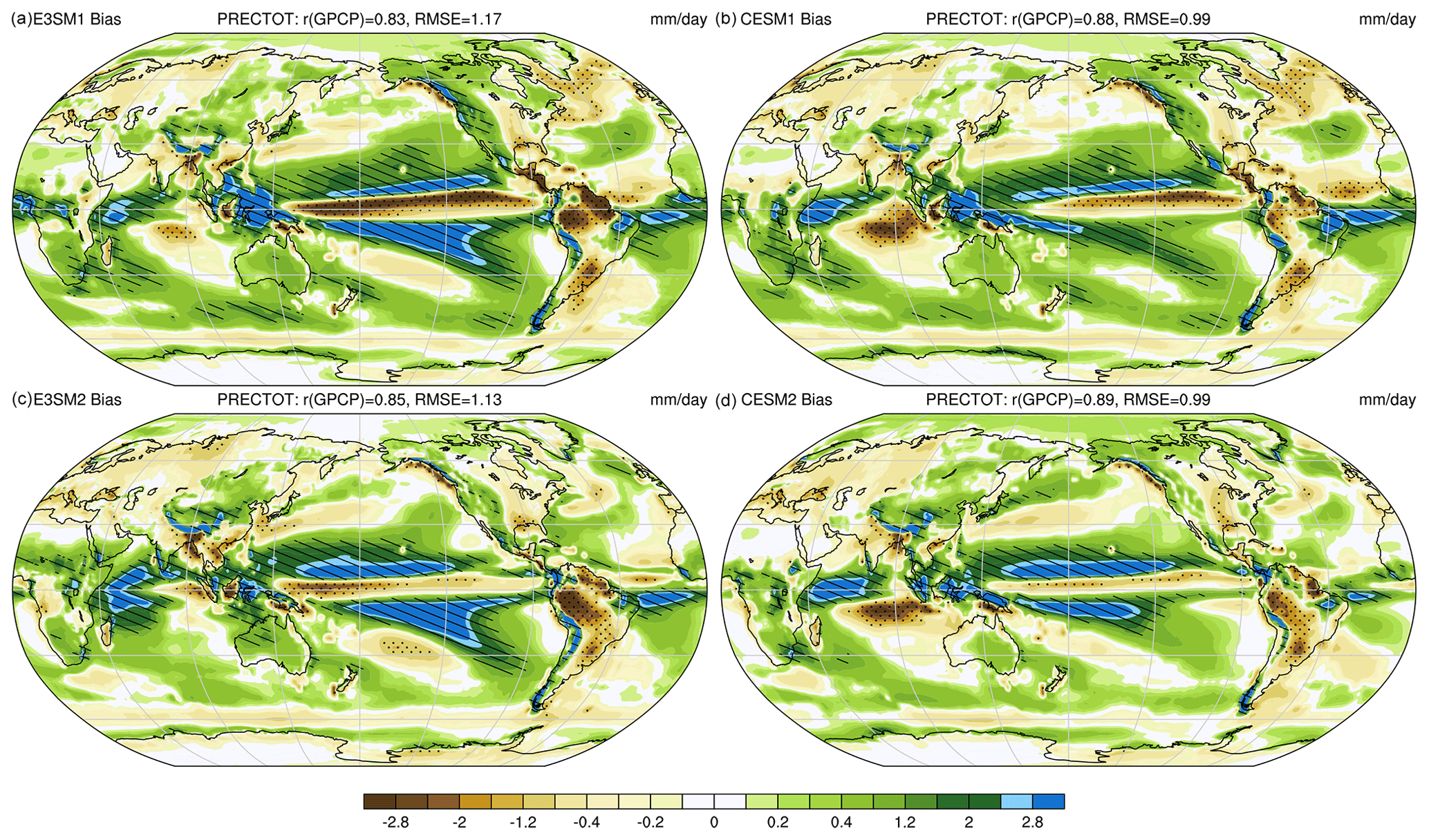
Figure 13Climatological ensemble-mean (1979–2020) precipitation biases relative to GPCP estimates from E3SM1 (a), CESM1 (b), E3SM2 (c), and CESM2 (d). Pattern correlation (r) and root-mean-squared error (RMSE) between the models and GPCP are also indicated in the title of each panel. Hatching and stippling corresponds to biases greater than 1 mm d−1 and less than −1 mm d−1, respectively.
Finally, the sensitivity of E3SM2 to CMIP6 prescribed emissions is explored in Fig. 14. In Fasullo et al. (2022), a sensitivity in CESM2 to these emissions was shown to drive a strong high-latitude warming, owing to an abrupt increase in emission variability in 1997 that via nonlinear interactions with clouds drove a rectified reduction in mean albedo from 40–70° N. Here, based on the ensemble mean differences between the E3SM2 LE and smoothed biomass LE it is shown further that E3SM2 exhibits a similar, albeit somewhat weaker, response. The response is characterized for example by reductions in cloud albedo (Fig. 14a) and increases in T2 m (Fig. 14b), SWTOM (Fig. 14c), and surface net SW flux (SWSFC Fig. 14d), albeit with magnitudes that are reduced somewhat from those in CESM2 (dashed). These net reductions correspond to extremes in biomass emissions, which are particularly high in 1998 and 2003 and relatively low in most other years (see Fasullo et al., 2022, Fig. 1f). These variations result in radiation and T2 m anomalies that are negative during years of high emissions but positive and of comparable magnitude during the more frequent years of low emissions and thus drive a net warming. The spatial structure of the warming (Fig. 14e) is characterized by the strongest responses over NH land and the Arctic Ocean, where a warming response up to 0.5 K is simulated. Details of the interactions between emissions, clouds, radiation, and the broader climate state will be addressed in follow-up work.
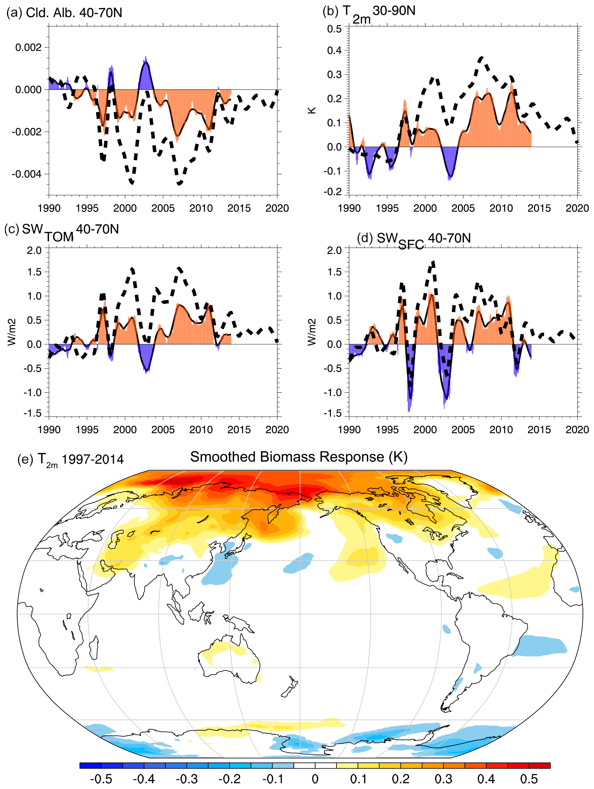
Figure 14Monthly (bars) and 12-month running-mean (solid line) ensemble-mean responses to variable biomass emissions in E3SM2 for (a) cloudy-sky albedo, (b) T2 m, (c) SWTOM, and surface net shortwave flux (SWSFC) (d). The associated sensitivities of CESM2 (12-month running mean) are also shown (dashed lines). (e) The spatial pattern of warming in response to CMIP6 biomass emissions (versus smoothed).
The unique value of LEs, which includes the opportunity to estimate forced climate responses and make robust comparisons across models, is illustrated in this work. In doing so, the LEs provide estimates of the potentially predictable component of the climate response arising from changes in its external forcings, which include most prominently industrial sulfate aerosols in the 20th century and greenhouse gases in the 20th century and 21st century, and allow for an assessment of inter-model contrasts. Understanding these structural uncertainties provides insight for interpreting historical era changes in nature and for quantifying the range of plausible 21st century climate outcomes, the factors underlying their differences, and associated uncertainties in a changing climate.
In this work, four recently produced LEs are intercompared and assessed with reanalysis and satellite datasets. The analysis summarizes many features of agreement in simulated climate across the LEs, which include a mid 20th century cooling driven by aerosols and an associated water cycle response, a polar amplification of warming and associated albedo reductions, increases in PW across latitudes, and latitudinally complex changes in P. Areas of disagreement across the LEs arising from contrasts in both model structure and imposed forcings, include contrasts in the magnitudes of mid to late 20th century cooling, the structure of associated low-latitude P responses, and changes in MHT. The contrast that exists in climate forcings used in CESM1 versus the other LEs limits strict statements regarding some of the comparisons made, for both historical (e.g., smoothed biomass) and future climates, and highlights the uncertainties associated with climate forcing agents (Fyfe et al., 2021; Holland et al., 2024).
In benchmarking the ensembles, robust improvements in E3SM and CESM are identified in the progression from versions 1 to 2. These improvements are particularly large in the energy budget and water cycles of E3SM and in its simulated ENSO teleconnections. The analysis also identifies a sensitivity in E3SM2 to the variable nature of CMIP6 biomass emissions similar to, but somewhat weaker than, that identified in CESM2 in prior work. Caution should therefore be exercised in evaluating transient climate features of the satellite era in both CESM2 and E3SM2. The failure of E3SM1 and E3SM2 to adequately warm during the late 20th century is also found to be a major shortcoming of the ensemble, with impacts on their simulation of the water cycle, and this feature is attributed to the models' excessive sensitivity to industrial sulfate aerosols and a secondary contribution from model drift. A notable interhemispheric contrast in drift is also identified for E3SM1. In comparison against CERES data during the early 21st century, very few LE members from any of the ensembles are found to exhibit trends in RT as large as observed from CERES, thus motivating further study on the origin of this apparent disagreement. Lastly, it is also noted that despite both being high-scoring models, E3SM2 and CESM2 project very different forced responses of radiation, precipitation, and meridional heat transport in both the atmosphere and ocean, underscoring the challenges that exist in narrowing future projections from evaluation with present-day observations alone. Work is ongoing to improve the sensitivity of the E3SM model to anthropogenic aerosol effects and better reproduce historical observations. The production of a large ensemble with this improved version is planned, and along with planned large ensembles and single-forcing ensembles in CESM and other climate models, will allow for a deeper understanding of the influences of climate drivers in both the historical and future eras and the inter-model contrasts in physics that govern the responses to them.
The CMATv1 code has been made available in Fasullo (2020).
The data for this study are available on the National Energy Research Scientific Computing Center Portal (https://portal.nersc.gov/archive/home/c/ccsm/www/E3SMv2/FV1/atm/proc/tseries/month_1, E3SM Project, 2024a) and Earth System Grid (e.g., https://aims2.llnl.gov/search/?project=E3SM/, E3SM Project, 2024b and https://aims2.llnl.gov/search/?project=CESM/, CESM Project, 2024a, b). The CERES data can be accessed at https://ceres.larc.nasa.gov/data/ (Clouds and the Earth's Radiant Energy System, 2024). NOAA 20th century reanalysis data are available at https://psl.noaa.gov/data/20thC_Rean/ (NOAA, 2015), while ERA 20th century reanalysis data are available at https://www.ecmwf.int/en/forecasts/dataset/ecmwf-reanalysis-20th-century (ECMWF, 2016). GPCP Climate Data Record precipitation is available at https://www.ncei.noaa.gov/access/metadata/landing-page/bin/iso?id=gov.noaa.ncdc:C00979 (GPCP, 2024).
The supplement related to this article is available online at: https://doi.org/10.5194/esd-15-367-2024-supplement.
JTF and JMC designed the study. JTF and JMC carried out the analysis and drafted the first version of the manuscript. All authors contributed to structuring the analysis and reviewing the manuscript. HW created model inputs of CMIP6 historical and future (SSP370) aerosol emissions for E3SM.
The contact author has declared that none of the authors has any competing interests.
Publisher's note: Copernicus Publications remains neutral with regard to jurisdictional claims made in the text, published maps, institutional affiliations, or any other geographical representation in this paper. While Copernicus Publications makes every effort to include appropriate place names, the final responsibility lies with the authors.
Portions of this study were supported by the Regional and Global Model Analysis (RGMA) component of the Earth and Environmental System Modeling Program of the U.S. Department of Energy's Office of Biological and Environmental Research (BER) under award no. DE-SC0022070 and by the National Center for Atmospheric Research, which is a major facility sponsored by the National Science Foundation (NSF) under cooperative agreement no. 1852977. The development of the E3SM model is supported by the E3SM project funded by the Office of Biological and Environmental Research in the U.S. Department of Energy's Office of Science. The efforts of John T. Fasullo in this work were also supported by NASA award nos. 80NSSC17K0565 and 80NSSC22K0046 and by NSF award no. 2103843. Work at LLNL was performed under the auspices of the U.S. Department of Energy by Lawrence Livermore National Laboratory under contract no. DE-AC52-07NA27344. This research used resources of the National Energy Research Scientific Computing Center (NERSC), a DOE Office of Science User Facility supported by the Office of Science of the U.S. Department of Energy under contract no. DE-AC02-05CH11231 using NERSC award no. ALCC-ERCAP0022631. The Pacific Northwest National Laboratory is operated for DOE by Battelle Memorial Institute under contract DE-AC05-76RL01830.
The efforts of John T. Fasullo in this work were supported by NASA award nos. 80NSSC21K1191, 80NSSC17K0565, and 80NSSC22K0046, and by the Regional and Global Model Analysis (RGMA) component of the Earth and Environmental System Modeling Program of the U.S. Department of Energy's Office of Biological and Environmental Research (BER) under award no. DE-SC0022070. This work also was supported by the National Center for Atmospheric Research, which is a major facility sponsored by the U.S. National Science Foundation (NSF) under cooperative agreement no. 1852977. John T. Fasullo was also supported by NSF award no. 2103843.
This paper was edited by Andrey Gritsun and reviewed by two anonymous referees.
CESM Project: Community Earth System Model Version 1 Large Ensemble, National Center for Atmospheric Research [data set], https://www.earthsystemgrid.org/dataset/ucar.cgd.ccsm4.cesmLE.html, last access: 3 April 2024a.
CESM Project: Community Earth System Model Version 2 Large Ensemble, National Center for Atmospheric Research [data set], https://www.earthsystemgrid.org/dataset/ucar.cgd.cesm2le.output.html, last access: 2 April 2024b.
Clouds and the Earth's Radiant Energy System: (CERES) radiative fluxes [data set], https://ceres.larc.nasa.gov/data/ (NASA/LARC/SD/ASDC, 2023), last access: 2 April 2024.
Compo, G. P., Whitaker, J. S., Sardeshmukh, P. D., Matsui, N., Allan, R. J., Yin, X., Gleason, B. E., Vose, R. S., Rutledge, G., Bessemoulin, P., Brönnimann, S., Brunet, M., Crouthamel, R. I., Grant, A. N., Groisman, P. Y., Jones, P. D., Kruk, M. C., Kruger, A. C., Marshall, G. J., Maugeri, M., Mok, H. Y., Nordli, Ø., Ross, T. F., Trigo, R. M., Wang, X. L., Woodruff, S. D., and Worley, S. J.: The twentieth century reanalysis project, Q. J. Roy. Meteorol. Soc., 137, 1–28, https://doi.org/10.1002/qj.776, 2011.
Danabasoglu, G., Lamarque, J.-F., Bacmeister, J., Bailey, D. A., DuVivier, A. K., Edwards, J., Emmons, L. K., Fasullo, J., Garcia, R., Gettelman, A., Hannay, C., Holland, M. M., Large, W. G., Lauritzen, P. H., Lawrence, D. M., Lenaerts, J. T. M., Lindsay, K., Lipscomb, W. H., Mills, M. J., Neale, R., Oleson, K. W., Otto-Bliesner, B., Phillips, A. S., Sacks, W., Tilmes, S., van Kampenhout, L., Vertenstein, M., Bertini, A., Dennis, J., Deser, C., Fischer, C., Fox-Kemper, B., Kay, J. E., Kinnison, D., Kushner, P. J., Larson, V. E., Long, M. C., Mickelson, S., Moore, J. K., Nienhouse, E., Polvani, L., Rasch, P. J., and Strand, W. G.: The Community Earth System Model V ersion 2 (CESM2), J. Adv. Model. Earth Sy., 12, e2019MS001916, https://doi.org/10.1029/2019MS001916, 2020.
Deser, C., Lehner, F., Rodgers, K. B., Ault, T., Delworth, T. L., DiNezio, P. N., Fiore, A., Frankignoul, C., Fyfe, J. C., Horton, D. E., Kay, J. E., Knutti, R., Lovenduski, N. S., Marotzke, J., McKinnon, K. A., Minobe, S., Randerson, J., Screen, J. A., Simpson, I. R., and Ting, M.: Insights from Earth system model initial-condition large ensembles and future prospects, Nat. Clim. Change, 10, 277–286, https://doi.org/10.1038/s41558-020-0731-2, 2020.
E3SM Project: Energy Exascale Earth System Model Version 2 Large Ensemble, Department of Energy [data set], https://portal.nersc.gov/archive/home/c/ccsm/www/E3SMv2/FV1/, last access: 2 April 2024a.
E3SM Project: Energy Exascale Earth System Model Version 1 Large Ensemble, Department of Energy [data set], https://portal.nersc.gov/archive/home/c/ccsm/www/E3SMv1-LE/FV1, last access: 2 April 2024b.
ECMWF (European Centre for Medium-Range Weather Forecast): ERA20C reanalysis data [data set], https://apps.ecmwf.int/datasets/data/era20c-moda/levtype=sfc/type=an/ (last access: 2 April 2024), 2016.
Eyring, V., Bony, S., Meehl, G. A., Senior, C. A., Stevens, B., Stouffer, R. J., and Taylor, K. E.: Overview of the Coupled Model Intercomparison Project Phase 6 (CMIP6) experimental design and organization, Geosci. Model Dev., 9, 1937–1958, https://doi.org/10.5194/gmd-9-1937-2016, 2016.
Fasullo, J. T.: Evaluating simulated climate patterns from the CMIP archives using satellite and reanalysis datasets using the Climate Model Assessment Tool (CMATv1), Geosci. Model Dev., 13, 3627–3642, https://doi.org/10.5194/gmd-13-3627-2020, 2020.
Fasullo, J. T. and Nerem, R. S. Altimeter-era emergence of the patterns of forced sea-level rise in climate models and implications for the future, P. Natl. Acad. Sci. USA, 115, 12944–12949, 2018.
Fasullo, J. T., Otto-Bliesner, B. L., and Stevenson, S.: ENSO's changing influence on temperature, precipitation, and wildfire in a warming climate, Geosci. Res. Lett., 45, 9216–9225, 2018.
Fasullo, J. T., Phillips, A. S., and Deser, C.: Evaluation of leading modes of climate variability in the CMIP archives, J. Clim., 33, 5527–5545, https://doi.org/10.1175/JCLI-D-19-1024.1, 2020.
Fasullo, J. T., Lamarque, J. F., Hannay, C., Rosenbloom, N., Tilmes, S., DeRepentigny, P., Jahn, A., and Deser, C.: Spurious late historical-era warming in CESM2 driven by prescribed biomass burning emissions, Geosci. Res. Lett., 49, e2021GL097420, https://doi.org/10.1029/2021GL097420, 2022.
Fasullo, J. T. and Richter, J. H.: Dependence of strategic solar climate intervention on background scenario and model physics, Atmos. Chem. Phys., 23, 163–182, https://doi.org/10.5194/acp-23-163-2023, 2023.
Frankignoul, C., Gastineau, G., and Kwon, Y.-O.: Estimation of the SST Response to Anthropogenic and External Forcing and Its Impact on the Atlantic Multidecadal Oscillation and the Pacific Decadal Oscillation, J. Clim., 30, 9871–9895, https://doi.org/10.1175/JCLI-D-17-0009.1, 2017.
Fyfe, J. C., Kharin, V. V., Santer, B. D., Cole, J. N. S., and Gillett, N. P.: Significant impact of forcing uncertainty in a large ensemble of climate model simulations, P. Natl. Acad. Sci. USA, 118, e2016549118, https://doi.org/10.1073/pnas.2016549118, 2021.
Gillett, N. P., Shiogama, H., Funke, B., Hegerl, G., Knutti, R., Matthes, K., and Tebaldi, C.: The Detection and Attribution Model Intercomparison Project (DAMIP v1.0) contribution to CMIP6, Geosci. Model Dev., 9, 3685–3697, https://doi.org/10.5194/gmd-9-3685-2016, 2016.
Golaz, J., Caldwell, P., Van Roekel, L., Petersen, M., Tang, Q., Wolfe, J., Abeshu, G., Anantharaj, V., Asay-Davis, X., Bader, D., Baldwin, S., Bisht, G., Bogenschutz, P., Branstetter, M., Brunke, M., Brus, S., Burrows, S., Cameron-Smith, Ph., Donahue, A., Deakin, M., Easter, R., Evans, K., Feng, Y., Flanner, M., Fou- car, J., Fyke, J., Griffin, B., Hannay, C., Harrop, B., Hoffman, M., Hunke, E., Jacob, R., Jacobsen, D., Jeffery, N., Jones, Ph., Keen, N., Klein, S., Larson, V., Leung, L., Li, H., Lin, W., Lip- scomb, W., Ma, P., Mahajan, S., Maltrud, W., Mametjanov, A., McClean, J., McCoy, R., Neale, R., Price, S., Qian, Y., Rasch, Ph., Reeves Eyre, J., Riley, W., Ringler, T., Roberts, A., Roesler, E., Salinger, A., Shaheen, Z., Shi, X., Singh, B., Tang, J., Tay- lor, M., Thornton, P., Turner, A., Veneziani, M., Wan, H., Wang, H., Wang, Sh., Williams, D., Wolfram, Ph., Worley, P., Xie, Sh., Yang, Y., Yoon, J., Zelinka, M., Zender, Ch., Zeng, X., Zhang, Ch., Zhang, K., Zhang, Y., Zheng, X., Zhou, T., and Zhu, Q.: The DOE E3SM coupled model version 1: Overview and evaluation at standard resolution, J. Adv. Model. Earth Sy., 11, 2089–2129, https://doi.org/10.1029/2018MS001603, 2019.
Golaz, J.-C., Van Roekel, L. P., Zheng, X., Roberts, A. F., Wolfe, J. D., Lin, W., Bradley, A. M., Tang, Q., Maltrud, M. E., Forsyth, R. M., Zhang, C., Zhou, T., Zhang, K., Zender, C. S., Wu, M., Wang, H., Turner, A. K., Singh, B., Richter, J. H., Qin, Y., Petersen, M. R., Mametjanov, A., Ma, P.-L., Larson, V. E., Krishna, J., Keen, N. D., Jeffery, N., Hunke, E. C., Hannah, W. M., Guba, O., Griffin, B. M., Feng, Y., Engwirda, D., Di Vittorio, A. V., Dang, C., Conlon, L. M., Chen, C.-C.-J., Brunke, M. A., Bisht, G., Benedict, J. J., Asay-Davis, X. S., Zhang, Y., Zhang, M., Zeng, X., Xie, S., Wolfram, P. J., Vo, T., Veneziani, M., Tesfa, T. K., Sreepathi, S., Salinger, A. G., Reeves Eyre, J. E. J., Prather, M. J., Mahajan, S., Li, Q., Jones, P. W., Jacob, R. L., Huebler, G. W., Huang, X., Hillman, B. R., Harrop, B. E., Foucar, J. G., Fang, Y., Comeau, D. S., Caldwell, P. M., Bartoletti, T., Balaguru, K., Taylor, M. A., McCoy, R. B., Leung, L. R., and Bader, D. C.: The DOE E3SM Model Version 2: overview of the physical model and initial model evaluation, J. Adv. Model. Earth Sy., 14, e2022MS003156, https://doi.org/10.1029/2022ms003156, 2022.
GPCP: GPCP Climate Data Record precipitation [data set], https://www.ncei.noaa.gov/access/metadata/landing-page/bin/iso?id=gov.noaa.ncdc:C00979, last access: 3 April 2024.
Holland, M. M., Hannay, C., Fasullo, J., Jahn, A., Kay, J. E., Mills, M., Simpson, I. R., Wieder, W., Lawrence, P., Kluzek, E., and Bailey, D.: New model ensemble reveals how forcing uncertainty and model structure alter climate simulated across CMIP generations of the Community Earth System Model, Geosci. Model Dev., 17, 1585–1602, https://doi.org/10.5194/gmd-17-1585-2024, 2024.
Huang, X. and Stevenson, S.: Connections between mean North Pacific circulation and western US precipitation extremes in a warming climate, Earth's Future, 9, e2020EF001944, https://doi.org/10.1029/2020EF001944, 2021.
Hu, A., Van Roekel, L., Weijer, W., Garuba, O. A., Cheng, W., and Nadiga, B. T.: Role of AMOC in transient climate response to greenhouse gas forcing in two coupled models, J. Clim., 33, 5845–5859, https://doi.org/10.1175/JCLI-D-19-1027.1, 2020.
Huffman, G. J., Adler, R. F., Behrangi, A., Bolvin, D. T., Nelkin, E. J., Gu, G., and Ehsani, M. R.: The new version 3.2 global precipitation climatology project (GPCP) monthly and daily precipitation products, J. Clim., 36, 7635–7655, https://doi.org/10.1175/JCLI-D-23-0123.1, 2023.
Hurrell, J. W., Holland, M. M., Gent, P. R., Ghan, S., Kay, J. E., Kushner, P. J., Lamarque, J.-F., Large, W. G., Lawrence, D., Lindsay, K., Lipscomb, W. H., Long, M. C., Mahowald, N., Marsh, D. R., Neale, R. B., Rasch, P., Vavrus, S., Vertenstein, M., Bader, D., Collins, W. D., Hack, J. J., Kiehl, J., and Marshall, S.: The community earth system model: a framework for collaborative research, Bull. Amer. Meteorol. Soc., 94, 1339–1360, https://doi.org/10.1175/BAMS-D-12-00121.1, 2013.
Hwang, Y. T. and Frierson, D. M.: Link between the double-Intertropical Convergence Zone problem and cloud biases over the Southern Ocean, P. Natl. Acad. Sci. USA, 110, 4935–4940, https://doi.org/10.1073/pnas.1213302110, 2013.
Kay, J. E., Deser, C., Phillips, A., Mai, A., Hannay, C., Strand, G., Arblaster, J. M., Bates, S. C., Danabasoglu, G., Edwards, J., Holland, M., Kushner, P., Lamarque, J.-F., Lawrence, D., Lindsay, K., Middleton, A., Munoz, E., Neale, R., Oleson, K., Polvani, L., and Vertenstein, M.: The Community Earth System Model (CESM) large ensemble project: A community resource for studying climate change in the presence of internal climate variability, Bull. Am Meteorol. Soc., 96, 1333–1349, https://doi.org/10.1175/BAMS-D-13-00255.1, 2015.
Loeb, N. G., Doelling, D. R., Wang, H., Su, W., Nguyen, C., Corbett, J. G., and Kato, S.: Clouds and the earth's radiant energy system (CERES) energy balanced and filled (EBAF) top-of-atmosphere (TOA) edition-4.0 data product, J. Clim., 31, 895–918, https://doi.org/10.1175/JCLI-D-17-0208.1, 2018.
Maher, N., McGregor, S., England, M. H., and Sen Gupta, A.: Effects of volcanism on tropical variability, Geophys. Res. Lett., 42, 6024–6033, 2015.
Maher, N., Milinski, S., and Ludwig, R.: Large ensemble climate model simulations: introduction, overview, and future prospects for utilising multiple types of large ensemble, Earth Syst. Dynam., 12, 401–418, https://doi.org/10.5194/esd-12-401-2021, 2021.
Maher, N., Wills, R. C. J., DiNezio, P., Klavans, J., Milinski, S., Sanchez, S. C., Stevenson, S., Stuecker, M. F., and Wu, X.: The future of the El Niño–Southern Oscillation: using large ensembles to illuminate time-varying responses and inter-model differences, Earth Syst. Dynam., 14, 413–431, https://doi.org/10.5194/esd-14-413-2023, 2023.
Meinshausen, M., Smith, S. J., Calvin, K., Daniel, J. S., Kainuma, M. L., Lamarque, J. F., Matsumoto, K., Montzka, S. A., Raper, S. C. B., Riahi, K., Thomson, A., Velders, G. J. M., and van Vuuren, D. P.: The RCP greenhouse gas concentrations and their extensions from 1765 to 2300, Climatic Change, 109, 213–241, https://doi.org/10.1007/s10584-011-0156-z, 2011.
Needham, M. R. and Randall, D. A.: Anomalous Northward Energy Transport due to Anthropogenic Aerosols During the 20th Century, J. Clim., 36, 1–37, https://doi.org/10.1175/JCLI-D-22-0798.1, 2023.
NOAA (National Oceanic and Atmospheric Administration): NOAA 20th Century reanalysis [data set], https://www.esrl.noaa.gov/psd/data/gridded/data.20thC_ReanV2c.html (last access 2 April 2024), 2015.
Poli, P., Hersbach, H., Dee, D. P., Berrisford, P., Simmons, A. J., Vitart, F., Laloyaux, P., Tan, D. G. H., Peubey, C., Thépaut, J.-N., Trémolet, Y., Hólm, E. V., Bonavita, M., Isaksen, L., and Fisher, M.: ERA-20C: An atmospheric reanalysis of the twentieth century, J. Clim., 29, 4083–4097, https://doi.org/10.1175/JCLI-D-15-0556.1, 2016.
Quaglia, I., Timmreck, C., Niemeier, U., Visioni, D., Pitari, G., Brodowsky, C., Brühl, C., Dhomse, S. S., Franke, H., Laakso, A., Mann, G. W., Rozanov, E., and Sukhodolov, T.: Interactive stratospheric aerosol models' response to different amounts and altitudes of SO2 injection during the 1991 Pinatubo eruption, Atmos. Chem. Phys., 23, 921–948, https://doi.org/10.5194/acp-23-921-2023, 2023.
Rodgers, K. B., Lee, S.-S., Rosenbloom, N., Timmermann, A., Danabasoglu, G., Deser, C., Edwards, J., Kim, J.-E., Simpson, I. R., Stein, K., Stuecker, M. F., Yamaguchi, R., Bódai, T., Chung, E.-S., Huang, L., Kim, W. M., Lamarque, J.-F., Lombardozzi, D. L., Wieder, W. R., and Yeager, S. G.: Ubiquity of human-induced changes in climate variability, Earth Syst. Dynam., 12, 1393–1411, https://doi.org/10.5194/esd-12-1393-2021, 2021.
Schneider, D. P., Deser, C., Fasullo, J., and Trenberth, K. E.: Climate Data Guide Spurs Discovery and Understanding, Eos Trans. AGU, 94, 121–122, https://doi.org/10.1002/2013eo130001, 2013.
Serreze, M. C. and Barry, R. G.: Processes and impacts of Arctic amplification: A research synthesis, Glob. Planet. Change, 77, 85–96, https://doi.org/10.1016/j.gloplacha.2011.03.004, 2011.
Stevenson, S., Huang, X., Zhao, Y., Di Lorenzo, E., Newman, M., van Roekel, L., Xu, T., and Capotondi, A.: Ensemble Spread Behavior in Coupled Climate Models: Insights From the Energy Exascale Earth System Model Version 1 Large Ensemble, J. Adv. Model. Earth Sy., 15, e2023MS003653, https://doi.org/10.1029/2023MS003653, 2023.
Taylor, K. E., Stouffer, R. J., and Meehl, G. A.: An overview of CMIP5 and the experiment design, Bull. Am. Meteorol. Soc., 93, 485–498, https://doi.org/10.1175/BAMS-D-11-00094.1, 2012.
Tebaldi, C., Debeire, K., Eyring, V., Fischer, E., Fyfe, J., Friedlingstein, P., Knutti, R., Lowe, J., O'Neill, B., Sanderson, B., van Vuuren, D., Riahi, K., Meinshausen, M., Nicholls, Z., Tokarska, K. B., Hurtt, G., Kriegler, E., Lamarque, J.-F., Meehl, G., Moss, R., Bauer, S. E., Boucher, O., Brovkin, V., Byun, Y.-H., Dix, M., Gualdi, S., Guo, H., John, J. G., Kharin, S., Kim, Y., Koshiro, T., Ma, L., Olivié, D., Panickal, S., Qiao, F., Rong, X., Rosenbloom, N., Schupfner, M., Séférian, R., Sellar, A., Semmler, T., Shi, X., Song, Z., Steger, C., Stouffer, R., Swart, N., Tachiiri, K., Tang, Q., Tatebe, H., Voldoire, A., Volodin, E., Wyser, K., Xin, X., Yang, S., Yu, Y., and Ziehn, T.: Climate model projections from the Scenario Model Intercomparison Project (ScenarioMIP) of CMIP6, Earth Syst. Dynam., 12, 253–293, https://doi.org/10.5194/esd-12-253-2021, 2021.
Trenberth, K. E. and Fasullo, J. T.: Atlantic meridional heat transports computed from balancing Earth's energy locally, Geosci. Res. Lett., 44, 1919–1927, https://doi.org/10.1002/2016GL072475, 2017.
Trenberth, K. E., Fasullo, J. T., and Kiehl, J.: Earth's global energy budget, Bull. Am. Meteorol. Soc., 90, 311–324, https://doi.org/10.1175/2008BAMS2634.1, 2009.
van der Wiel, K., Wanders, N., Selten, F. M., and Bierkens, M. F. P.: Added Value of Large Ensemble Simulations for Assessing Extreme River Discharge in a 2 °C Warmer World, Geophys. Res. Lett., 46, 2093–2102, https://doi.org/10.1029/2019GL081967, 2019.
van Marle, M. J. E., Kloster, S., Magi, B. I., Marlon, J. R., Daniau, A.-L., Field, R. D., Arneth, A., Forrest, M., Hantson, S., Kehrwald, N. M., Knorr, W., Lasslop, G., Li, F., Mangeon, S., Yue, C., Kaiser, J. W., and van der Werf, G. R.: Historic global biomass burning emissions for CMIP6 (BB4CMIP) based on merging satellite observations with proxies and fire models (1750–2015), Geosci. Model Dev., 10, 3329–3357, https://doi.org/10.5194/gmd-10-3329-2017, 2017
Xu, Y., Lin, L., Diao, C., Wang, Z., Bates, S., and Arblaster, J.: The Response of Precipitation Extremes to the Twentieth-and Twenty-First-Century Global Temperature Change in a Comprehensive Suite of CESM1 Large Ensemble Simulation: Revisiting the Role of Forcing Agents Vs. the Role of Forcing Magnitudes, Earth Space Sci., 9, e2021EA002010, https://doi.org/10.1029/2021EA002010, 2022.
Zheng, X., Li, Q., Zhou, T., Tang, Q., Van Roekel, L. P., Golaz, J.-C., Wang, H., and Cameron-Smith, P.: Description of historical and future projection simulations by the global coupled E3SMv1.0 model as used in CMIP6, Geosci. Model Dev., 15, 3941–3967, https://doi.org/10.5194/gmd-15-3941-2022, 2022.
- Abstract
- Introduction
- Model and ensemble descriptions
- Large ensemble intercomparisons
- Benchmarking
- Sensitivity to CMIP6 biomass emissions
- Conclusions
- Code availability
- Data availability
- Author contributions
- Competing interests
- Disclaimer
- Acknowledgements
- Financial support
- Review statement
- References
- Supplement
Please read the editorial note first before accessing the article.
- Article
(21406 KB) - Full-text XML
-
Supplement
(2288 KB) - BibTeX
- EndNote
- Abstract
- Introduction
- Model and ensemble descriptions
- Large ensemble intercomparisons
- Benchmarking
- Sensitivity to CMIP6 biomass emissions
- Conclusions
- Code availability
- Data availability
- Author contributions
- Competing interests
- Disclaimer
- Acknowledgements
- Financial support
- Review statement
- References
- Supplement