the Creative Commons Attribution 4.0 License.
the Creative Commons Attribution 4.0 License.
Generalized stability landscape of the Atlantic meridional overturning circulation
Andrey Ganopolski
The Atlantic meridional overturning circulation (AMOC) plays a crucial role in shaping climate conditions over the North Atlantic region and beyond, and its future stability is a matter of concern. While the AMOC stability when faced with surface freshwater forcing (FWF) has been thoroughly investigated, its equilibrium response to changing CO2 remains largely unexplored, precluding a comprehensive understanding of its stability under global warming. Here we use an Earth system model to explore the stability of the AMOC when faced with combined changes in FWF in the North Atlantic and atmospheric CO2 concentrations between 180 and 560 ppm. We find four different AMOC states associated with qualitatively different convection patterns. Apart from an “Off” AMOC state with no North Atlantic deep-water formation and a “Modern”-like AMOC with deep water forming in the Labrador and Nordic seas as observed at present, we find a “Weak” AMOC state with convection occurring south of 55° N and a “Strong” AMOC state characterized by deep-water formation extending into the Arctic. The Off and Weak states are stable for the entire range of CO2 but only for positive FWF. The Modern state is stable under higher than pre-industrial CO2 for a range of positive FWF and for lower CO2 only for negative FWF. Finally, the Strong state is stable only for CO2 above 280 ppm and FWF < 0.1 Sv. Generally, the strength of the AMOC increases with increasing CO2 and decreases with increasing FWF. Our AMOC stability landscape helps to explain AMOC instability in colder climates, and although it is not directly applicable to the fundamentally transient AMOC response to global warming on a centennial timescale, it can provide useful information about the possible long-term fate of the AMOC. For instance, while under pre-industrial conditions the AMOC is monostable in the model, the Off state also becomes stable for CO2 concentrations above ∼ 400 ppm, suggesting that an AMOC shutdown in a warmer climate might be irreversible.
- Article
(5155 KB) - Full-text XML
- BibTeX
- EndNote
The Atlantic meridional overturning circulation (AMOC) is a critical component of the global climate system and has been extensively studied due to the large climate implications that a change in this circulation would cause in the North Atlantic region, particularly over Europe (Jackson et al., 2015). There is a concern that the AMOC could weaken substantially or even shut down in the future under global warming (e.g. Manabe and Stouffer, 1993; Weaver et al., 2012; Weijer et al., 2020; Bellomo et al., 2021) and that this could possibly be irreversible due to the existence of multiple equilibrium states (Manabe and Stouffer, 1988; Rahmstorf et al., 2005; Mecking et al., 2016; Jackson and Wood, 2018) in accordance with the seminal work of Stommel (1961), who suggested the presence of multiple stable AMOC states due to the positive salt–advection feedback.
Stocker and Wright (1991) and Rahmstorf (1995) pioneered the use of surface freshwater forcing (FWF) experiments to analyse the stability of the AMOC and showed a hysteresis behaviour in ocean models. Since then, models of different complexity have found that the AMOC shows a hysteresis behaviour to FWF that is associated with multiple stable states (Ganopolski and Rahmstorf, 2001; Gregory et al., 2003; Rahmstorf et al., 2005; Lenton et al., 2009; Hofmann and Rahmstorf, 2009; Hawkins et al., 2011; Hu et al., 2012; Ando and Oka, 2021; van Westen and Dijkstra, 2023), although there is no consensus as to whether the AMOC is in a monostable or a bistable regime under present climate conditions (e.g. Weijer et al., 2019; Liu et al., 2017). While most of these hysteresis experiments have been performed under pre-industrial or present-day conditions, some have considered the dependence on background climate by also exploring the hysteresis behaviour for the last glacial maximum (Ganopolski and Rahmstorf, 2001; Schmittner et al., 2002; Prange et al., 2002; Weber and Drijthout, 2007; Ando and Oka, 2021; Pöppelmeier et al., 2021). Most of the hysteresis experiments have been performed with FWF in the latitudinal belt between 20–50° N in the Atlantic, thereby avoiding a direct perturbation of the convection sites further north in order to focus on the salt–advection feedback. FWF applied in the convection areas has a stronger impact on the AMOC (e.g. Ganopolski and Rahmstorf, 2001; Smith and Gregory, 2009) because the state of the AMOC is tightly linked to the production of deep water.
Convection and deep-water formation do not solely depend on surface freshwater flux, as they are more generally controlled by the surface buoyancy flux, which also depends on the net heat losses and the temperature at the sea surface. The temperature dependence of the surface buoyancy flux arises from the non-linear equation of state of seawater, particularly from the temperature dependence of the thermal expansion coefficient (e.g. Roquet et al., 2015). Perturbations to the climate will affect both the net surface freshwater flux, as a result of changes in the hydrological cycle, and the surface temperature, with intricate implications for AMOC stability. The effect of climate on AMOC stability has been investigated in relatively few studies, mainly by changing the concentration of atmospheric CO2 (e.g. Brown and Galbraith, 2016; Klockmann et al., 2018; Galbraith and de Lavergne, 2019). These studies show a generally stronger AMOC in equilibrium with higher CO2 but mostly focused on climates colder than present. Recently, Gérard and Crucifix (2024) performed model simulations with slowly increasing and decreasing CO2, producing an AMOC hysteresis in CO2 space and suggesting an AMOC weakening in equilibrium with a warmer climate.
For an improved understanding of past and future AMOC evolution it is important to consider changes in climate and changes in the surface ocean freshwater balance due to changing land ice volume, since both play an important role in AMOC stability. Here we use an Earth system model to systematically explore the combined effect of surface FWF and climate on AMOC stability. The effect of external FWF is quantified by running experiments with FWF in different latitudinal belts in the North Atlantic, while the effect of climate is explored by varying the atmospheric CO2 concentration, which is one of the main factors driving past and future climate changes.
A common approach to investigate the stability of the AMOC is to apply a slowly changing perturbation in the surface freshwater balance of the North Atlantic (Stocker and Wright, 1991; Rahmstorf, 1995). We used the fast Earth system model CLIMBER-X (Willeit et al., 2022) to perform standard FWF experiments to track the stable states of the AMOC. CLIMBER-X has a horizontal resolution of 5°×5° in the atmosphere, ocean, sea ice and land components and 23 unequally spaced vertical layers in the ocean (see Appendix A1) and has been shown to perform well both in terms of present-day simulated climate and in terms of sensitivities to different forcings and changes in boundary conditions (Willeit et al., 2022). Notably, the model has recently been shown to reproduce Dansgaard–Oeschger events under mid-glacial conditions (Willeit et al., 2024), further confirming that it is a suitable tool to study AMOC stability. CLIMBER-X is a computationally efficient model that allows us to perform the long simulations required for a comprehensive stability analysis of the AMOC.
The FWF, as used in this study, represents perturbations to the freshwater balance of the North Atlantic by factors external to the climate (atmosphere–ocean–sea ice–land) system, namely from changing land ice volume that is not accounted for in our simulations because we use prescribed present-day ice sheets. When driven by slowly varying changes in the FWF in different latitudinal belts in the North Atlantic (see Appendix A2), CLIMBER-X shows the typical hysteresis behaviour (Fig. 1) seen also in a hierarchy of other models of varying complexity (Ganopolski and Rahmstorf, 2001; Rahmstorf et al., 2005; Hofmann and Rahmstorf, 2009; Hawkins et al., 2011; Hu et al., 2012; Ando and Oka, 2021; van Westen and Dijkstra, 2023; Gérard and Crucifix, 2024). In particular there is a range of FWF, roughly between 0.01 and 0.17–0.18 Sv, over which the AMOC has two stable states. The AMOC in the model is monostable under pre-industrial conditions (“Modern” AMOC state), albeit relatively close to bi-stability, and the “Off” AMOC state is also stable for FWF > 0.01 Sv. The hysteresis is wider if FWF is applied between 20–50° N compared to when it is applied to the latitudinal belt 50–70° N, where convection occurs (Fig. 1). When FWF is increased at 280 ppm of CO2, a critical point is reached where the AMOC shows a rather abrupt (both in FWF space and in time) weakening, indicating a prominent role of convective instability as opposed to the expected parabolic shape resulting from a Stommel-like bifurcation (Stommel, 1961). The AMOC is more sensitive to FWF perturbations applied between 50 and 70° N, in which case an abrupt weakening of the AMOC occurs already for a hosing of ∼0.05 Sv (Fig. 1), leading to a transition into a “Weak” AMOC state. This is the result of a collapse of deepwater formation in the Labrador and Irminger Seas (Fig. B1) and a general shift in the convection to latitudes south of ∼ 55° N, resembling Stadial-like conditions of past Dansgaard–Oeschger (DO) events (Willeit et al., 2024). The associated “overshoot” in Fig. 1 is the result of a damped oscillation caused by the crossing of the bifurcation point between Modern and Weak AMOC states. In the presence of noise, such oscillations can become quasi-periodic, as shown in Willeit et al. (2024).
It should be noted that the Weak AMOC state is seen only in the experiments with FWF hosing applied directly to the convection regions between 50 and 70° N. Most AMOC hysteresis experiments to date have been performed with FWF at lower latitudes (usually between 20 and 50° N, e.g. Rahmstorf et al., 2005; Hu et al., 2012; van Westen and Dijkstra, 2023). In the model, a complete AMOC shutdown occurs for FWF of ∼ 0.17–0.18 Sv, depending on the latitude of the applied forcing (Fig. 1). When FWF is then slowly decreased again, the AMOC recovers from the Off state with an overshoot at ≈ 0.01 Sv that is independent of the latitude at which the FWF is applied. The overshoots are a result of the transient nature of our experiments and become less prominent with slower rates of FWF changes (Fig. B2).
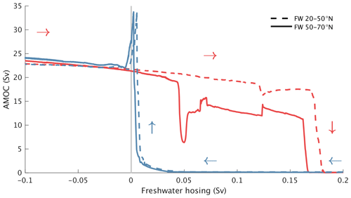
Figure 1Hysteresis of the AMOC in freshwater space. AMOC response to prescribed changes in FWF in two different latitudinal belts in the North Atlantic (dashed lines for 20–50° N and solid lines for 50–70° N). The red lines are from simulations with increasing FWF starting at −0.5 Sv, and the blue lines are for experiments with decreasing FWF starting at +0.5 Sv. In all cases the rate of change of the imposed FWF is 0.02 Sv kyr−1, meaning that each full simulation covering the FWF range between −0.5 Sv to +0.5 Sv (only partly shown in the figure) corresponds to 50 000 simulation years. The AMOC strength is defined as the maximum of the Atlantic meridional streamfunction deeper than 700 m.
In our freshwater hysteresis experiments in Fig. 1 we applied a very slow rate of change of 0.02 Sv per 1000 years in the FWF. When repeating the experiment with a 10-times-higher rate of change (0.2 Sv kyr−1), a value typically used in computationally expensive state-of-the-art climate models (e.g. Hu et al., 2012; van Westen and Dijkstra, 2023), the hysteresis looks very different (Fig. B2). For a higher rate of change in the forcing, the hysteresis is generally smoother and more regular and does not show the abrupt transitions that characterize the hysteresis curves produced with slow FWF changes. Notably, the Weak AMOC mode is not captured in the fast hysteresis experiments, where the AMOC is gradually transitioning to an Off state when the FWF exceeds ∼ 0.05 Sv (Fig. B2b). In the experiments with decreasing FWF, a higher forcing rate leads to a much delayed recovery of the AMOC from the Off state, resulting in a very distorted representation of the bistability range. In particular, the slow forcing experiments show that the AMOC is monostable under pre-industrial conditions in our model, while the fast forcing simulations give the wrong impression that the AMOC Off state is also stable (Fig. B2).
Another way of looking at AMOC stability is to investigate the AMOC response to changes in atmospheric CO2. In Fig. 2 the CO2 concentration is very slowly increased starting from 180 ppm up to 560 ppm (0.002 % yr−1; see also Appendix A2). The model shows a general increase in AMOC strength with increasing global temperature under quasi-equilibrium conditions (Fig. 2, red line). A weaker AMOC for CO2 concentrations lower than pre-industrial values has also been found in general circulation models (Stouffer and Manabe, 2003; Oka et al., 2012, 2021; Brown and Galbraith, 2016; Klockmann et al., 2018; Galbraith and de Lavergne, 2019). Stouffer and Manabe (2003) found AMOC strengthening under doubling and quadrupling of CO2 relative to pre-industrial levels, and recently Bonan et al. (2022) showed that at least some state-of-the-art climate models produce an AMOC that is appreciably stronger under CO2 quadrupling. Gérard and Crucifix (2024) recently analysed the AMOC response to a slow CO2 increase and found a gradual AMOC weakening and eventual collapse at CO2 above ∼ 1500 ppm. This is in contrast to our results, which show an increase in AMOC strength with increasing CO2, at least up to a CO2 concentration of 560 ppm. It should be noted that in both Gérard and Crucifix (2024) and our study the CO2 increase is slow enough to track the equilibrium AMOC response.
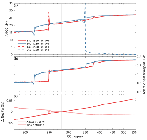
Figure 2Quasi-equilibrium AMOC response to changes in CO2. (a) Maximum of the AMOC streamfunction deeper than 700 m, (b) maximum meridional heat transport by the ocean in the Atlantic and (c) changes in net surface freshwater flux in the Atlantic (dark red line for the area > 50° N and light red line for the whole Atlantic ocean) in simulations with slowly varying prescribed atmospheric CO2 concentrations for CO2 increasing from 180 ppm (red lines) and for CO2 decreasing from 560 ppm (blue lines). The solid lines are from simulations initialized from a pre-industrial AMOC state, while the dashed lines are from simulations initialized from the AMOC Off state. In panels (b) and (c) only selected simulations are shown. The solid vertical line indicates the pre-industrial CO2 concentration of 280 ppm.
The general AMOC strengthening with warming in the model is punctuated by two abrupt transitions at ∼ 250 and ∼ 370 ppm (Fig. 2), separating three different AMOC states and convection patterns in the North Atlantic (Fig. 3). The different AMOC states are formally defined based on a critical depth of the maximum mixed-layer depth in three different regions in the northern North Atlantic as shown in Fig. B3. A stronger AMOC is generally associated with a northward shift in the sites of deepwater formation (Fig. 3f–h), following the northward retreat of sea ice (Fig. 3b–d). A few general circulation models found thermal AMOC thresholds under climate conditions generally colder than the pre-industrial, leading to abrupt AMOC weakening when climate is cooled and abrupt AMOC strengthening when climate is warmed (Knorr and Lohmann, 2007; Banderas et al., 2012; Oka et al., 2012; Zhang et al., 2017). Adloff et al. (2024) also found several thermal thresholds in the AMOC in idealized simulations of the last glacial cycle.
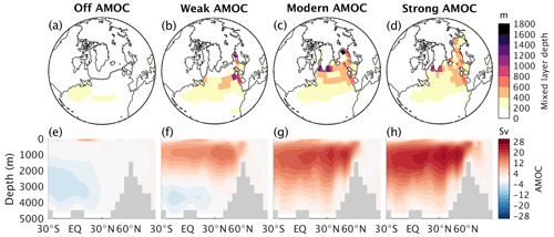
Figure 3The different AMOC states. (a–d) Maximum monthly mean mixed-layer depth of the year and (e–h) AMOC streamfunction for the different equilibrium AMOC states in the model: (a, e) Off, (b, f) Weak, (c, g) Modern and (d, h) Strong AMOC states. The grey line in (a)–(d) shows the maximum monthly mean sea ice extent of the year (defined as sea ice concentration > 0.15). The shown AMOC states are all for the same boundary conditions of 400 ppm of atmospheric CO2 and a FWF of +0.05 Sv, i.e. for the boundary conditions under which all four AMOC states co-exist in the model (Fig. 5).
Willeit et al. (2024) have shown that around the transition between a Modern and Weak AMOC at ∼ 250 ppm CLIMBER-X simulates Dansgaard–Oeschger-like events in the presence of noise, even with modern ice sheets. This millennial-scale variability originates from internal climate system dynamics associated with transitions between two distinct convection patterns that are stable for different CO2 concentrations. For CO2 above ∼ 250 ppm, the convection pattern resembles the present-day state, with deep water forming in the Labrador Sea and in the Nordic Seas (Fig. 3c), while for CO2 below ∼ 250 ppm convection cannot be sustained in the Labrador and Irminger seas and is generally restricted to areas south of ∼ 55° N (Fig. 3b). This state is equivalent to the Weak AMOC state in Fig. 1. A narrow window of CO2 concentrations exists for which both convection patterns are stable for the same CO2 (Fig. 2, solid red vs. solid blue lines), but in Willeit et al. (2024) it was shown that this bistability is not a requirement for the existence of millennial-scale variability, for which it is sufficient that the system is close enough to the bifurcation point between Modern and Weak AMOC states. It should be noted that in the past CO2 concentrations below the pre-industrial level of 280 ppm were related to the appearance of continental ice sheets over the NH, which affect AMOC stability (e.g. Zhang et al., 2014; Klockmann et al., 2018; Willeit et al., 2024) but are not considered in the present study.
The AMOC transition at ∼ 370 ppm is associated with a convection start in the Kara Sea and Nansen Basin (Fig. 3c) and has a clearer imprint in the Atlantic meridional heat transport (Fig. 2b) than in the maximum strength of the AMOC (Fig. 2a). We term this the “Strong” AMOC state. Convection in the Arctic is triggered in several climate models in response to future transient global warming (Brodeau and Koenigk, 2016; Lique et al., 2018; Lique and Thomas, 2018; Bretones et al., 2022; Pan et al., 2023), although in many other models this does not occur (Heuzé and Liu, 2024). However, the fact that convection in the Arctic in some models starts even in transient simulations that are characterized by an overall weakening of the AMOC suggests that the Arctic would be a plausible new location of deep-water formation in a warmer climate under quasi-equilibrium conditions.
Model simulations initialized at 180 ppm with an Off AMOC state (see Appendix A2) (Fig. 2a, dashed red line) indicate that the AMOC Off state is not stable for CO2 concentrations below pre-industrial levels, resulting in a monostable AMOC for pre-industrial conditions in our model (excluding the relatively narrow hysteresis around the transition between 220 and 250 ppm). However, if the model is initialized in an AMOC Off state at 560 ppm, the AMOC remains in the Off state as long as CO2 decreases to values below ∼ 350 ppm, after which the AMOC recovers with an overshoot (Fig. 2a, dashed blue line). Our model has therefore two widely different stable AMOC states for CO2 concentrations above ∼ 350 ppm, the AMOC Off state and a Strong state characterized by a more vigorous AMOC than Modern states (Fig. 2a). Hu et al. (2023) performed a similar AMOC hysteresis analysis using future climate scenarios and found that the AMOC exhibits two stable states for CO2 concentrations ∼ 1000 ppm in their model.
It is interesting to note that the AMOC strengthening with global warming occurs despite an associated increase in the net surface freshwater flux into the northern North Atlantic north of 50° N (Fig. 2c). This is a result of an intensification of the hydrological cycle in a warming climate, with the typical wet-gets-wetter and dry-gets-drier pattern (Held and Soden, 2006; Zhang et al., 2013). For double the amount of CO2, the net freshwater flux into the northern North Atlantic increases by ∼ 0.07 Sv, a relatively large freshwater flux, which is approximately an order of magnitude higher than the net freshwater flux from the Greenland ice sheet simulated under similar temperatures (e.g. Calov et al., 2018; Briner et al., 2020) and would roughly correspond to the rate of freshwater input resulting from the Greenland ice sheet melting completely over a time period of ∼ 1500 years. The increase in freshwater at high latitudes in the Atlantic as a response to global warming is also a consistent feature of CMIP6 models under transient future scenarios (Fig. B4a). While the northern North Atlantic gets wetter as climate warms, the net surface freshwater flux into the whole Atlantic Ocean shows the opposite trend in our model, with a small decrease in net freshwater flux as CO2 concentrations increase (Fig. 2c). Most CMIP6 models show a larger decrease in the net freshwater flux into the Atlantic than CLIMBER-X as climate warms (Fig. B4b) but with a relatively widespread between models.
The effect of changes in the net surface freshwater flux associated with global warming on AMOC stability is therefore the result of two competing effects: (i) salinification of the Atlantic as a whole, which stabilizes the AMOC through the salt–advection feedback, and (ii) the freshening of the northern Atlantic region, which destabilizes the AMOC through an increased surface buoyancy flux and a consequent lowering of the surface seawater density in the deep-water formation regions.
The above analyses of the response of the AMOC to changes in FWF and atmospheric CO2 have shown that there are at least four different stable AMOC states in CLIMBER-X, namely Off, Weak, Modern and Strong. The CO2–freshwater conditions under which these different AMOC states are stable can be investigated by tracing the AMOC response in the CO2–FWF space. This is done by slowly following the CO2–FWF paths illustrated in Fig. A2 as described in detail in Appendix A2. The standard approach to tracing the AMOC stability diagram is to slowly change one of the control parameters (usually FWF) first in one direction and then in the opposite direction. However, such a method often fails to trace all equilibria, especially when more than two equilibrium states coexist at the same point in the phase space. Therefore, we combined the traditional approach, which works in our case for the Strong and Off modes, with a more sophisticated procedure where we alternate changes in FWF and CO2 space to trace the Modern and Weak states (Fig. A2). The results are shown separately for each AMOC state in Fig. 4. High CO2 and low FWF generally favour stronger AMOC states (Figs. 4 and 5). The Strong AMOC state is characteristic of climates warmer than pre-industrial conditions (Fig. 4d). As seen already in Fig. 2, without FWF the AMOC transitions to the Strong state for CO2 concentrations above ∼ 380 ppm. The Modern AMOC state covers conditions going from low CO2 and negative FWF to high CO2 and FWF up to 0.1 Sv, passing through pre-industrial conditions (Fig. 4c). If the climate would be in equilibrium with present-day CO2 concentrations of ∼420 ppm, the model suggests that the Modern AMOC state would not be stable and that the AMOC would instead be in the Strong state (Fig. 4c, d). The Weak AMOC state exists for a range of CO2 concentrations between ∼ 200 and ∼ 560 ppm and FWF roughly between −0.05 and 0.18 Sv (Fig. 4b). Starting from pre-industrial conditions the Weak AMOC state can be reached either by reducing CO2 or by adding freshwater into the North Atlantic north of 50° N, as shown also in Fig. 2a and b and Fig. 1. For the investigated range of CO2 concentrations, an Off AMOC state cannot be achieved by varying CO2 alone and can only be reached through a large enough FWF. Under quasi-equilibrium conditions, the FWF needed to shut down the AMOC when starting from an On AMOC state is in the range ∼ 0.05–0.2 Sv, depending on the CO2 concentration (Fig. 4b and Fig. 5). If the FWF is larger than ∼0.05 Sv, the Off AMOC state is stable for any CO2 concentration (Fig. 4a). For smaller or negative FWF the stability of the Off state depends on CO2. The AMOC bistability range generally broadens with warming (Fig. 5), particularly because the AMOC recovery from the Off state requires an increasingly more negative FWF (Fig. 4a). In the model, the Off state is not stable under pre-industrial conditions, but it is stable for higher CO2 concentrations (Fig. 4a).
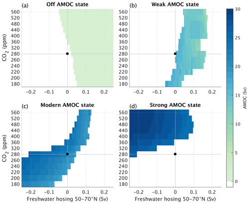
Figure 4AMOC states in combined CO2 and freshwater space. Maximum of the AMOC streamfunction as a function of CO2 and FWF between 50–70° N separately for the four different stable AMOC states in the model, namely (a) Off AMOC state, (b) Weak AMOC state, (c) Modern AMOC state and (d) Strong AMOC state. The different states are formally defined based on a critical threshold (mld m) of the maximum mixed-layer depth (mldmax) in three separate regions in the North Atlantic, namely (i) the Nordic Seas, (ii) the Labrador Sea, and (iii) the Barents and Kara seas and the Nansen Basin. Off is given by mldmax< mld in (i)–(iii), Weak is given by mldmax> mld in (i) and mldmax< mld in (ii)–(iii), Modern is given by mldmax> mld in (i)–(ii) and mldmax< mld in (iii), and Strong is given by mldmax> mld in (i)–(iii). The black dot indicates pre-industrial conditions. The stability landscape is constructed based on simulations following the paths shown in Fig. A2, where the rate of change of CO2 is 0.002 % yr−1 as in Fig. 2 and the rate of change of FWF is 0.02 Sv kyr−1 as in Fig. 1.
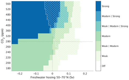
Figure 5Summary of AMOC stability landscape in combined CO2 and freshwater space. The coloured regions indicate the On AMOC states that are stable under the given CO2 and FWF as indicated in the legend. The filled white area indicates where only the Off AMOC state is stable, while the hatched white area shows the domain where the Off AMOC state and one or more of the three On AMOC states coexist. Note that multiple AMOC states are stable under some boundary conditions.
We use the remarkable fact that all four AMOC states in the model are stable under the same boundary conditions for CO2 concentrations ∼ 440 ppm and FWF ∼ 0.05 Sv (Fig. 5) to isolate the effect of the changes in AMOC states on the climate. An AMOC weakening generally causes a cooling that is most pronounced in the northern North Atlantic but that also extends more widely to the middle to high latitudes of the Northern Hemisphere (Fig. 6), with the largest effect being observed in winter (Fig. 6e–h) and the weakest in summer (Fig. 6i–l). This is in general agreement with previous studies looking at the climate impact of an AMOC shutdown forced by FWF (e.g. Jackson et al., 2015; van Westen and Dijkstra, 2023). The largest possible effect of AMOC on climate is for a transition between the Strong and Off states (Fig. 6a, e, i), which shows an annual mean cooling of up to 20 °C in the northern North Atlantic, with temperatures as much as ∼ 25–30 °C colder in winter and also associated with a pronounced sea ice advance (Fig. 6e). A shift from Strong to Modern AMOC induces a cooling of ∼ 10 °C in the Barents and Kara seas (Fig. 6b, f, j). A slow increase in the CO2 concentration, which would trigger a Modern to Strong AMOC transition as shown in Fig. 2a, would therefore cause a warming in these regions, with the opposite sign of changes in Fig. 6b, f and j. A transition from Modern to Weak AMOC mainly affects the Nordic Seas with a cooling by up to ∼ 15 °C in winter (Fig. 6c, g, k). A shift from a Weak to an Off AMOC state has a strong imprint on temperatures in the Nordic Seas and the Labrador and Irminger seas (Fig. 6d, h, l). In general, the differences in climate between the different AMOC states are related to changes in ocean heat transport, the shifts in the location of deep-water formation in the North Atlantic and the associated changes in sea ice extent (Fig. 3a–d). While the temperature differences in Fig. 6 are representative of the impact of the different AMOC states on climate, they are strictly valid only for an atmospheric CO2 of 400 ppm and a freshwater forcing of 0.05 Sv and could differ if the transition between AMOC states occurs under different boundary conditions.
For the first time, we have performed a systematic analysis of the AMOC stability in the FWF–CO2 space. This was done by very slowly varying the surface freshwater flux in the North Atlantic and the atmospheric CO2 concentration and required ∼ 1 000 000 model years of simulation.
We found four distinct modes of the AMOC. Apart from an Off AMOC state with no North Atlantic deep-water formation and a Modern-like AMOC state with deep water forming in the Labrador Sea and Nordic Seas as observed at present, we find two additional equilibrium states: (i) a Weak, stadial-like, AMOC state with deep water forming predominantly south of ∼ 55° N and (ii) a Strong AMOC state with convection reaching into the Arctic. Intermediate stable AMOC states between Modern and Off associated with changes in the convection pattern have also been found in previous studies (Rahmstorf, 1995; Lohmann et al., 2024) using ocean-only models forced with increasing FWF, but our results indicate that the standard method of tracing hysteresis in the FWF space may not be enough to find all possible AMOC modes.
Our AMOC stability landscape demonstrates that interglacial climates of the Quaternary are generally stable because of the mono-stability of the AMOC under pre-industrial-like conditions. The fact that the AMOC is monostable for CO2 concentrations around 280 ppm, a typical value for interglacials, in the absence of FWF also explains why the AMOC always recovered at the end of glacial terminations after temporary shutdowns induced by the freshwater input (∼ 0.1 Sv) from rapidly melting ice sheets. The existence of the Weak AMOC state has been shown by Willeit et al. (2024) to be related to Dansgaard–Oeschger events in the model, explaining the large AMOC variability observed during glacial times. Our results suggest that a different mode of AMOC (the Strong state) was possible during past warm climate conditions. The Pliocene was the most recent period in Earth's history with elevated atmospheric CO2 concentrations of ∼ 400 ppm (Martínez-Botí et al., 2015; Seki et al., 2010), which, according to our results, would be high enough to push the AMOC to a Strong state. There is indeed proxy-based evidence of a stronger-than-present AMOC in the Pliocene (Raymo et al., 1996; Ravelo and Andreasen, 2000) with an increased northward ocean heat transport in the Atlantic (Dowsett et al., 1992), which is consistent with sea surface temperature reconstructions for this period showing warmer conditions in the North Atlantic (McClymont et al., 2020). Climate models also tend to produce a stronger AMOC under mid-Pliocene conditions, albeit with considerable spread (Zhang et al., 2021; Weiffenbach et al., 2023). Whether the existence of the Strong AMOC state could potentially lead to some kind of centennial- or millennial-scale variability in the AMOC in a warmer climate remains to be explored.
As long as freshwater input from melting ice sheets is small, our results indicate a generally stronger and deeper AMOC at equilibrium under warmer climate conditions. This does not contradict the projected AMOC weakening response to anthropogenic global warming (e.g. Bellomo et al., 2021; Weijer et al., 2020; Weaver et al., 2012), which is an intrinsically transient response of the system predominantly induced by the rapid temperature increase (Gregory et al., 2005; Weaver et al., 2007; Levang and Schmitt, 2020). For present-day conditions and even up to the highest considered CO2 concentration of 560 ppm, the net freshwater flux from Greenland is small (≪ 0.1 Sv; Otosaka et al., 2023; Calov et al., 2018; Briner et al., 2020) and has therefore little effect on the AMOC, as also indicated by coupled climate–ice sheet model simulations (Bakker et al., 2016; Ackermann et al., 2020).
In the phase space, a CO2 increase drives the AMOC towards a stronger state. This is because the AMOC response to CO2 is fundamentally different from the response to FWF. In the case of FWF, regardless of the rate of change, an increase in FWF weakens the AMOC. In the case of CO2, this is not true: a fast enough increase in CO2 weakens the AMOC (Stocker and Schmittner, 1997), while a very slow (quasi-equilibrium) increase strengthens it. Since the main cause of future AMOC weakening is the increase in CO2, the traditional FWF hysteresis analysis is of limited use for predicting the future AMOC evolution. The non-trivial relation between future projected AMOC evolution and the stability landscape will be the subject of future work.
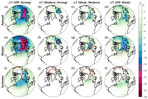
Figure 6Temperature differences induced by different AMOC states. (a–d) Annual, (e–h) winter (December–January–February) and (i–l) summer (June–July–August) temperature differences between different AMOC states as indicated in the panels. The coloured lines show the maximum monthly mean sea ice extent of the year in (e)–(h) and the seasonal minimum sea ice extent in (i)–(l), with the grey line always corresponding to the stronger AMOC state and the orange line to the weaker AMOC state. Sea ice extent is defined as sea ice concentration > 0.15. The figure shows temperature differences between the different AMOC states for 400 ppm of atmospheric CO2 and a FWF of +0.05 Sv, i.e. for the boundary conditions under which all four AMOC states co-exist in the model (Fig. 5).
Even if our stability diagram cannot explain the AMOC response to transient CO2 forcing, it provides some information on whether the transient weakening of the AMOC is reversible (mono-stable regime) or irreversible (bi-stable). Our results suggest that a future AMOC shutdown, which could be triggered by the transient response to anthropogenic global warming, could be irreversible because the Off AMOC state is stable for CO2 concentrations above the present-day level. Our model simulations therefore indicate that in terms of stability landscape the AMOC is currently moving towards a stronger state but from a monostable into a bistable regime where the AMOC Off state is also stable. It is hence in principle possible that slightly different future global warming trajectories could lead in one case to an irreversible (on multi-centennial timescales) AMOC shutdown and in another case to a transient AMOC weakening followed by a transition into a Strong AMOC state, eventually resulting in fundamentally different climate conditions in the North Atlantic. Transient model simulations under future emission scenarios will have to be performed to explore this possibility.
It should be noted that the AMOC stability landscape presented above is a result of model simulations with the fast Earth system model CLIMBER-X, which has a relatively coarse resolution and whose ocean model is based on the quasi-geostrophic approximation, with all the attendant limitations. Generally, anything related to convection and changes in convective patterns is highly model dependent, with widely different results produced even among state-of-the-art general circulation models (Sgubin et al., 2017; Heuzé, 2017; Treguier et al., 2023). Obviously, this does not question the existence of distinct Stadial and Interstadial AMOC modes during glacial times. Since the experiments presented in the paper can only be performed with a model like CLIMBER-X, we believe that they are useful to illustrate the general concept of AMOC stability. CLIMBER-X does not produce internal interannual climate variability, and it is possible that different modes of the AMOC, which are distinct in our simulations, may not be distinguished in the presence of strong variability (e.g. Monahan, 2002). The presence of noise can also lead to spontaneous transitions between different AMOC modes, as demonstrated in Willeit et al. (2024). Intrinsic internal variability in general circulation models can make the tracing of the AMOC stability landscape problematic, and in this sense the absence of such variability in CLIMBER-X is actually an advantage of the model because it allows us to obtain the phase portrait of the system without noise and then simulate realistic dynamical behaviour of the system by adding the noise.
A1 Earth system model
We use the CLIMBER-X Earth system model (Willeit et al., 2022) in a climate-only setup, including the frictional–geostrophic 3D ocean model GOLDSTEIN (Edwards et al., 1998; Edwards and Marsh, 2005) with 23 vertical layers, the semi-empirical statistical–dynamical atmosphere model SESAM (Willeit et al., 2022), the dynamic–thermodynamic sea ice model SISIM (Willeit et al., 2022) and the land surface model with interactive vegetation PALADYN (Willeit and Ganopolski, 2016). All components of the climate model have a horizontal resolution of 5°×5°. Ice sheets are prescribed at their modern state, and the net FWF from ice sheets is zero. The model is open source, is described in detail in Willeit et al. (2022), and in general shows performances that are comparable with state-of-the-art CMIP6 models under different forcings and boundary conditions. In particular, the simulated present-day AMOC overturning profile at 26° N in the Atlantic is close to observations (Fig. A1), although it reaches levels that are a bit too deep. The present-day deep-convection patterns compare well to ocean reanalysis in the North Atlantic (Fig. 13 in Willeit et al., 2022).
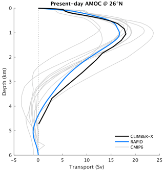
Figure A1Vertical profile of the simulated Atlantic meridional overturning streamfunction at 26° N (black) compared to observations from the RAPID array (Frajka-Williams et al., 2019) (blue) and a selection of CMIP6 models (grey). The CLIMBER-X and CMIP6 streamfunction is computed from historical simulations as the average over the time period from 2000–2014, while the RAPID values represent an average from 2004–2020.
A2 Experiments
With CLIMBER-X we ran transient simulations where we slowly varied either the FWF in the North Atlantic or the atmospheric CO2 concentration.
The standard FWF experiments were performed with prescribed changes in freshwater flux with a rate of ± 0.02 Sv kyr−1 in two different latitudinal belts, 20–50 and 50–70° N, in the North Atlantic, either starting from an initial hosing flux of −0.5 Sv and slowly increasing it until 0.5 Sv or starting from +0.5 Sv hosing flux and gradually decreasing it until −0.5 Sv. Each simulation is 50 000 years long. These two experiments were performed with prescribed constant CO2 concentration of 280 ppm. The initial condition for both these experiments is a pre-industrial equilibrium simulation run for 10 000 years with 280 ppm of CO2 and present-day ice sheets. To investigate how the rate of change of the FWF affects the hysteresis behaviour, we also repeated the freshwater hysteresis analysis using a 10× faster rate of change for the FWF (0.2 Sv kyr−1) and a slower rate of change of 0.005 Sv kyr−1).
We additionally performed transient simulations with slowly varying CO2 concentrations (i) starting at 180 ppm and gradually increasing CO2 up to 560 ppm and (ii) starting from 560 ppm and gradually decreasing CO2 down to 180 ppm. In both cases the rate of change of CO2 is 2 % kyr−1, implying a total simulation length of ∼ 56 500 years. We have chosen an exponential CO2 change rate in order to get a roughly linear global temperature response with time, considering the logarithmic dependence of the CO2 radiative forcing. The initial state for these simulations is a 10 000-year equilibrium run with either 180 ppm (for i) or 560 ppm (for ii) of atmospheric CO2. Simulations (i) and (ii) are also repeated using initial states where the AMOC is forced to be in the Off state. The 180 ppm and 560 ppm initial states with AMOC Off are obtained by prescribing 0.2 Sv of FWF in the latitudinal belt 50–70° N in the North Atlantic and running the model for 5000 years.
To investigate the stability of the four different AMOC states found from the FWF and CO2 perturbation experiments above in a combined FWF–CO2 space, we interactively designed simulation pathways through this parameter space, as shown in Fig. A2. The rate of change of the forcing in these experiments is again 0.02 Sv kyr−1 for FWF and 2 % kyr−1 for CO2. The constant CO2 concentrations used to move in the FWF direction are discretized in steps of 20 ppm between 180 and 280 ppm and in steps of 40 ppm between 280 and 560 ppm. The first step was to run experiments with increasing and decreasing FWF, starting from −0.5 Sv and +0.5 Sv, respectively, for all CO2 levels. These simulations are sufficient to trace the stability of the Off and Strong AMOC states (Fig. A2a, d) because (i) for large positive FWF the AMOC collapses under any CO2 concentration and (ii) for large negative FWF the AMOC always transitions to the Strong state. The stability analysis of the Modern and Weak AMOC states uses the pre-industrial state (CO2 of 280 ppm and zero FWF) as the initial condition but then requires a more sophisticated procedure to trace their stability through the 2D phase space (Fig. A2b, c).

Figure A2Simulation pathways used to explore the stability of the four different AMOC states in the combined CO2 and freshwater space plotted on top of the AMOC stability landscape shown in Fig. 4. The stability of the Off AMOC state in (a) was explored with simulations starting from a large FWF of +0.5 Sv and then gradually decreasing the FWF until the AMOC recovers for all levels of CO2. The stability of the Strong AMOC state in (d) was tracked in simulations starting from a large negative FWF of −0.5 Sv and then gradually increasing the FWF. For the investigation of the stability of the (b) Weak and (c) Modern AMOC states, the starting point was pre-industrial conditions, marked by the black dot. The black arrows indicate the primary path through the CO2 and FWF space, from which subsequent experiments with varying FWF in different directions are initialized (green arrows). Since the Strong AMOC state is not stable for CO2 lower than 280 ppm for the FWF range shown in the figure, the stability of the Modern AMOC state in (c) for CO2 lower than pre-industrial conditions is diagnosed from simulations initialized with a large negative FWF of −0.5 Sv, similar to what done in (d) for the Strong AMOC state. The rate of change of the forcing in all the experiments is 0.02 Sv kyr−1 for FWF and 2 % kyr−1 for CO2.
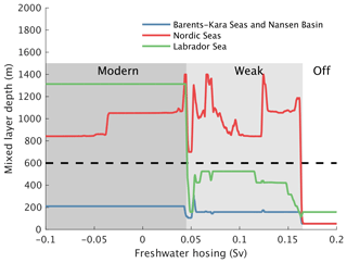
Figure B1Maximum mixed-layer depth in the three regions of the North Atlantic that are used to formally categorize the different AMOC states for the experiment with increasing freshwater hosing in the latitudinal belt between 50 and 70° N, corresponding to the solid red curve in Fig. 1. The dashed black line indicates the critical mixed-layer depth of 600 m used to discriminate between different convection patterns and AMOC states.
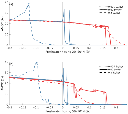
Figure B2Rate dependence of the hysteresis of the AMOC in freshwater space. AMOC response to prescribed changes in FWF in the latitudinal belts (a) 20–50° N and (b) 50–70° N. The red lines are from simulations with increasing FWF starting at −0.5 Sv, and the blue lines are for experiments with decreasing FWF starting at +0.5 Sv. The continuous lines are with the reference rate of change of the imposed FWF of 0.02 Sv kyr−1 as also shown in Fig. 1, the dashed lines represent simulations with a 10-fold increase in the rate of change of hosing (0.2 Sv kyr−1) and the dotted lines are for simulations with an even slower rate of change of 0.005 Sv kyr−1.
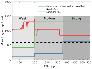
Figure B3Maximum mixed-layer depth in the three regions of the North Atlantic that are used to formally categorize the different AMOC states for the experiment with increasing CO2, corresponding to the solid red curve in Fig. 2. The dashed black line indicates the critical mixed-layer depth of 600 m used to discriminate between different convection patterns and AMOC states.
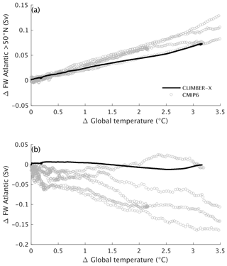
Figure B4Change in the net freshwater flux into the ocean as a function of global temperature change in transient historical and future simulations under the SSP2-4.5 scenario until the year 2300 CE for (a) the northern North Atlantic and Arctic (north of 50° N) and (b) the whole Atlantic Ocean. The solid line is for CLIMBER-X results, and the circles represent CMIP6 model results.
The CLIMBER-X model is freely available as open-source code at https://github.com/cxesmc/climber-x, last access: 30 August 2024.
MW and AG conceived and designed the study. MW performed the model simulations and created the figures. MW and AG wrote the paper.
The contact author has declared that neither of the authors has any competing interests.
Publisher’s note: Copernicus Publications remains neutral with regard to jurisdictional claims made in the text, published maps, institutional affiliations, or any other geographical representation in this paper. While Copernicus Publications makes every effort to include appropriate place names, the final responsibility lies with the authors.
The authors gratefully acknowledge the European Regional Development Fund (ERDF), the German Federal Ministry of Education and Research, and Land Brandenburg for supporting this project by providing resources on the high-performance computer system at the Potsdam Institute for Climate Impact Research. We would like to thank Yvan Romé and two anonymous reviewers for their valuable comments, which allowed us to substantially improve the manuscript.
This research has been supported by the Bundesministerium für Bildung und Forschung (grant no. PalMod 01LP1920B, 01LP1917D, 01LP2305B).
The publication of this article was funded by the Open Access Fund of the Leibniz Association.
This paper was edited by Christian Franzke and reviewed by Yvan Romé and two anonymous referees.
Ackermann, L., Danek, C., Gierz, P., and Lohmann, G.: AMOC Recovery in a Multicentennial Scenario Using a Coupled Atmosphere-Ocean-Ice Sheet Model, Geophys. Res. Lett., 47, e2019GL086810, https://doi.org/10.1029/2019GL086810, 2020. a
Adloff, M., Pöppelmeier, F., Jeltsch-Thömmes, A., Stocker, T. F., and Joos, F.: Multiple thermal Atlantic Meridional Overturning Circulation thresholds in the intermediate complexity model Bern3D, Clim. Past, 20, 1233–1250, https://doi.org/10.5194/cp-20-1233-2024, 2024. a
Ando, T. and Oka, A.: Hysteresis of the Glacial Atlantic Meridional Overturning Circulation Controlled by Thermal Feedbacks, Geophys. Res. Lett., 48, 1–9, https://doi.org/10.1029/2021GL095809, 2021. a, b, c
Bakker, P., Schmittner, A., Lenaerts, J. T., Abe-Ouchi, A., Bi, D., van den Broeke, M. R., Chan, W. L., Hu, A., Beadling, R. L., Marsland, S. J., Mernild, S. H., Saenko, O. A., Swingedouw, D., Sullivan, A., and Yin, J.: Fate of the Atlantic Meridional Overturning Circulation: Strong decline under continued warming and Greenland melting, Geophys. Res. Lett., 43, 12252–12260, https://doi.org/10.1002/2016GL070457, 2016. a
Banderas, R., Álvarez-Solas, J., and Montoya, M.: Role of CO2 and Southern Ocean winds in glacial abrupt climate change, Clim. Past, 8, 1011–1021, https://doi.org/10.5194/cp-8-1011-2012, 2012. a
Bellomo, K., Angeloni, M., Corti, S., and von Hardenberg, J.: Future climate change shaped by inter-model differences in Atlantic meridional overturning circulation response, Nat. Commun., 12, 1–10, https://doi.org/10.1038/s41467-021-24015-w, 2021. a, b
Bonan, D. B., Thompson, A. F., Newsom, E. R., Sun, S., and Rugenstein, M.: Transient and Equilibrium Responses of the Atlantic Overturning Circulation to Warming in Coupled Climate Models: The Role of Temperature and Salinity, J. Clim., 35, 5173–5193, https://doi.org/10.1175/JCLI-D-21-0912.1, 2022. a
Bretones, A., Nisancioglu, K. H., Jensen, M. F., Brakstad, A., and Yang, S.: Transient Increase in Arctic Deep-Water Formation and Ocean Circulation under Sea Ice Retreat, J. Clim., 35, 109–124, https://doi.org/10.1175/JCLI-D-21-0152.1, 2022. a
Briner, J. P., Cuzzone, J. K., Badgeley, J. A., Young, N. E., Steig, E. J., Morlighem, M., Schlegel, N. J., Hakim, G. J., Schaefer, J. M., Johnson, J. V., Lesnek, A. J., Thomas, E. K., Allan, E., Bennike, O., Cluett, A. A., Csatho, B., de Vernal, A., Downs, J., Larour, E., and Nowicki, S.: Rate of mass loss from the Greenland Ice Sheet will exceed Holocene values this century, Nature, 586, 70–74, https://doi.org/10.1038/s41586-020-2742-6, 2020. a, b
Brodeau, L. and Koenigk, T.: Extinction of the northern oceanic deep convection in an ensemble of climate model simulations of the 20th and 21st centuries, Clim. Dynam., 46, 2863–2882, https://doi.org/10.1007/s00382-015-2736-5, 2016. a
Brown, N. and Galbraith, E. D.: Hosed vs. unhosed: Interruptions of the Atlantic Meridional Overturning Circulation in a global coupled model, with and without freshwater forcing, Clim. Past, 12, 1663–1679, https://doi.org/10.5194/cp-12-1663-2016, 2016. a, b
Calov, R., Beyer, S., Greve, R., Beckmann, J., Willeit, M., Kleiner, T., Rückamp, M., Humbert, A., and Ganopolski, A.: Simulation of the future sea level contribution of Greenland with a new glacial system model, The Cryosphere, 12, 3097–3121, https://doi.org/10.5194/tc-12-3097-2018, 2018. a, b
Dowsett, H. J., Cronin, T. M., Poore, R. Z., Thompson, R. S., Whatley, R. C., and Wood, A. M.: Micropaleontological Evidence for Increased Meridional Heat Transport in the North Atlantic Ocean During the Pliocene, Science, 258, 1133–1135, https://doi.org/10.1126/science.258.5085.1133, 1992. a
Edwards, N. R. and Marsh, R.: Uncertainties due to transport-parameter sensitivity in an efficient 3-D ocean-climate model, Clim. Dynam., 24, 415–433, https://doi.org/10.1007/s00382-004-0508-8, 2005. a
Edwards, N. R., Willmott, A. J., and Killworth, P. D.: On the Role of Topography and Wind Stress on the Stability of the Thermohaline Circulation, J. Phys. Oceanogr., 28, 756–778, https://doi.org/10.1175/1520-0485(1998)028<0756:OTROTA>2.0.CO;2, 1998. a
Frajka-Williams, E., Ansorge, I. J., Baehr, J., Bryden, H. L., Chidichimo, M. P., Cunningham, S. A., Danabasoglu, G., Dong, S., Donohue, K. A., Elipot, S., Heimbach, P., Holliday, N. P., Hummels, R., Jackson, L. C., Karstensen, J., Lankhorst, M., Le Bras, I. A., Susan Lozier, M., McDonagh, E. L., Meinen, C. S., Mercier, H., Moat, B. I., Perez, R. C., Piecuch, C. G., Rhein, M., Srokosz, M. A., Trenberth, K. E., Bacon, S., Forget, G., Goni, G., Kieke, D., Koelling, J., Lamont, T., McCarthy, G. D., Mertens, C., Send, U., Smeed, D. A., Speich, S., van den Berg, M., Volkov, D., and Wilson, C.: Atlantic meridional overturning circulation: Observed transport and variability, Front. Mar. Sci., 6, 1–18, https://doi.org/10.3389/fmars.2019.00260, 2019. a
Galbraith, E. and de Lavergne, C.: Response of a comprehensive climate model to a broad range of external forcings: relevance for deep ocean ventilation and the development of late Cenozoic ice ages, Clim. Dynam., 52, 653–679, https://doi.org/10.1007/s00382-018-4157-8, 2019. a, b
Ganopolski, A. and Rahmstorf, S.: Rapid changes of glacial climate simulated in a coupled climate model, Nature, 409, 153–8, https://doi.org/10.1038/35051500, 2001. a, b, c, d
Gérard, J. and Crucifix, M.: Diagnosing the causes of AMOC slowdown in a coupled model: a cautionary tale, Earth Syst. Dynam., 15, 293–306, https://doi.org/10.5194/esd-15-293-2024, 2024. a, b, c, d
Gregory, J. M., Saenko, O. A., and Weaver, A. J.: The role of the Atlantic freshwater balance in the hysteresis of the meridional overturning circulation, Clim. Dynam., 21, 707–717, https://doi.org/10.1007/s00382-003-0359-8, 2003. a
Gregory, J. M., Dixon, K. W., Stouffer, R. J., Weaver, A. J., Driesschaert, E., Eby, M., Fichefet, T., Hasumi, H., Hu, A., Jungclaus, J. H., Kamenkovich, I. V., Levermann, A., Montoya, M., Murakami, S., Nawrath, S., Oka, A., Sokolov, A. P., and Thorpe, R. B.: A model intercomparison of changes in the Atlantic thermohaline circulation in response to increasing atmospheric CO2 concentration, Geophys. Res. Lett., 32, L12703, https://doi.org/10.1029/2005GL023209, 2005. a
Hawkins, E., Smith, R. S., Allison, L. C., Gregory, J. M., Woollings, T. J., Pohlmann, H., and De Cuevas, B.: Bistability of the Atlantic overturning circulation in a global climate model and links to ocean freshwater transport, Geophys. Res. Lett., 38, L10605, https://doi.org/10.1029/2011GL047208, 2011. a, b
Held, I. M. and Soden, B. J.: Robust Responses of the Hydrological Cycle to Global Warming, J. Clim., 19, 5686–5699, https://doi.org/10.1175/JCLI3990.1, 2006. a
Heuzé, C.: North Atlantic deep water formation and AMOC in CMIP5 models, Ocean Sci., 13, 609–622, https://doi.org/10.5194/os-13-609-2017, 2017. a
Heuzé, C. and Liu, H.: No Emergence of Deep Convection in the Arctic Ocean Across CMIP6 Models, Geophys. Res. Lett., 51, e2023GL106499, https://doi.org/10.1029/2023GL106499, 2024. a
Hofmann, M. and Rahmstorf, S.: On the stability of the Atlantic meridional overturning circulation, P. Natl. Acad. Sci. USA, 106, 20584–20589, https://doi.org/10.1073/pnas.0909146106, 2009. a, b
Hu, A., Meehl, G. A., Han, W., Timmermann, A., Otto-Bliesner, B., Liu, Z., Washington, W. M., Large, W., Abe-Ouchi, A., Kimoto, M., Lambeck, K., and Wu, B.: Role of the Bering Strait on the hysteresis of the ocean conveyor belt circulation and glacial climate stability, P. Natl. Acad. Sci. USA, 109, 6417–6422, https://doi.org/10.1073/pnas.1116014109, 2012. a, b, c, d
Hu, A., Meehl, G. A., Abe-Ouchi, A., Han, W., Otto-Bliesner, B., He, F., Wu, T., Rosenbloom, N., Strand, W. G., and Edwards, J.: Dichotomy between freshwater and heat flux effects on oceanic conveyor belt stability and global climate, Commun. Earth Environ., 4, 246, https://doi.org/10.1038/s43247-023-00916-0, 2023. a
Jackson, L. C. and Wood, R. A.: Hysteresis and Resilience of the AMOC in an Eddy-Permitting GCM, Geophys. Res. Lett., 45, 8547–8556, https://doi.org/10.1029/2018GL078104, 2018. a
Jackson, L. C., Kahana, R., Graham, T., Ringer, M. A., Woollings, T., Mecking, J. V., and Wood, R. A.: Global and European climate impacts of a slowdown of the AMOC in a high resolution GCM, Clim. Dynam., 45, 3299–3316, https://doi.org/10.1007/s00382-015-2540-2, 2015. a, b
Klockmann, M., Mikolajewicz, U., and Marotzke, J.: Two AMOC states in response to decreasing greenhouse gas concentrations in the coupled climate model MPI-ESM, J. Clim., 31, 7969–7984, https://doi.org/10.1175/JCLI-D-17-0859.1, 2018. a, b, c
Knorr, G. and Lohmann, G.: Rapid transitions in the Atlantic thermohaline circulation triggered by global warming and meltwater during the last deglaciation, Geochem. Geophy. Geosy., 8, Q12006, https://doi.org/10.1029/2007GC001604, 2007. a
Lenton, T. M., Myerscough, R. J., Marsh, R., Livina, V. N., Price, A. R., and Cox, S. J.: Using GENIE to study a tipping point in the climate system, Philos. T. R. Soc. A, 367, 871–884, https://doi.org/10.1098/rsta.2008.0171, 2009. a
Levang, S. J. and Schmitt, R. W.: What causes the AMOC to weaken in CMIP5?, J. Clim., 33, 1535–1545, https://doi.org/10.1175/JCLI-D-19-0547.1, 2020. a
Lique, C. and Thomas, M. D.: Latitudinal shift of the Atlantic Meridional Overturning Circulation source regions under a warming climate, Nat. Clim. Change, 8, 1013–1020, https://doi.org/10.1038/s41558-018-0316-5, 2018. a
Lique, C., Johnson, H. L., and Plancherel, Y.: Emergence of deep convection in the Arctic Ocean under a warming climate, Clim. Dynam., 50, 3833–3847, https://doi.org/10.1007/s00382-017-3849-9, 2018. a
Liu, W., Xie, S. P., Liu, Z., and Zhu, J.: Overlooked possibility of a collapsed atlantic meridional overturning circulation in warming climate, Sci. Adv., 3, e1601666, https://doi.org/10.1126/sciadv.1601666, 2017. a
Lohmann, J., Dijkstra, H. A., Jochum, M., Lucarini, V., and Ditlevsen, P. D.: Multistability and intermediate tipping of the Atlantic Ocean circulation, Sci. Adv., 10, eadi4253, https://doi.org/10.1126/sciadv.adi4253, 2024. a
Manabe, S. and Stouffer, R. J.: Two Stable Equilibria of a Coupled Ocean-Atmosphere Model, J. Clim., 6, 175–177, https://doi.org/10.1175/1520-0442(1993)006<0175:COSEOA>2.0.CO;2, 1988. a
Manabe, S. and Stouffer, R. J.: Century-scale effects of increased atmospheric CO2 on the ocean–atmosphere system, Nature, 364, 215–218, https://doi.org/10.1038/364215a0, 1993. a
Martínez-Botí, M. A., Foster, G. L., Chalk, T. B., Rohling, E. J., Sexton, P. F., Lunt, D. J., Pancost, R. D., Badger, M. P. S., and Schmidt, D. N.: Plio-Pleistocene climate sensitivity evaluated using high-resolution CO2 records, Nature, 518, 49–54, https://doi.org/10.1038/nature14145, 2015. a
McClymont, E. L., Ford, H. L., Ling Ho, S., Tindall, J. C., Haywood, A. M., Alonso-Garcia, M., Bailey, I., Berke, M. A., Littler, K., Patterson, M. O., Petrick, B., Peterse, F., Christina Ravelo, A., Risebrobakken, B., De Schepper, S., Swann, G. E., Thirumalai, K., Tierney, J. E., Van Der Weijst, C., White, S., Abe-Ouchi, A., Baatsen, M. L., Brady, E. C., Chan, W. L., Chandan, D., Feng, R., Guo, C., Von Der Heydt, A. S., Hunter, S., Li, X., Lohmann, G., Nisancioglu, K. H., Otto-Bliesner, B. L., Richard Peltier, W., Stepanek, C., and Zhang, Z.: Lessons from a high-CO2 world: An ocean view from ∼3 million years ago, Clim. Past, 16, 1599–1615, https://doi.org/10.5194/cp-16-1599-2020, 2020. a
Mecking, J. V., Drijfhout, S. S., Jackson, L. C., and Graham, T.: Stable AMOC off state in an eddy – permitting coupled climate model, Clim. Dynam., 47, 2455–2470, https://doi.org/10.1007/s00382-016-2975-0, 2016. a
Monahan, A. H.: Stabilization of climate regimes by noise in a simple model of the thermohaline circulation, J. Phys. Oceanogr., 32, 2072–2085, https://doi.org/10.1175/1520-0485(2002)032<2072:SOCRBN>2.0.CO;2, 2002. a
Oka, A., Hasumi, H., and Abe-Ouchi, A.: The thermal threshold of the Atlantic meridional overturning circulation and its control by wind stress forcing during glacial climate, Geophys. Res. Lett., 39, L09709, https://doi.org/10.1029/2012GL051421, 2012. a, b
Oka, A., Abe-Ouchi, A., Sherriff-Tadano, S., Yokoyama, Y., Kawamura, K., and Hasumi, H.: Glacial mode shift of the Atlantic meridional overturning circulation by warming over the Southern Ocean, Commun. Earth Environ., 2, 169, https://doi.org/10.1038/s43247-021-00226-3, 2021. a
Otosaka, I. N., Shepherd, A., Ivins, E. R., Schlegel, N. J., Amory, C., Van Den Broeke, M. R., Horwath, M., Joughin, I., King, M. D., Krinner, G., Nowicki, S., Payne, A. J., Rignot, E., Scambos, T., Simon, K. M., Smith, B. E., Sørensen, L. S., Velicogna, I., Whitehouse, P. L., Geruo, A., Agosta, C., Ahlstrøm, A. P., Blazquez, A., Colgan, W., Engdahl, M. E., Fettweis, X., Forsberg, R., Gallée, H., Gardner, A., Gilbert, L., Gourmelen, N., Groh, A., Gunter, B. C., Harig, C., Helm, V., Khan, S. A., Kittel, C., Konrad, H., Langen, P. L., Lecavalier, B. S., Liang, C. C., Loomis, B. D., McMillan, M., Melini, D., Mernild, S. H., Mottram, R., Mouginot, J., Nilsson, J., Noël, B., Pattle, M. E., Peltier, W. R., Pie, N., Roca, M., Sasgen, I., Save, H. V., Seo, K. W., Scheuchl, B., Schrama, E. J., Schröder, L., Simonsen, S. B., Slater, T., Spada, G., Sutterley, T. C., Vishwakarma, B. D., Van Wessem, J. M., Wiese, D., Van Der Wal, W., and Wouters, B.: Mass balance of the Greenland and Antarctic ice sheets from 1992 to 2020, Earth Syst. Sci. Data, 15, 1597–1616, https://doi.org/10.5194/essd-15-1597-2023, 2023. a
Pan, R., Shu, Q., Wang, Q., Wang, S., Song, Z., He, Y., and Qiao, F.: Future Arctic Climate Change in CMIP6 Strikingly Intensified by NEMO-Family Climate Models, Geophys. Res. Lett., 50, e2022GL102077, https://doi.org/10.1029/2022GL102077, 2023. a
Pöppelmeier, F., Scheen, J., Jeltsch-Thömmes, A., and F. Stocker, T.: Simulated stability of the Atlantic Meridional Overturning Circulation during the Last Glacial Maximum, Clim. Past, 17, 615–632, https://doi.org/10.5194/cp-17-615-2021, 2021. a
Prange, M., Romanova, V., and Lohmann, G.: The glacial thermohaline circulation: Stable or unstable?, Geophys. Res. Lett., 29, 24-1–24-4, https://doi.org/10.1029/2002GL015337, 2002. a
Rahmstorf, S.: Bifurcations of the Atlantic thermohaline circulation in response to changes in the hydrological cycle, Nature, 378, 145–149, https://doi.org/10.1038/378145a0, 1995. a, b, c
Rahmstorf, S., Crucifix, M., Ganopolski, A., Goosse, H., Kamenkovich, I., Knutti, R., Lohmann, G., Marsh, R., Mysak, L. A., Wang, Z., and Weaver, A. J.: Thermohaline circulation hysteresis: A model intercomparison, Geophys. Res. Lett., 32, L23605, https://doi.org/10.1029/2005GL023655, 2005. a, b, c, d
Ravelo, A. C. and Andreasen, D. H.: Enhanced circulation during a warm period, Geophys. Res. Lett., 27, 1001–1004, https://doi.org/10.1029/1999GL007000, 2000. a
Raymo, M., Grant, B., Horowitz, M., and Rau, G.: Mid-Pliocene warmth: stronger greenhouse and stronger conveyor, Mar. Micropaleontol., 27, 313–326, https://doi.org/10.1016/0377-8398(95)00048-8, 1996. a
Roquet, F., Madec, G., Brodeau, L., and Nycander, J.: Defining a simplified yet “Realistic” equation of state for seawater, J. Phys. Oceanogr., 45, 2564–2579, https://doi.org/10.1175/JPO-D-15-0080.1, 2015. a
Schmittner, A., Yoshimori, M., and Weaver, A. J.: Instability of glacial climate in a model of the ocean-atmosphere-cryosphere system, Science, 295, 1489–1493, https://doi.org/10.1126/science.1066174, 2002. a
Seki, O., Foster, G. L., Schmidt, D. N., Mackensen, A., Kawamura, K., and Pancost, R. D.: Alkenone and boron-based Pliocene pCO2 records, Earth Planet. Sc. Lett., 292, 201–211, https://doi.org/10.1016/j.epsl.2010.01.037, 2010. a
Sgubin, G., Swingedouw, D., Drijfhout, S., Mary, Y., and Bennabi, A.: Abrupt cooling over the North Atlantic in modern climate models, Nat. Commun., 8, 14375, https://doi.org/10.1038/ncomms14375, 2017. a
Smith, R. S. and Gregory, J. M.: A study of the sensitivity of ocean overturning circulation and climate to freshwater input in different regions of the North Atlantic, Geophys. Res. Lett., 36, L15701, https://doi.org/10.1029/2009GL038607, 2009. a
Stocker, T. F. and Schmittner, A.: Influence of CO2 emission rates on the stability of the thermohaline circulation, Nature, 388, 862–865, https://doi.org/10.1038/42224, 1997. a
Stocker, T. F. and Wright, D. G.: Rapid transitions of the ocean's deep circulation induced by changes in surface water fluxes, Nature, 351, 729–732, https://doi.org/10.1038/351729a0, 1991. a, b
Stommel, H.: Thermohaline Convection with Two Stable Regimes of Flow, Tellus, 13, 224–230, https://doi.org/10.1111/j.2153-3490.1961.tb00079.x, 1961. a, b
Stouffer, R. J. and Manabe, S.: Equilibrium response of thermohaline circulation to large changes in atmospheric CO2 concentration, Clim. Dynam., 20, 759–773, https://doi.org/10.1007/s00382-002-0302-4, 2003. a, b
Treguier, A. M., De Boyer Montégut, C., Bozec, A., Chassignet, E. P., Fox-Kemper, B., McC Hogg, A., Iovino, D., Kiss, A. E., Le Sommer, J., Li, Y., Lin, P., Lique, C., Liu, H., Serazin, G., Sidorenko, D., Wang, Q., Xu, X., and Yeager, S.: The mixed-layer depth in the Ocean Model Intercomparison Project (OMIP): impact of resolving mesoscale eddies, Geosci.Model Dev., 16, 3849–3872, https://doi.org/10.5194/gmd-16-3849-2023, 2023. a
van Westen, R. M. and Dijkstra, H. A.: Asymmetry of AMOC Hysteresis in a State-Of-The-Art Global Climate Model, Geophys. Res. Lett., 50, e2023GL106088, https://doi.org/10.1029/2023GL106088, 2023. a, b, c, d, e
Weaver, A. J., Eby, M., Kienast, M., and Saenko, O. A.: Response of the Atlantic meridional overturning circulation to increasing atmospheric CO2: Sensitivity to mean climate state, Geophys. Res. Lett., 34, L05708, https://doi.org/10.1029/2006GL028756, 2007. a
Weaver, A. J., Sedláček, J., Eby, M., Alexander, K., Crespin, E., Fichefet, T., Philippon-Berthier, G., Joos, F., Kawamiy, M., Matsumoto, K., Steinacher, M., Tachiiri, K., Tokos, K., Yoshimori, M., and Zickfeld, K.: Stability of the Atlantic meridional overturning circulation: A model intercomparison, Geophys. Res. Lett., 39, L20709, https://doi.org/10.1029/2012GL053763, 2012. a, b
Weber, S. L. and Drijthout, S. S.: Stability of the Atlantic Meridional Overturning Circulation in the last glacial maximum climate, Geophys. Res. Lett., 34, L22706, https://doi.org/10.1029/2007GL031437, 2007. a
Weiffenbach, J. E., Baatsen, M. L., Dijkstra, H. A., Von Der Heydt, A. S., Abe-Ouchi, A., Brady, E. C., Chan, W. L., Chandan, D., Chandler, M. A., Contoux, C., Feng, R., Guo, C., Han, Z., Haywood, A. M., Li, Q., Li, X., Lohmann, G., Lunt, D. J., Nisancioglu, K. H., Otto-Bliesner, B. L., Peltier, W. R., Ramstein, G., Sohl, L. E., Stepanek, C., Tan, N., Tindall, J. C., Williams, C. J., Zhang, Q., and Zhang, Z.: Unraveling the mechanisms and implications of a stronger mid-Pliocene Atlantic Meridional Overturning Circulation (AMOC) in PlioMIP2, Clim. Past, 19, 61–85, https://doi.org/10.5194/cp-19-61-2023, 2023. a
Weijer, W., Cheng, W., Drijfhout, S. S., Fedorov, A. V., Hu, A., Jackson, L. C., Liu, W., McDonagh, E. L., Mecking, J. V., and Zhang, J.: Stability of the Atlantic Meridional Overturning Circulation: A Review and Synthesis, J. Geophys. Res.-Ocean., 124, 5336–5375, https://doi.org/10.1029/2019JC015083, 2019. a
Weijer, W., Cheng, W., Garuba, O. A., Hu, A., and Nadiga, B. T.: CMIP6 Models Predict Significant 21st Century Decline of the Atlantic Meridional Overturning Circulation, Geophys. Res. Lett., 47, e2019GL086075, https://doi.org/10.1029/2019GL086075, 2020. a, b
Willeit, M. and Ganopolski, A.: PALADYN v1.0, a comprehensive land surface-vegetation-carbon cycle model of intermediate complexity, Geosci. Model Dev., 9, 3817–3857, https://doi.org/10.5194/gmd-9-3817-2016, 2016. a
Willeit, M., Ganopolski, A., Robinson, A., and Edwards, N. R.: The Earth system model CLIMBER-X v1.0 – Part 1: Climate model description and validation, Geosci. Model Dev., 15, 5905–5948, https://doi.org/10.5194/gmd-15-5905-2022, 2022. a, b, c, d, e, f, g
Willeit, M., Ganopolski, A., Edwards, N. R., and Rahmstorf, S.: Surface buoyancy control of millennial-scale variations of the Atlantic meridional ocean circulation, EGUsphere [preprint], https://doi.org/10.5194/egusphere-2024-819, 2024. a, b, c, d, e, f, g, h
Zhang, X., He, J., Zhang, J., Polyakov, I., Gerdes, R., Inoue, J., and Wu, P.: Enhanced poleward moisture transport and amplified northern high-latitude wetting trend, Nat. Clim. Change, 3, 47–51, https://doi.org/10.1038/nclimate1631, 2013. a
Zhang, X., Lohmann, G., Knorr, G., and Purcell, C.: Abrupt glacial climate shifts controlled by ice sheet changes, Nature, 512, 290–294, https://doi.org/10.1038/nature13592, 2014. a
Zhang, X., Knorr, G., Lohmann, G., and Barker, S.: Abrupt North Atlantic circulation changes in response to gradual CO2 forcing in a glacial climate state, Nat. Geosci., 10, 518–523, https://doi.org/10.1038/ngeo2974, 2017. a
Zhang, Z., Li, X., Guo, C., Helge Otterä, O., Nisancioglu, K. H., Tan, N., Contoux, C., Ramstein, G., Feng, R., Otto-Bliesner, B. L., Brady, E., Chandan, D., Richard Peltier, W., Baatsen, M. L., Von Der Heydt, A. S., Weiffenbach, J. E., Stepanek, C., Lohmann, G., Zhang, Q., Li, Q., Chandler, M. A., Sohl, L. E., Haywood, A. M., Hunter, S. J., Tindall, J. C., Williams, C., Lunt, D. J., Chan, W. L., and Abe-Ouchi, A.: Mid-Pliocene Atlantic Meridional Overturning Circulation simulated in PlioMIP2, Clim. Past, 17, 529–543, https://doi.org/10.5194/cp-17-529-2021, 2021. a
- Abstract
- Introduction
- AMOC hysteresis in freshwater space
- Equilibrium AMOC response to CO2 changes
- AMOC stability landscape in combined CO2 and freshwater space
- Discussion and conclusions
- Appendix A: Materials and methods
- Appendix B: Additional figures
- Code and data availability
- Author contributions
- Competing interests
- Disclaimer
- Acknowledgements
- Financial support
- Review statement
- References


