An enhanced Standardized Precipitation–Evapotranspiration Index (SPEI) drought-monitoring method integrating land surface characteristics

Atmospheric evaporative demand is a key metric for monitoring agricultural drought. Existing ways of estimating evaporative demand in drought indices do not faithfully represent the constraints imposed by land surface characteristics and become less accurate over nonuniform land surfaces. This study proposes incorporating surface vegetation characteristics, such as vegetation dynamics data, aerodynamic parameters, and physiological parameters, into existing potential-evapotranspiration (PET) methods. This approach is implemented across the continental United States (CONUS) for the period from 1981–2017 and is tested using a recently developed drought index, the Standardized Precipitation–Evapotranspiration Index (SPEI). We show that activating realistic maximum surface conductance and aerodynamic conductance could improve the prediction of soil moisture dynamics and drought impacts by 29 %–41 % on average compared to more simple, widely used methods. We also demonstrate that this is especially effective in forests and humid regions, with improvements of 86 %–89 %. Our approach only requires a minimal amount of ancillary data while allowing for both historical reconstruction and real-time drought forecasting. This offers a physically meaningful yet easy-to-implement way to account for vegetation control in drought indices.

1 Introduction

Drought is one of the most costly hydrological hazards (Wilhite, 2000; Ross and Lott, 2003; Piao et al., 2019), exhibiting devastating impacts on croplands and pastures (Kogan, 1995), forest ecosystems (Clark et al., 2016; Xu et al., 2022), electricity production, water quality, and soil fertility (Loon, 2015). Monitoring changes in water availability is critical for providing early warnings of drought and for risk management (Wilhite et al., 2014). Many physical and probabilistic measures have been developed (Heim, 2002) to quantify drought, such as the Palmer Drought Severity Index (PDSI; Palmer, 1965), the Standardized Precipitation Index (SPI; McKee et al., 1993), the Vegetation Condition Index (VCI; Kogan, 1995), and multiple remote sensing drought indices (Zhang et al., 2017; Yang et al., 2023).

Atmospheric evaporative demand (AED) is a key input for drought indices because it is a measure of water demand, i.e., how thirsty the atmosphere is (Peng et al., 2018). AED typically reflects the effects of temperature and humidity and is considered a major driver of drought stress on vegetation and tree mortality (Williams et al., 2012; McDowell et al., 2018). Among the many drought indices, the recently developed Standardized Precipitation–Evapotranspiration Index (SPEI) (Vicente-Serrano et al., 2010) incorporates water demand (AED) in addition to water supply (precipitation). Compared to the SPI, which only considers precipitation, the SPEI is more suitable for quantifying drought impacts on agriculture (Potop, 2011; Potop et al., 2012) and ecosystems (Vicente-Serrano et al., 2012, 2013; Barbeta et al., 2013). In addition, the SPEI is more flexible than the PDSI because it is not sensitive to soil water field capacity and can be implemented on various timescales (Vicente-Serrano et al., 2015; Zhao et al., 2017). It has been widely used for both drought reconstruction and monitoring (Paulo et al., 2012; Beguería et al., 2013).

The method used to estimate AED in drought indices has a significant impact on drought quantification (Sheffield et al., 2012; Trenberth et al., 2013; Yang et al., 2019; Dewes et al., 2017). AED is approximated by potential evapotranspiration (PET), which is the maximum rate of evapotranspiration when surface water supply is unlimited. Previous work has used various PET formulations for AED in the SPEI since the index was first proposed in 2010 (Vicente-Serrano et al., 2010; Beguería et al., 2013). These conventional PET methods do not factor in the effects of surface characteristics, which often assume no or simple universal vegetation controls on transpiration (e.g., the Thornthwaite, Hargreaves–Samani, and Penman methods). Without vegetation control, the maximum surface conductance is overestimated, and the PET rate during the onset and retreat of the growing season is unrealistically high. Furthermore, by assuming an smooth reference surface, some methods do not account for surface roughness, thereby downplaying aerodynamic conductance and suppressing the PET estimate (Peng et al., 2019). Although the reference evapotranspiration (ET₀) method (Allen et al., 1998) considers the biophysical limitations of transpiration by assigning a surface resistance under well-watered conditions, it does not account for vegetation phenology (Lorenz et al., 2013) and assumes a fixed reference height and constant surface resistance for all vegetation types. This approach is not physically meaningful for forests, where canopy height (CH) is relatively large and vegetation cover varies significantly. A recent study by Sun et al. (2023) highlighted the importance of incorporating surface properties, especially vegetation control, into PET methods and used a two-source Shuttleworth–Wallace (SW) model designed and validated for sparse and fragmented vegetation surfaces. However, without further calibration and parameterization, the SW model's broader applicability beyond sparse vegetation is uncertain, and, additionally, it may increase data requirements and associated uncertainties (Gao et al., 2021; Abeysiriwardana et al., 2022).

We hypothesize that adding surface vegetation characteristics to an existing drought quantification approach will improve the spatial and temporal accuracy of drought prediction. The goals of this study are to explore which surface features are the most useful for enhancing drought prediction and which vegetation types benefit most from incorporating these features. We propose incorporating realistic vegetation restrictions into existing PET methods while minimizing the cost and uncertainty caused by additional data sources and complex formulations. We then use independent soil moisture observations (Dai et al., 2004) from satellites to evaluate drought depictions using various forms of PET approaches across different temporal scales. The evaluation against observed soil moisture allows for the direct diagnosis of the most sensitive surface characteristics and the most effective approach for drought quantification (Vicente-Serrano et al., 2012).

In this study, we focus on the continental US (CONUS) primarily because drought events affecting this region have raised interest in the variability, trends, and future risks of drought (Andreadis and Lettenmaier, 2006; Hobbins et al., 2012; Dewes et al., 2017). Several severe droughts impacted the western US in the recent decade, including the 2012 Great Plains drought (Hoerling et al., 2014) and the 2012–2016 California drought (Dong et al., 2019). The western US has been experiencing its most severe drought period since the 1930s and 1950s (Andreadis et al., 2005), and its vulnerability to drought continues to grow (Andreadis and Lettenmaier, 2006). Additionally, high-quality meteorological datasets are available across the CONUS (Daly et al., 2008; Xia et al., 2012) and can help reduce the uncertainty in drought prediction originating from input forcings.

2 Data

2.1 Meteorology

To calculate the SPEI, PET is estimated on a daily scale over a period from 1981–2017 using high-quality daily meteorology data from the Parameter-elevation Regressions on Independent Slopes Model (PRISM), which employs weather stations and a digital elevation model (Daly et al., 1994, 2008). We acquire daily precipitation, as well as daily mean, maximum, minimum, and dew point temperatures, on a 4 km grid for the period from 1981–2017. Surface downward shortwave and net longwave radiation, pressure, and wind speed are taken from Phase 2 of the North American Land Data Assimilation System (NLDAS-2; Xia et al., 2012). All data are spatially restricted to the continental United States (25–50° N, 67–125° W) and regridded to the 0.125° NLDAS-2 grid using the first-order conservative remapping tool provided by the Climate Data Operators software (https://code.zmaw.de/projects/cdo, last access: 1 June 2017).

2.2 Soil moisture

Surface soil moisture (SMsurf) data from the European Space Agency Climate Change Initiative (ESA CCI v4.3) are used to evaluate the drought severity quantified by the SPEI time series (https://www.esa-soilmoisture-cci.org/, last access: 1 January 2019). This dataset combines several active and passive microwave soil moisture products into a harmonized surface layer of soil moisture (2–5 cm), measured in m³ m⁻³ (Liu et al., 2012; Gruber et al., 2017). The dataset is chosen for its enhanced data reliability, achieved by integrating multiple active and passive single-sensor microwave soil moisture products to minimize uncertainty (Gruber et al., 2019). Version 4.3 provides soil moisture data on a 0.25° grid at a daily time step for the 1979–2017 period and has been widely used in evapotranspiration (ET) and drought studies (Dorigo et al., 2017; Martens et al., 2017).

2.3 Ancillary land surface data

The land surface data used for deriving biophysical parameters include the gridded land cover (LC) type, leaf area index, and surface albedo. The land cover type is provided by 0.5 km MODIS-based global land cover climatology for the 2001–2010 period (Broxton et al., 2014; https://www2.mmm.ucar.edu/wrf/src/wps_files/modis_landuse_20class_15s.tar.bz2, last access: 1 January 2019). This dataset includes 17 land cover classes based on the International Geosphere–Biosphere Program (IGBP) classification. This land cover climatology dataset is displayed in Fig. 1.

The monthly climatology of the leaf area index is obtained from the 15 d, 1 km Advanced Very High Resolution Radiometer (AVHRR) Global Inventory Modeling and Mapping Studies (GIMMS) LAI3g product, which covers the period 1982–2016 (Zhu et al., 2013).

The monthly climatology of surface albedo is derived from the 8 d, 0.05° GLASS (Global LAnd Surface Satellite) albedo product. The GLASS02A05 and GLASS02A06 products combine MODIS and AVHRR data to provide gap-filled land surface shortwave black-sky and white-sky albedos (Qu et al., 2014; Liu et al., 2013) for the period from 1982–2012. We resample the 8 d albedo to a daily resolution and obtain the daily albedo by averaging the black-sky and white-sky albedos. Missing data are gap-filled using the average of adjacent years.

This study uses a newly developed global 10 m canopy height dataset that merges Global Ecosystem Dynamics Investigation (GEDI) spaceborne lidar height data with Sentinel-2 satellite data (Lang et al., 2023). The original 10 m resolution was remapped to 0.125° using the average. Additionally, this study uses a global tree height dataset (1 km resolution) from 2005, derived from spaceborne lidar (Simard et al., 2011), for complementary analysis in forests (Appendix B).

Figure 1 The land cover classification over the continental United States used for surface vegetation parameter inference. The classification is based on satellite retrievals of land cover climatology during 2001–2010 (see Table 1 for a list of the full names of the land cover classes).

3 PET methods

3.1 Current PET methods

PET can be estimated using univariate empirical models, such as temperature-based methods (Thornthwaite, 1948) and physically based models. Empirically based methods can introduce large uncertainty into drought projections (Sheffield et al., 2012; Feng et al., 2017) and are therefore not considered in the study. Physically based methods can account for multiple input variables, such as surface net radiation, near-surface temperature, wind speed, and specific humidity. The Penman equation (Penman, 1948) is the most comprehensive physically based method for estimating PET and involves combining radiative and aerodynamic components:

$$\begin{array}{}\text{(1)}& {\mathrm{PET}}_{\mathrm{Penman}}={\displaystyle \frac{\mathrm{\Delta }\left(R_{\mathrm{n}}-G\right)+{\mathit{\rho }}_{\mathrm{a}}{C}_{p}D\mathrm{Ga}}{\mathit{\lambda }(\mathrm{\Delta }+\mathit{\gamma })}},\end{array}$$

where PET is expressed using water mass fluxes (kg m⁻² s⁻¹), R_n is the surface net radiation (W m⁻²), G is the surface ground heat flux (W m⁻²), Δ is the slope of the saturation vapor pressure curve at the temperature of interest (Pa K⁻¹), γ is the psychrometric constant (Pa K⁻¹), λ is the latent heat of vaporization (J kg⁻¹), ρ_a is the air density (kg m⁻³), C_p is the specific heat of air (J kg⁻¹ K⁻¹), D is the vapor pressure deficit (VPD; Pa), and Ga is the aerodynamic conductance (m s⁻¹). Variants of the Penman equation have been widely used to estimate PET in hydrological and land surface modeling (Sellers et al., 1996; Liang et al., 1994; Ek et al., 2003; Peng et al., 2018, 2019; Yang et al., 2019).

The open-water (OW) Penman equation is a simplified version of the Penman equation for calculating PET over an open-water surface, reparameterized by Shuttleworth (1993):

$$\begin{array}{}\text{(2)}& \begin{array}{rl}{\mathrm{PET}}_{\mathrm{OW}}& ={\displaystyle \frac{\mathrm{\Delta }}{(\mathrm{\Delta }+\mathit{\gamma })}}{\displaystyle \frac{\left(R_{\mathrm{n}}-G\right)}{\mathit{\lambda }}}+{\displaystyle \frac{\mathit{\gamma }}{\mathrm{\Delta }+\mathit{\gamma }}}\\ & {\displaystyle \frac{\mathrm{6.43}(\mathrm{1}+\mathrm{0.536}{u}_{\mathrm{2}})D}{\mathit{\lambda }}},\end{array}\end{array}$$

where PET_OW is typically given in mm d⁻¹ (1 kg m⁻² s${}^{-\mathrm{1}}=\mathrm{86}\mathrm{400}$ mm d⁻¹), (R_n−G) is the daily available energy (J m⁻² d⁻¹), u₂ is the wind speed at 2 m height (m s⁻¹), λ is given in J kg⁻¹, and D is given in kilopascals. Note that the OW equation provides daily estimates, and, therefore, some variables have different units compared to those in Eq. (1).

The Priestley–Taylor (PT) equation is also a simplified form of the Penman equation and describes evaporation from a well-watered surface based on equilibrium evaporation under conditions of minimal advection (Priestley and Taylor, 1972):

$$\begin{array}{}\text{(3)}& {\mathrm{PET}}_{\mathrm{PT}}=\mathrm{1.26}{\displaystyle \frac{\mathrm{\Delta }\left(R_{\mathrm{n}}-G\right)}{\mathit{\lambda }(\mathrm{\Delta }+\mathit{\gamma })}},\end{array}$$

where PET_PT is given in mm d⁻¹ and (R_n−G) is given in J m⁻² d⁻¹.

The Penman–Monteith (PM) equation (Monteith, 1965) is an extended version of the Penman equation and estimates actual ET (kg m⁻² s⁻¹), introducing surface conductance (Gs; m s⁻¹):

$$\begin{array}{}\text{(4)}& {\mathrm{PET}}_{\mathrm{PM}}={\displaystyle \frac{\mathrm{\Delta }\left(R_{\mathrm{n}}-G\right)+{\mathit{\rho }}_{\mathrm{a}}{C}_{p}D\mathrm{Ga}}{\mathit{\lambda }\left(\mathrm{\Delta }+\mathit{\gamma }\left(\mathrm{1}+\frac{\mathrm{Ga}}{\mathrm{Gs}}\right)\right)}}.\end{array}$$

The reference crop evapotranspiration (PET_RC) recommended by the UN Food and Agricultural Organization (FAO) is a specific application of the Penman–Monteith equation (Allen et al., 1998). It is designed to calculate the maximum ET of a reference crop under well-watered conditions. The general formula, as given by Allen et al. (2005), is expressed as

$$\begin{array}{}\text{(5)}& {\mathrm{PET}}_{\mathrm{RC}}={\displaystyle \frac{\mathrm{0.408}\mathrm{\Delta }\left(R_{\mathrm{n}}-G\right)+\frac{C_n{u}_{\mathrm{2}}}{T_{\mathrm{a}}+\mathrm{273}}\mathit{\gamma }D}{\mathrm{\Delta }+\mathit{\gamma }\left(\mathrm{1}+C_{\mathrm{d}}{u}_{\mathrm{2}}\right)}},\end{array}$$

where PET_RC is given in mm d⁻¹, (R_n−G) is the daily available energy (MJ m⁻² d⁻¹), Δ and γ are given in kPa °C⁻¹, T_a is the air temperature at 2 m height (°C), D is given in kilopascals, and C_n (given in K mm s³ Mg⁻¹ d⁻¹) is a constant that describes the effect of aerodynamic conductance (Ga) and increases with canopy height. The denominator ($\mathrm{\Delta }+\mathit{\gamma }\left(\mathrm{1}+C_{\mathrm{d}}{u}_{\mathrm{2}}\right)$) is a special form of the denominator of the Penman–Monteith equation ($\mathrm{\Delta }+\mathit{\gamma }\left(\mathrm{1}+Rs/Ra\right)).C_{\mathrm{d}}$ ($\frac{Rs}{Ra{u}_{\mathrm{2}}}$; s m⁻¹) is a constant that increases with the ratio of surface resistance ($\mathrm{Rs}=\mathrm{1}/\mathrm{Gs}$) to aerodynamic resistance ($\mathrm{Ra}=\mathrm{1}/\mathrm{Ga}$). There are two sets of C_n and C_d: tall crop (C_n=1600 and C_d=0.38) and short crop (C_n=900 and C_d=0.34). The FAO short crop equation is used in the recent version of the SPEI calculation (Beguería et al., 2013).

The abovementioned equations treat surface vegetation as a “big leaf” by considering canopy resistance and soil resistance together as bulk surface resistance and therefore require fewer parameters and less computational cost. One challenge of the big-leaf assumption is inferring bulk surface resistance from canopy resistance when the surface is not fully covered by vegetation (Leuning et al., 2008). Additionally, we compare the big-leaf models with the two-source Shuttleworth–Wallace (SW) model (Shuttleworth and Wallace, 1985; Sun et al., 2023), thereby incorporating vegetation cover and separating ET into the sum of transpiration and soil evaporation. PET_SW is expressed as

$$\begin{array}{}\text{(6)}& {\mathrm{PET}}_{\mathrm{SW}}=C_c{\mathrm{PET}}_{\mathrm{PMc}}+C_s{\mathrm{PET}}_{\mathrm{PMs}},\end{array}$$

where the formulas and parameterizations of PET_PMc, PET_PMs, C_c, and C_s are given in Appendix A.

3.2 Surface characteristic formulas

Classical PET definitions rely on surface meteorology and do not faithfully represent vegetation conditions and biophysical constraints, becoming less accurate over nonuniform land surfaces (Moran et al., 1996). This section introduces the major options of formulas for aerodynamic conductance and surface conductance.

3.2.1 Aerodynamic conductance

Aerodynamic conductance (Ga) in the OW and PT methods (Eqs. 2 and 5) is implicitly derived from a smooth surface with low roughness length, which can underestimate Ga and PET values in forests (Peng et al., 2019). Open-water aerodynamic conductance (Ga_OW) can be obtained by inverting the open-water Penman equation (Eq. 2) to match the Penman equation (Eq. 1), as described by Peng et al. (2019). It is expressed as

$$\begin{array}{}\text{(7)}& G{a}_{\mathrm{OW}}={\displaystyle \frac{\mathrm{6.43}\left(\mathrm{1}+\mathrm{0.536}{u}_{\mathrm{2}}\right)\cdot P_{\mathrm{s}}}{\mathrm{86.4}\mathit{ϵ}\mathit{\lambda }{\mathit{\rho }}_{\mathrm{a}}}},\end{array}$$

where u₂ is converted from wind speed at 2–10 m height, following the wind profile relationship given in Allen et al. (1998); P_s is the near-surface atmospheric pressure (Pa); and ϵ is the ratio of the molecular weight of water to dry air (0.622).

Short-reference-crop and tall-reference-crop aerodynamic conductance (Ga_RC-short and Ga_RC-tall, respectively) are given by

$$\begin{array}{}\text{(8)}& {\displaystyle }{\mathrm{Ga}}_{\text{RC-short}}={\displaystyle \frac{u_{\mathrm{2}}}{\mathrm{208}}},\text{(9)}& {\displaystyle }{\mathrm{Ga}}_{\text{RC-tall}}={\displaystyle \frac{u_{\mathrm{2}}}{\mathrm{110}}},\end{array}$$

where u₂ is converted from wind speed at 2–10 m height (m s⁻¹).

Instead of using the low Ga from the OW method and the fixed Ga from the RC method, it is better to generate more realistic surface roughness that varies by land cover type, hereafter referred to as Ga_LC (Brutsaert and Stricker, 1979; Allen et al., 1998; Shuttleworth, 1993), which is expressed as

$$\begin{array}{}\text{(10)}& {\mathrm{Ga}}_{\mathrm{LC}}={\displaystyle \frac{k^{\mathrm{2}}{u}_z}{\ln \left(\frac{z_{\mathrm{m}}-d_{\mathrm{0}}}{z_{\mathrm{0}\mathrm{m}}}\right)\ln \left(\frac{z_{\mathrm{h}}-d_{\mathrm{0}}}{z_{\mathrm{0}\mathrm{h}}}\right)}},\end{array}$$

where z_m is the measurement height for wind speed (m); z_h is the measurement height for temperature and humidity (m), u_z is the wind speed at a given measurement height (m s⁻¹); k is the von Kármán constant; d₀ is the zero-plane displacement height (m); and z_0m and z_0h are the roughness lengths for momentum and heat (m), respectively. Moreover, d₀ and z_0m can be estimated from the canopy height (h) using $d_{\mathrm{0}}=\mathrm{2}h/\mathrm{3}$ and $z_{\mathrm{0}\mathrm{m}}=h/\mathrm{8}$ (Brutsaert, 1982), and h is based on the typical value for each land cover type. When estimating z_0h, instead of assuming z_0h=0.1z_0m, as is the case in Allen et al. (1998), it is common to introduce the concept of excess resistance (Verma, 1989) and characterize the relationship between z_0h and z_0m as follows:

$$\begin{array}{}\text{(11)}& z_{\mathrm{0}\mathrm{h}}={\displaystyle \frac{z_{\mathrm{0}\mathrm{m}}}{\exp \left({\mathrm{kB}}^{-\mathrm{1}}\right)}}.\end{array}$$

The ln($z_{\mathrm{0}\mathrm{m}}/z_{\mathrm{0}\mathrm{h}}$) term, also known as kB⁻¹, depends on the roughness Reynolds number (Re∗) or frictional velocity (u∗), leaf area index (LAI) (Yang and Friedl, 2003), and land cover type (Rigden et al., 2018).

On top of the abovementioned land-cover-based roughness (Eq. 10), it is possible to further incorporate realistic canopy height (h) to account for its effect on wind speed. This is hereafter referred to as Ga_CH and is expressed as

$$\begin{array}{}\text{(12)}& {\mathrm{Ga}}_{\mathrm{CH}}={\displaystyle \frac{k^{\mathrm{2}}{u}_r}{\ln \left(\frac{z_r-d_{\mathrm{0}}}{z_{\mathrm{0}\mathrm{m}}}\right)\ln \left(\frac{z_{\mathrm{r}}-d_{\mathrm{0}}}{z_{\mathrm{0}\mathrm{h}}}\right)}}.\end{array}$$

Similar to Eq. (10), d₀ and z_0m are estimated from the canopy height (h) using $d_{\mathrm{0}}=\mathrm{2}h/\mathrm{3}$ and $z_{\mathrm{0}\mathrm{m}}=h/\mathrm{8}$ (Brutsaert, 1982), and z_0h is estimated using Eq. (11); the only difference is that this CH approach uses actual canopy height data instead of a lookup table. Unlike Eq. (10), this approach assumes a reference level, where z_r is the reference height (2 m above the canopy height) for wind speed, temperature, and humidity (Zhou et al., 2006). The reference height wind speed (u_r; m s⁻¹) is converted from the measured wind speed u_z following the wind profile relationship. The internal boundary layer (z_b) above the measurement height (z=10 m) and that above the canopy reference height are matched (Zhou et al., 2006; Brutsaert, 1982; Federer et al., 1996):

$$\begin{array}{}\text{(13)}& u_{\mathrm{r}}=u_z{\displaystyle \frac{\ln \left(\frac{z_{\mathrm{b}}}{z_{\mathrm{0}\mathrm{g}}}\right)}{\ln \left(\frac{z_{\mathrm{b}}}{z_{\mathrm{0}\mathrm{m}}}\right)}}{\displaystyle \frac{\ln \left(\frac{z_{\mathrm{r}}-d_{\mathrm{0}}}{z_{\mathrm{0}\mathrm{m}}}\right)}{\ln \left(\frac{z}{z_{\mathrm{0}\mathrm{g}}}\right)}},\end{array}$$

where z_0g=0.005 m is the ground roughness length, z_r is the reference height at (h+2) m, and z is the measurement height at 10 m. The internal-boundary-layer height (z_b) is estimated to be about 4.4 m using the following:

$$\begin{array}{}\text{(14)}& z_{\mathrm{b}}=\mathrm{0.334}{F}^{\mathrm{0.875}}{z}_{\mathrm{0}\mathrm{g}}^{\mathrm{0.125}},\end{array}$$

where F is the fetch at 5000 m, i.e., the effective distance over which the wind blows without changing direction.

For the SW method, the two aerodynamic resistances are given by Eqs. (A11)–(A17) (Appendix A).

3.2.2 Surface conductance

In previous PET methods, surface conductance is either not considered or assumed to be constant across vegetation types and over time. The LAI plays a dominant role in determining canopy–atmosphere coupling and ET partitioning (Peng et al., 2019; Wei et al., 2017; Forzieri et al., 2020). The OW and PT approaches do not consider the role of the LAI. The FAO approach uses a constant LAI throughout the growing season. Here, we adopt a widely used method for estimating actual ET and assume well-watered conditions. The maximum surface conductance (Gs_max) can be obtained by scaling the maximum stomatal conductance (Gst_max) with the LAI (Yan et al., 2012):

$$\begin{array}{}\text{(15)}& {\mathrm{Gs}}_{\max }={\mathrm{Gst}}_{\max }\cdot \mathrm{LAI}.\end{array}$$

An alternative formula for Gs_max can be found in Zhou et al. (2006):

$$\begin{array}{}\text{(16)}& {\mathrm{Gs}}_{\max }={\displaystyle \frac{{\mathrm{LAI}}_{\mathrm{e}}}{{\mathrm{Rst}}_{\min }}},\end{array}$$

where LAI_e is the effective LAI, which is equal to LAI/2 when the LAI is greater than 4. We introduce two options to incorporate either an average LAI or the seasonal cycle of the LAI into the surface conductance.

3.3 Parameterizations of surface characteristics

For Eq. (10), given that NLDAS-2 provides wind speed at a 10 m level, we use a measurement height of 10 m for both wind speed and temperature because the variation in the vertical temperature profile (2–10 m) is negligible compared to variation in wind speed. For z_0m, we apply typical values based on median canopy height for different land cover types and estimate d₀ from z_0m ($d_{\mathrm{0}}\approx \mathrm{16}{z}_{\mathrm{0}\mathrm{m}}/\mathrm{3})$. We use a simple lookup table approach to provide parameters based on land cover type (Fig. 1), summarized in Table 1.

For kB⁻¹, we adopt estimates from various sources in the literature, as described below. Forests generally have lower kB⁻¹ values (kB${}^{-\mathrm{1}}=\mathrm{1}$ for needleleaf or mixed forests, whereas kB${}^{-\mathrm{1}}=\mathrm{0.5}$ for broadleaf forests) than shrublands (kB${}^{-\mathrm{1}}=\mathrm{3.75}$) and croplands (kB${}^{-\mathrm{1}}=\mathrm{1.75}$), based on values from Rigden et al. (2018) for the medium-emissivity case (ϵ=0.96). For grasslands, kB${}^{-\mathrm{1}}=\mathrm{2.25}$ is computed as the average of short grass (kB${}^{-\mathrm{1}}=\mathrm{2.0}$) and medium-length grass (kB${}^{-\mathrm{1}}=\mathrm{2}.$5) and is based on Brutsaert (1982). For barren or bare soil, we estimate kB${}^{-\mathrm{1}}=\mathrm{3}$ by taking the average of all observed kB⁻¹ values in Yang et al. (2008). Nadeau et al. (2009) suggested that kB${}^{-\mathrm{1}}=\mathrm{6}$ for urban areas. For waterbodies, wetlands, and snow, we adopt the widely used kB⁻¹ value of 2 as Zilitinkevich et al. (2001) showed that kB⁻¹ values over water surfaces are within the 0–4 range. There are large variations in the observed kB⁻¹ values for savannas. Troufleau et al. (1997) reported that kB${}^{-\mathrm{1}}=\mathrm{7.9}$ for fallow savannas. Kustas et al. (1989) provided a range of 1 to 11. Stewart et al. (1994) found an average kB⁻¹ value of 5.8, similar to that noted in the study by Lhomme et al. (1997), who reported a kB⁻¹ value of 5.9 for Sahelian vegetation, and Verhoef et al. (1997) suggested a high kB⁻¹ value of 12.4. We choose a kB⁻¹ value of 7 as most of these observed values fall within the range of 6–8. Subsequently, z_0h is estimated based on land-cover-specific z_0m and kB⁻¹ values (Eq. 10).

Table 1 Ga and Gs parameters categorized according to IGBP land cover types^*. NA: not applicable.

^* The above estimates are collected from ^a Brutsaert (1982); ^b Campbell and Norman (1998); ^c Acreman et al. (2003); ^d Monteith and Unsworth (2013); ^e Zilitinkevich et al. (2001); ^f Rigden et al. (2018); ^g Kustas et al. (1989), Stewart et al. (1994), Troufleau et al. (1997), Lhomme et al. (1997), and Verhoef et al. (1997); ^h Nadeau et al. (2009); ⁱ Yang et al. (2008); ^j Kelliher et al. (1995); and ^k Zhou et al. (2006).

Canopy height (h) is a key parameter in determining aerodynamic conductance and is ultimately used to obtain d₀ and z_0m in Eq. (10). The OW and FAO methods generally assume it to be constant across vegetation types and temporal scales. To address this limitation, we evaluate two methods for canopy height parameterization.

The first method uses values from the literature and is adopted in the land cover (LC) approach (Eq. 10). For most of the land cover types (IDs 6–16), we applied the values from the lookup table, with the exception of forests, for which we determined the canopy height by calculating the median height within each land cover from tree height lidar data (Simard et al., 2011).

The second, more comprehensive method is adopted in the canopy height (CH) approach (Eq. 12) and the two-source SW model (Eqs. A9–A10 in Appendix A). It takes three factors into account: land cover type, measured canopy height, and dynamic LAI values. We overlaid the land cover map (Fig. 1) with the canopy and tree height data (Lang et al., 2023; Simard et al., 2011) to obtain the distribution within each land cover type (Appendix B). Based on the distribution of the two datasets, land cover definitions, and ranges from the literature, we estimated the minimum canopy height (h_min) and maximum canopy height (h_max) according to the land cover type (Table 2). For quality control, we set the outliers (smaller than h_min or greater than h_max) based on a typical value of canopy height given the land cover type (h_typ), obtained through the mode of the distribution. The actual canopy height was then determined by assuming a linear relationship with the dynamic LAI values, following Zhou et al. (2006):

$$\begin{array}{}\text{(17)}& h=h_{\min }+{\displaystyle \frac{\left(h_{\max }-h_{\min }\right)\mathrm{LAI}}{{\mathrm{LAI}}_{\max }}},\end{array}$$

where LAI_max represents the annual maximum value at the grid cell level and is obtained from satellite data. Note that h is set to zero if LAI_max is zero.

Table 2 Canopy height parameters categorized according to IGBP land cover types^*.

^* The above estimates are collected in part from ^a the IGBP classification, ^b Lang et al. (2023), and ^c Simard et al. (2011), with the remainder based on the authors' best estimates.

To calculate the surface conductance in Eqs. (15)–(16), we provide two sets of parameterizations based on the land cover type. The first set is derived from the findings of Kelliher et al. (1995). For Gst_max, the measured values range from 9 mm s⁻¹ for natural vegetation to 12 mm s⁻¹ for crops, as detailed in Table 1. Kelliher et al. (1995) also found that Gs_max estimates are at most 3 times greater than Gst_max estimates; therefore, we set a maximum value limit for the LAI of 4. The second set uses the minimum stomatal resistance (Rst_min), following Zhou et al. (2006), which is also listed in Table 1.

Current PET methods generally apply a uniform grass albedo value of 0.23 regardless of the underlying land cover type (Allen et al., 1998). To improve upon this assumption, we also introduce an option of using a seasonal albedo cycle from satellite observations to align albedo with specific land cover types and reflect temporal variations accurately.

4 Evaluation of the PET methods and parameterizations

4.1 Drought quantification: SPEI vs. soil moisture

Given the substantial divergence in PET magnitudes among different models (Peng et al., 2019), a direct comparison of absolute values across the various methods is not meaningful. However, among the PET methods, the performance in representing drought should be comparable. We hypothesize that incorporating the parameters or model structures discussed in Sect. 3 into the existing methods will increase the accuracy of drought quantification.

We integrate the PET methods into the SPEI across timescales of 1, 3, 6, and 12 months over the CONUS for the period 1981–2017. The SPEI is based on the climatological water balance (water supply minus atmospheric evaporative demand) cumulated over multiple timescales (e.g., 1, 3, 6, and 12 months), following a similar procedure to that used for the SPI computation (Vicente-Serrano et al., 2010). The accumulated water balances are fitted using the log-logistic distribution, and the probability distribution function is normalized to a standardized variable with a mean of zero and a standard deviation of 1, referred to as the 1-month, 3-month, 6-month, and 12-month SPEIs. We calculate the monthly SPEI with the SPEI R package (https://cran.r-project.org/web/packages/SPEI/, last access: 1 January 2019) using daily meteorological data. We choose an SPEI driven by zero PET as a control scenario to showcase the net effect of introducing existing PET methods into the traditional SPI. We choose an SPEI driven by the open-water (OW) method as the reference method because the OW approach is the simplest scenario with minimal surface characteristics.

Soil moisture is a direct measure of drought severity. Therefore, we used the correlation between the SPEI and soil moisture observations to quantify the skill of the PET methods. We aggregated the daily ESA CCI surface soil moisture (SMsurf) data (m³ m⁻³) to monthly averages between 1981–2017 over the CONUS. To match the SPEI across multiple timescales, we calculated the moving average of SMsurf for periods of 1, 3, 6, and 12 months. Our analysis focuses on the growing season (April–September) because PET is close to zero during the cold season (not shown). Given the monthly SPEI and SMsurf series during the growing season, the Pearson correlation coefficient (R) is calculated for each pair of monthly SPEI and SMsurf series in each grid cell of the CONUS across the timescales of 1, 3, 6, and 12 months. We then calculate the change in correlation for each method from the control scenario or the reference. This change can identify whether a PET method causes an improvement in drought quantification relative to the reference approach.

4.2 Initial examination of surface characteristics

We conducted a pilot analysis to identify the relative importance of different surface characteristics. To test the hypotheses, we used the PM algorithm for big-leaf methods, allowing us to easily control a specific set of parameters representing a process option. Each of the aforementioned processes is regarded as a different option. These options include (i) using active surface roughness or an open-water surface, (ii) employing seasonally varying or fixed surface conductance, and (iii) using seasonally varying or fixed surface albedo. Table 3 provides the PET methods and parameters in the preliminary analysis. We selected four existing PET methods and eight testing methods, hereafter referred to as methods (a)–(l). The first set of methods (a, e, i, and j) includes the existing physically based PET approaches: the open-water (OW) Penman equation, the Priestley–Taylor (PT) equation, and the FAO reference crop evapotranspiration for short and tall crops.

First, in methods (b)–(d), the aerodynamic conductance module is not active as we set Ga to the open-water value (Ga_OW), indicating a smooth surface with low roughness (Eq. 7). In methods (f)–(h), we activate the aerodynamic conductance using land-cover-based surface roughness (Ga_LC; Eq. 10). In methods (k)–(l), we activate the aerodynamic conductance using the formula for short reference crops (Eq. 8). Second, in methods (b), (g), and (k), the surface conductance parameter is unconstrained as we set Gst_max to infinity (Gs_OW). In methods (c), (d), (g), (h), and (l), we activate surface conductance using seasonal LAI dynamics and Gst_max from Kelliher et al. (1995). Lastly, in methods (c), (g), (k), and (l), the albedo parameter is not active as we set α to a constant value (RC: 0.23 for grass; OW: 0.08 for water). In methods (b), (d), (f), and (h), we activate the albedo parameter using seasonal albedo dynamics (α_CLM).

Table 3 Summary of the PET methods used for initial assessment, including their IDs, names, and abbreviation codes, as well as details about surface characteristics.

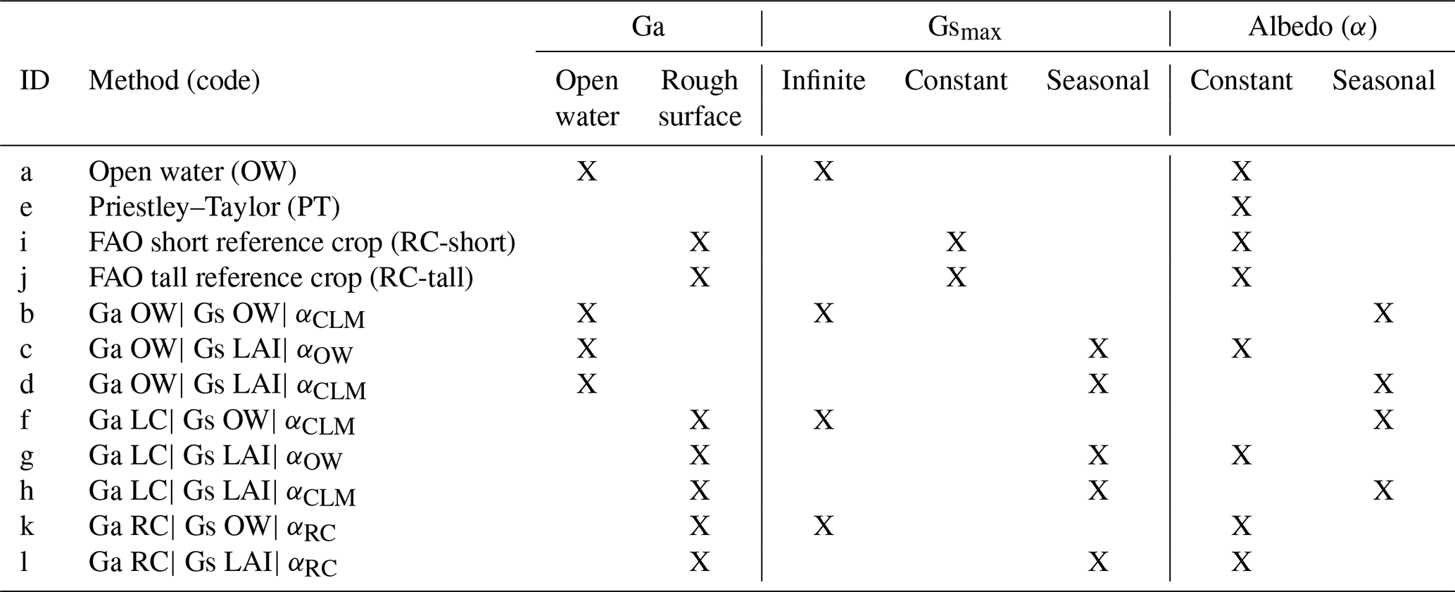
^* Note that many methods in these experiments are unrealistic due to inconsistencies in the surface conditions. Our aim is to include as many combinations as possible for a preliminary analysis.

In Sect. 5.1, we compare the CONUS-averaged R values between pairs of PET methods that share the same surface characteristics except for one feature (see Fig. 3). The first feature, surface roughness, is determined by the way Ga is estimated. We compare the parameter sets between rough and open-water surfaces by calculating the differences (rough surface minus open-water surface) for certain pairs of experiments, including (f) Ga LC| Gs OW| α_CLM minus (b) Ga OW| Gs OW| α_CLM; (g) Ga LC| Gs LAI| α_OW minus (c) Ga OW| Gs LAI| α_OW; and (h) Ga LC| Gs LAI| α_CLM minus (d) Ga OW| Gs LAI| α_CLM. In terms of surface conductance, we calculate the differences between seasonal and infinite Gs_max (seasonal Gs_max minus infinite Gs_max) for the following pairs of experiments: (c) Ga OW| Gs LAI| α_OW minus (a) OW; (d) Ga OW| Gs LAI| α_CLM minus (b) Ga OW| Gs OW| α_CLM; and (h) Ga LC| Gs LAI| α_CLM minus (f) Ga LC| Gs OW| α_CLM. We also compare the differences between all consistent and inconsistent surfaces and between seasonal and constant albedo.

4.3 Comparison of PET parameterizations

Based on the results of Sect. 5.1, we further examine different parameterizations for Ga and Gs in order to identify optimal PET algorithms (Table 4; results given in Sect. 5.2). We establish a control scenario where PET is not considered at all in the SPEI, equivalent to the traditional SPI. The PET methods under consideration fall into two categories: the big-leaf model and the two-source model. The big-leaf model includes three traditional methods (the open-water (OW), short-reference-crop (RC-short), and tall-reference-crop (RC-tall) methods), LC-dependent methods, and CH-dependent methods. The LC method uses the same aerodynamic conductance method (Eq. 9) but varies in terms of surface conductance parameterizations: the LC-K method adopts Gst_max from Kelliher et al. (1995), and the LC-Z method uses Rst_min from Zhou et al. (2006). The CH method also has two parameterizations: the CH-K and CH-Z methods. We then calculate ΔR between each PET method and the control scenario (where PET is set to zero).

Table 4 Summary of PET methods, including their formulas and parameterizations.

5 Results

5.1 Initial assessment of surface characteristics

We conducted a preliminary analysis to identify the relative importance of different surface characteristics. We examined eight algorithms to isolate the effects of surface characteristics on PET (Table 2). Figure 2 displays the spatial patterns of growing-season averages for these methods. For the classical Penman and Penman–Monteith methods (Fig. 2a, i, and j), the highest mean AED values for the growing season are found in southern California, Arizona, and Texas, while the PT method (Fig. 2e) predicts the largest AED values for Texas and Florida. The spatial patterns of PET based on the rough surface (rough Ga; Fig. 2f–h) are very different from those from methods that assume a universal reference height (reference crop; Fig. 2i–j) or an open-water surface (Fig. 2a–d). Specifically, regions which exhibit large PET estimates (>250 mm month⁻¹; Fig. 2h–k) are forests, such as evergreen needleleaf forests in the Pacific Northwest, deciduous needleleaf forests in the northeastern US, and mixed forests in the southeastern US. Interestingly, although methods using a constant albedo value (α=0.08) have generally larger AED values than those using seasonal albedo values, the differences in spatial patterns between the two are almost negligible (compare Fig. 2c and d and Fig. 2g and h). The combination of rough aerodynamic and unconstrained surface conductance, represented in method (f), produces extremely high monthly PET values, with means ranging from 330 to 340 mm month⁻¹. The remaining methods also predict a wide range of mean monthly totals.

Figure 2 Growing-season averages of AED derived from four PET methods and eight testing algorithms over the CONUS. Details and IDs for the methods are listed in Table 2.

Assessing the changes between pairs of these methods can identify whether adding/removing a surface feature eventually causes an improvement in drought quantification (Fig. 3). For a 1-month timescale, surface roughness stands out as the most important feature for enhancing the skill of the drought index (ΔR=0.01–0.025). Interestingly, for a 6-month timescale, activating realistic surface roughness does not necessarily increase the correlation with SMsurf, while activating dynamic surface conductance improves the correlation, meaning that adding plant phenology driven by the LAI can improve seasonal variations in the drought index over longer timescales. When comparing ΔR for inconsistent surfaces (e.g., a combination of open-water Ga and seasonal Gs) against ΔR for consistent surfaces, we find that methods with consistent surface features persistently show higher correlations with SMsurf (ΔR=0–0.02). Given the consistently better performance, we only focus on the consistent surface approaches in the subsequent sections. Surprisingly, seasonal and constant albedo showed no significant difference with regard to the correlations, possibly due to the little variation in albedo during the growing season. The differences in spatial patterns between constant and seasonal albedo are almost negligible (Fig. 2). In the subsequent sections, we default to using seasonal albedo in our PET methods to fully represent the surface characteristics.

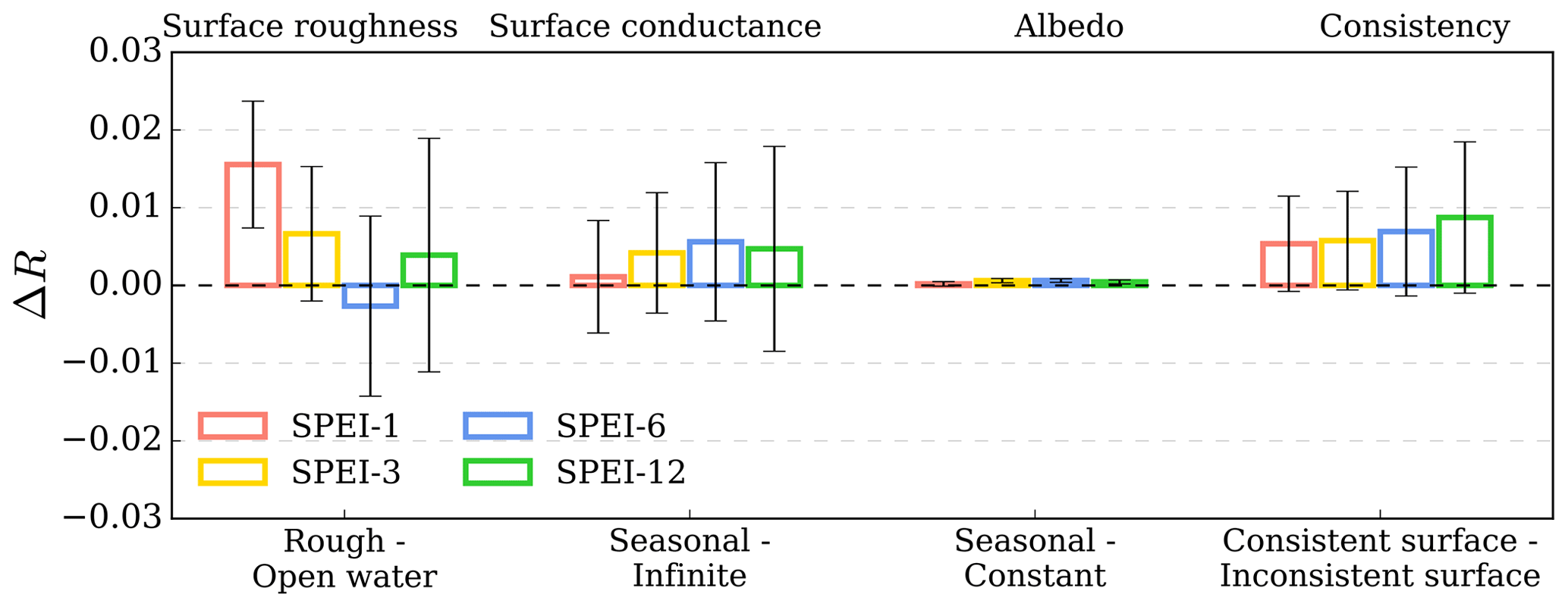
Figure 3 Differences in spatially averaged correlation (ΔR) for pairs of PET methods that share the same surface characteristics, except for one surface feature: surface roughness, surface conductance, albedo, or overall consistency among these features.

5.2 Performance of PET parameterizations

Figure 4 shows the ΔR values for each PET method listed in Table 4 and the control scenario (where PET is set to zero) for all grids, forested grids, and nonforested grids using the 1-month SPEI. Incorporating the benchmark OW method into the SPEI increases R by 0.042, indicated by the top horizontal bars. Among the conventional PET methods, the tall-reference-crop (RC-tall) method stands out. Over the CONUS, it improved ΔR relative to the control scenario by 29 % more than the OW method (0.054 versus 0.042). The short-reference-crop (RC-short) method has an identical averaged R to that of the OW method. Although the RC-tall algorithm (Allen et al., 2005) is less known than the widely used RC-short algorithm (Allen et al., 1998), our results suggest that the SPEI driven by the RC-tall method correlates better with SMsurf dynamics.

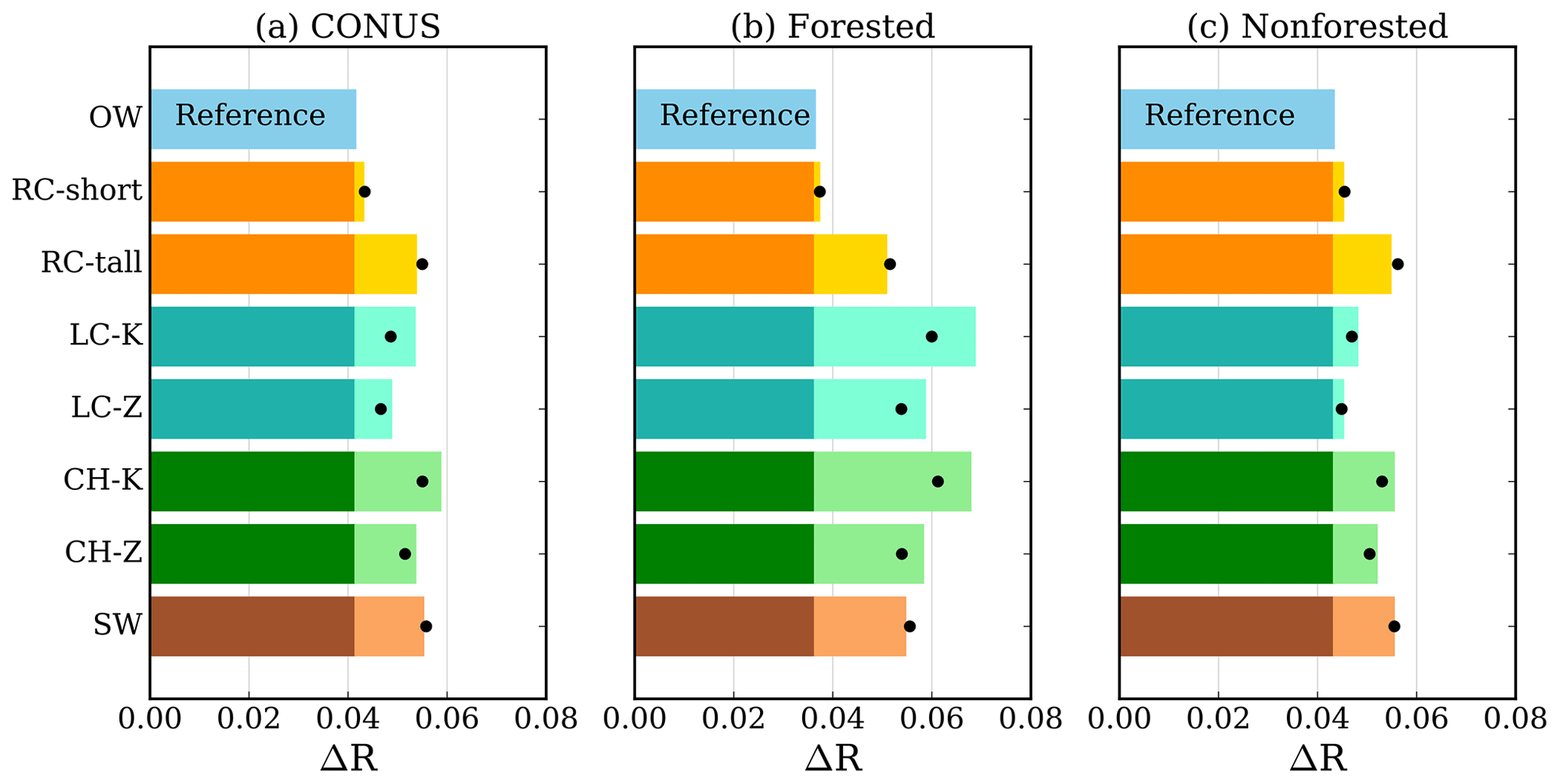
Figure 4 Differences in correlation (ΔR) for selected PET methods versus the control scenario (where PET is set to zero). Correlations were computed between the 1-month SPEI and SMsurf series across (a) the CONUS, (b) forested grids, and (c) nonforested grids. The bars represent the mean ΔR, and the black dots represent the median ΔR. The top blue bars show ΔR in the OW approach versus a PET value of zero as a reference. For each bar, the darker shade indicates the reference ΔR, and the lighter shade represents any improvement (or decline) relative to the reference.

One encouraging outcome is the performance improvement seen in the two big-leaf LC and CH algorithms incorporating realistic surface conductance. Activating both surface roughness and seasonal Gs produces high correlations between the SPEI and SMsurf. These algorithms improve the OW method (ΔR=0.042) by 29 %–41 % (ΔR=0.053–0.059). Methods where Ga is determined by the canopy height (green bars in Fig. 3a) especially improve correlations with SMsurf. Methods where Gs is determined by Eq. (14) and parameterized using Kelliher et al. (1995) produce higher correlations in both the LC and CH algorithms. This confirms our hypothesis that incorporating realistic vegetation information into atmospheric evaporative demand can enhance drought characterization. Finally, the two-source Shuttleworth–Wallace (SW) method outperforms the OW method, as expected. However, the SW method produces a smaller R value than the CH-K method. This suggests that the simple big-leaf model combined with land cover details can achieve the same efficacy as the more complicated two-source model.

Over the CONUS, the RC-tall, LC-K, CH-K, and SW methods come out on top, exhibiting similar average R values. However, when we evaluate the performance in forested areas (Fig. 3b), the LC-K and CH-K methods exhibit the most significant improvement in ΔR compared to the control scenario, with increases of 86 %–89 % in comparison to the OW method's improvement (0.068 relative to 0.036). The RC-tall and SW methods improve ΔR relative to the control scenario by 39 % (0.05) and 50 % (0.054), respectively. In nonforested areas (Fig. 3c), the RC-tall method has the best performance, followed by the SW and CH-K methods. The SW method, designed for sparse vegetation, naturally demonstrates strong performance in these regions. Similarly, the CH-K method uses the dataset by Lang et al. (2023), which includes higher-quality canopy height measurements in short vegetated areas. Conversely, the LC-K method only exhibits a moderate improvement in ΔR. This suggests that the performance of the land-cover-based approach in sparse vegetation is strongly influenced by the uncertainty in the roughness parameters. On the other hand, it is surprising to see that the simple parameterized RC-tall method can outperform the SW method. This suggests that, particularly in sparsely vegetated areas, the RC-tall method can serve as a strong yet simple approach for PET estimates and drought characterization.

5.3 Spatial-pattern analysis

In the subsequent sections, we compare the LC-K and CH-K methods (hereafter referred to as the LC and CH-K methods), along with the RC-tall and SW approaches, against three widely used methods: the OW, PT, and RC-short methods. The time series for these PET methods, as well as the SMsurf time series, are shown in Fig. 5. The spatial patterns of the mean monthly PET values are shown in Fig. C1 (Appendix C). The OW approach serves as the reference. The highest R values are observed for long-term drought (12 months; average R value of 0.73), and the lowest are found for medium-term drought (3 and 6 months; average R value of 0.48). This suggests that the meteorology-driven SPEI can generally reproduce soil moisture dynamics, especially on an annual timescale.

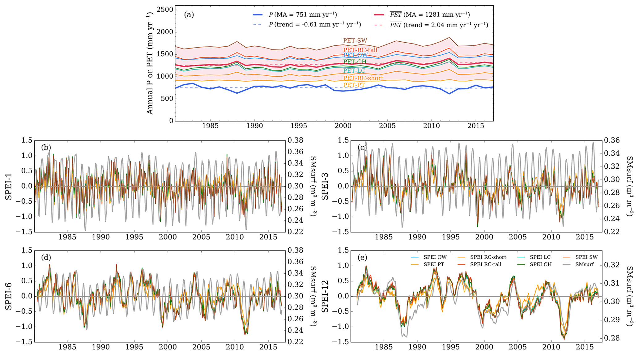
Figure 5 Temporal evolution of PET methods, SPEIs, and SMsurf. (a) Annual precipitation and PET (mm yr⁻¹) from PET methods between 1981–2017. (b–e) SPEI series driven by the PET methods, aligning with the SMsurf time series for four timescales (1, 3, 6, and 12 months). MA: multi-year average.

Figure 6 displays the spatial distribution of correlations between the SPEI driven by the OW method and SMsurf, along with the differences in the correlations of the PT, RC-short, RC-tall, LC, CH, and SW methods compared to the OW approach. The PT method consistently exhibits lower correlations than the OW approach over most regions, with an average decrease of 0.04, and shows especially weak correlations in the southwestern US (lower by 0.15). Interestingly, the widely used RC-short method for the SPEI presents little improvement compared to the OW method, with minimal increases in correlation, while the RC-tall method demonstrates an overall better performance across the CONUS and various timescales. Both the CH and LC methods show substantial improvements in some areas, with ΔR exceeding 0.16, particularly in the eastern US and Pacific Northwest. The enhancements of the LC and CH methods are prominent, but they can be diluted when averaged across the CONUS, with ΔR relative to the control scenario being 0.012 higher than that for the OW method (Fig. 4a). This is especially true when considering their less favorable performance in the southwestern and midwestern US. The SW method also exhibits notable improvements in the eastern US and Pacific Northwest, with a magnitude of improvement falling between that of the CH and RC-short methods. It is encouraging to see that the LC and CH methods outperform the SW method in many eastern US grid cells (ΔR=0.15 versus ΔR=0.05), given their much simpler parameterizations. However, it is worth noting that the LC, CH, and SW approaches experience performance declines in the southwest, with the LC and CH methods performing slightly worse than the SW method. On the other hand, the RC-tall method robustly displays improvements in this particular area.

Figure 6 The first row displays the correlations between the SPEI driven by the OW method and SMsurf. The rows below show the differences in correlation (ΔR) for the PET methods relative to the OW method.

We further delve into the relative performance of the top four methods, summarized according to the major vegetation types and aridity (Fig. 7). Both the LC and CH methods show significantly increased R values in forests, especially in evergreen broadleaf forests, deciduous broadleaf forests, and mixed forests, where the largest ΔR value exceeds 0.1 and the average ΔR value hovers around or above 0.05 at a 1-month timescale (Fig. 7a). Notable improvements compared to the OW method are also observed in evergreen needleleaf forests, woody savannas, croplands, and mosaic lands. The LC approach performs slightly better than the CH approach in forests, while the CH approach performs slightly better in shorter vegetation.

For the timescale of 12 months (Fig. 7c), the OW method already has a high average R value of 0.73 across the CONUS. The LC and CH methods' performance is outstanding in forests, with an average ΔR value of about 0.05 and the largest ΔR value exceeding 0.25. In evergreen needleleaf forests, the CH and LC methods' performance is significantly higher than that at the 1-month timescale. In humid regions, the improvements of the CH and LC methods relative to the SW method become even more apparent when compared to the 1-month timescale (Fig. 7d).

Figure 7 Violin plots illustrating the differences in correlation for three PET methods relative to the OW method, categorized according to the vegetation type and aridity. In each violin plot, the black dot represents the median, and the black line represents the mean.

In contrast, the average performance of the LC and CH methods in grasslands, shrublands, and savannas (Fig. 7a and c), which are the dominant vegetation types in the western CONUS, is equivalent to or slightly lower than that of the OW method. The magnitude of averaged ΔR for the LC and CH methods is slightly smaller than that for the RC-tall and SW methods, mainly due to their weaker performance in arid shrublands and grasslands, which cover large portions of the CONUS. The more complicated LC, CH, and SW methods show less advantage or even worse performance compared to the RC-tall and OW methods in nonforested and arid grid cells (Fig. 7c–d).

6 Discussion

6.1 Interaction between surface features

Figure 3 provides important insights into the sensitivity of the SPEI to different surface features. Introducing Gs with seasonal vegetation dynamics accounts for most of the total improvement in the PET algorithm. This confirms that the FAO approaches are favored over the OW approach due to their constraints on Gs. This highlights the importance of the leaf area index (LAI) as a vegetation feature for drought depiction. The LAI serves as a scaling factor for upscaling Gst_max to maximum canopy conductance. This differs from drought indices based on the normalized difference vegetation index (NDVI) or LAI, which require real-time dynamics of satellite data. This approach only requires the climatology of the LAI, which can be easily implemented for drought forecasting where real-time or near-future data are not available.

Using realistic surface roughness does not necessarily improve the overall performance of the SPEI. In fact, the consistency between aerodynamic conductance and surface conductance is more critical for the skill of PET method. A previous study by Peng et al. (2019) explains the linkage between the ratio of actual ET to PET and the ratio of Ga to Gs. When Ga $/$ Gs is large, the ratio of actual ET to PET becomes smaller. Although our study focused on maximum evapotranspiration under realistic vegetation conditions, such a relationship remains valid. Thus, a large Ga $/$ Gst_max ratio should better limit PET with realistic surface constraints. In fact, the LC approach activates surface roughness and increases Ga while constraining Gst_max and reducing Gs; the CH approach further incorporates canopy height and the LAI in the representation of surface roughness. Altogether, these factors increase the Ga $/$ Gs ratio and result in significant improvement in capturing the temporal evolution of SMsurf.

6.2 Surface characteristics matter in forests

Our analysis concludes that incorporating surface features can largely improve the accuracy of drought monitoring in forests. There are two vegetation groups that show significantly improved correlations after incorporating realistic surface characteristics. For forests in the eastern and western US, such as evergreen and deciduous broadleaf forests, the LC and CH methods exhibit large ΔR values compared to the OW method (up to 0.12 for 1 month and up to 0.25 for 12 months; Fig. 7a and c). While the OW method has a ΔR value of about 0.036 compared to the zero-PET control scenario (Fig. 4b), the LC method has an average ΔR value of 0.032 relative to the OW method with respect to these forests. This means that the improvement of the LC method compared to the control scenario is almost double that of the OW method. The CH and LC methods also display a significant increase in R of about 0.025 for woody savannas. The enhancements in forests and woody savannas are the most predominant since the LAI is relatively variable for forests, where surface roughness is also the strongest. Although the southeastern US has a humid subtropical climate, this region suffered from periodic droughts in 1986–1988, 1998–2002, and 2006–2009 (Seager et al., 2009; Pederson et al., 2012), consistent with the increased forest drought severity from 1987–2013 (Peters et al., 2014; Clark et al., 2016). Drought monitoring in these regions is also critical and can benefit from our approach, which significantly improves spatial and temporal accuracy in forests.

In contrast, short-grass regions (grasslands, shrublands, and savannas) located in the western US exhibit minimal improvements in the LC method. The CH method, incorporating the newly available Lang et al. (2023) canopy height dataset, improves correlations across grasslands, croplands, and mosaic lands. Given that the RC-tall method – a similar big-leaf model – performs better than the LC and CH methods in shrublands (Figs. 4 and 7), uncertainties in Gst_max from the LC and CH methods could result in these outcomes. Additionally, a comparison between Gst_max and Rst_min (used in the SW method) highlights uncertainties in this parameter. For instance, Rst_min in shrublands, grasslands, and savannas ranges from 100–180 s m⁻¹ (equivalent to a Gst_max value of 5–10 mm s⁻¹), which is generally lower than the 9–12 mm s⁻¹ range reported by Kelliher et al. (1995). These findings highlight the need for in situ measurements of surface conductance in these areas.

Furthermore, these areas have sparse vegetation cover, and, thus, the LAI plays a less effective role in determining the seasonal dynamics of PET. In the meantime, while these areas are located in arid regions (Fig. 7), improvements in PET do not have a significant effect on modeling soil moisture, and precipitation dynamics may dominate soil moisture variations.

6.3 Strategies for PET method selection

Both the CH and LC methods not only provide modest absolute PET values (Figs. 5a and C2), but also display better performance across many areas (Fig. 6). Specifically, the LC and CH methods estimate an annual PET of roughly 1200 mm, which falls within the range between the higher OW value (1424 mm) and the lower values around 1100 mm from the RC-short method and the Sun et al. (2023) PET dataset (Fig. C2).

As Ershadi et al. (2015) pointed out, no single model consistently outperforms others across all land cover types. The selection of PET for model simulation varies depending on the region (Pimentel et al., 2023). We recommend the use of both LC and CH parameterizations for drought monitoring in forests, where the roughness and surface conductance parameters vary with realistic vegetation conditions. Both are superior to the OW and RC-short parameterizations because of their better performance. Additionally, compared to the SW parameterizations, both perform better and are simpler approaches for forested areas. Between the CH and LC approaches, we recommend the CH approach because it factors in the dynamic change in vegetation structure and provides slightly better performance in woody savannas.

For shrublands and grasslands, we recommend using the RC-tall approach instead of the more widely used RC-short approach for drought monitoring. We found that the RC-tall approach has a higher skill than the RC-short approach, which is more widely used. The main difference between these two methods is the C_n constant, which describes the effect of aerodynamic conductance (Allen et al., 2005). The implementation of a tall reference (C_n=1600) seems to work better than that of a short reference (C_n=900) across the CONUS. It is worth noting, however, that the FAO approaches assume a universal C_n regardless of the actual vegetation type. The better skill of the RC-tall approach may not always hold, leading to potential overestimation of PET in semiarid nonvegetated regions.

For sparse vegetation, since the responses of evapotranspiration components to environmental drivers are different (Katul et al., 2012; Or and Lehmann, 2019), the partitioning between canopy and soil can also play a role in determining AED. The SW model significantly improves the SPEI skill driven by the OW approach. It outperforms the LC and CH methods in croplands and grasslands. Despite its complexity, it is a good choice for drought monitoring in these vegetation types (Sun et al., 2023).

For croplands, we recommend choosing between the RC-tall and RC-short methods, which are based on the actual crop canopy height. The more realistic approach is to use the RC-tall method for taller crops. Lastly, the PT method has the poorest correlation with soil moisture and is unlikely to capture drought dynamics.

6.4 Bridging gaps in drought prediction

Motivated by the question of whether incorporating surface characteristics can improve drought prediction, we address several limitations of previous drought quantification methods. Firstly, our study presents a different approach by focusing on the maximum possible evapotranspiration for a given vegetation condition. This concept allows for a physically meaningful definition of evaporative demand for nonuniform land surfaces.

Secondly, the ultimate goal of PET calculation is to simulate ET and quantify drought. Despite the simplicity of calculating PET using existing Penman-type methods, the biggest challenge when assessing these methods concerns validation. Since the real evaporative-demand rate is unattainable from observations, it is challenging to validate which PET method is superior directly. Even using ET observations for PET validation can be problematic because biased PET estimates and incorrect surface biophysical parameters can still produce accurate ET estimates for locations with ET measurements (Peng et al., 2019). Our study evaluates PET methods by comparing drought indices with independently observed soil moisture (Vicente-Serrano et al., 2012). This approach helps directly diagnose the most appropriate PET approach for drought quantification while avoiding the complexity and divergence caused by various PET definitions. Although the absolute improvements in the correlation with soil moisture appear modest, they represent significant percentage changes of 25 %–30 % on average and notable local improvements of 86 %–89 % in forests. We acknowledge the need to evaluate effectiveness in addition to temporal correlations. Specifically, future studies should evaluate the capability of land-cover-specific approaches to accurately capture extreme events.

Finally, our approach bridges the gap between two methodologies for quantifying soil moisture drought, which is of most relevance to agriculture (Seneviratne, 2012). Since soil moisture observations are limited by inadequate measurement networks, drought indices, such as the SPEI, are often used to quantify drought. In hydrology, a drought index is a simple water balance model driven by surface meteorology that does not use any surface characteristics. Its shortcomings include neglecting seasonally varying vegetation cover and its inability to capture vegetation control on transpiration. An alternative is to use land surface models to estimate large-scale soil moisture (Sheffield and Wood, 2007). This approach often incorporates vegetation dynamics and can provide temporally consistent soil moisture simulations, but it also requires substantial effort to prepare meteorological forcings at a high temporal resolution, set up the domain, conduct spinup, and perform calibrations. Our approach is a compromise between these two types of models, offering a more realistic and process-based alternative to the commonly used drought index while being easier to implement and less data-intensive than a land surface model.

7 Conclusions

To understand whether incorporating surface characteristics can improve drought prediction, we revise current PET methods in a newly developed drought index (SPEI) using the concept of maximum ET for any given vegetation condition. We use a simple lookup table approach that combines in situ measurements and large-scale data fusion products for the key surface and aerodynamic parameters. This study also presents a novel application of independent soil moisture observations to diagnose the most appropriate PET approach for drought quantification. Our approach has been shown to be more effective than widely used big-leaf methods and two-source models in accurately predicting soil moisture spatiotemporal dynamics in forests and humid regions. This new yet simple approach strikes a balance between a meteorology-driven water balance model and a complex land surface model for drought prediction. It could improve the accuracy of drought reconstruction in forests, and it displays great potential with regard to improving real-time drought forecasts.

Appendix A: Shuttleworth–Wallace model

The two-source Shuttleworth–Wallace (SW) model was developed to more accurately represent evapotranspiration from sparse vegetation. Unlike the big-leaf models, the SW model treats the surface as a two-component structure consisting of sparse vegetation (e.g., row crops) and soil. The following formulas are adapted from Eqs. (11)–(18) in Shuttleworth and Wallace (1985).

$$\begin{array}{}\text{(A1)}& {\mathrm{PET}}_{\mathrm{SW}}=C_c{\mathrm{PET}}_{\mathrm{PM}}^{\mathrm{c}}+C_s{\mathrm{PET}}_{\mathrm{PM}}^{\mathrm{s}},\end{array}$$

where PET${}_{\mathrm{PM}}^{\mathrm{c}}$ and PET${}_{\mathrm{PM}}^{\mathrm{s}}$ are Penman–Monteith-like combined equations (Eq. 4) for a closed canopy and bare soil. The terms are given by the following formulas:

$$\begin{array}{}\text{(A2)}& {\displaystyle }{\mathrm{PET}}_{\mathrm{PM}}^{\mathrm{c}}={\displaystyle \frac{\begin{array}{c}\mathrm{\Delta }\left(R_{\mathrm{n}}-G\right)+({\mathit{\rho }}_a{C}_{p}D-\mathrm{\Delta }{r}_{\mathrm{a}}^{\mathrm{c}}(R_{\mathrm{n}}^{\mathrm{s}}-G\left)\right)/\\ (r_{\mathrm{a}}^a+r_{\mathrm{a}}^{\mathrm{c}})\end{array}}{\mathit{\lambda }\left(\mathrm{\Delta }+\mathit{\gamma }\left(\mathrm{1}+\frac{r_{\mathrm{s}}^{\mathrm{c}}}{r_{\mathrm{a}}^a+r_{\mathrm{a}}^{\mathrm{c}}}\right)\right)}},\text{(A3)}& {\displaystyle }{\mathrm{PET}}_{\mathrm{PM}}^{\mathrm{s}}={\displaystyle \frac{\begin{array}{c}\mathrm{\Delta }\left(R_{\mathrm{n}}-G\right)+({\mathit{\rho }}_a{C}_{p}D-\mathrm{\Delta }{r}_{\mathrm{a}}^{\mathrm{s}}(R_{\mathrm{n}}-R_n^{\mathrm{s}}\left)\right)\\ /(r_{\mathrm{a}}^a+r_{\mathrm{a}}^{\mathrm{s}})\end{array}}{\mathit{\lambda }\left(\mathrm{\Delta }+\mathit{\gamma }\left(\mathrm{1}+\frac{r_{\mathrm{s}}^{\mathrm{s}}}{r_{\mathrm{a}}^a+r_{\mathrm{a}}^{\mathrm{s}}}\right)\right)}},\text{(A4)}& {\displaystyle }{C}_c={\displaystyle \frac{\mathrm{1}}{\mathrm{1}+\frac{R_c{R}_a}{R_s\left(R_c+R_a\right)}}},\text{(A5)}& {\displaystyle }{C}_s={\displaystyle \frac{\mathrm{1}}{\mathrm{1}+\frac{R_s{R}_a}{R_c\left(R_s+R_a\right)}}},\text{(A6)}& {\displaystyle }{R}_a=\left(\mathrm{\Delta }+\mathit{\gamma }\right)r_{\mathrm{a}}^a,\text{(A7)}& {\displaystyle }{R}_s=\left(\mathrm{\Delta }+\mathit{\gamma }\right)r_{\mathrm{a}}^{\mathrm{s}}+\mathit{\gamma }{r}_{\mathrm{s}}^{\mathrm{s}},\text{(A8)}& {\displaystyle }{R}_c=\left(\mathrm{\Delta }+\mathit{\gamma }\right)r_{\mathrm{a}}^{\mathrm{c}}+\mathit{\gamma }{r}_{\mathrm{s}}^{\mathrm{c}},\end{array}$$

where many terms are defined by Eqs. (1)–(2), except the following: $R_{\mathrm{n}}^{\mathrm{s}}$ represents net radiation over the soil surface, $R_{\mathrm{n}}^{\mathrm{s}}\left(\mathrm{1}-f_{\mathrm{veg}}\right)=R_{\mathrm{n}}^{\mathrm{s}}\cdot \exp (-\mathrm{0.5}\cdot \mathrm{LAI})$, $r_{\mathrm{a}}^{\mathrm{a}}$ represents aerodynamic resistance between the canopy height and reference level (s m⁻¹), $r_{\mathrm{s}}^{\mathrm{s}}$ represents surface resistance of the substrate (s m⁻¹), $r_{\mathrm{a}}^{\mathrm{s}}$ represents aerodynamic resistance between the substrate and canopy (s m⁻¹), $r_{\mathrm{s}}^{\mathrm{c}}$ represents bulk stomatal resistance of the canopy (s m⁻¹), and $r_{\mathrm{a}}^{\mathrm{c}}$ represents bulk boundary layer resistance of the vegetative elements in the canopy (s m⁻¹).

In this study, the resistances are parameterized for feasible minimal values based on the water-unlimited assumption for estimating PET. The substrate resistance ($r_{\mathrm{s}}^{\mathrm{s}}$) is set to 0 s m⁻¹ as a saturated surface. The canopy resistances are dependent on the LAI (Eqs. 19–20 in Shuttleworth and Wallace (1985)).

$$\begin{array}{}\text{(A9)}& {\displaystyle }{r}_{\mathrm{s}}^{\mathrm{c}}=\mathrm{Rst}\cdot {\displaystyle \frac{\mathrm{1}}{{\mathrm{LAI}}_{\mathrm{e}}}}\text{(A10)}& {\displaystyle }{r}_{\mathrm{a}}^{\mathrm{c}}=r_{\mathrm{b}}\cdot {\displaystyle \frac{\mathrm{1}}{\mathrm{2}\mathrm{LAI}}}\end{array}$$

Stomatal resistance (Rst) is set to the Rst_min values obtained by the land cover types in Table 1. The effective leaf area index (LAI_e) corresponds to LAI/2 and is capped at 2 (even when the LAI is greater than 4). Note that $r_{\mathrm{s}}^{\mathrm{c}}$ does not have valid values for nonvegetated grid cells (at a specific time of the year or location). The leaf boundary layer resistance (r_b) is set to a value of 50 s m⁻¹ (Brisson et al., 1998).

The formulas for aerodynamic resistances are given as follows (Shuttleworth and Gurney, 1990; Zhou et al., 2006):

$$\begin{array}{}\text{(A11)}& {\displaystyle }\begin{array}{rl}{r}_{\mathrm{a}}^{\mathrm{s}}& ={\displaystyle \frac{h\cdot \exp \left(n\right)\ln \left(\frac{z_{\mathrm{m}}-d_{\mathrm{0}}}{z_{\mathrm{0}}}\right)}{n{k}^{\mathrm{2}}\left(h-d_{\mathrm{0}}\right)}}\left(\exp \left(-{\displaystyle \frac{n{z}_{\mathrm{0}\mathrm{g}}}{h}}\right)\right.\\ & \left.-\exp \left(-{\displaystyle \frac{n\left(z_{\mathrm{0}\mathrm{m}}+d_{\mathrm{p}}\right)}{h}}\right)\right),\end{array}\text{(A12)}& {\displaystyle }\begin{array}{rl}{r}_{\mathrm{a}}^a& ={\displaystyle \frac{\ln \left(\frac{z_{\mathrm{m}}-d_{\mathrm{0}}}{z_{\mathrm{0}}}\right)\ln \left(\frac{z_{\mathrm{m}}-d_{\mathrm{0}}}{h-d_{\mathrm{0}}}\right)}{k^{\mathrm{2}}{u}_z}}+{\displaystyle \frac{\ln \left(\frac{z_{\mathrm{m}}-d_{\mathrm{0}}}{z_{\mathrm{0}}}\right)h}{n{k}^{\mathrm{2}}(h-d_{\mathrm{0}})}}\\ & \left(\exp \left(n\left(\mathrm{1}-{\displaystyle \frac{z_{\mathrm{0}\mathrm{m}}+d_{\mathrm{p}}}{h}}\right)\right)-\mathrm{1}\right),\end{array}\end{array}$$

where h is the canopy height (m); k is the von Kármán constant; z_0m is the preferred roughness length (m); $z_{\mathrm{0}\mathrm{m}}=h/\mathrm{8}$; d_p is the preferred zero-plane displacement height (m); d_p=0.63h; z_0g is the roughness length of the ground (m); u_z is the wind speed from the measurement height (m s⁻¹); and z_m is the measurement height (m), assuming $z_{\mathrm{m}}=h+\mathrm{2}$.

Moreover, d₀ is the zero-plane displacement of the canopy (m), n is the eddy diffusivity decay constant of the vegetation, and z₀ is the canopy roughness length (m). These terms are parameterized as follows (Eqs. 22–26 in Zhou et al., 2006):

$$\begin{array}{}\text{(A13)}& {\displaystyle }n=\left\{\begin{array}{ll}\mathrm{2.5},& h\le \mathrm{1}\\ \mathrm{2.306}+\mathrm{0.194}h,& \mathrm{1}<h<\mathrm{10}\\ \mathrm{4.25},& h\ge \mathrm{10}\end{array},\right.\text{(A14)}& {\displaystyle }{d}_{\mathrm{0}}=\left\{\begin{array}{ll}h-z_{\mathrm{0}c}/\mathrm{0.3},& \mathrm{LAI}\ge \mathrm{4}\\ \mathrm{1.1}h\cdot \ln (\mathrm{1}+{\left(C_{\mathrm{d}}\mathrm{LAI}\right)}^{\mathrm{0.25}}),& \mathrm{LAI}<\mathrm{4}\end{array},\right.\text{(A15)}& {\displaystyle }{z}_{\mathrm{0}}=\min (\mathrm{0.3}\left(h-d_{\mathrm{0}}\right),z_{\mathrm{0}\mathrm{g}}+\mathrm{0.3}h{\left(C_{\mathrm{d}}\mathrm{LAI}\right)}^{\mathrm{0.5}}),\text{(A16)}& {\displaystyle }{C}_{\mathrm{d}}=\left\{\begin{array}{ll}\mathrm{1.4}\times {\mathrm{10}}^{-\mathrm{3}},& h=\mathrm{0}\\ \mathrm{0.25}{\left(-\mathrm{1}+\exp \left(\mathrm{0.909}-\frac{\mathrm{3.03}{z}_{\mathrm{0}c}}{h}\right)\right)}^{\mathrm{4}},& h>\mathrm{0}\end{array},\right.\text{(A17)}& {\displaystyle }{z}_{\mathrm{0}c}=\left\{\begin{array}{ll}\mathrm{0.13}h,& h\le \mathrm{1}\\ \mathrm{0.139}h-\mathrm{0.009}{h}^{\mathrm{2}},& \mathrm{1}<h<\mathrm{10}\\ \mathrm{0.05}h,& h\ge \mathrm{10}\end{array},\right.\end{array}$$

where z_0c is the roughness length for a closed canopy (m) and C_d is the mean drag coefficient for individual leaves.

Appendix B: Canopy height data

We evaluated the newly available global canopy height dataset (Lang et al., 2023) and the widely used global tree height dataset (Simard et al., 2011). Although the datasets are highly consistent with each other (Fig. B1), some discrepancies exist for low-vegetation cases, which is expected due to the fact that Simard et al. (2011) focused on tree height estimates. We further compared the histogram of canopy height across different land cover types between Lang et al. (2023; Fig. B2) and Simard et al. (2011; Fig. B3). The two datasets are highly consistent in forests, while Lang et al. (2023) provides valuable information for short vegetation types.

Figure B1 Comparison of canopy height between Lang et al. (2023) and Simard et al. (2011). RMSE: root mean square error.

We reconstruct the canopy height in each grid cell by comparing the value in Lang et al. (2023) with the ranges given for the land cover type. If it is outside the range (smaller than h_min or greater than h_max), we assign the grid cell a typical value of canopy height (h_typ). For forests, we continue to follow the definitions from the IGBP land cover classification, which specify that forests are taller than 2 m. This supersedes the range given in Lang et al. (2023), which provides a range of values less than 2 m. Typical canopy height is taken from the value of the peak (mode) rather than the median for forests. For deciduous broadleaf forests, Lang et al. (2023) only has three data points, meaning we instead use the distribution of Simard et al. (2011) while keeping the lower limit of 6 m from Lang et al. (2023). For grasslands, wetlands, and croplands, the lidar estimates from Lang et al. (2023) or Simard et al. (2011) are typically more than 3–5 m, possibly due to overestimation of the grid cell by sampling tall trees. Considering the difficulties in separating trees from grass and pastures, we did not adopt the high canopy height values for these land cover types. We use conservative estimates from the literature: 1.5 m (mean value of 0–3 m) for grasslands and 0.5 m for wetlands.

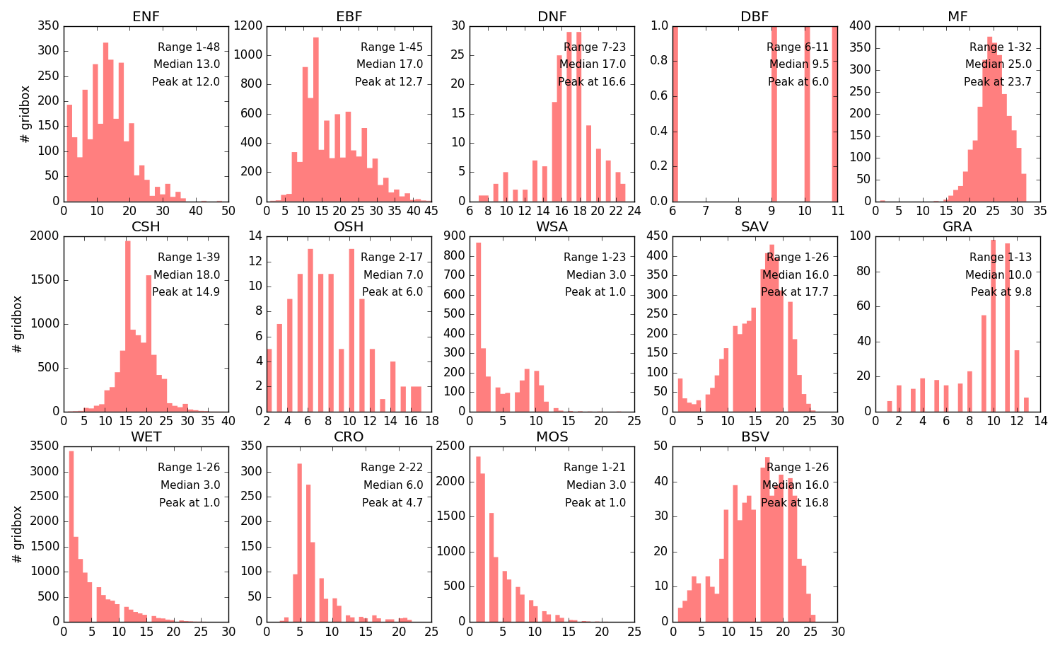
Figure B2 Histograms of canopy height (Lang et al., 2023), categorized according to land cover type, for the CONUS (nonvegetated land cover types, i.e., URB, MOS, and SNO, are excluded).

Figure B3 Histograms of tree height (Simard et al., 2023), categorized according to forest type, for the CONUS.

Appendix C: Comparison of multiple PET datasets (mm month⁻¹)

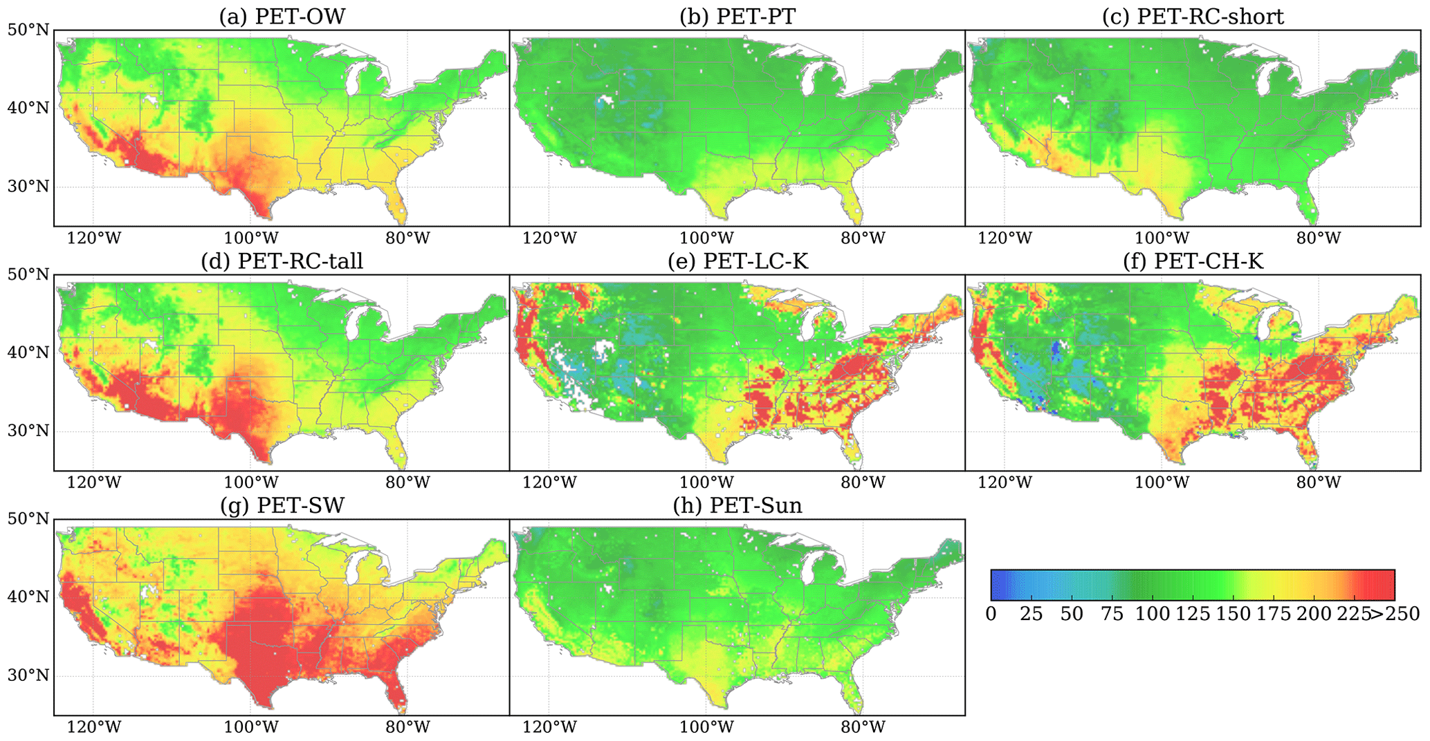
Figure C1 Growing-season averages of the PET methods used in this study (Table 4) and the PET dataset from Sun et al. (2023) for the CONUS.

Figure C2 Annual times series of the PET methods used in this study (Table 4) and the PET dataset from Sun et al. (2023) for the CONUS.