Projected changes in land carbon store over the 21st century: what contributions from land use change and atmospheric nitrogen deposition?

Earth system models (ESMs) represent the time evolution of the biophysical (energy and water cycles) and biogeochemical (carbon cycle) components of the Earth. When used for near-future projections in the context of the Coupled Model Intercomparison Project (CMIP), they use as forcings the evolution of greenhouse gas and other pollutant concentrations and land use changes simulated by an ensemble of integrated assessment models (IAMs) for a combination of socioeconomic pathways and mitigation targets (SSPs). More precisely, only one IAM output is used as representative of a single SSP. This makes the comparison of key ESM diagnostics among SSPs significantly noisy and without the capacity of disentangling SSP-driven and IAM-driven factors. In this paper, we quantify the projected change in land carbon store (CLCS) for the different SSPs with an advanced version of a land surface model embedded into IPSL-CM6 ESM. Through a set of land-only factorial simulations, we specifically aim at estimating the CLCS dispersions associated with land use change and nitrogen deposition trajectories. We showed that the spread of the simulated change in global land carbon store induced by the uncertainty in the land use changes is slightly larger than the one associated with the uncertainty in the atmospheric CO₂. Globally, the uncertainty associated with N depositions is responsible for a spread in CLCS that is lower by a factor of 3 than the one driven by atmospheric CO₂ or land use changes. Our study calls for making available additional IAM scenarios for each SSP to be used in the next CMIP exercise in order to specifically assess the IAM-related uncertainty impacts on the carbon cycle and the climate system.

1 Introduction

In the framework of Phase 6 of the Coupled Model Intercomparison Project (CMIP6), the ScenarioMIP experiments (O'Neill et al., 2016) address the near-future evolution (2015–2100) of the Earth system for a combination of socioeconomic and climate policy scenarios. Five Shared Socioeconomic Pathways (SSPs) are explored (Riahi et al., 2017) with contrasting assumptions regarding the future evolution of society in terms of population growth, economic development, urbanisation, and other factors. Driven by these five socioeconomic pathways, an ensemble of integrated assessment models (IAMs) simulates the evolution of energy and land use systems and the associated emissions of greenhouse gases (GHGs) and other pollutants. In the context of ScenarioMIP, a selection of simulations is performed for the five socioeconomic pathways with or without a mitigation strategy (baseline scenario) leading to specific radiative forcings in 2100 (O'Neill et al., 2016). As defined in O'Neill et al. (2016), we label these eight scenarios as SSPx-y, with x as the inter-selected SSP and y as the 2100 radiative forcing. Hereafter, we refer to these scenarios as SSPs for simplicity. In order to be used by Earth system models (ESMs), IAM outputs are harmonised to be consistent with the data used for the historical period and downscaled from the IAM large-region scale to a finer-gridded one. Harmonisation and downscaling are performed for land use (Hurtt et al., 2020) and for emissions of GHGs and other atmospheric compounds impacting climate such as ammonia or nitrogen oxides (Feng et al., 2020; Gidden et al., 2019).

Most of the CMIP6 experiments designed to assess the contemporary evolution of the Earth system have been performed in a so-called concentration-driven mode. In such a configuration, atmospheric CO₂ concentration ([CO₂]) is imposed, and fossil CO₂ fuel emissions are computed a posteriori as the remaining flux compatible with the time evolution of [CO₂] and the net land–atmosphere and ocean–atmosphere CO₂ fluxes. Liddicoat et al. (2021) computed the compatible fossil fuel CO₂ emissions deduced from the historical and ScenarioMIP experiments of nine ESMs. They showed that the multimodel mean cumulative compatible fossil fuel CO₂ emissions over 1850–2100 were in close agreement with the estimate based on observation (for the historical period) and the IAMs (for the period 2015–2100) for the different SSPs. The absolute relative difference between the multimodel mean and the observation-/IAM-based estimate ranges from 1 % (for SSP3-7.0) to 13 % (for SSP1-1.9), proving the overall good consistency between ESM and IAM carbon (C) cycle modelling. However, the model spread is large, with an intermodel standard deviation (SD) ranging from 5 % (for SSP5-8.5) to 15 % (for SSP4-3.4) of the multimodel mean compatible fossil fuel CO₂ emissions. This large disagreement between ESMs is primarily attributable to the land carbon response, with an intermodel standard deviation for the land carbon store between 1850 and 2100 of the order of 67 % of the multimodel mean, while the one for the ocean carbon store does not exceed 6 %.

In this context, our paper focus on the projected ESM land carbon store for the different SSPs and in particular on an additional source of uncertainty related to the IAM forcings. Indeed, five IAMs simulated the evolution of the energy and land use systems and associated gas emissions for each SSP, but only outputs of a single IAM per SSP have been harmonised and downscaled to be further used as ESM inputs. These selected interpretations of SSPs are called “markers”, and the other IAM scenarios for each SSP are “non-markers” (Riahi et al., 2017). While the anthropogenic CO₂ emission trajectories simulated by the different IAMs for a given SSP are relatively similar (https://tntcat.iiasa.ac.at/SspDb, last access: 28 August 2024; see also Bauer et al., 2017, for a specific analysis of fossil fuel emissions only), there are large inter-IAM spreads for land use trajectories (Riahi et al., 2017; Popp et al., 2017) but also for nitrogen (N) fertiliser usage (Sinha et al., 2019) and pollutant emissions (in particular ammonia; https://tntcat.iiasa.ac.at/SspDb, last access: 28 August 2024).

This selection of marker IAMs as representatives of a single SSP while the inter-IAM spread is large makes the uncertainty analysis of key ESM diagnostics as a function of SSPs difficult without the capacity for disentangling SSP-driven and IAM-driven factors (Sinha et al., 2019; Monier et al., 2018). While this difficulty gets support for the development of coupled human–Earth system (CHES) models (Monier et al., 2018; Golaz et al., 2022) to gain modelling consistency, this option does not facilitate the assessment of an IAM-specific uncertainty and its impact on the ESM diagnostics.

In this paper, we quantify the projected change in land carbon store (CLCS) for the different SSPs from land-only simulations of the ORCHIDEE v3 land surface model (LSM) (Vuichard et al., 2019) driven by climate data from the IPSL-CM6 ESM (Boucher et al., 2020). In addition, through a set of crossed multi-factorial simulations, we also aim at estimating the CLCS dispersions associated specifically with climate and [CO₂] (CCO2), land use change (LUC), and nitrogen input (NIN) trajectories. We first present the ORCHIDEE v3 model, the forcing datasets used, and the modelling protocol and computed metrics used in the study (Sect. 2). We then present and discuss the CLCS resulting from our set of simulations and their sources of dispersion, both globally and for eight large regions (Sect. 3). Last, some recommendations are drawn in the perspective of the next CMIP exercise (Sect. 4).

2 Methods

2.1 The ORCHIDEE v3 model

ORCHIDEE (Organizing Carbon and Hydrology In Dynamic Ecosystems) is a global process-based terrestrial ecosystem model used to quantify energy, water, carbon, and nitrogen flows and associated stocks in the soil–vegetation–atmosphere continuum (Krinner et al., 2005; Vuichard et al., 2019). For the last CMIP6 exercise (Boucher et al., 2020), ORCHIDEE v2, a carbon-only version of ORCHIDEE, has been used as the land component of the Earth system model of the Institut Pierre-Simon Laplace (IPSL-CM6). ORCHIDEE v3 is an advanced version in which the N cycle and the C–N interactions have been included (Vuichard et al., 2019). As input data, ORCHIDEE v3 needs information about climate (near-surface air temperature, precipitation, short- and long-wave incoming radiation, and specific air humidity), atmospheric CO₂ concentration, and land cover but also atmospheric N deposition (NH_x and NO_y) and N fertiliser rates on managed lands. ORCHIDEE v3 showed good performance with simulating gross primary productivity (GPP) and leaf area index (LAI) at both site and global scales (Vuichard et al., 2019). It also ranked with a good score for a set of key land variables in a recent model benchmark study (Seiler et al., 2022), as well as in the TRENDY model intercomparison project as part of the land surface models contributing to the global carbon budget (Friedlingstein et al., 2022).

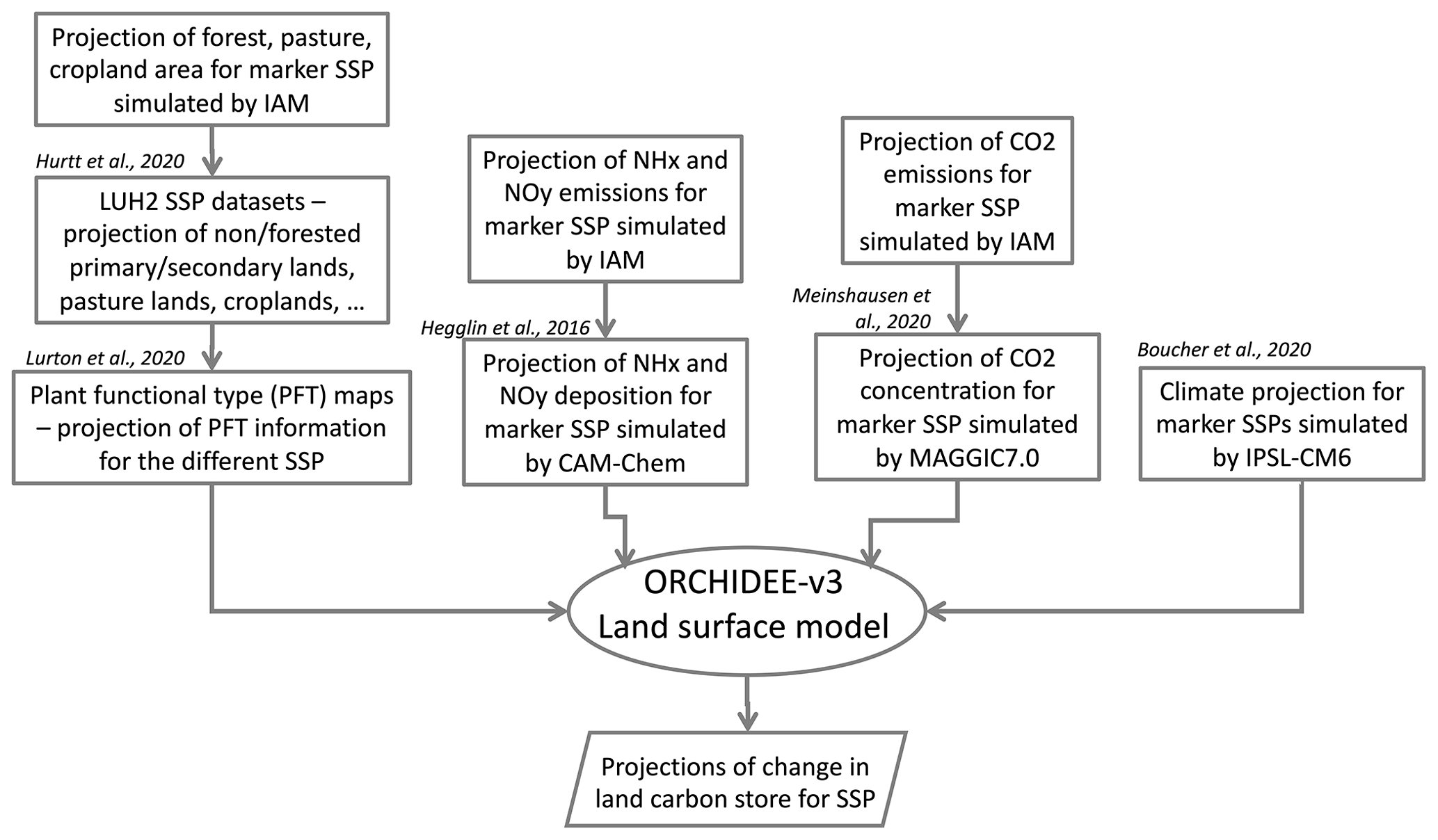
Figure 1 Flowchart of the modelling framework highlighting the different input data (rectangles), the land surface model (ellipsoid) used in this study, and the main output data produced (parallelogram).

2.2 Model input datasets

Inputs related to atmospheric CO₂ concentration ([CO₂]), land use, wood harvest, N fertiliser, and nitrogen deposition are those used for the historical and the different SSP CMIP6-related experiments and stored on input4MIPs nodes (https://aims2.llnl.gov/search/input4MIPs/, last access: 28 August 2024). Land use, wood harvest, and N fertiliser input data are produced by the Land-Use Harmonisation 2 (LUH2) project (Hurtt et al., 2020). Land use information from LUH2 consists of fractions of the grid cell area at 0.25° resolution for cropland (five sub-categories), managed pasture, rangeland, urban, primary forested land, secondary forested land, primary non-forested land, and secondary non-forested land. The procedure needed for translating the original data for land use into the 15 land classes of ORCHIDEE is described in Lurton et al. (2020). In this procedure, information regarding the cropland and pasture areas from LUH2 is preserved, while natural land is split into the different unmanaged land classes of ORCHIDEE using data from the European Space Agency (ESA) Climate Change Initiative (CCI) land cover product for the year 2016 (ESA, 2022). For the period 2015–2100, LUH2 data are based on land use and land management information from the eight different marker scenarios generated by IAMs. Nitrogen deposition fields are produced by the CAM-Chem climate–chemistry model (Hegglin et al., 2016, 2018) with emission data from the different marker scenarios for the period 2015–2100. Climate data used as input to the land-only ORCHIDEE v3 simulations correspond to the IPSL-CM6A-LR model outputs (at a global resolution of 2.5° × 1.27° in longitude and latitude) for the historical period and the different SSP CMIP6 experiments. In this study, ORCHIDEE v3 ran at the same resolution as the climate input data. Figure 1 summarises the modelling framework developed for this study with the different input data used.

2.3 Reference simulations

In order to get C and N vegetation and soil pools to reach equilibrium, we ran a spin-up simulation with the boundary conditions of the year 1850 but recycled climate data for the period 1850–1869 in order to account for an interannual variability. From this equilibrium state, simulations ran for the historical period (1850–2014) and for each of the eight SSP experiments from 2015 to 2100.

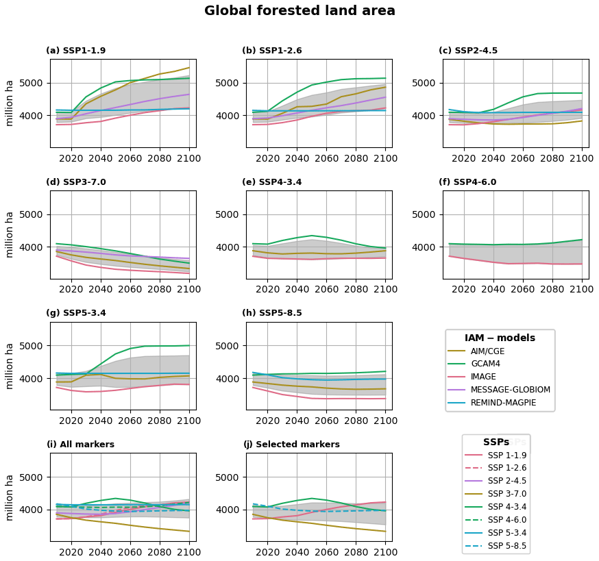
Figure 2 Time evolution (2015–2100) of the global forested land area (Mha) projected by (a–h) different integrated assessment models (IAMs) for different Shared Socioeconomic Pathways (SSPs). (i) All SSP markers and (j) selected SSP markers used in the study. Grey areas represent the time evolution of the mean ± sigma.

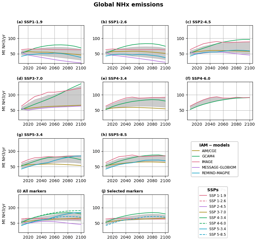
Figure 3 Time evolution (2015–2100) of the global NH_x (NH₃) emissions (Mt (NH₃) yr⁻¹) projected by (a–h) different integrated assessment models (IAMs) for different Shared Socioeconomic Pathways (SSPs). (i) All SSP markers and (j) selected SSP markers used in the study. Grey areas represent the time evolution of the mean ± sigma.

2.4 Land-use and nitrogen-input-related sensitivity simulations

The objective was to investigate the impact on CLCS of the uncertainty associated with land use and nitrogen inputs (i.e. atmospheric N deposition and N fertilisation) for a given SSP  p. Given that all gridded harmonised data for the land use and nitrogen inputs of non-marker scenarios of SSP  p are not available, we used the gridded data (for land use and nitrogen inputs) from marker scenarios of selected alternative SSPs to assess the sensitivity of the projected land carbon store for SSP  p to land use and nitrogen input uncertainties. In other words, we used the inter-selected SSP marker spread as a proxy for the inter-IAM spread regarding the land use and nitrogen input trajectories for any given SSP. This is a strong assumption but supported by the comparison between inter-selected SSP marker trajectories and inter-IAM trajectories for the different SSPs. The comparison has been conducted for the following variables: forested land area (Fig. 2), NH_x emissions (Fig. 3), cropland area (Fig. A1), pasture land area (Fig. A2), and NO_y emissions (Fig. A3). Given that, ultimately, we would like to assess the uncertainty associated with land use and nitrogen inputs from the different IAMs for any SSP, in the following we may use the term “uncertainty” when referring to the different inter-selected SSP marker trajectories although they correspond more to certain trajectories obtained for different assumptions in terms of socioeconomic development and mitigation level.

Due to computing time resources, we limited our sensitivity study to four SSP markers among the eight available, and for each of these four SSPs, we used the land use and nitrogen inputs trajectories of this set of four SSP markers to assess their impacts on CLCS. The inter-selected SSPs were SSP1-1.9, SSP3-7.0, SSP4-3.4, and SSP5-8.5. The inter-selected SSP markers were computed by the integrated assessment models IMAGE, AIM/CGE, GCAM4, and REMIND-MAGPIE, respectively. IAMs are driven by projections of economic growth and population but differ in their representation of socioeconomic-, energy-, and land-related processes. Information on IAM modelling regarding land use allocation and nitrogen emissions can be found in Tables A1 and A2, respectively. We selected these four SSPs because (1) they encompass a large spread of the CO₂ level in 2100 ranging from 394 to 1135 ppm, and (2) the inter-IAM spreads for land use but also N-related input data trajectories from this selection are comparable to those from the eight SSPs.

Based on the IAM output data produced for CMIP6 available on the SSP Database (https://tntcat.iiasa.ac.at/SspD, last access: 28 August 2024), we showed that the inter-selected SSP marker spread of the forested global land area in 2100 is narrower than the inter-IAM spread for six out of eight SSPs (Fig. 2). Similarly, the inter-selected SSP marker spread of the global NH₃ emissions in 2100 is narrower than the inter-IAM spread for seven out of the eight SSPs (Fig. 3). However, for some variables simulated by IAMs, the inter-selected SSP marker spread is significantly larger than the inter-IAM spread for many SSPs. This is particularly the case for NO_y emissions (Fig. A3) for which the inter-selected marker spread is larger than the inter-IAM spread for any of the eight SSPs. Thus, depending on the driving variable considered (forested lands, pasture, or croplands; NH₃ or NO_y emissions) and on the SSP considered, the use of the inter-selected SSP marker spread as a proxy may translate into an upper or lower estimate of the inter-IAM spread. Overall, our assumption of using the land use and N trajectories of the different SSP markers as a surrogate for the trajectories simulated by the different IAMs for each SSP looks reasonable (from the above analysis). The comparison between inter-selected SSP markers and inter-IAM trajectories for the different SSPs is presented at a global scale, but the conclusion that the inter-selected SSP marker spread is comparable to the inter-IAM spread for the different SSPs remains valid at a regional scale (based on the data available in the SSP Database for five aggregated regions, namely “Asia”, “Latin America”, “Reforming economies”, “Middle East and Africa”, and countries from the “Organisation for Economic Co-operation and Development”; not shown).

In addition, using alternative SSP scenarios for a given driving variable (for instance, LUC or nitrogen atmospheric deposition) while keeping the other driving variables from a single SSP may break down the coherency between driving variables as established within each IAM. However, we showed that while NH₃ emissions show a good linear relationship with cropland area for most of the IAMs, the slope of this relationship is significantly different across IAMs (Fig. A4). This indicates that no common and unique relationship exists across IAMs, and thus, using the marker SSP spread for each variable independently of the others is a reasonable assumption.

2.5 Metrics assessing the change in the land carbon store and its sensitivity to different land use and nitrogen inputs

We analysed specifically the projected change in land carbon store (CLCS) for the four selected pathways and its sensitivity to the different land use and N-input marker trajectories from these inter-selected SSPs. To perform this analysis, we ran a set of 16 sensitivity simulations for each of the 4 selected reference simulations where land use and N-related data from the four SSPs are used independently as forcing (4 land use trajectories times 4 N-input trajectories). The trajectories over 2015–2100 of the input data for forested land area, total atmospheric nitrogen deposition, nitrogen fertiliser application, atmospheric [CO₂], and near-surface temperature are shown in Figs. A5–A9, respectively.

We expressed CLCS as a function of climate and atmospheric [CO₂] (CCO2), land use change (LUC), and nitrogen input (NIN) trajectories (CLCS (CCO2, LUC, and NIN)) and quantified the impact of CCO2, LUC, and NIN trajectories on CLCS by computing mean (μ) and standard deviation (σ) metrics based on the following equations:

$$\begin{array}{}\text{(1)}& {\displaystyle }{X}_{\text{CLCS},\text{CCO2}}(j,k)=X\mathit{\left\{}\mathrm{CLCS}\right(i,j,k){\mathit{\}}}_{i=\mathrm{1}\text{-}\mathrm{1.9},\mathrm{3}\text{-}\mathrm{7.0},\mathrm{4}\text{-}\mathrm{3.4},\mathrm{5}\text{-}\mathrm{8.5}},\text{(2)}& {\displaystyle }{X}_{\text{CLCS},\text{LUC}}(i,k)=X\mathit{\left\{}\mathrm{CLCS}\right(i,j,k){\mathit{\}}}_{j=\mathrm{1}\text{-}\mathrm{1.9},\mathrm{3}\text{-}\mathrm{7.0},\mathrm{4}\text{-}\mathrm{3.4},\mathrm{5}\text{-}\mathrm{8.5}},\text{(3)}& {\displaystyle }{X}_{\text{CLCS},\text{NIN}}(i,j)=X\mathit{\left\{}\mathrm{CLCS}\right(i,j,k){\mathit{\}}}_{k=\mathrm{1}\text{-}\mathrm{1.9},\mathrm{3}\text{-}\mathrm{7.0},\mathrm{4}\text{-}\mathrm{3.4},\mathrm{55}\text{-}\mathrm{8.5}},\end{array}$$

where X stands for μ or σ, and the indices  i, j, and k stand for CCO2, LUC, and NIN trajectories, respectively, with each spanning the different SSPs.

From the above generic equations, we can further quantify the mean CLCS and standard deviation associated specifically with different land use (LUC) and different atmospheric N deposition and fertilisation (NIN) trajectories for each of the four selected SSPs (s), $X_{\text{CLCS},\text{LUC}}^s$, and $X_{\text{CLCS},\text{NIN}}^s$, defined as

$$\begin{array}{}\text{(4)}& {\displaystyle }& {\displaystyle }{X}_{\text{CLCS},\text{LUC}}^s=X_{\text{CLCS},\text{LUC}}(i=s,k=s),\text{(5)}& {\displaystyle }& {\displaystyle }\text{and }{X}_{\text{CLCS},\text{NIN}}^s=X_{\text{CLCS},\text{NIN}}(i=s,j=s),\end{array}$$

for s = 1–1.9, 3–7.0, 4–3.4, and 5–8.5.

We also quantified the CLCS and standard deviation associated with land use plus atmospheric N deposition and fertilisation (LUC+NIN), $X_{\text{CLCS},\text{LUC}+\text{NIN}}^s$. It is written as

$$\begin{array}{}\text{(6)}& X_{\text{CLCS},\text{LUC}+\text{NIN}}^s=X\mathit{\left\{}\mathrm{CLCS}\right(i=s,j,k){\mathit{\}}}_{j,k=\mathrm{1}\text{-}\mathrm{1.9},\mathrm{3}\text{-}\mathrm{7.0},\mathrm{4}\text{-}\mathrm{3.4},\mathrm{5}\text{-}\mathrm{8.5}}.\end{array}$$

In order to report on the overall dispersion of CLCS and the contribution from the three drivers (CCO2, LUC, and NIN), we first computed μ and σ, accounting for all drivers, as follows:

$$\begin{array}{}\text{(7)}& X_{\text{CLCS},\text{TOT}}=X\mathit{\left\{}\mathrm{CLCS}\right(i,j,k){\mathit{\}}}_{i,j,k=\mathrm{1}\text{-}\mathrm{1.9},\mathrm{3}\text{-}\mathrm{7.0},\mathrm{4}\text{-}\mathrm{3.4},\mathrm{5}\text{-}\mathrm{8.5}}.\end{array}$$

We then computed the mean standard deviation, ${\stackrel{\mathrm{‾}}{\mathit{\sigma }}}_{\text{CLCS},D}$ in order to quantify the impact on CLCS of each of the three drivers (D being CCO2, LUC, or NIN) irrespective of the combinations of the other two:

$$\begin{array}{}\text{(8)}& {\displaystyle }{\stackrel{\mathrm{‾}}{\mathit{\sigma }}}_{\text{CLCS},\text{CCO2}}=\mathit{\mu }\mathit{\left\{}{\mathit{\sigma }}_{\text{CLCS},\text{CCO2}}\right(j,k){\mathit{\}}}_{j,k=\mathrm{1}\text{-}\mathrm{1.9},\mathrm{3}\text{-}\mathrm{7.0},\mathrm{4}\text{-}\mathrm{3.4},\mathrm{5}\text{-}\mathrm{8.5}},\text{(9)}& {\displaystyle }{\stackrel{\mathrm{‾}}{\mathit{\sigma }}}_{\text{CLCS},\text{LUC}}=\mathit{\mu }\mathit{\left\{}{\mathit{\sigma }}_{\text{CLCS},\text{LUC}}\right(i,k){\mathit{\}}}_{i,k=\mathrm{1}\text{-}\mathrm{1.9},\mathrm{3}\text{-}\mathrm{7.0},\mathrm{4}\text{-}\mathrm{3.4},\mathrm{5}\text{-}\mathrm{8.5}},\text{(10)}& {\displaystyle }{\stackrel{\mathrm{‾}}{\mathit{\sigma }}}_{\text{CLCS},\text{NIN}}=\mathit{\mu }\mathit{\left\{}{\mathit{\sigma }}_{\text{CLCS},\text{NIN}}\right(i,j){\mathit{\}}}_{i,j=\mathrm{1}\text{-}\mathrm{1.9},\mathrm{3}\text{-}\mathrm{7.0},\mathrm{4}\text{-}\mathrm{3.4},\mathrm{5}\text{-}\mathrm{8.5}}.\end{array}$$

Last, we expressed the relative impact on the CLCS spread of each of the three drivers, r_CLCS,D, as

$$\begin{array}{}\text{(11)}& r_{\text{CLCS},D}={\displaystyle \frac{{\stackrel{\mathrm{‾}}{\mathit{\sigma }}}_{\text{CLCS},D}}{{\stackrel{\mathrm{‾}}{\mathit{\sigma }}}_{\text{CLCS},\text{CCO2}}+{\stackrel{\mathrm{‾}}{\mathit{\sigma }}}_{\text{CLCS},\text{LUC}}+{\stackrel{\mathrm{‾}}{\mathit{\sigma }}}_{\text{CLCS},\text{NIN}}}}\times \mathrm{100},\end{array}$$

for D = CCO2, LUC, and NIN.

Table 1 Change in land carbon store (Pg C) for the historical period from 1850 to 2015 (Hist) and for the SSPs from 1850 to 2100 using the marker simulation (Marker) or an ensemble of simulations with different nitrogen deposition trajectories and fertilisation (NIN sensitivity; ${\mathit{\mu }}_{\text{CLCS},\text{NIN}}^s$ ± ${\mathit{\sigma }}_{\text{CLCS},\text{NIN}}^s$, Eq. 5), different land use change trajectories (LUC sensitivity; ${\mathit{\mu }}_{\text{CLCS},\text{LUC}}^s$ ± ${\mathit{\sigma }}_{\text{CLCS},\text{LUC}}^s$, Eq. 4), or different LUC and NIN trajectories (LUC+NIN sensitivity; ${\mathit{\mu }}_{\text{CLCS},\text{LUC}+\text{NIN}}^s$ ± ${\mathit{\sigma }}_{\text{CLCS},\text{LUC}+\text{NIN}}^s$, Eq. 6). Positive values indicate a gain of carbon in the land reservoir.

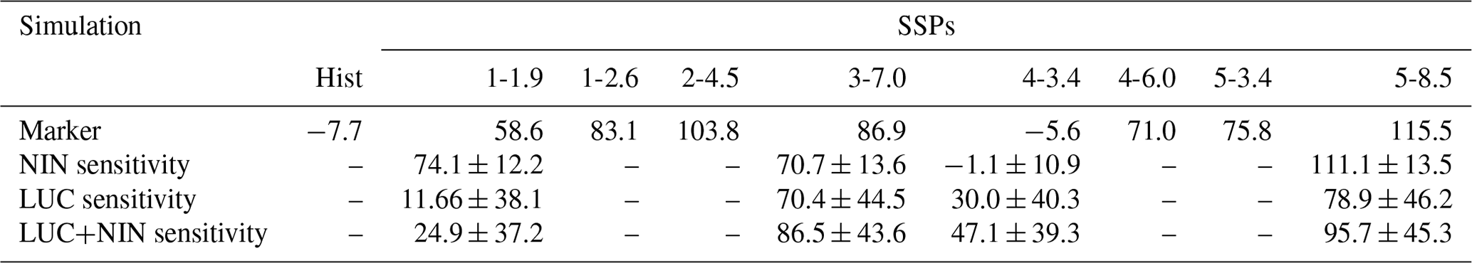
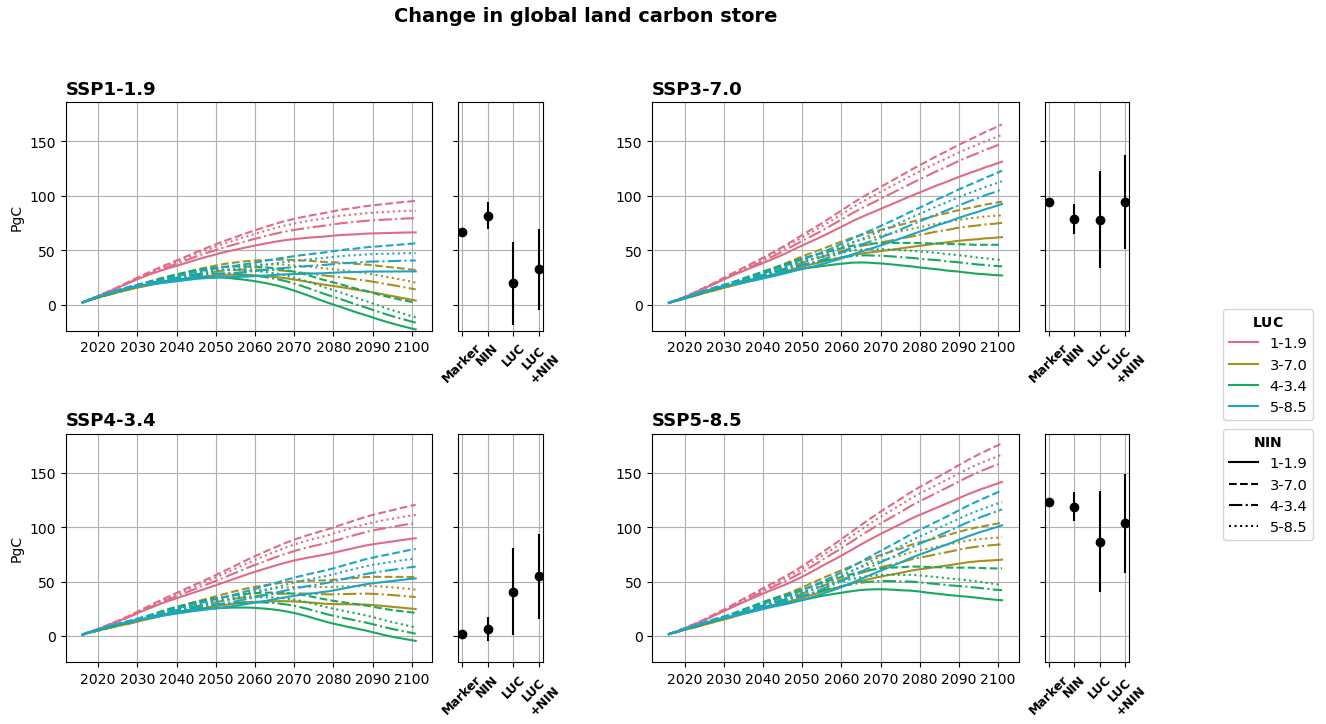
Figure 4 Time evolution over 2015–2100 (left-hand plot of each subpanel) of the global change in land carbon store (CLCS, Pg C) driven by the four atmospheric [CO₂] and associated climate trajectories of the selected SSPs (subpanels SSP1-1.9, SSP3-7.0, SSP4-3.4, and SSP5-8.5) and by different trajectories for land use change (LUC sensitivity; pink, brown, green, and blue lines for SSPs 1-1.9, 3-7.0, 4-3.4, and 5-8.5, respectively) and nitrogen deposition and fertilisation (NIN sensitivity; solid, dashed, dashed–dotted, and dotted lines for SSPs 1-1.9, 3-7.0, 4-3.4, and 5-8.5, respectively). Right-hand plot of each subpanel represents CLCS in 2100 using the marker simulation (Marker) or an ensemble of simulations with different nitrogen deposition and fertilisation trajectories (NIN; ${\mathit{\mu }}_{\text{CLCS},\text{NIN}}^s$ ± ${\mathit{\sigma }}_{\text{CLCS},\text{NIN}}^s$, Eq. 5), different land use change trajectories (LUC; ${\mathit{\mu }}_{\text{CLCS},\text{LUC}}^s$ ± ${\mathit{\sigma }}_{\text{CLCS},\text{LUC}}^s$, Eq. 4), and different LUC and NIN trajectories (LUC+NIN; ${\mathit{\mu }}_{\text{CLCS},\text{LUC}+\text{NIN}}^s$ ± ${\mathit{\sigma }}_{\text{CLCS},\text{LUC}+\text{NIN}}^s$, Eq. 6).

3 Results and discussion

3.1 Change in land carbon store (CLCS) over the historical period and for the different SSP experiments

The change in land carbon store (CLCS) simulated by ORCHIDEE v3 over the historical period (1850–2014) corresponds to a small loss of carbon in the land reservoir of 7.7 Pg C (Table 1, where a negative value corresponds to a source to the atmosphere). This results from a C source due to a land use change larger than the land C sink induced by the increasing [CO₂] and N deposition. Over the period 1850–2100, and depending on the SSP, the CLCS varies between a small source of 5.6 Pg C (SSP4-3.4) and a land sink of 115.5 Pg C (SSP5-8.5). The CLCS simulated by ORCHIDEE v3 is in the low-end range of the values reported by Liddicoat et al. (2021) with an ensemble of nine ESMs (compare Table 1 in this study to Table S3 in Liddicoat et al., 2021). The ORCHIDEE v3 CLCS is very similar to the one simulated by UKESM1-0-LL for the historical period and for any of the seven SSPs studied by this ESM. The CLCS standard deviation induced by considering different N-related trajectories is relatively similar, irrespective of the SSP considered with ${\mathit{\sigma }}_{\text{CLCS},\text{NIN}}^s$ values for the period 1850–2100 varying between 10.9 and 13.6 Pg C, depending on the SSP (Table 1 and Fig. 4). The effect of considering different LUC-related trajectories in the CLCS is more important, with a standard deviation (${\mathit{\sigma }}_{\text{CLCS},\text{LUC}}^s$ for 1850–2100) going from 38.1 Pg C (for SSP1-1.9) to 46.2 Pg C (for SSP5-8.5). Accounting for both sources of uncertainty (LUC and NIN) in CLCS leads to a similar dispersion compared to considering LUC uncertainty only with ${\mathit{\sigma }}_{\text{CLCS},\text{LUC}+\text{NIN}}^s$ varying between 37.2 and 45.3 Pg C, depending on the SSP (Table 1). Expressed as a percentage of the mean CLCS from 2015 to 2100, these values correspond to standard deviations ranging between 43.8 % (for SSP5-8.5) and 114.1 % (for SSP1-1.9) of ${\mathit{\mu }}_{\text{CLCS},\text{LUC}+\text{NIN}}^s$. For SSP1-1.9 with a relative dispersion higher than 100 %, accounting for the spread in LUC and NIN has the capacity to turn CLCS from a gain to a loss of carbon. Although important, these CLCS dispersions induced by the LUC and NIN trajectories are a factor of 2 to 3 less than those associated with the multi-ESM ensemble assessed by Liddicoat et al. (2021) for all four studied SSPs, except SSP1-1.9. Based on the data reported by Liddicoat et al. (2021; Table S3), the CLCS standard deviation of the multi-ESM ensemble over the period 2015–2100 equals 39.6 Pg C (52 % of the multi-ESM ensemble mean), 123.5 Pg C (63 %), 86.9 Pg C (381 %), and 162.3 Pg C (58 %) for SSP1-1.9, SSP3-7.0, SSP4-3.4, and SSP5-8.5, respectively).

As shown in Fig. 4 (right-hand plot of each panel), depending on the LUC and NIN trajectories associated with the marker scenarios, the CLCS from 2015 to 2100 estimated for the marker may be in the very low-end range of the values for all NIN and LUC combinations (SSP4-3.4), in the high-end range (SSP1-1.9), or close to the mean value ${\mathit{\mu }}_{\text{CLCS},\text{LUC}+\text{NIN}}^s$ (SSP3-7.0 and to some extent SSP5-8.5).

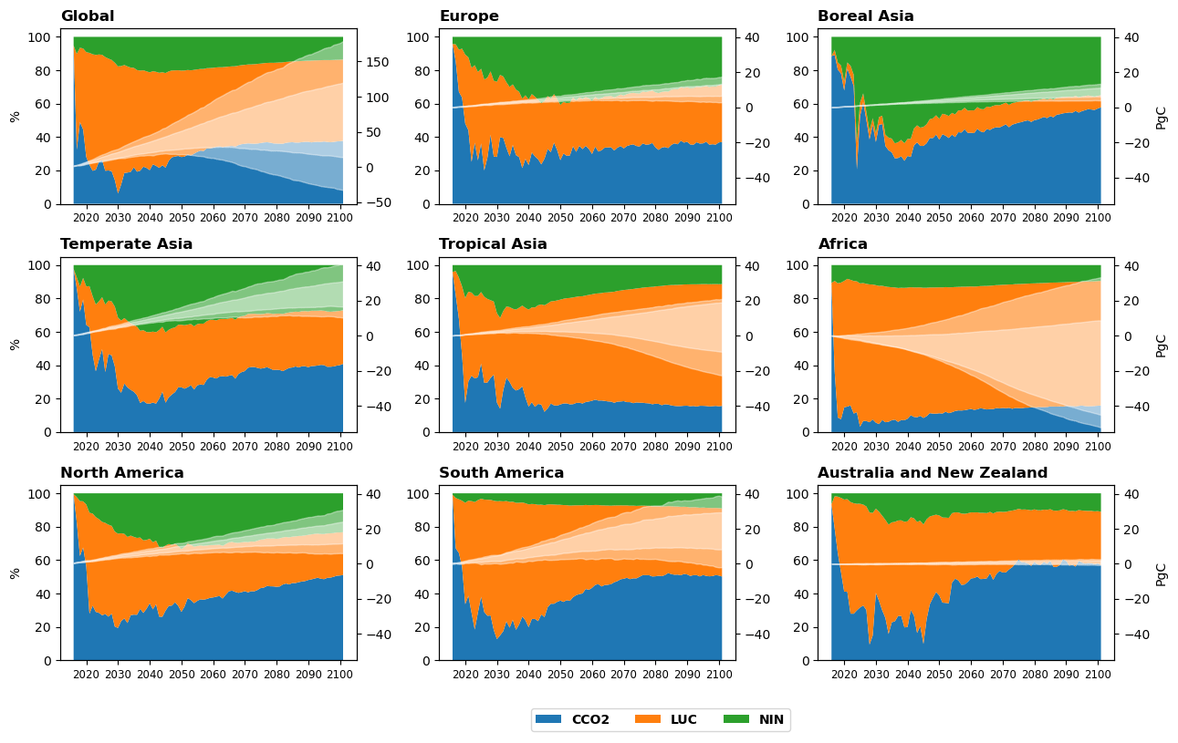
Figure 5 Time evolution (2015–2100) of the change in land carbon store accounting for different atmospheric [CO₂] and associated climate (CCO2), land use change (LUC), and atmospheric N deposition and fertilisation (NIN) trajectories (with the less translucent white area representing μ_CLCS,TOT ± σ_CLCS,TOT; Eq. 7) and the more translucent white area representing the [min;max] of the ensemble of CLCS trajectories (in Pg C; right y axis) and the relative impact on the CLCS dispersion of the three drivers (r_CLCS,D; Eq. 11) (in percentage; left y axis), with D being CCO2 (blue), LUC (orange), or NIN (green).

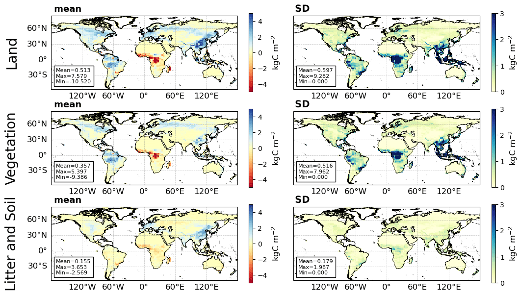
Figure 6 Mean (μ_CLCS,TOT) and standard deviation (σ_CLCS,TOT) of the change by 2100 (relative to 2014) in carbon stored in land (CLCS), vegetation (CVCS), and litter + soil (CSCS) accounting for all the different trajectories regarding atmospheric [CO₂] and associated climate (CCO2), land use change (LUC), and atmospheric N deposition and fertilisation (NIN).

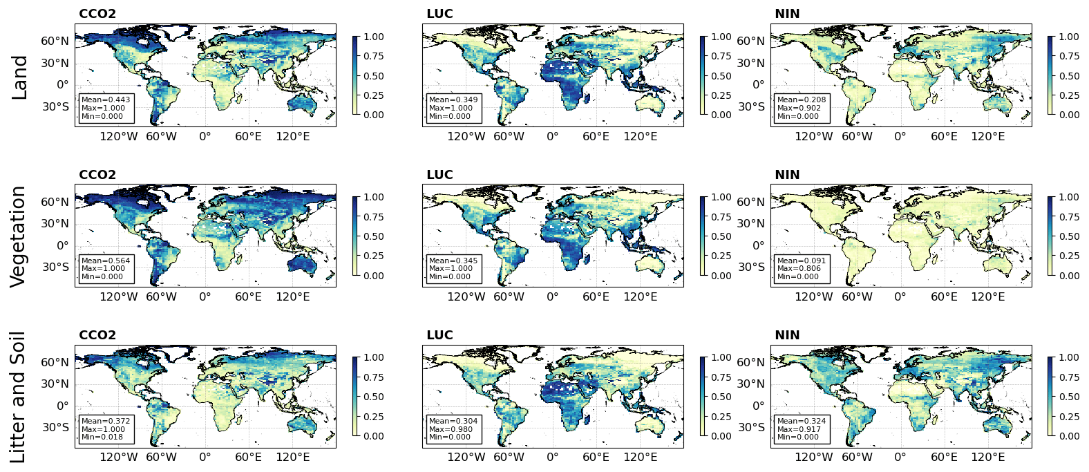
Figure 7 Relative impact (r_CLCS,D (Eq. 11)) of the different trajectories regarding atmospheric [CO₂] and associated climate (CCO2), land use change (LUC), and atmospheric N deposition on the change by 2100 (relatively to 2014) in carbon stored in land (CLCS), vegetation (CVCS), and litter + soil (CSCS).

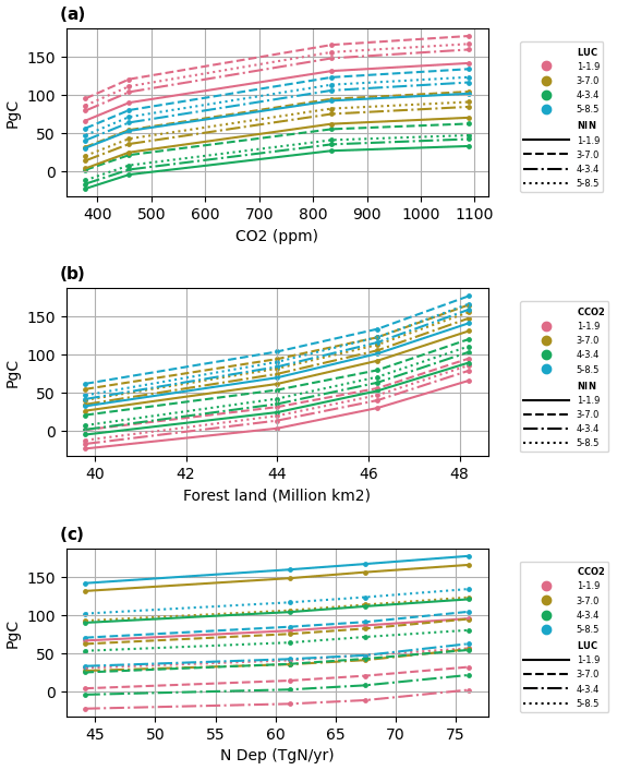
Figure 8 CLCS in 2100 as a function of one of the studied drivers (i.e. a atmospheric CO₂ level for CCO2, b Forested lands for LUC, and c atmospheric N deposition for NIN in 2100) for an ensemble of 16 simulations driven by the different combinations of the other two drivers.

3.2 Spatial and temporal analysis of the CLCS dispersion and its drivers

When accounting for all combinations of NIN, LUC, and CCO2 trajectories, the global CLCS at the end of the 21st century ranges from a source of 33 Pg C to a sink of 179 Pg C (Fig. 5; envelope of the more translucent white areas on the right y axis). The mean change by 2100 (relative to 2014) in carbon stored in land (μ_CLCS,TOT), as well as its standard deviation induced by the different driver trajectories (σ_CLCS,TOT), varies significantly spatially, with a large contribution from Africa and Tropical Asia (and especially tropical forests) to both the mean and standard deviation (Fig. 6). The CLCS spread induced by the different LUC trajectories (σ_CLCS,LUC) is slightly larger than the one related to the CCO2 trajectory (σ_CLCS,CCO2). On average for all combinations of NIN, LUC, and CCO2, the relative impact of LUC on the CLCS spread (r_CLCS,LUC) amounts to 48 % globally at the end of the 21st century, while the r_CLCS,CCO2 value is about 38 % (Fig. 5; coloured areas with a left y axis). The relative impact of NIN on the CLCS spread is one-third less, with a value of r_CLCS,NIN equal to 14 %. The relative impacts of the three drivers on the CLCS spread at the end of the 21st century show contrasting results at regional scale (temporal evolution for the eight global regions in Fig. 5 and spatial distribution in 2100 in Fig. 7). In Africa and Tropical Asia regions, where the strength of the land use change varies significantly from one SSP to another, the relative impact of LUC is far more important than the impact of CCO2 (and NIN), with values of r_CLCS,LUC of ∼ 74 % for both regions (Figs. 5 and 7). As a consequence, the value of r_CLCS,CCO2 in these two regions is less than 20 % by 2100. They are the only two regions for which CLCS shifts significantly from a source to a sink, depending on the LUC trajectories (Fig. 5; envelope of the less translucent white area), with regional ${\mathit{\mu }}_{\text{CLCS},\text{TOT}}\pm {\mathit{\sigma }}_{\text{CLCS},\text{TOT}}$ values of −18 ± 27 Pg C and 5 ± 14 Pg C by 2100 for the “Africa” and the “Tropical Asia” regions, respectively. Due to the strong impact of LUC on CLCS (Figs. 5 and 7) and its large area (Fig. A10), Africa is the region that contributes the most to the overall dispersion of CLCS globally (σ_CLCS,TOT of 27 Pg C for Africa to be compared to σ_CLCS,TOT of 53 Pg C for the globe). For the six other regions where the impact of LUC is less important, CCO2 is the factor that drives the most CLCS dispersion, with r_CLCS,CCO2 values ranging from 37 % (for Europe) to ∼ 57.5 % (for “Boreal Asia” and “Australia and New Zealand” regions). In these regions, the impact of NIN on the CLCS dispersion varies significantly, depending on how the atmospheric N deposition trajectories are contrasted within a region but also on how the terrestrial ecosystems are N-limited regionally. In the “South America” and “Australia and New Zealand regions”, the relative impact of NIN is very small, with r_CLCS,NIN values less than 10 %. In the other four regions, r_CLCS,NIN values are larger than 23 % and up to 35 % for the Boreal Asia region.

The time evolution of the relative impacts of the three drivers on the CLCS dispersion is not uniform over the 21st century (Fig. 5). Globally, r_CLCS,CCO2 decreases over the 2 first decades (2015–2030; from values greater than 50 % down to 7 %) and increases during the following decades with a kind of Michaelis–Menten curve shape. Mirroring the time evolution of the relative impact of CCO2, r_CLCS,NIN, and r_CLCS,LUC increase over the first decades of the 21st century and decrease after 2030 and 2040 for NIN and LUC, respectively. These specific temporal dynamics, which result from the combination of the specific time evolution and time response of the CLCS of the three studied drivers, are obtained globally but also for most of the large regions (e.g. Temperate Asia, North America, and South America). These first-decade dynamics are not analysed in more detail here as they correspond to periods over which the CLCS overall dispersion remains small (see time evolution of ${\mathit{\mu }}_{\text{CLCS},\text{TOT}}\pm {\mathit{\sigma }}_{\text{CLCS},\text{TOT}}$; envelope of the less translucent white area in Fig. 5).

3.3 Change in carbon stored in vegetation and litter and soil pools

Further analysis showed that vegetation (above- and below-ground) is the reservoir contributing the most to CLCS (compared to soil and litter carbon reservoirs; Fig. 6). On average for all combinations of NIN, LUC, and CCO2, the global change in the vegetation carbon store (CVCS) amounts to 47 Pg C at the end of the 21st century (Fig. A11; middle of the less translucent white envelope), while the change in soil and litter carbon store (CSCS) amounts to 21 Pg C (Fig. A13). The overall dispersion of CVCS globally is also much larger than the one of CSCS in 2100 (σ_CVCS,TOT of 52 Pg C; compare to σ_CSCS,TOT of 9 Pg C; see Figs. A11, A13, and 6). Thus, vegetation is also the reservoir which contributes the most to the overall dispersion of CLCS (σ_CLCS,TOT of 53 Pg C for the globe). With carbon in vegetation being mostly stored in trees, forested lands are the main location of CVCS, while grasslands and croplands have only a marginal contribution to CVCS (Fig. A12). On average, the relative impacts of CCO2, LUC, and NIN on the CVCS spread are comparable to those on the CLCS spread with values for r_CVCS,CCO2, r_CVCS,LUC, and r_CVCS,NIN equal to 45 %, 48 %, and 7 %, respectively (Fig. A11). Note, however, that the relative impact of NIN on the CVCS spread is significantly lower than the one on the CLCS spread globally (r_CVCS,NIN of 7 %; compare to r_CLCS,NIN of 14 % for the globe) but also regionally (for instance, in the “Europe” or “Boreal Asia” regions). Compared to the results obtained for the CLCS and CVCS, the relative impacts of CCO2, LUC, and NIN on the CSCS spread are very different (Figs. A13 and 7). NIN is the driver inducing the largest dispersion of CSCS globally (r_CSCS,NIN of 41 %) and in several regions (Europe, Boreal Asia, Temperate Asia, and North America; see Fig. A13). The relative impacts of CCO2 and LUC on the global CSCS dispersion share the remaining percentages equally, with values of 29 % and 30 % for r_CSCS,CCO2 and r_CSCS,LUC, respectively (Fig. A13). The lower relative impact of LUC on the CSCS dispersion compared to the CVCS dispersion can be explained by the fact that land use changes impact the standing biomass more significantly than the modelled soil organic carbon dynamic. For the effect of CCO2, a deeper analysis (not shown) revealed that CCO2 is driving the soil carbon store via two opposite contributions. The soil carbon store increases with the atmospheric [CO₂] increase, while it decreases with soil temperature increase due to higher soil organic decomposition rate. The compensating effects of atmospheric [CO₂] and soil temperature result in limited changes in soil carbon store for the different CCO2 scenarios in which soil temperature varies proportionally to atmospheric [CO₂].

3.4 CLCS as a function of atmospheric CO₂, forested land area, and atmospheric nitrogen deposition

The ensemble of 64 factorial simulations offers the advantage to isolate and quantify the effect of one specific driver among the three considered in this study (CCO2, LUC, and NIN) which are otherwise mixed up in the standard reference SSP simulations. We express CLCS in 2100 (i.e. the total change from 2015 to 2100) as a function of one driver (atmospheric [CO₂] for CCO2, forested lands for LUC, or N atmospheric deposition for NIN in 2100) for the 16 simulations driven by the different combinations of the two other drivers (Fig. 8). The different relationships between CLCS and any of the three drivers are similar, irrespective of the simulations considered, meaning that there are no strong co-varying effects across drivers. Only the CLCS baseline level differs between simulations. The CLCS response curve to [CO₂] shows a saturation effect for the highest CO₂ level (∼ 1100 ppm) driven by the limitation of C assimilated by photosynthesis at high [CO₂]. Based on a simple linear regression, the CLCS response to CO₂ equals 0.1 Pg C ppm⁻¹ (Fig. 8a). Note that this sensitivity cannot be compared to the well-studied land carbon–concentration feedback metric (β_L; Pg C ppm⁻¹) (Arora et al., 2020; Friedlingstein, 2015) since in our study the CLCS response to CO₂ also includes the indirect effect of [CO₂] on the land carbon store via climate change and in particular temperature change.

We also highlight a relationship between the forested land area in 2100 and CLCS in 2100 (Fig. 8b). The forested land area in 2100 is inversely proportional to the deforestation trend (or proportional to the re/afforestation trend) experienced over the 21st century in the different SSPs. As a consequence, the higher forested land area, the higher CLCS. The relationship between CLCS and the forested land area is not strictly linear due to the different regions where the deforestation (or re/afforestation) acts in the SSPs with different ecosystem productivity and vegetation carbon storage (higher storage for tropical ecosystems). However, on average, based on a linear regression, the CLCS response to the forested lands equals 13.85 Pg C (Mkm² of forested lands)⁻¹ (Fig. 8b). Last, CLCS shows a nearly linear relationship with the global mean atmospheric N deposition rate in 2100 (Fig. 8c). The 2100 rate is used here as an indicator of the load of atmospheric N deposited on land over the 21st century and its fertilising effect on terrestrial ecosystems. This results in a CLCS response to the N deposition of 1 $\mathrm{Pg}\mathrm{C}(\mathrm{Tg}\mathrm{N}{\mathrm{yr}}^{-\mathrm{1}}{)}^{-\mathrm{1}}$.

3.5 Comparison with other studies and a path for future research

To our knowledge, little attention has been paid to the co-effects of atmospheric [CO₂], atmospheric nitrogen deposition, and land use change on the change in the land carbon store in the CMIP6 framework and how these drivers interplay at global and regional scales. A 1pctCO2 experiment was part of the DECK ensemble (Eyring et al., 2016) in order to analyse the effects of a 1 % yr⁻¹ increase in atmospheric [CO₂] on the radiative (RAD) and carbon cycle (BGC) components with pre-industrial atmospheric N deposition. In addition to the 1pctCO2 experiment, two experiments (namely 1pctCO2Ndep and 1pctCO2Ndep-bgc) were planned in the Coupled Climate–Carbon Cycle Model Intercomparison Project (Jones et al., 2016) with time-increasing atmospheric N deposition with the objective of quantifying the co-effects of atmospheric CO₂ and N deposition increases. Unfortunately, only three modelling groups performed these two additional experiments, and no study has made use of them so far. In the Land Use Model Intercomparison Project (Lawrence et al., 2016), the two experiments ssp370-ssp126Lu and ssp126-ssp370Lu, based on the ScenarioMIP ssp370 and ssp126 experiments but swapping their land use datasets (Hurtt et al., 2020), aim at quantifying the specific contribution from land use change to the climate and carbon cycle over the 21st century. With this set of 2 × 2 experiments, Ito et al. (2019) quantified the impact of land use change on the total soil carbon stock (cSoil) simulated by seven ESMs. Although limited to only two contrasting land use trajectories, they reported a large intermodel spread with a change in cSoil in 2100 between pair experiments (which differ only by their land use trajectories) varying between −14 and +28 Pg C, depending on the ESM. The large intermodel spread regarding changes in the land carbon store has also been reported in many studies such as the one of Liddicoat et al. (2021), based on the CMIP6 historical and SSPs experiments, or the one of O'Sullivan et al. (2022), based on the ensemble of TRENDY land models over the last 6 decades. In this latter study, 18 land surface models were used to assess the changes in carbon stored in vegetation and soil due to change in CO₂ and nitrogen deposition, climate, and land use. ORCHIDEE v3 was one of these models and showed results very similar to those obtained with the multimodel ensemble means; this gives us confidence in how relevant the results of the present study are. Nevertheless, there is a need to perform the multi-sensitivity analysis we proposed in this paper with an extended ensemble of models in order to evaluate the robustness of our conclusions with other models that have different representations of the key C-related ecosystem processes.

4 Summary and conclusions

Our study aimed to quantify the impacts of the land-use- and nitrogen-input-related IAM uncertainties on the change in land carbon store as simulated by the land component of an ESM forced by climate projections. In the absence of harmonised and downscaled gridded information for the IAMs, other than the marker one of each SSP, we used the land use and nitrogen trajectories of the different SSP markers as a surrogate of the trajectories simulated by the different IAMs for each SSP. We showed that the spread of the simulated change in the global land carbon store induced by the different land use trajectories across SSPs is slightly larger than the one associated with the different atmospheric [CO₂] trajectories. Globally, the uncertainty associated with N inputs (mostly N depositions which originate from the N emissions) is responsible for a spread in the change in the land carbon store that is lower by a factor of 3 than the one driven by atmospheric [CO₂] or land use changes. The relative impact of these different uncertainties showed contrasting responses regionally. In regions with very contrasting land use trajectories across SSPs, such as Africa, the spread in the change in land carbon store is mainly driven by land use change. In contrast, in regions where land use trajectories are more similar across SSPs, the impact of the nitrogen-deposition-related uncertainty on the change in land carbon store may be almost as large as the one induced by the uncertainty in atmospheric CO₂ and land use changes. In addition, we separated the change in land carbon store between a change in the vegetation reservoir and a change in the soil and litter C reservoirs, indicating a much larger contribution from the vegetation. Although we showed that the inter-marker spread and the inter-IAM spread for a given SSP were of the same order for the land use trajectories but also for the global trajectories of N emissions, the two spreads are not strictly similar for each diagnostic variable by the IAMs or for each SSP. In this respect, there is a need to deliver harmonised and downscaled information about land use changes, N emissions, and N atmospheric deposition trajectories simulated by all IAMs for each SSP and not only by the marker IAMs. Performing sensitivity ESM or land-only experiments with these extra datasets is the only way to accurately assess the specific IAM-related uncertainty impacts on the carbon cycle and the climate system. While many GHG mitigation strategies rely more and more on land-based solutions, this calls for facilitating the communication and evaluation between IAM and ESM modelling frameworks. Making additional IAM scenarios available to be used in the next CMIP exercise should contribute to this objective. In addition, given the large impact of the land use change differences between IAMs (for a given SSP) and the significant impact (although lower) of N inputs, we also recommend that the IAM community provides more information on the uncertainties associated with these drivers. For instance, it would be informative to obtain quantitative information on the uncertainty associated with these variables, with a high- and a low-range trajectory for each driver, and whether these uncertainties stand from structural or parametric IAM uncertainties. Information on the level of correlation between the uncertainty associated with each driver (land use and N inputs) would also help to propagate them in the state variables of LSM and ESM simulations.

Appendix A

Table A1 General and land-use-related information for the four integrated assessment models specifically used in this study (adapted from Popp et al., 2017, and Rao et al., 2017).

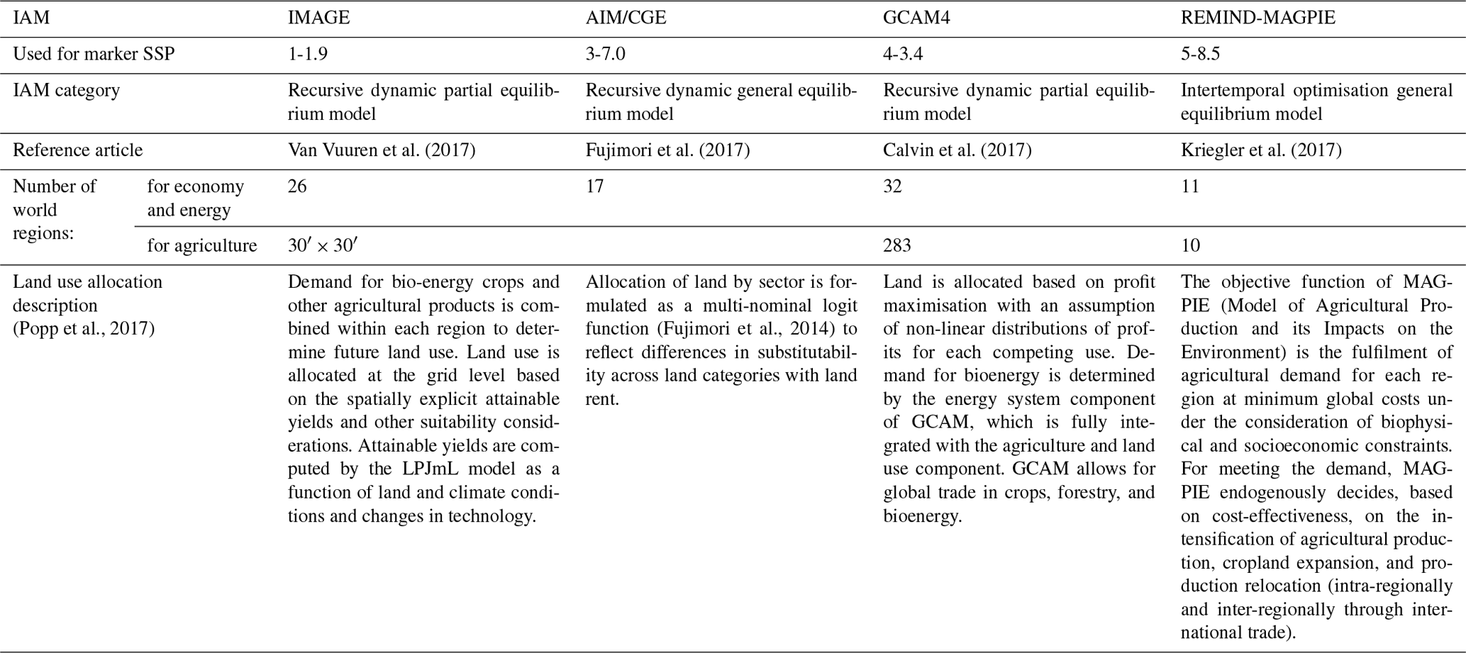
Table A2 Information on NO_x and NH₃ emission modelling for the four integrated assessment models specifically used in this study, with details about the categories and subcategories emitting NO_x/NH₃, the modelling approach used (EF, GE, GM, or EX), and the activity data used (adapted from Rao et al., 2017). EF, GE, GM, and EX stand for “Regional emission factor applied to the specified activity level”, “Grid-specific emission calculated from gridded activity level and (regional) emission factor”, “Gridded, model-based emission (statistical or process-based model)”, and “Exogenous trajectory developed and implemented in model”, respectively. Note that GDP stands for gross domestic product.

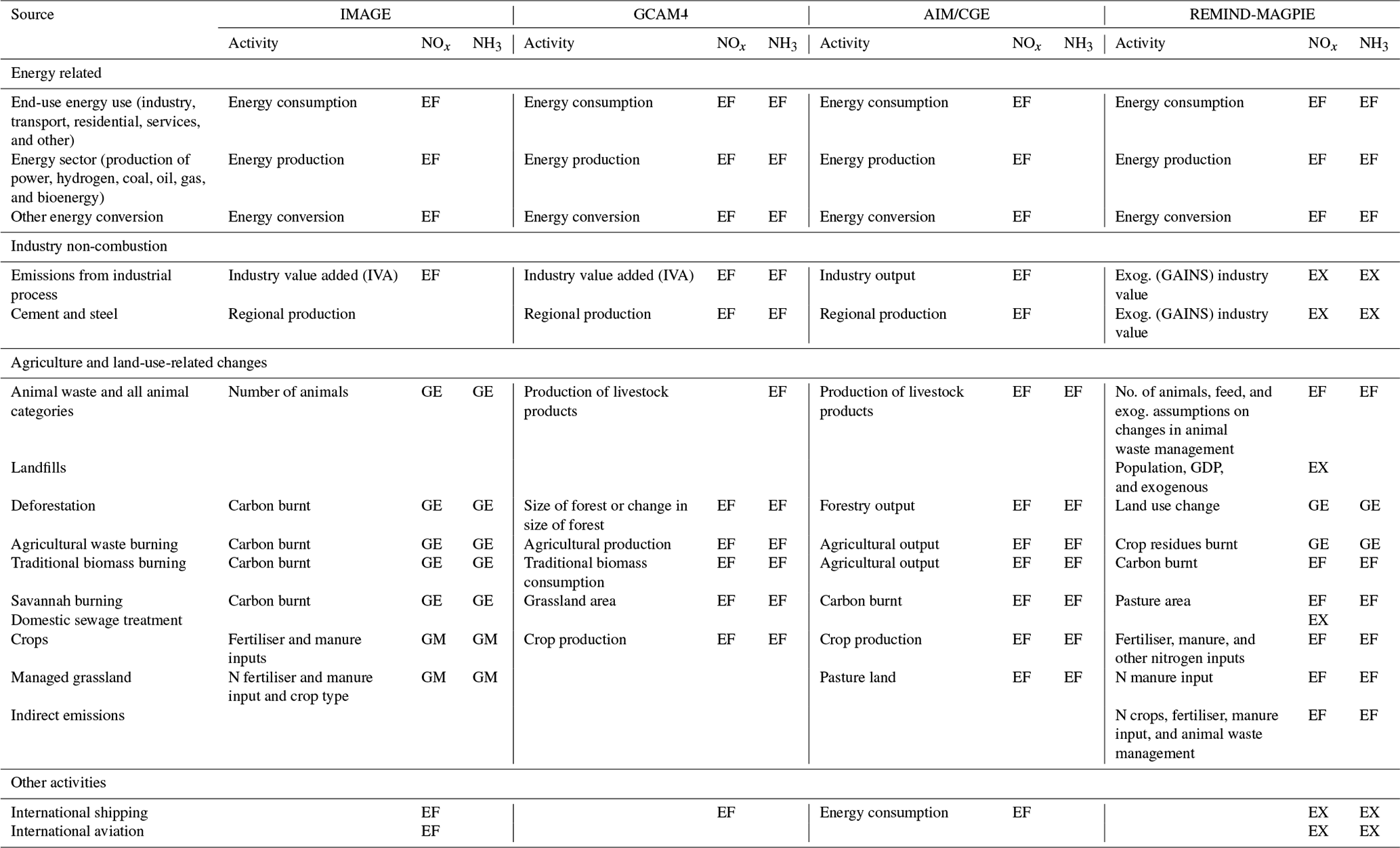
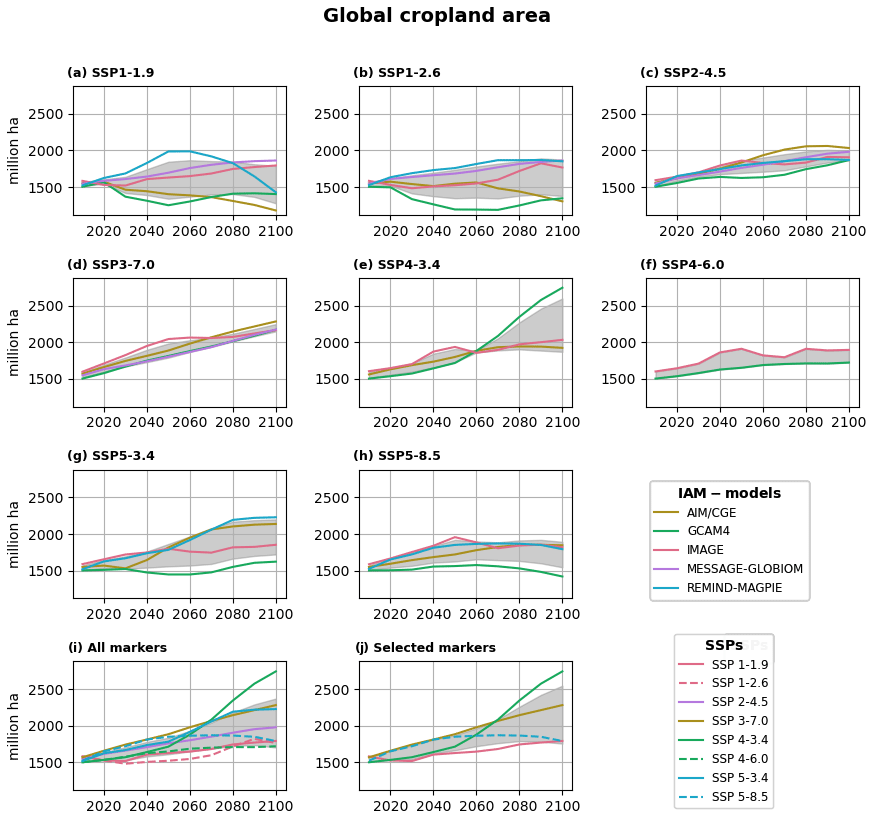
Figure A1 Time evolution (2015–2100) of the global cropland area (Mha) projected by (a–h) different integrated assessment models (IAMs) for different Shared Socioeconomic Pathways (SSPs). (i) All SSP markers and (j) selected SSP markers used in the study. Grey areas represent the time evolution of the mean ± sigma. Data are from https://tntcat.iiasa.ac.at/SspDb (last access: 28 August 2024).

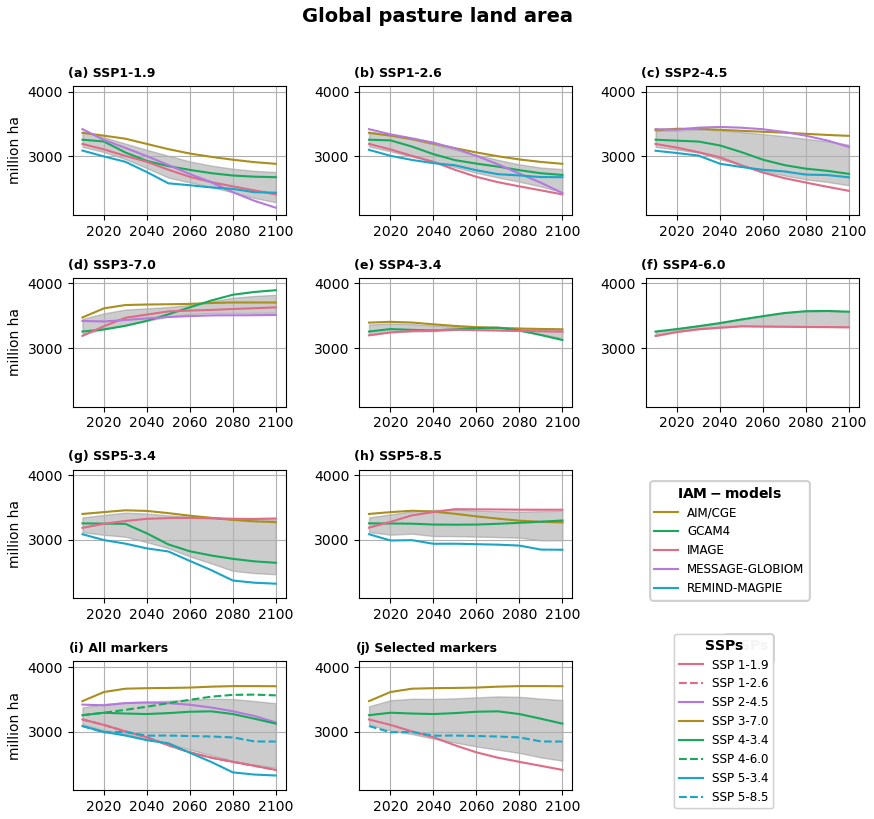
Figure A2 Time evolution (2015–2100) of the global pasture land area (Mha) projected by (a–h) different integrated assessment models (IAMs) for different Shared Socioeconomic Pathways (SSPs). (i) All SSP markers and (j) selected SSP markers used in the study. Grey areas represent the time evolution of the mean ± sigma. Data are from https://tntcat.iiasa.ac.at/SspDb (last access: 28 August 2024)

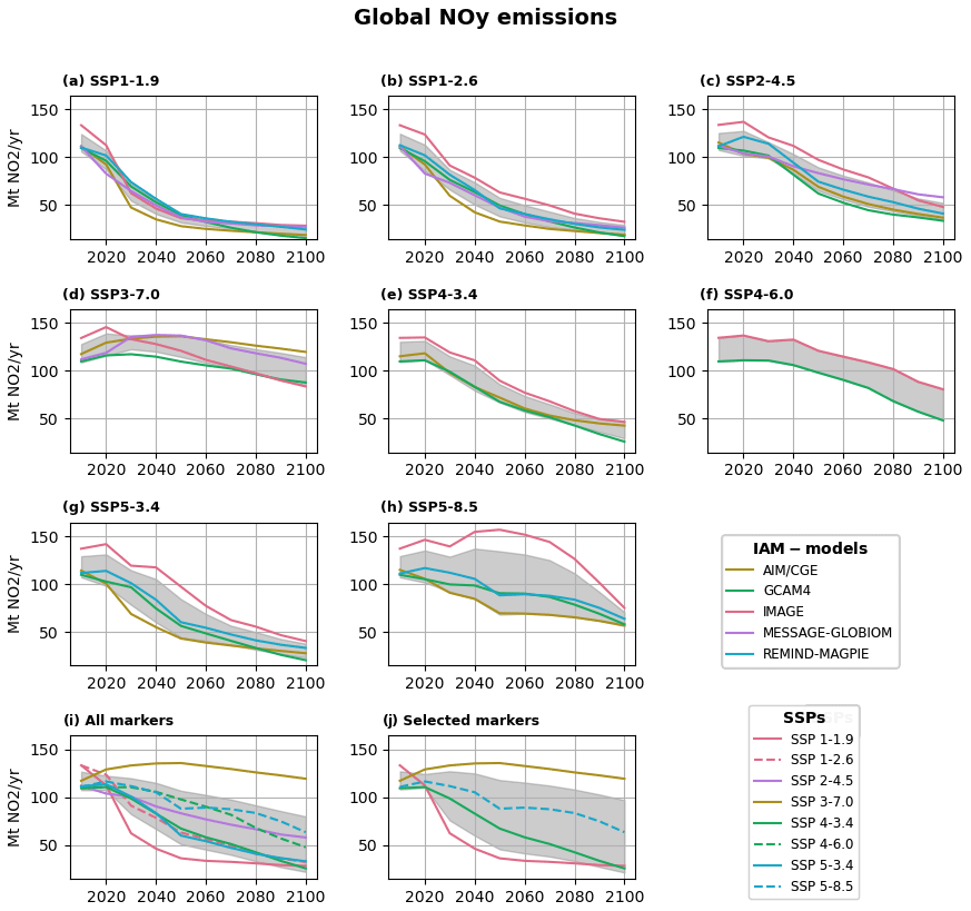
Figure A3 Time evolution (2015–2100) of the global NO_y (NO₂) emissions (Mt (NO₂) yr⁻¹) projected by (a–h) different integrated assessment models (IAMs) for different Shared Socioeconomic Pathways (SSPs). (i) All SSP markers and (j) selected SSP markers used in the study. Grey areas represent the time evolution of the mean ± sigma. Data are from https://tntcat.iiasa.ac.at/SspDb (last access: 28 August 2024).

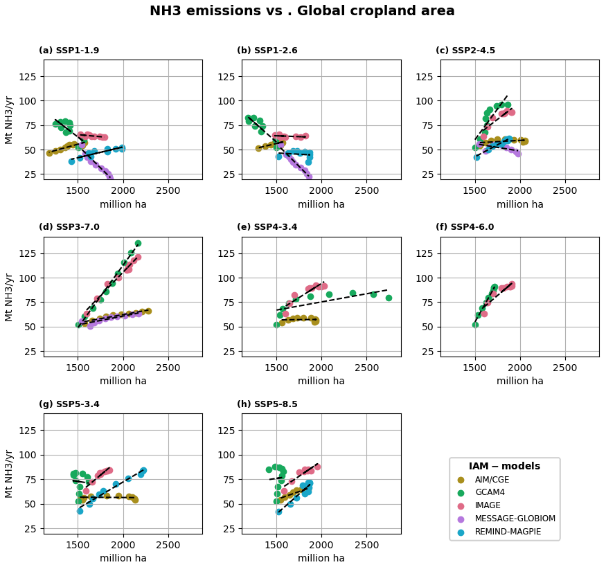
Figure A4 NH₃ emissions (Mt (NH₃) yr⁻¹) as a function of global cropland area (millions of ha) projected by different integrated assessment models (IAMs) for different Shared Socioeconomic Pathways. Data are from https://tntcat.iiasa.ac.at/SspDb (last access: 28 August 2024).

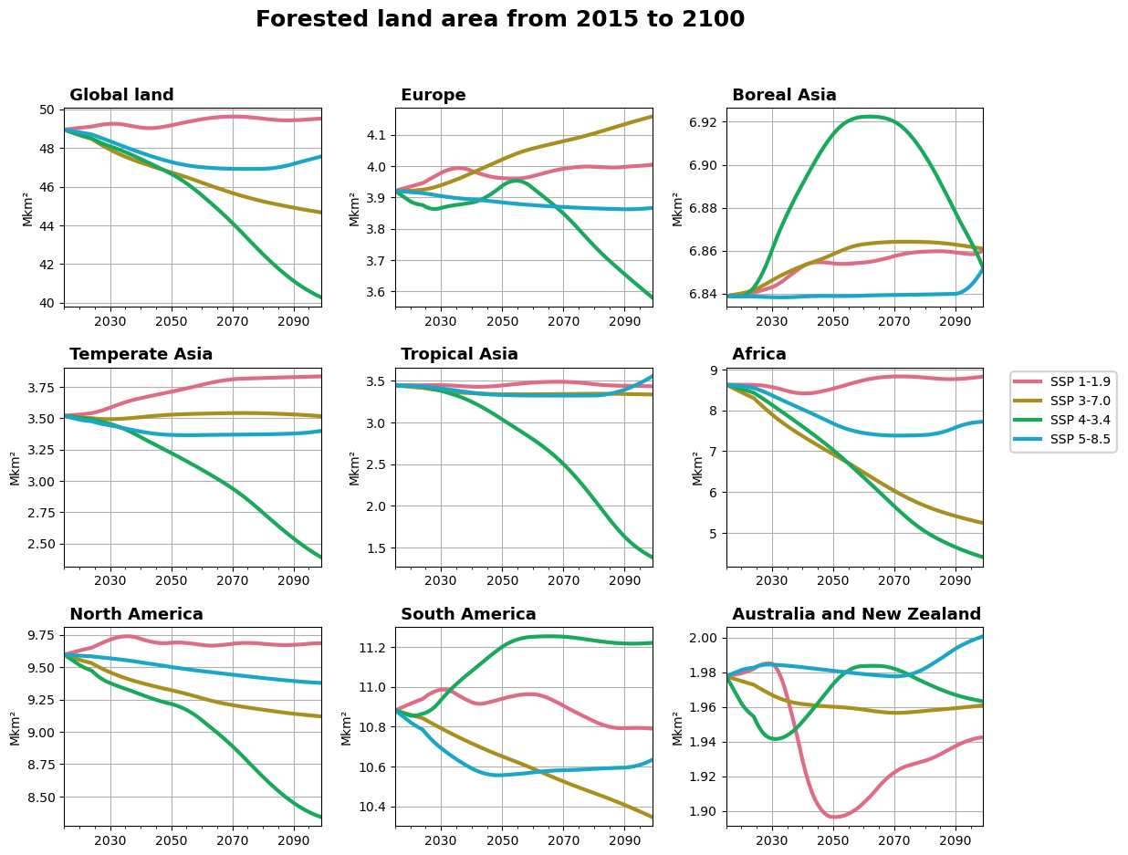
Figure A5 Forested land area projected for SSPs 1-1.9, 3-7.0, 4-3.4, and 5-8.5 over 2015–2100 and used as forcing of the ORCHIDEE v3 model used in this study. Data are from the LUH2 project (Hurtt et al., 2020).

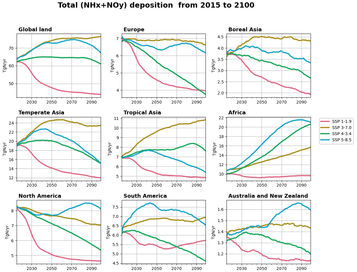
Figure A6 Total atmospheric nitrogen deposition projected for SSPs 1-1.9, 3-7.0, 4-3.4, and 5-8.5 over 2015–2100 and used as forcing of the ORCHIDEE v3 model used in this study. Data are from Hegglin et al. (2016, 2018).

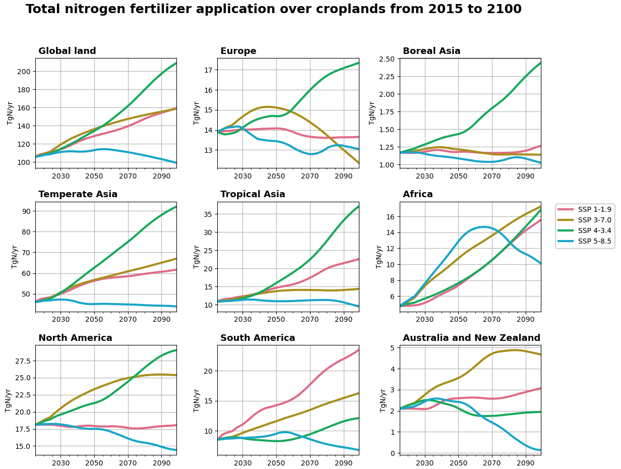
Figure A7 Nitrogen fertiliser application projected for SSPs 1-1.9, 3-7.0, 4-3.4, and 5-8.5 over 2015–2100 and used as forcing of the ORCHIDEE v3 model used in this study. Data are from the LUH2 project (Hurtt et al., 2020).

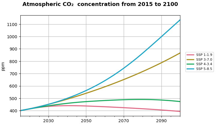
Figure A8 Atmospheric CO₂ concentrations projected for SSPs 1-1.9, 3-7.0, 4-3.4, and 5-8.5 over 2015–2100 and used as forcing of the ORCHIDEE v3 model used in this study.

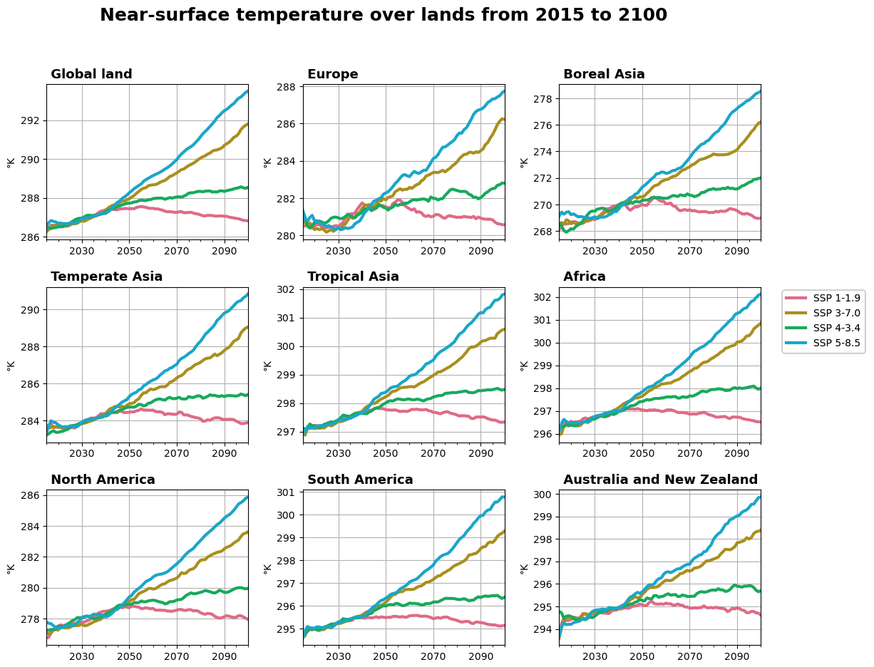
Figure A9 Near-surface temperature projected by the IPSL-CM6 ESM for SSPs 1-1.9, 3-7.0, 4-3.4, and 5-8.5 over 2015–2100 and used as forcing of the ORCHIDEE v3 model used in this study. Data are from IPSL-CM6 (Boucher et al., 2020).

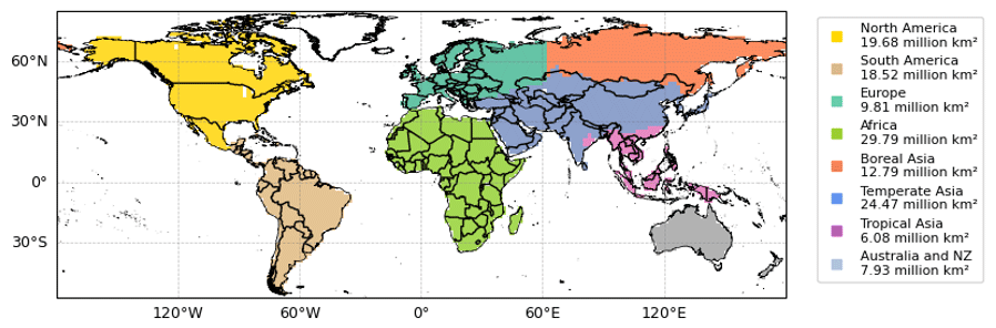
Figure A10 Spatial distribution and size area of the eight regions used in the study.

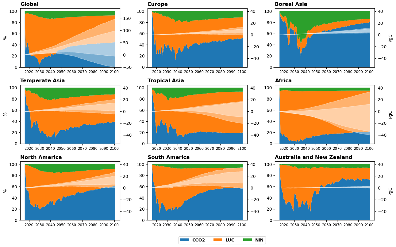
Figure A11 Time evolution (2015–2100) of the change in the vegetation carbon store (CVCS) accounting for different atmospheric [CO₂] and associated climate (CCO2), land use change (LUC), and atmospheric N deposition and fertilisation (NIN) trajectories (with the less translucent white area representing μ_CVCS,TOT ± σ_CVCS,TOT and the more translucent white area representing the $[min;max]$ of the ensemble of CVCS trajectories; in Pg C; right y axis) and the relative impact on the CVCS dispersion of the three drivers (r_CVCS,D; in percentage; left y axis) with D being CCO2 (blue), LUC (orange), or NIN (green).

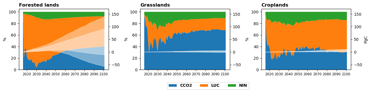
Figure A12 Time evolution (2015–2100) of the global change in the vegetation carbon store (CVCS) for tree, grass, and crop cover accounting for different atmospheric [CO₂] and associated climate (CCO2) land use change (LUC) and atmospheric N deposition and fertilisation (NIN) trajectories (with the less translucent white area representing μ_CVCS,TOT ± σ_CVCS,TOT and the more translucent white area representing the $[min;max]$ of the ensemble of CVCS trajectories; in Pg C; right y axis) and the relative impact on the CVCS dispersion of the three drivers (r_CVCS,D; in percentage; left y axis) with D being CCO2 (blue), LUC (orange), or NIN (green).

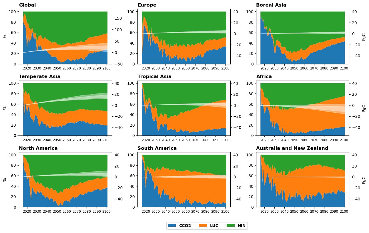
Figure A13 Time evolution (2015–2100) of the change in the litter and soil carbon store (CSCS) accounting for uncertainty in atmospheric [CO₂] and associated climate (CCO2) land use change (LUC) and atmospheric N deposition and fertilisation (NIN) trajectories (with the less translucent white area representing μ_CSCS,TOT ± σ_CSCS,TOT and the more translucent white area representing the $[min;max]$ of the ensemble of CSCS trajectories; in Pg C; right y axis) and the relative impact on the CSCS dispersion of the three drivers (r_CSCS,D; in percentage; left y axis) with D being CCO2 (blue), LUC (orange), or NIN (green).