the Creative Commons Attribution 4.0 License.
the Creative Commons Attribution 4.0 License.
 | 26 Aug 2024
Storylines of summer Arctic climate change constrained by Barents–Kara seas and Arctic tropospheric warming for climate risk assessment
Ryan S. Williams
Gareth Marshall
Andrew Orr
Lise Seland Graff
Dörthe Handorf
Alexey Karpechko
Raphael Köhler
René R. Wijngaard
Nadine Johnston
Hanna Lee
Lars Nieradzik
Priscilla A. Mooney
While climate models broadly agree on the changes expected to occur over the Arctic with global warming on a pan-Arctic scale (i.e. polar amplification, sea ice loss, and increased precipitation), the magnitude and patterns of these changes at regional and local scales remain uncertain. This limits the usability of climate model projections for risk assessments and their impact on human activities or ecosystems (e.g. fires and permafrost thawing). Whereas any single or ensemble mean projection may be of limited use to stakeholders, recent studies have shown the value of the storyline approach in providing a comprehensive and tractable set of climate projections that can be used to evaluate changes in environmental or societal risks associated with global warming.
Here, we apply the storyline approach to a large ensemble of the Coupled Model Intercomparison Project Phase 6 (CMIP6) models with the aim of distilling the wide spread in model predictions into four physically plausible outcomes of Arctic summertime climate change. This is made possible by leveraging strong covariability in the climate system associated with well-known but poorly constrained teleconnections and local processes; specifically, we find that differences in Barents–Kara sea warming and lower-tropospheric warming over polar regions among CMIP6 models explain most of the inter-model variability in pan-Arctic surface summer climate response to global warming. Based on this novel finding, we compare regional disparities in climate change across the four storylines. Our storyline analysis highlights the fact that for a given amount of global warming, certain climate risks can be intensified, while others may be lessened, relative to a “middle-of-the-road” ensemble mean projection. We find this to be particularly relevant when comparing climate change over terrestrial and marine areas of the Arctic which can show substantial differences in their sensitivity to global warming. We conclude by discussing the potential implications of our findings for modelling climate change impacts on ecosystems and human activities.
- Article
(9924 KB) - Full-text XML
- BibTeX
- EndNote


Since the late 20th century, the surface of the Arctic has warmed 2 to 4 times faster than the global average, which is referred to as Arctic amplification (hereinafter AA; e.g. Jansen et al., 2020; England et al., 2021; Rantanen et al., 2022). This warming amplification of the near-surface and troposphere is caused by a number of feedbacks involving oceanic, cryospheric, and atmospheric processes (Previdi et al., 2021). Sea ice cover loss in the Arctic Ocean explains the bulk of the near-surface warming, especially over marine areas and coastal terrestrial regions, due to its impact on surface energy fluxes and upper-ocean warming (e.g. Screen and Simmonds, 2010; Dai et al., 2019; Jenkins and Dai, 2021). Sea ice loss and sea surface warming have been singularly strong in the Barents–Kara seas, which have been identified as a warming hotspot (Lind et al., 2018) and a mediator of climate change between the North Atlantic and central Arctic oceans (Smedsrud et al., 2013). AA is also tied to tropospheric warming which is influenced to a greater extent by atmospheric dynamical feedback, such as temperature feedbacks (Pithan and Mauritsen, 2014) and poleward atmospheric energy transport feedback (e.g. Merlis and Henry, 2018). Overall, the combined influence of oceanic, cryospheric, and atmospheric processes render Arctic climate change and its surface warming amplification especially complex to predict.
AA has resulted in extensive loss of land ice, snow cover, and thawing of the permafrost over the Arctic region (e.g. Callaghan et al., 2011; van den Broeke et al., 2016; Chadburn et al., 2017; The IMBIE Team, 2020). These profound changes to the Arctic climate system have been linked to increases in a range of societal and ecological risks (Yumashev et al., 2019). For example, the past few decades have shown an increase in the frequency and intensity of wildfires in many Arctic regions, such as North America's boreal forests (Masrur et al., 2018; McCarty et al., 2021), which has been attributed to unusually warm and dry spring and summer weather conditions (Krikken et al., 2021), as well as increased lightning activity (Veraverbeke et al., 2017). Likewise, the accelerated thawing of permafrost over large swathes of the terrestrial Arctic poses significant challenges for the integrity of local infrastructure, such as roads and buildings (Hjort et al., 2022). Impacts of climate change in the Arctic also extend to marine areas. For example, while increased sunlight in the photic zone from sea ice loss and warmer sea surface temperature may have boosted marine primary production in the Arctic oceans in past decades (Arrigo and Van Dijken, 2015), evidence suggests that this is primarily benefiting species typically found at lower latitudes at the expense of native Arctic species (Ingvaldsen et al., 2021). Changes to the Arctic climate system have also been suggested to have caused an increase in the frequency and intensity of certain extreme weather over the Northern Hemisphere midlatitudes (Cohen et al., 2014), although the mechanisms of action and broader importance of such polar-to-midlatitude teleconnections remain controversial (Vavrus, 2018). The loss of glaciers/land ice from Greenland, through both increased surface meltwater runoff and increased glacier flow/dynamic ice loss, has been a major contributor to increased global sea level rise (e.g. Rignot et al., 2011; The IMBIE team, 2020).
Assessing the many impacts of climate change in the Arctic requires a strong understanding of the physical state of the atmosphere, ocean, and sea ice and how it will respond to climate change. This, however, has been hampered by future climate projections from global coupled climate models showing a wide range of possible outcomes (Overland et al., 2019; Notz and SIMIP Community, 2020; McCrystall et al., 2021; Arias et al., 2021) which stems from uncertainties in possible future greenhouse gas emission scenarios, an incomplete understanding of key climate processes and their imperfect representation in models (model uncertainty), and natural (internal) variability within the climate system (Hawkins and Sutton, 2009). This lack of certainty poses considerable challenges for the planning and implementation of effective mitigation strategies by stakeholders impacted locally or remotely by Arctic climate change. The issue is often poorly addressed through the use of either a single-model or multi-model mean climate projection (Shepherd et al., 2018).
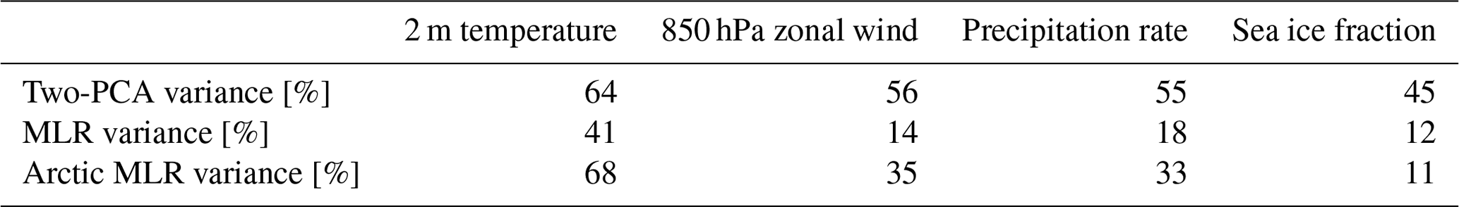
Table 1Explained variance for 2 m temperature, sea ice fraction, and precipitation rate over the Arctic (poleward of 55° N) and 850 hPa zonal wind over the Northern Hemisphere high-latitude regions (poleward of 40° N) in the extended boreal summer (May to October), expressed as a percentage of the total variance across model projections. Each column shows a target variable. The first row is the amount of variance explained by the first two modes of a PCA on the respective target variable, which is the maximum amount of variance that could be explained by a two-predictor MLR. The second row is the amount of variance explained by our two-predictor MLR (Eq. 1a) with ArcAmp and BKWarm as predictors. The third row is the amount of variance explained by our two-predictor MLR averaged over the Arctic (2 m temperature, precipitation rate, and sea ice fraction) and NH high-latitude regions (850 hPa zonal wind).
The storyline approach overcomes the limitations of the above approaches by identifying and describing physically plausible and self-consistent pathways that are representative of future climate change and which may be more helpful to develop mitigation strategies (Shepherd et al., 2018). Storylines express the response of the Arctic climate to global warming that is conditional on a range of environmental conditions being realised. They are based on a methodology recently developed for studying the impact of climate change in other areas, primarily in the midlatitudes, e.g. western and central Europe (Zappa and Shepherd, 2017; hereafter ZS17) or Southern Hemisphere midlatitude regions (Mindlin et al., 2020; hereafter M20). In this study, we posit that a substantial fraction of the variability in the surface climate response to global warming in the Arctic is associated with the warming of the Barents–Kara seas and the warming of the Arctic lower troposphere. This is borne out of Barents–Kara sea warming and the lower-tropospheric warming being strongly influenced by climate variability at lower latitudes but also being key players in driving surface warming in the Arctic. The Barents–Kara seas, while being sensitive to changes in the Atlantic storm track (Jung et al., 2017) and the tropics (Warner et al., 2020), have long been recognised as key modulators of climate variability in Earth's northernmost regions (Li et al., 2021; Peings et al., 2023). Likewise, the warming of the Arctic lower troposphere, which is sensitive to changes in poleward atmospheric heat transport from lower latitudes (Russotto and Biasutti, 2020), strongly influences the near-surface climate through its impact on the boundary layer stability and surface radiative forcing (e.g. Previdi et al., 2020).
Using a range of possible scenarios for the Barents–Kara seas and Arctic lower-tropospheric warming that emerge from climate model simulations, we devise storylines of future climate change for Arctic regions. Specifically, we compare the climate of the last 30 years of the 21st century (2070–2099) projected in a high-end global warming scenario (corresponding to an 8.5 W m−2 additional increase in radiative forcing by 2100 relative to the preindustrial period; see the Shared Socioeconomic Pathways 5-8.5, SSP5-8.5; see O'Neill et al., 2016, and Meinshausen et al., 2020), with the last 30 years of the historical experiment (1985–2014). SSP5-8.5 represents the upper boundary of the range of scenarios described in the Scenario Model Intercomparison Project (ScenarioMIP) and is useful to obtain the strongest possible response to climate change within the framework of the Coupled Model Intercomparison Project Phase 6 (CMIP6); this ensures that the impact of internal climate variabilities is minimised in our study. We focus on the summer season due to its relevance for societal and ecological impacts at high latitudes that peak in the warm part of the year, such as, among others, high-latitude fires, trans-Arctic shipping, and marine primary production. After describing the dataset and methodology used for our storyline analysis in Sect. 2, we describe in Sect. 3 how our Arctic storylines differ from the multi-model ensemble mean response as established by four target variables we identified as being most relevant for studying climatic impacts in the region. We discuss the relevance of our findings for evaluating climate impacts in the Arctic region in Sect. 4.
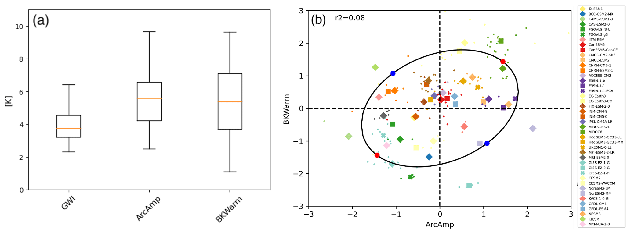
Figure 1(a) Boxplot showing the global warming index (GWI), and the two predictor indices used for the storylines (ArcAmp and BKWarm). GWI is defined as the global and annual mean response of the 2 m temperature, ArcAmp is the response of the 850 hPa temperature averaged over all regions poleward of 55° N, and BKWarm is the response of the sea surface temperature averaged over the Barents–Kara seas (units: K). Both ArcAmp and BKWarm are defined for the extended summer season (May to October). The response is defined as the climatological mean difference in the last 30 years of the current century (2070–2099) with that of the historical period (1985–2014). The lowest and highest values are shown at the extremities of each box; box delimiters define the 25th and 75th percentiles, while the median value (50th percentile) is shown by an orange line. (b) ArcAmp and BKWarm normalised by the GWI and with the MMM value removed for each model. Note that each predictor index is rescaled by its standard deviation and thus non-dimensionalised (e.g. a value of 1 means a difference of 1 standard deviation from the MMM value). The solid ellipse delimits the 80 % confidence region of the model response in ArcAmp and BKWarm (Eq. 3). Dots on the ellipse show the four storylines defined in Eqs. (3a)–(3d).
2.1 Model data
Our analysis uses a set of 43 climate models from CMIP6 (Eyring et al., 2016) which we downloaded from the Earth System Grid Federation (ESGF; Cinquini et al., 2014; models with members are listed in Table 1). The model and number of ensemble members (given in parentheses) include: TaiESM1 (1), BCC-CMS2-MR (1), CAMS-CSM1-0 (2), CAS-ESM2-0 (2), FGOALS-f3-L, FGOALS-g3 (4), IITM-ESM (1), CanESM5 (15), CanESM5-CanOE (3), CMCC-CM2-SR5 (1), CMCC-ESM2 (1), CNRM-CM6-1 (6), CNRM-ESM2-1 (5), ACCESS-CM2 (5), E3SM-1-0 (5), E3SM-1-1 (1), E3SM-1-1-ECA (1), EC-Earth3 (15), EC-Earth3-CC (1), FIO-ESM-2-0 (3), INM-CM4-8 (1), INM-CM5-0 (1), IPSL-CM6-LR (7), MIROC-ES2L (10), MIROC6 (15), HadGEM3-GC31-LL (4), HadGEM3-GC31-MM (4), UKESM1-0-LL (5), MPI-ESM1-2-LR (15), MRI-ESM2-0 (6), GISS-E2-1-G (14), GISS-E2-2-G (5), GISS-E2-1-H (10), CESM2 (3), CESM2-WACCM (3), NorESM2-LM (1), NorESM2-MM (1), KACE-1-0-G (3), GFDL-CM4 (1), GFDL-ESM4 (1), NESM3 (2), CIESM (1), and MCM-UA-1-0 (1). For each model, all ensemble members of the historical experiment that were extended into the SSP5-8.5 scenario are used and capped to a maximum of 15 members per model to limit computational resources needed to produce ensemble means for the few models that have many members. As most models only have a few members, setting a maximum of 15 members seems a reasonable trade-off for reducing internal variability while including as many models as possible. We find little difference in using only a single member or an ensemble mean of members as the climate projections are dominated by the effect of the climate forcing with only a small contribution from natural variability (see Fig. 1b). For each model, we produce a mean climatology of the ensemble members for both the historical and SSP5-8.5 experiment, in their respective period of evaluation (i.e. 1985–2014 and 2070–2099), to reduce the weight of internal variability in the climate projections. Therefore, every model is represented by one climate projection regardless of their number of members or whether it is a single member or an ensemble-mean of members.
2.2 Multivariate linear regression analysis
The climate storyline approach is based on a multivariate linear regression (MLR) analysis that expresses the response to global warming of any variable, Z (“target variable”), as a linear superposition of its response to changes in N climate indices, Pi (“predictor index”). Following the methodology outlined in Zappa and Shepherd (2017), this can be expressed as follows:
Here, ΔZ defines changes in target variable Z, ΔPi defines changes in predictor index Pi, and βi is the response of variable Z to changes in Pi. Note that the target variable Z varies both in space [x] and across models [m], but predictor indices Pi only vary across models; predictor indices are typically the regional averages of variables that are tied to well-known physical features of the climate. defines a multi-model ensemble mean (MMM), and defines a deviation from the MMM. Δ defines the difference in climatology between the 2070–2099 (SSP5-8.5 emission scenario) and 1985–2014 (historical experiment) period normalised by a global warming index (Tssp585−Thist), that is,
Here, T is the annual global mean 2 m air temperature, and X defines any target variable or predictor index. Normalisation ensures that changes in the target variables and predictor indices are not directly associated with changes in the global warming index (GWI; with ). Instead, the normalised response describes the variability in target variables or predictor indices linked to the underlying changes in the dynamics of the atmosphere, ocean, or ice triggered by global warming, rather than the variability directly affected by the model's climate sensitivity.
Storylines are constructed using the coefficients βi emerging from the MLR analysis (Eq. 1a) which are compounded with a standardised climate response for each predictor. In a two-predictor MLR analysis, this amounts to the creation of four storylines that are representative of the diversity in the climate change response across CMIP6 models:
Here, s defines the standardised climate response, whose value is set to 1.26. This value is derived from a chi-squared distribution for 2 degrees of freedom and evaluated on the edge of the 80 % confidence boundary region; this distribution is applied to the standardised inter-model spread in our two predictors from the large ensemble of CMIP6 simulations described in Sect. 2.1. In simpler terms, s defines a standardised deviation from the MMM of equal magnitude in our two-predictor indices, which we deem plausible and yet not so extreme to be unlikely, based on the projection spread across CMIP6 simulations. To account for a weak positive correlation between both predictor indices, the storylines in Eq. (3) also contain the factors Γ and γ which depend on the correlation coefficient r (see M20 for more details).
The MLR framework of Eqs. (1a) and (3) seeks to predict the inter-model variability in the projections and not the multi-model ensemble mean climate response; this is borne out of our storylines' aim to explore a range of possible climate realisations representative of the diversity in model projections. While the MLR framework is compatible with using any number of predictor indices, the exponential increase in storylines with the number of predictors (2N storylines can be produced for a set of N predictors) prompts us to use as few predictors as necessary to keep the number of storylines tractable. We limit ourselves to two predictors and four storylines as our analysis demonstrates that this configuration can explain a large fraction of the inter-model spread in the warming response of the Arctic (Table 1).
2.3 Choice of target variables
Due to their relevance to a broad array of climate risks, we select 2 m temperature, precipitation rate, 850 hPa zonal wind, and sea ice fraction as target variables for understanding the impact of Arctic climate change (Lee et al., 2022). Note that the 850 hPa zonal wind is considered to be a good proxy for the near-surface wind while being less sensitive to the physical parameterisation of surface processes (e.g. ZS17). This choice of variables is highly relevant to many key climate-driven risks in the Arctic, including wildfires, permafrost thawing, sea ice loss, and marine heatwaves (Anisimov and Nelson, 1997; Pabi et al., 2008; Arrigo and Van Dijken, 2015; Melia et al., 2016). For instance, Arctic wildfires are sensitive to warm, dry, and windy conditions, which implies a dependence on near-surface air temperature, near-surface wind, and precipitation accrued during the warm season (Dowdy et al., 2010). We define 2 m temperature as our reference target variable because of its preponderance in driving those climate risks. This means that our storylines are optimised to represent the variability in the 2 m temperature.
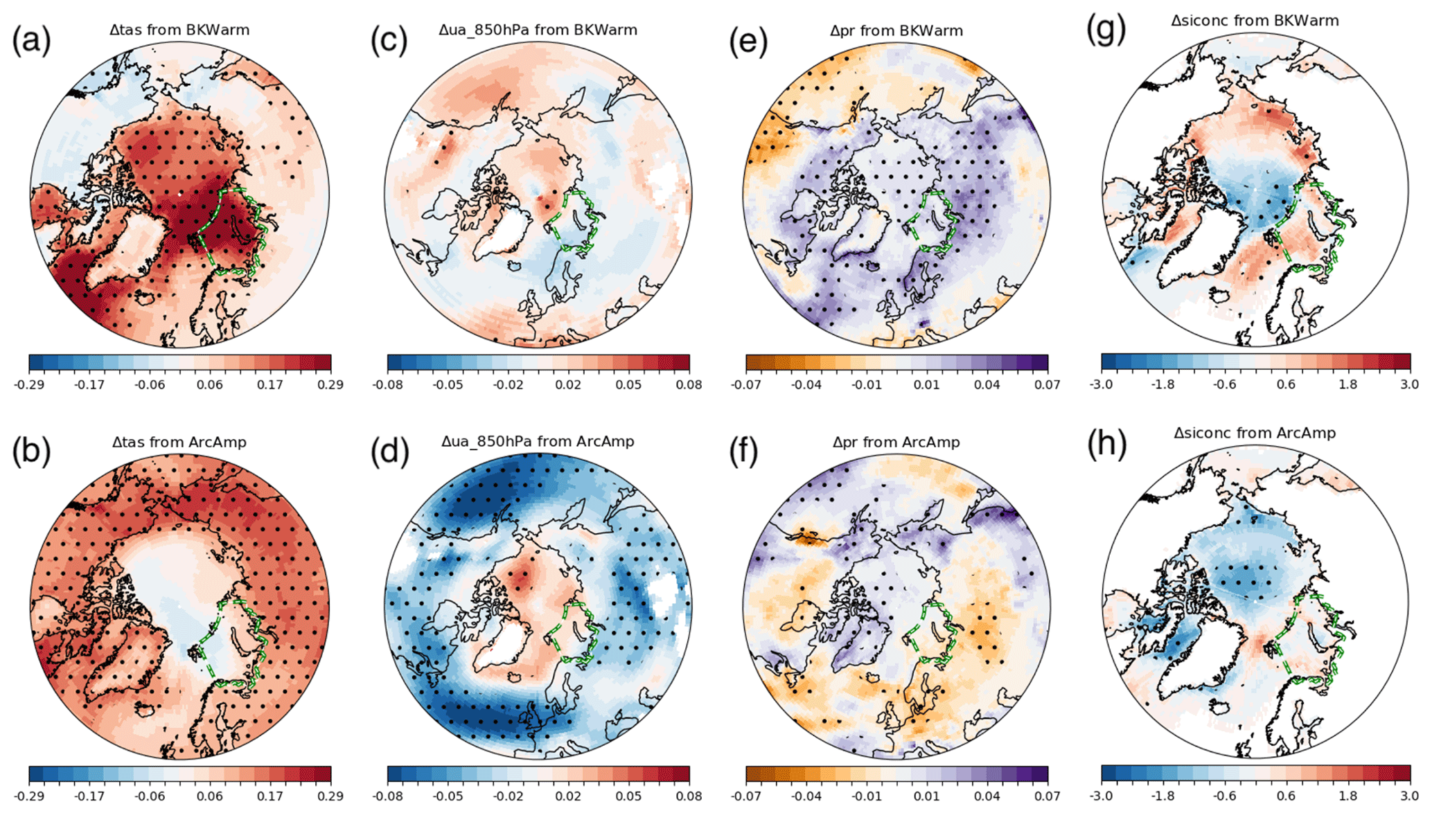
Figure 2Normalised response of (from left to right) 2 m temperature [K K−1], 850 hPa zonal wind [], precipitation rate [], and sea ice fraction [% K−1] to 1 standard deviation in each of the predictor index for BKWarm (a, c, e, g) and ArcAmp (b, d, f, h). The normalised response is the product of the regression coefficient βi in Eq. (1a) with and 1 standard deviation anomaly in the associated predictor index. Stippling indicates statistical significance at the 95 % confidence level using Student's t test (i.e. p value less than 0.05). The dashed green line delineates the outline of the Barents–Kara seas.
2.4 Choice of predictor indices
Using the MLR approach, the target variables' response to global warming may be regressed upon the two climate indices that we consider optimal for explaining differences in climate change projections between the CMIP6 model simulations. In this study, we select Arctic atmospheric amplification and Barents–Kara sea warming as our predictors, which we refer to, respectively, as “ArcAmp” and “BKWarm”. ArcAmp is defined as the 850 hPa temperature change averaged over all areas poleward of 55° N and BKWarm as the sea surface temperature change averaged over the Barents–Kara seas (its outline is shown in Fig. 2). Both ArcAmp and BKWarm are defined over the extended summer season (May to October). We choose these two predictors owing to their ability to explain a large fraction of the inter-model variability in climate change projections in the Arctic, specifically the warming of the boundary layer over marine and terrestrial regions. Indeed, comparing 850 hPa temperature against surface temperature in the Arctic regions shows a strong covariability over land but weak covariability over marine areas (see Fig. 2a and b), consistent with the thermal decoupling of the marine boundary layer from the free troposphere in summer (e.g. Tjernström and Graversen, 2009). Over ocean regions, the warming of the marine boundary layer is found to warm coherently across the central Arctic, Barents–Kara, and North Atlantic regions (Fig. 2a), in agreement with a coherent increase in sea surface temperature across those regions. Due to its role as a climate gateway between the North Atlantic and the Arctic oceans (e.g. Smedsrud et al., 2013), we select the Barents–Kara seas as our reference region for defining our ocean warming predictor in the Arctic. Conversely, we select the 850 hPa Arctic mean temperature warming as our second predictor due to its high degree of covariability with the warming of the terrestrial boundary layer and low degree of covariability with the marine boundary layer warming (see Table B1). The processes tying temperature anomalies in the free troposphere to those of the surface over land likely involve multiple atmospheric feedback, such as radiative or boundary layer mixing changes, which is beyond the scope of this study. Likewise, while our study leverages the connections among the North Atlantic Ocean, Barents–Kara seas, and central Arctic Ocean warming to produce a predictor for marine boundary layer warming (see Table B2), it does not seek to identify a mechanism connecting these three regions as it would require an in-depth analysis of changes in ocean current, upper-ocean mixing, and surface fluxes.
Figure 1a shows the inter-model spread in ArcAmp, BKWarm, and GWI, which is of comparable magnitude to their MMM value for all three indices; yet we note that the spread is larger for ArcAmp and BKWarm than GWI. This large spread reflects known uncertainties in the warming of the Barents–Kara seas and the lower Arctic troposphere in climate models which are associated with poorly constrained physical processes and teleconnections influencing the Arctic climate (e.g. Previdi et al., 2021). Figure 1b shows ArcAmp and BKWarm for all CMIP6 models, which shows a weak correlation in their values (r2=0.08); this is made evident by the elliptically shaped confidence boundary region in Fig. 1b which accounts for the larger spread in variance along the direction of correlation (the ellipticity is determined by the Γ and γ factors in Eq. 3). This nearly satisfies an important condition of orthogonality necessary for the effective combined use of ArcAmp and BKWarm as predictors in the MLR framework (Eq. 1a). The near-independence in the changes in ArcAmp and BKWarm suggests that the sensitivity of the Barents–Kara seas and that of the lower troposphere (850 hPa) to global warming is controlled by different physical processes – even if changes in both predictor indices are ultimately driven by global warming.
Applying the two-predictor MLR framework described in Eq. (1a), we find that the inter-model variance in the 2 m temperature explained by ArcAmp and BKWarm describes close to half of its overall inter-model variance over the Arctic (41 %; see Table 1). This is about two-thirds of the theoretical maximum that can be explained using a two-predictor MLR (64 %) which we evaluated as the variance explained by the first two components of a principal component analysis (PCA) applied on the normalised change in 2 m temperature (Table 1; top row). Applying the same framework to explain changes in the 850 hPa zonal wind, precipitation rate, and sea ice fraction, we find that the amount of variance explained by our two-predictor MLR is substantially lower (∼ 15 %) for these variables, even if it is not insignificant. Nevertheless, evaluating the fraction of variance explained by the MLR framework on regional-scale changes (either over the Arctic or broader Northern Hemisphere high latitudes) generally indicates that our storylines have a larger explanatory power when applied to spatially coherent changes in our target variables, strengthening the relevance of our Arctic storylines to variables other than 2 m temperature (Table 1; bottom row). This highlights the fact that our storylines are tailored to quantitatively describe changes in the near-surface warming and can only provide a qualitative picture of the changes in those three variables.
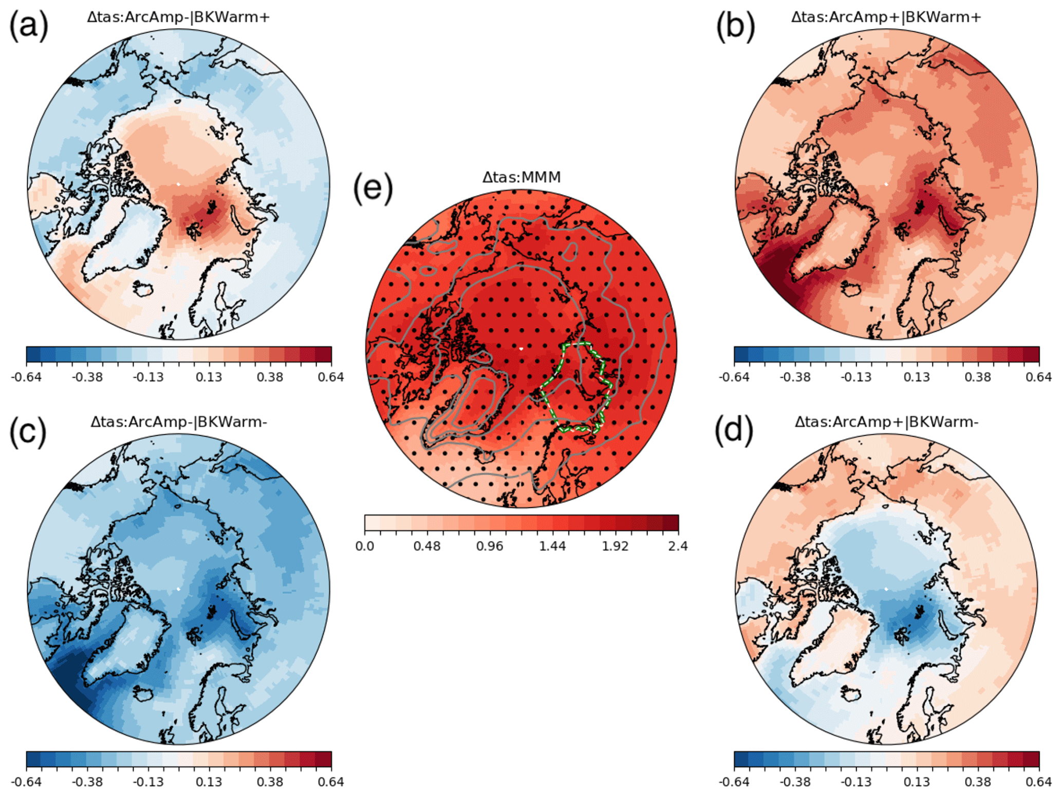
Figure 3(a–d) Storylines of climate change for 2 m temperature as defined in Eqs. (3a)–(3d) and (e) its MMM projection (units: K K−1). Stippling in panel (e) indicates areas where at least 80 % of the models agree on the sign of change, and solid grey contours indicate the MMM present-day climatology. The dashed green line delineates the outline of the Barents–Kara seas.
Figure 2 shows the normalised response of each target variable in the extended summer season to each predictor index that is the response per degree of global warming for 1 standard deviation in the inter-model spread of the predictor index. A warm anomaly in the Barents–Kara seas (BKWarm) is associated with the following: a warm anomaly in the 2 m temperature over the central (marine) Arctic (Fig. 2a); a dipolar anomaly in the 850 hPa zonal wind changes, with weaker winds over the Atlantic sector of the Arctic but stronger winds over the Pacific sector (Fig. 2c); positive anomalies in precipitation rates across all Arctic regions, especially so over land areas (Fig. 2e); and accelerated rates of sea ice loss in the central Arctic but reduced rates of sea ice loss the Pacific sector of the Arctic and Barents–Kara seas (Fig. 2g). We note that the sea ice extent in the Barents Sea region appears to be increasing in response to Barents–Kara sea warming (Fig. 2g); this is a counter-intuitive finding that is likely an artefact of the low number of models having sea ice cover in summer in this region, as suggested by the lack of statistical significance in the response.
These normalised response patterns strongly contrast with that associated with warm anomalies of the lower troposphere in the Arctic (ArcAmp). For warm anomalies in ArcAmp, we find 2 m temperature increases over most terrestrial areas (Fig. 2b), the 850 hPa zonal wind weakens over most areas around the Arctic but strengthens in the central Arctic (Fig. 2d), precipitation rates are reduced over most high-latitude land areas except over Greenland and the Bering Strait regions (Fig. 2f), and sea ice loss is reduced in the central Arctic and the Pacific sector of the Arctic basin (Fig. 2h). Both 2 m temperature and precipitation rates response to ArcAmp are opposite to that associated with warm anomalies over the Barents–Kara seas. This difference in the normalised response to BKWarm and ArcAmp reflects important differences in how our two predictor indices can modulate climate change and explain the diversity of model projections found under the SSP5-8.5 scenario forcings.
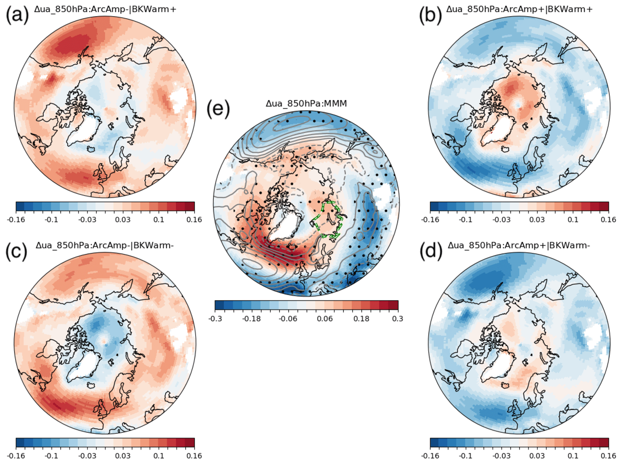
Figure 4Storylines of climate change for the 850 hPa zonal wind (a–d) and its MMM projection (e) (units: ). The same convention as Fig. 3 applies.
Using these normalised responses to each predictor index, we produce four storylines for each of the four target variables according to Eq. (3). Specifically, we describe the following four storylines, referenced from A to D and defined in Eq. (3): A is for ArcAmp−/BKWarm+, B is for ArcAmp+/BKWarm+, C is for ArcAmp−/BKWarm−, and D is for ArcAmp+/BKWarm−. Figure 3 shows the storylines of the 2 m temperature change. First, we note that the storylines' patterns are qualitatively similar to those obtained from the two first modes of the PCA for the 2 m temperature change (compare Fig. 3a–d with Fig. A1a–d); this confirms that our ArcAmp and BKWarm predictors capture well the dominant modes of variability that drive the inter-model spread in surface warming projections. Consistent with the normalised response patterns (Fig. 2a and b), the main difference in 2 m temperature between the four storylines is the rate of warming between marine and terrestrial areas of the Arctic (Fig. 3). In the MMM, the 2 m temperature is found to increase by about 1.5 to 2 K K−1 over most oceanic and terrestrial areas of the Arctic (Fig. 3e), showing a relative uniformity in magnitude across the Arctic. For positive anomalies in both BKWarm and ArcAmp, i.e. storyline B, the rate of warming is increased over most Arctic areas (Fig. 3b); the opposite situation is found in storyline C, i.e. negative BKWarm and ArcAmp anomalies, with a reduced rate of warming over most Arctic areas (Fig. 3c). For positive (negative) anomalies in BKWarm but negative (positive) anomalies in ArcAmp, i.e. storyline A (D), the rate of warming is increased (reduced) over marine areas but reduced (increased) over terrestrial areas when compared to the MMM (compare Fig. 3a with Fig. 3d). Changes are stronger over marine areas, especially in the northern part of the Barents–Kara seas and the western North Atlantic basin, where values can depart by up to 30 % compared to the MMM. Out of all four storylines, storylines A and D show the largest deviation in warming rates between terrestrial and marine areas (Fig. 3a and d). Beyond an amplification or dampening of the MMM climate response, our analysis suggests a decoupling of the near-surface temperature warming between terrestrial and marine areas, with the former being associated with the lower-tropospheric warming and the latter connected to changes in the Barents–Kara and North Atlantic basin.
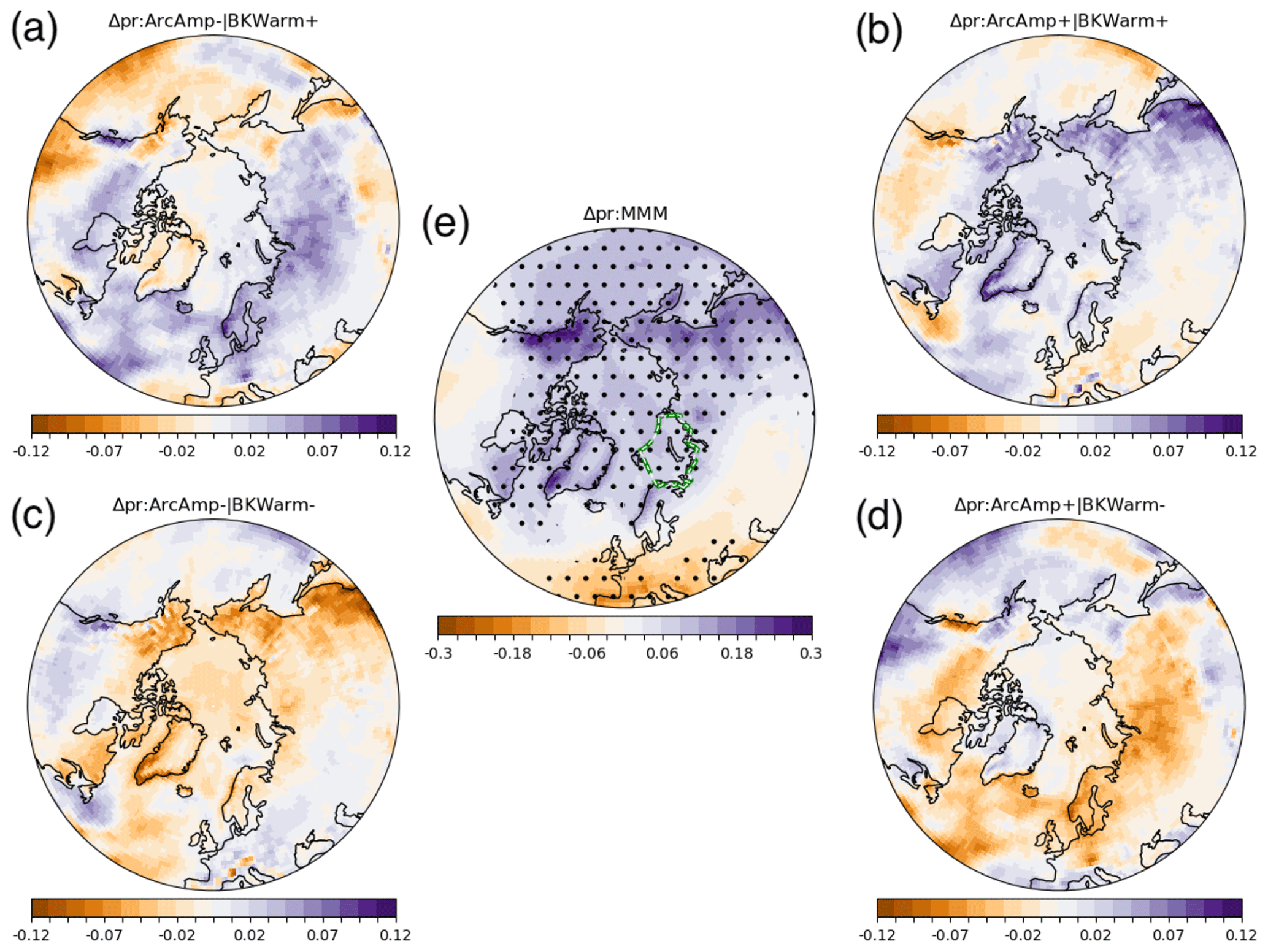
Figure 5Storylines of climate change for precipitation (a–d) and its MMM projection (e). The same convention as Fig. 3 applies.
In comparison with the 2 m temperature, changes in the 850 hPa zonal wind show more complexity in the spatial pattern of changes between the four storylines. In the MMM, the change in the 850 hPa zonal wind (U850) shows westerly tendencies across a wide area in the circumpolar regions, spanning eastward from the Bering Sea to the Barents–Kara seas, with a maximum over the North Atlantic between southern Greenland and Scandinavia. The westerly tendencies extend to the Pacific sector of the Arctic Ocean, forming an arch stretching from the Beaufort Sea to the Laptev Sea. On the other hand, easterly tendencies are found in the midlatitude regions of central Siberia. Overall, those changes suggest that in the MMM, westerly winds shift poleward and strengthen around the subpolar front and in the central Arctic, in qualitative agreement with previously noted changes in the Northern Hemisphere mid- and high-latitude regions (Harvey et al., 2020). Going beyond the multi-model mean changes, storylines indicate a strong modulation of those changes, with the storyline changes being up to 50 % of the MMM. As for the 2 m temperature, storylines of U850 show the modulation of the MMM response departing from a simple amplification response. Storylines B and C show a bipolar pattern (Fig. 4b and c) with an easterly (westerly) tendency in the circumpolar regions but westerly (easterly) tendencies over the Arctic ocean in B (C). Likewise, storylines A and D show an apparent bipolar pattern in the climate response, with changes in the subpolar regions being of opposite signs to that found in the Norwegian and Barents Sea (Fig. 4a and d). Relative to the multi-model mean changes, the poleward shift in the North Atlantic storm tracks is influenced primarily by Arctic atmospheric warming, hence linking the large uncertainty in its prediction across climate models to the inter-model spread in ArcAmp. For instance, a strengthening of the 850 hPa zonal wind in the subpolar region occurs when ArcAmp weakens, consistent with polar atmospheric warming weakening the storm tracks (e.g. Smith et al., 2019). Even if our storylines account for only a fraction of the model spread in the 850 hPa zonal wind projections, the different outcomes outlined by our storylines suggest markedly different impacts of global warming on the low-level winds, with implications for changes in synoptic storms' tracks and intensity changes.
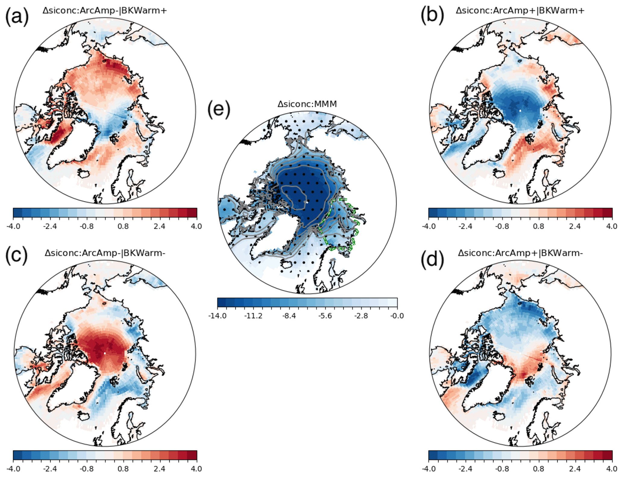
Figure 6Storyline of climate change for sea ice fraction (a–d) and its MMM projection (e).
Figure 5 confirms the expected increase in precipitation rate changes in the high-latitude regions in the MMM. This increase is most pronounced over mountain ranges found on the western sides of continents which are on the paths of the Atlantic and Pacific storm tracks, e.g. the North American coastal ranges, western Greenland, and Scandinavian coastal ranges (Fig. 5e). This increase in precipitation rate contrasts with the drying tendency found over most of the midlatitude and subtropical regions of Eurasia and North America. Storylines show that projections can differ substantially from this pattern by up to 50 % of the MMM values. In particular, the precipitation rate increases over most of the Arctic for positive anomalies in BKWarm (Fig. 5a and b) but decreases for negative anomalies in BKWarm (Fig. 5c and d). Changes over terrestrial areas are generally of greater amplitude than over marine areas across all storylines and most particularly over regions of strong rainfall in the present-day climate. Overall, storylines of precipitation rates are modulated primarily by change in BKWarm, with only specific regions – notably Greenland and Siberia – showing a response to ArcAmp.
Figure 6 confirms the expected decline in sea ice across the Arctic in the MMM, with sea ice fraction displaying loss by at least 15 % (see Fig. 6e). However, our storylines reveal a more complex picture than suggested by the MMM. On the one hand, central Arctic amplification or dampening of these changes occur when BKWarm and ArcAmp changes are additive (Fig. 6b and c). On the other hand, large regional contrasts can appear when BKWarm and ArcAmp changes are of the opposite sign (Fig. 6a and d); this is especially obvious when comparing the Atlantic and Pacific sectors of the Arctic. Those changes appear to be associated largely with the Arctic atmospheric warming, with the Barents–Kara sea warming playing a more local role with its effect being felt primarily in the Atlantic sector of the Arctic Ocean.
We produced four summertime climate change storylines for the Arctic region for the four target variables that we consider to characterise seasonal change in the surface climate: 2 m temperature, precipitation rate, zonal wind at 850 hPa level, and sea ice fraction over the Arctic region. We devised those storylines using an established methodology previously applied to develop storylines across various midlatitude regions of both hemispheres (ZS17; ML20). We combined this framework with the realisation that Arctic climate change in summer is tightly associated with two climate indices, the Barents–Kara sea warming (BKWarm) and Arctic atmospheric amplification (ArcAmp), which we used as predictors. Our choice of methodology and predictors was guided by two criteria: (i) our storylines should be representative of the diversity in model projections, and (ii) our predictors should be connected to physical processes. Criterion (i) ensures that the storylines capture a meaningful set of possible climate change realisations, while criterion (ii) allows for a scientific understanding of what drives this diversity in model projections. Criterion (i) is critical to the viewpoint of the end-users who need a plausible range of climate change scenarios, for instance, to develop mitigation strategies, while criterion (ii) is of greater interest to scientists who desire insights regarding the drivers of climate change in the Arctic. When based on those two criteria, storylines can be used to study possible impacts of climate changes, as well as categorise climate models by storylines; as such, storylines are an efficient way of identifying a few climate models most representative of the diversity of CMIP6 projections.
Our storylines are particularly successful at capturing the spread in model projections for the 2 m temperature; our primary finding is the differential warming rates between terrestrial and marine areas, which we find to be a major source of divergence in model projections. We also applied our storyline analysis to other variables with a varying degree of success; the relevance of storylines to each target variable must be assessed on a case-by-case basis as different target variables may be controlled by distinct processes. Likewise, our predictors are less successful at capturing changes in seasons other than the extended boreal summer. The specificity of storylines to variables, seasons and regions is an important limitation of this methodology, as it relies on careful tuning to comprehensively represent changes.
Using this methodology, we produced the four Arctic climate change storylines: ArcAmp−/BKWarm+ (A), ArcAmp+/BKWarm+ (B), ArcAmp−/BKWarm− (C), and ArcAmp+/BKWarm− (D). Our storylines show noticeably different paths for Arctic climate change, which deviate substantially from the multi-model ensemble mean. Compared to the MMM, the cooler surface temperature in storylines A and C suggests fewer fire risks and less extensive permafrost thawing if undergoing the same amount of global warming. Storylines B and D present the opposite outcome with more intense land warming that may lead to greater fire risks and more permafrost thawing. Concomitant changes in precipitation rates and surface wind are expected to modulate those trends; for instance, a wetter summer could imply a reduced fire risk in storyline B compared to D, even if both storylines show similar rates of warming over land. The combined impacts of physical changes at the surface on climate risks such as fires and permafrost thaw can only be evaluated with a quantitative analysis that is beyond the scope of our study. Furthermore, our analysis also shows that enhanced risks over land may or may not translate into enhanced impacts over marine areas. For instance, storyline A – which showed a lessening of climate risks over land – is tied to an enhanced warming of the Arctic Ocean and an amplified loss of sea ice cover, suggesting a more navigable Arctic Ocean and greater disruptions in marine primary production compared to the MMM. Beyond changes that may be consistent across the entire Arctic, the storylines also suggest futures in which regional contrasts are enhanced. For instance, storylines A and D show that sea ice cover shrinking may have pronounced differences between the Pacific and Atlantic sectors of the Arctic Ocean; such changes would likely entail regional differences in the volume of Arctic shipping or marine primary production. Overall, we demonstrate that storylines can be used to better understand the range of possible climate outcomes for the Arctic that emerge from coupled climate models, a critical step toward planning for climate adaptation strategies.
We also tested an empirical method for producing storylines in which predictor indices emerge from a principal component analysis (PCA). This is achieved by finding the first two components of a PCA applied to each target variable (von Storch and Zwiers, 2002) and using those as predictors. Specifically, we can express changes in a target variable ΔZ as
Here, EOFi is the eigenmode and PCi the eigenvalues of the ith mode, and the summation is done over N principal components. As in the MLR storylines (Eq. 1a), the PCA storylines describe the inter-model variability in model projections with respect to the MMM changes. Comparing the two frameworks, we find that eigenmode EOFi(x) in Eq. (A1) is analogous to coefficient βi(x) in Eq. (1a), and PCi(m) in Eq. (A1) is analogous to climate predictor in Eq. (1a). Following the same methodology to the physical storylines, we produce four “empirical” storylines as follows:
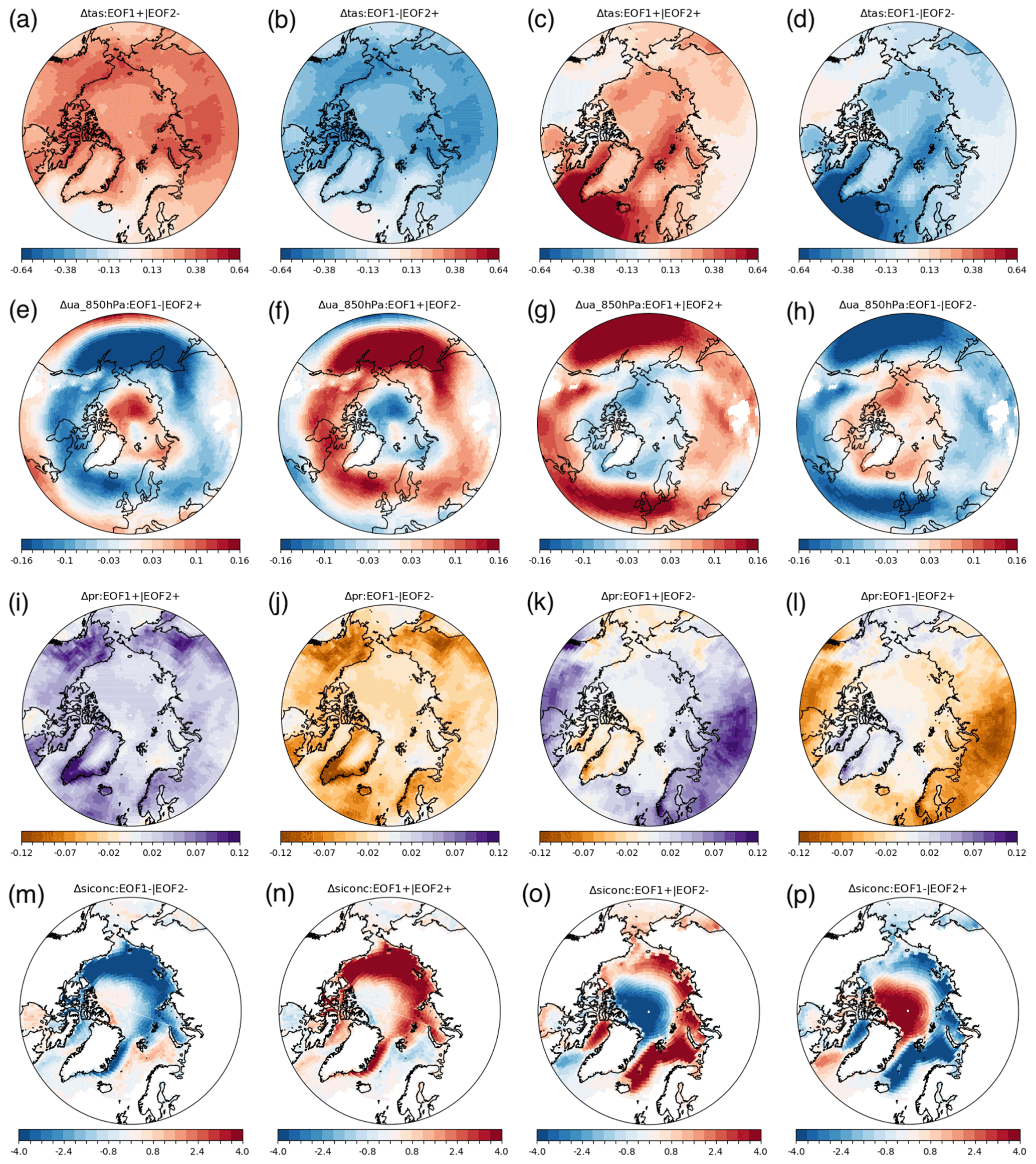
As in Eq. (3), s defines the standardised climate response in Eq. (A2), which is derived from a chi-squared distribution for 2 degrees of freedom and evaluated on the edge of the 80 % confidence boundary region (s=1.26). Compared to the two-predictor MLR storylines (Eq. 3), the two-component PCA storylines (Eq. A2) will better discriminate the spread in model projections, since the variance explained by the first two components of a PCA maximises the variance that can be explained in the inter-model spread from any two predictors. While PCA predictors present the advantage of being strictly orthogonal to each other by construction, they are not directly relatable to specific climate indices or physical processes, which is a substantial drawback for interpreting changes. For these reasons, empirical storylines may be useful for providing a representative range of climate outcome to end-users (perhaps even more so than the MLR storylines if judging solely from the amount of variance explained); however, they are likely to be less relevant for understanding the underlying processes driving the diversity in climate outcomes.
Empirical storylines show qualitative similarities with the storylines presented in our study (see Fig. A1) to those found in our physical storylines for most target variables (Fig. 3–6), even if physical storylines consistently underperform empirical ones with regard to the amount of explained variance in model projections. This is particularly true for the 2 m temperature, which shows very similar patterns between empirical storylines and our storylines (compare Fig. A1 and Fig. 3).
We selected the predictors for our Arctic storylines based on their ability to represent changes in key surface climate variables in a linear regression framework. This entails that our two predictors should maximise the variance explained by the MLR model while being as weakly correlated as possible (orthogonality of predictors is not strictly necessary but remains convenient for interpreting changes). We already motivated in Sect. 2.4 that lower-tropospheric temperature change (represented by ArcAmp) and sea surface warming at high latitudes (represented by BKWarm) are the most relevant factors for defining our two predictors; however, we did not explain the specific choices of pressure level or area for evaluating ArcAmp or BKWarm.
Table B1 shows the variance explained by the MLR model when using as predictors BKWarm (as defined in Sect. 2.4) and ArcAmp (as defined in Sect. 2.4 but using the pressure level value shown in top row). Table B1 also shows the correlation coefficient between BKWarm and ArcAmp at various levels.
Compared with other vertical levels, Table B1 shows that temperature at the 850 hPa level is only weakly correlated with the Barents–Kara sea warming (0.08; see bottom row in Table B1) and also nearly maximises the MLR explained variance (0.41; see top row in Table B1). Specifically, the MLR explained variance is found to decrease from a maximum value of 0.43 at 925 hPa to lower values higher in the troposphere, while the predictor correlation decreases swiftly above the lowest-tropospheric level (1000 hPa), which makes the 825 hPa level a reasonable choice for defining ArcAmp. We also note that the 825 hPa pressure level was selected to define Arctic amplification in past studies (e.g. Manzini et al., 2014; ZS17).
Table B1The top row shows the explained variance (R2) for the 2 m air temperature over the Arctic by the multivariate linear regression model, using BKWarm and ArcAmp as predictors for various evaluation levels of ArcAmp. The bottom row shows the correlation (r2) of BKWarm with ArcAmp for various levels of evaluation of ArcAmp (columns) ranging from the lowest model level (1000 hPa; leftmost column) to the mid-troposphere (500 hPa; rightmost column).
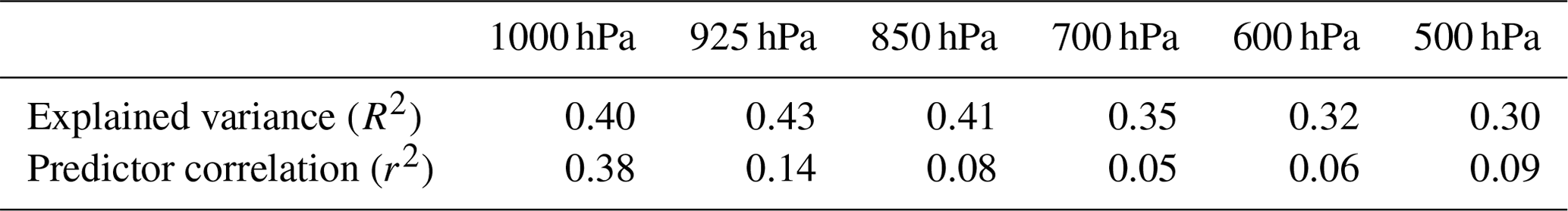
Table B2The same as Table 1 but using various oceanic regions for our BKWarm predictor in the Barents–Kara seas (left column; [65° N, 80° N, 26° E, 95° E]; ocean only), central Arctic Ocean (middle column; [70° N, 90° N, 180° W, 180° E]; ocean only), and North Atlantic Ocean (right column; [45° N, 60° N, 70° W, 0°]; ocean only).
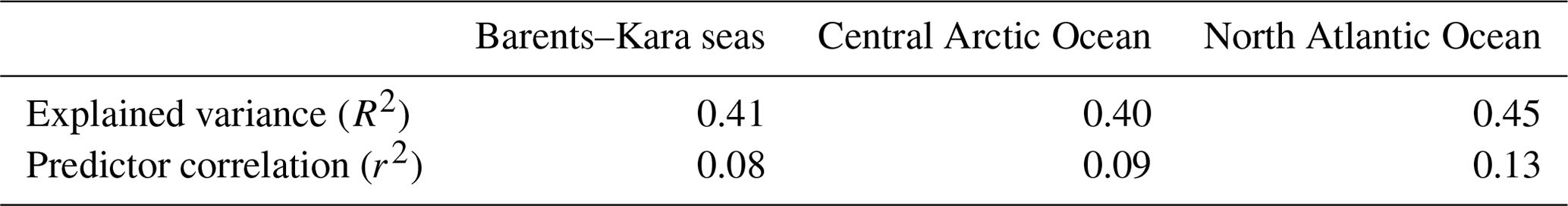
Similar to Table B1, we compare the variance explained by the MLR model and correlation coefficient when using as predictors ArcAmp (as defined in Sect. 2.4) and sea surface warming averaged over various areas of the Northern Hemisphere (including the Barents–Kara seas), as shown in Table B2. In addition to the Barents–Kara seas, we tested the central Arctic and North Atlantic ocean warming because of their covariability with Barents–Kara sea warming (Fig. 2a) and because of their being areas where inter-model variability in sea surface warming is the strongest at high latitudes (Fig. A1a–d).
Table B2 shows similar values for the MLR explained variance and predictor correlation when selecting either central Arctic, North Atlantic, or Barents–Kara sea warming. Based on this criterion alone, any of those three region could have been chosen as predictors for our Arctic storylines. Ultimately, we selected the Barents–Kara seas as the reference area for defining our predictor because of its mediating role between the North Atlantic and the Arctic ocean warming (e.g. Smedsrud et al., 2013), as explained in Sect. 2.4.
Nearly all studies using the storyline approach show the total storyline patterns (e.g. ZS17) which correspond to the response of the target variables to each predictor added upon the multi-model mean (MMM) change. Showing the full response is most relevant to the end-users who study climate risks but can make it more challenging to distinguish what differentiates storylines because the storylines' patterns are strongly influenced by the common MMM change. For convenience, we provide the total storyline patterns, defined by adding the MMM change (normalised by the global and annual mean 2 m air temperature) to the storyline pattern defined in Eqs. (3a)–(3d) and shown in Figs. 3–6 for the 2 m air temperature (Fig. C1a–d), 850 hPa zonal wind (Fig. C1e–h), precipitation rate (Fig. C1i–l), and sea ice fraction (Fig. C1m–p). We comment on what differs between storylines in Sects. 3 and 4.
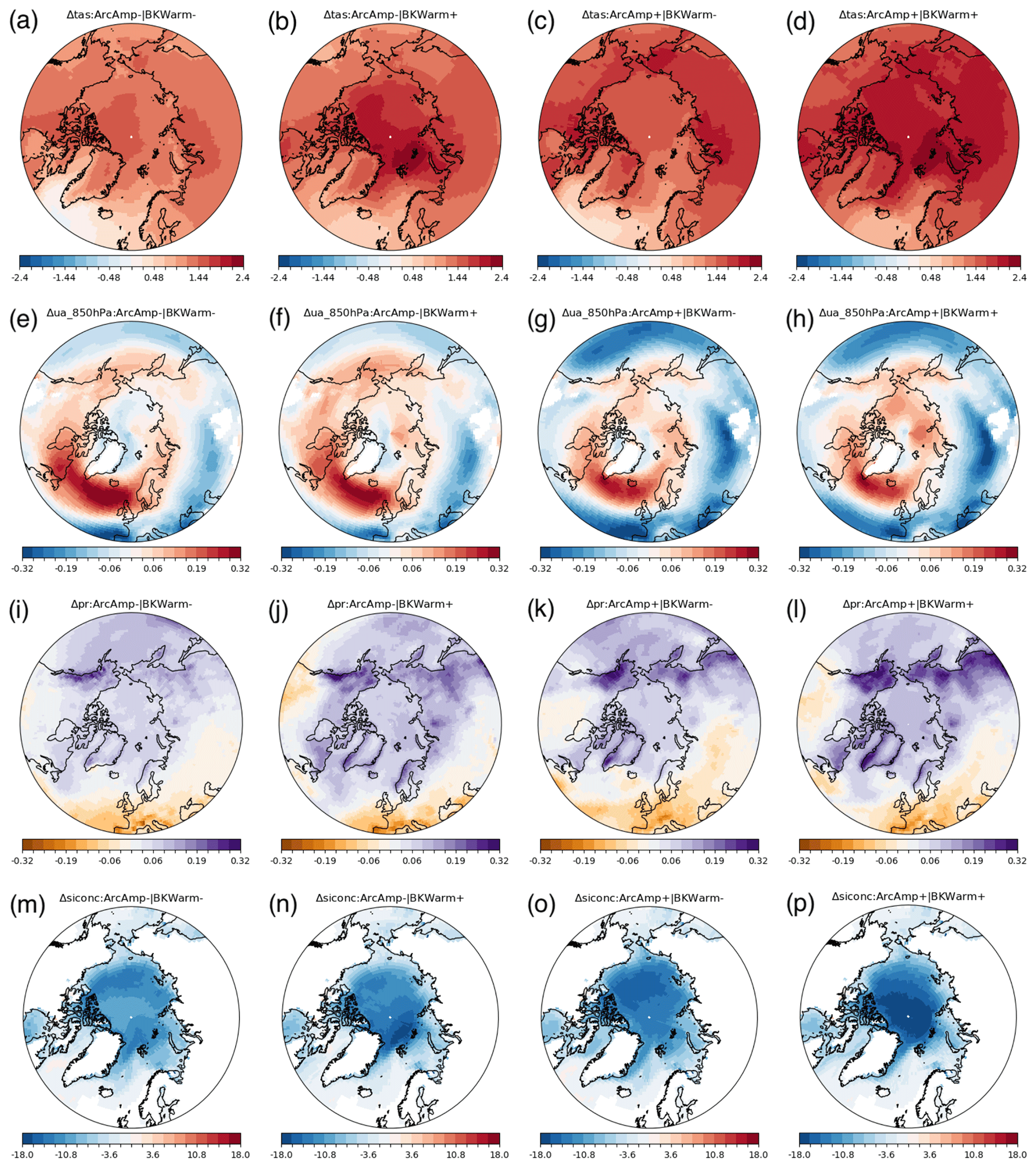
Figure C1Overall storylines of climate change for 2 m temperature, 850 hPa zonal wind, precipitation, and sea ice fraction. Overall storylines are defined by combining the multi-model ensemble mean change (Figs. 3e–6e) with our climate change storylines, as defined in Eq. (3), and with the patterns shown in panels a, b, c, and d of Figs. 3–6.
The code to produce the analysis shown in this study can be found on Zenodo (https://doi.org/10.5281/zenodo.12627367, Levine, 2024).
This study was based on World Climate Research Programme (WCRP)'s CMIP6 archived simulations, which can be found on the Earth System Grid Federation (ESGF, https://pcmdi.llnl.gov/CMIP6/, Lawrence Livermore National Laboratory, 2024). These data were stored locally on the National e-Infrastructure for Research Data (NIRD), a component of the Norwegian Research Infrastructure Services (NRIS).
XJL performed the formal analysis and was responsible for the data presentation, supervised efforts leading to this work, and was responsible for the preparation of the paper. XJL, RSW, GM, AO, LSG, and DH were instrumental in setting the main goals and structure of this study and setting the storyline methodology. NJ, HL, and LN provided important methodological inputs related to storylines' impact. RSW, GM, AO, LSG, DH, AK, RK, RRW, NJ, HL, LN, and PAM helped with the preparation of the draft, providing critical comments. PAM procured funding necessary to conduct this study and set the overarching goals of the PolarRES project that led to this study.
The contact author has declared that none of the authors has any competing interests.
Publisher's note: Copernicus Publications remains neutral with regard to jurisdictional claims made in the text, published maps, institutional affiliations, or any other geographical representation in this paper. While Copernicus Publications makes every effort to include appropriate place names, the final responsibility lies with the authors.
We acknowledge the support of PolarRES (grant no. 101003590), a project of the European Union's Horizon 2020 research and innovation programme. Storage and computing resources necessary to conduct the analysis were provided by Sigma2 – the national infrastructure for high-performance computing and data storage in Norway (project nos. NS8002K and NN8002K). The CMIP6 simulations used for this analysis were obtained from the Earth System Grid Federation (ESGF), an infrastructure supported by the World Climate Research Programme (WCRP).
This research has been supported by the EU H2020 Environment (grant no. 101003590).
This paper was edited by Ben Kravitz and reviewed by two anonymous referees.
Anisimov, O. A. and Nelson, F. E.: Permafrost zonation and climate change in the Northern Hemisphere: results from transient general circulation models, Climatic Change, 35, 241–258, 1997.
Arias, P. A., Bellouin, N., Coppola, E., Jones, R. G., Krinner, G., Marotzke, J., Naik, V., Palmer, M. D., Plattner, G.-K., Rogelj, J., Rojas, M., Sillmann, J., Storelvmo, T., Thorne, P. W., Trewin, B., Achuta Rao, K., Adhikary, B., Allan, R. P., Armour, K., Bala, G., Barimalala, R., Berger, S., Canadell, J. G., Cassou, C., Cherchi, A., Collins, W., Collins, W. D., Connors, S. L., Corti, S., Cruz, F., Dentener, F. J., Dereczynski, C., Di Luca, A., Diongue Niang, A., Doblas-Reyes, F. J., Dosio, A., Douville, H., Engelbrecht, F., Eyring, V., Fischer, E., Forster, P., Fox-Kemper, B., Fuglestvedt, J. S., Fyfe, J. C., Gillett, N. P., Goldfarb, L., Gorodetskaya, I., Gutierrez, J. M., Hamdi, R., Hawkins, E., Hewitt, H. T., Hope, P., Islam, A. S., Jones, C., Kaufman, D. S., Kopp, R. E., Kosaka, Y., Kossin, J., Krakovska, S., Lee, J.-Y., Li, J., Mauritsen, T., Maycock, T. K., Meinshausen, M., Min, S.-K., Monteiro, P. M. S., Ngo-Duc, T., Otto, F., Pinto, I., Pirani, A., Raghavan, K., Ranasinghe, R., Ruane, A. C., Ruiz, L., Sallée, J.-B., Samset, B. H., Sathyendranath, S., Seneviratne, S. I., Sörensson, A. A., Szopa, S., Takayabu, I., Tréguier, A.-M., van den Hurk, B., Vautard, R., von Schuckmann, K., Zaehle, S., Zhang, X., and Zickfeld, K.: Technical Summary, in: Climate Change: The Physical Science Basis. Contribution of Working Group I to the Sixth Assessment Report of the Intergovernmental Panel on Climate Change, edited by: Masson-Delmotte, V., Zhai, P., Pirani, A., Connors, S. L., Péan, C., Berger, S., Caud, N., Chen, Y., Goldfarb, L., Gomis, M. I., Huang, M., Leitzell, K., Lonnoy, E., Matthews, J. B. R., Maycock, T. K., Waterfield, T., Yelekçi, O., Yu, R., and Zhou, B., Cambridge University Press, Cambridge, United Kingdom and New York, NY, USA, 33−-144, https://doi.org/10.1017/9781009157896.002, 2021.
Arrigo, K. R. and van Dijken, G. L.: Continued increases in Arctic Ocean primary production, Prog. Oceanogr., 136, 60–70, 2015.
Callaghan, T. V., Johansson, M., Brown, R. D., Groisman, P. Y., Labba, N., Radionov, V., Barry, R. G., Bulygina, O. N., Essery, R. L., Frolov, D. M., and Golubev, V. N.: The changing face of Arctic snow cover: A synthesis of observed and projected changes, Ambio, 40, 17–31, 2011.
Chadburn, S. E., Burke, E. J., Cox, P. M., Friedlingstein, P., Hugelius, G., and Westermann, S.: An observation-based constraint on permafrost loss as a function of global warming, Nat. Clim. Change, 7, 340–344, 2017.
Cinquini, L., Crichton, D., Mattmann, C., Harney, J., Shipman, G., Wang, F., Ananthakrishnan, R., Miller, N., Denvil, S., Morgan, M., and Pobre, Z.: The Earth System Grid Federation: An open infrastructure for access to distributed geospatial data, Future Gener. Comp. Sy., 36, 400–417, 2014.
Cohen, J., Screen, J. A., Furtado, J. C., Barlow, M., Whittleston, D., Coumou, D., Francis, J., Dethloff, K., Entekhabi, D., Overland, J, and Jones, J.: Recent Arctic amplification and extreme mid-latitude weather, Nat. Geosci., 7, 627–637, 2014.
Dai, A., Luo, D., Song, M., and Liu, J.: Arctic amplification is caused by sea-ice loss under increasing CO2, Nat. Commun., 10, 121, https://doi.org/10.1038/s41467-018-07954-9, 2019.
Dowdy, A. J., Mills, G. A., Finkele, K., and de Groot, W.: Index sensitivity analysis applied to the Canadian forest fire weather index and the McArthur forest fire danger index, Meteorol. Appl., 17, 298–312, 2010.
England, M. R., Eisenman, I., Lutsko, N. J., and Wagner, T. J. W.: The recent emergence of Arctic Amplification, Geophys. Res. Lett., 48, e2021GL094086, https://doi.org/10.1029/2021GL094086, 2021.
Eyring, V., Bony, S., Meehl, G. A., Senior, C. A., Stevens, B., Stouffer, R. J., and Taylor, K. E.: Overview of the Coupled Model Intercomparison Project Phase 6 (CMIP6) experimental design and organization, Geosci. Model Dev., 9, 1937–1958, https://doi.org/10.5194/gmd-9-1937-2016, 2016.
Harvey, B. J., Cook, P., Shaffrey, L. C., and Schiemann, R.: The response of the Northern Hemisphere storm tracks and jet streams to climate change in the CMIP3, CMIP5, and CMIP6 climate models, J. Geophys. Res.-Atmos., 125, e2020JD032701, https://doi.org/10.1029/2020JD032701, 2020.
Hawkins, E. and Sutton, R.: The potential to narrow uncertainty in regional climate predictions, B. Am. Meteorol. Soc., 90, 1095–1108, 2009.
Hjort, J., Streletskiy, D., Doré, G., Wu, Q., Bjella, K., and Luoto, M.: Impacts of permafrost degradation on infrastructure, Nat. Rev. Earth Environ., 3, 24–38, 2022.
Ingvaldsen, R. B., Assmann, K. M., Primicerio, R., Fossheim, M., Polyakov, I. V., and Dolgov, A. V.: Physical manifestations and ecological implications of Arctic Atlantification, Nat. Rev. Earth Environ., 2, 874–889, 2021.
Jansen, E, Christensen, J. H., Dokken, T., Nisancioglu, K. H., Vinther, B. M., Capron, E., Guo, C., Jensen, M. F., Langen, P. L., Pedersen, R. A., and Yang, S.: Past perspectives on the present era of abrupt Arctic climate change, Nat. Clim. Change, 10, 714–721, 2020.
Jenkins, M. and Dai, A.: The impact of sea-ice loss on Arctic climate feedbacks and their role for Arctic amplification, Geophys. Res. Lett., 48, e2021GL094599, https://doi.org/10.1029/2021GL094599, 2021.
Jung, O., Sung, M. K., Sato, K., Lim, Y. K., Kim, S. J., Baek, E. H., Jeong, J. H., and Kim, B. M.: How does the SST variability over the western North Atlantic Ocean control Arctic warming over the Barents–Kara Seas?, Environ. Res. Lett., 12, 03402, https://doi.org/10.1088/1748-9326/aa5f3b, 2017.
Krikken, F., Lehner, F., Haustein, K., Drobyshev, I., and van Oldenborgh, G. J.: Attribution of the role of climate change in the forest fires in Sweden 2018, Nat. Hazards Earth Syst. Sci., 21, 2169–2179, https://doi.org/10.5194/nhess-21-2169-2021, 2021.
Lawrence Livermore National Laboratory: CMIP6 – Coupled Model Intercomparison Project Phase 6, Lawrence Livermore National Laboratory [data set], https://pcmdi.llnl.gov/CMIP6/, last access: 17 August 2024.
Lee, H., Johnston, N., Nieradzik, L., Orr, A., Mottram, R. H., van de Berg, W. J., and Mooney, P. A.: Toward Effective Collaborations between Regional Climate Modeling and Impacts-Relevant Modeling Studies in Polar Regions, B. Am. Meteorol. Soc., 103, E1866–E1874, 2022.
Levine, X. J.: Codes for Earth System Dynamics manuscript “Storylines of Summer Arctic climate change constrained by Barents-Kara Sea and Arctic tropospheric warming for climate risks assessment”, Zenodo [code], https://doi.org/10.5281/zenodo.12627367, 2024.
Li, M., Luo, D., Simmonds, I., Dai, A., Zhong, L., and Yao, Y.: Anchoring of atmospheric teleconnection patterns by Arctic Sea ice loss and its link to winter cold anomalies in East Asia, Int. J. Climatol., 41, 547–558, 2021.
Lind, S., Ingvaldsen, R. B., and Furevik, T.: Arctic warming hotspot in the northern Barents Sea linked to declining sea-ice import, Nat. Clim. Change, 8, 634–639, 2018.
Manzini, E., Karpechko, A. Y., Anstey, J., Baldwin, M. P., Black, R. X., Cagnazzo, C., Calvo, N., Charlton-Perez, A., Christiansen, B., Davini, P., and Gerber, E.: Northern winter climate change: Assessment of uncertainty in CMIP5 projections related to stratosphere-troposphere coupling. J. Geophys. Res.-Atmos., 119, 7979–7998, 2014.
Masrur, A., Petrov, A. N., and DeGroote, J.: Circumpolar spatio-temporal patterns and contributing climatic factors of wildfire activity in the Arctic tundra from 2001–2015, Environ. Res. Lett., 13, 014019, https://doi.org/10.1088/1748-9326/aa9a76, 2018.
McCarty, J. L., Aalto, J., Paunu, V.-V., Arnold, S. R., Eckhardt, S., Klimont, Z., Fain, J. J., Evangeliou, N., Venäläinen, A., Tchebakova, N. M., Parfenova, E. I., Kupiainen, K., Soja, A. J., Huang, L., and Wilson, S.: Reviews and syntheses: Arctic fire regimes and emissions in the 21st century, Biogeosciences, 18, 5053–5083, https://doi.org/10.5194/bg-18-5053-2021, 2021.
McCrystall, M. R., Stroeve, J., Serreze, M., Forbes, B. C., and Screen, J. A.: New climate models reveal faster and larger increases in Arctic precipitation than previously projected, Nat. Commun., 12, 6765, https://doi.org/10.1038/s41467-021-27031-y, 2021.
Meinshausen, M., Nicholls, Z. R. J., Lewis, J., Gidden, M. J., Vogel, E., Freund, M., Beyerle, U., Gessner, C., Nauels, A., Bauer, N., Canadell, J. G., Daniel, J. S., John, A., Krummel, P. B., Luderer, G., Meinshausen, N., Montzka, S. A., Rayner, P. J., Reimann, S., Smith, S. J., van den Berg, M., Velders, G. J. M., Vollmer, M. K., and Wang, R. H. J.: The shared socio-economic pathway (SSP) greenhouse gas concentrations and their extensions to 2500, Geosci. Model Dev., 13, 3571–3605, https://doi.org/10.5194/gmd-13-3571-2020, 2020.
Melia, N., Haines, K., and Hawkins, E.: Sea ice decline and 21st century trans-Arctic shipping routes, Geophys. Res. Lett., 43, 9720–9728, 2016.
Merlis, T. M. and Henry, M.: Simple estimates of polar amplification in moist diffusive energy balance models, J. Climate, 31, 5811–5824, 2018.
Mindlin, J., Shepherd, T. G., Vera, C. S., Osman, M., Zappa, G., Lee, R. W., and Hodges, K. I.: Storyline description of Southern Hemisphere midlatitude circulation and precipitation response to greenhouse gas forcing, Clim. Dynam., 54, 4399–4421, 2020.
Notz, D. and SIMIP Community: Arctic sea ice in CMIP6, Geophys. Res. Lett., 47, e2019GL086749, https://doi.org/10.1029/2019GL086749, 2020.
O'Neill, B. C., Tebaldi, C., van Vuuren, D. P., Eyring, V., Friedlingstein, P., Hurtt, G., Knutti, R., Kriegler, E., Lamarque, J.-F., Lowe, J., Meehl, G. A., Moss, R., Riahi, K., and Sanderson, B. M.: The Scenario Model Intercomparison Project (ScenarioMIP) for CMIP6, Geosci. Model Dev., 9, 3461–3482, https://doi.org/10.5194/gmd-9-3461-2016, 2016.
Overland, J., Dunlea, E., Box, J. E., Corell, R., Forsius, M., Kattsov, V., Olsen, M. S., Pawlak, J., Reiersen, L. O., and Wang, M.: The urgency of Arctic change, Polar Sci., 21, 6–13, 2019.
Pabi, S., van Dijken, G. L., and Arrigo, K. R.: Primary production in the Arctic Ocean, 1998–2006, J. Geophys. Res.-Oceans, 113, C08005, https://doi.org/10.1029/2007JC004578, 2008.
Peings, Y., Davini, P., and Magnusdottir, G.: Impact of Ural Blocking on Early Winter Climate Variability Under Different Barents–Kara Sea Ice Conditions, J. Geophys. Res.-Atmos., 128, e2022JD036994, https://doi.org/10.1029/2022JD036994, 2023.
Pithan, F. and Mauritsen, T.: Arctic amplification dominated by temperature feedbacks in contemporary climate models, Nat. Geosci., 7, 181–184, 2014.
Previdi, M., Janoski, T. P., Chiodo, G., Smith, K. L., and Polvani, L. M.: Arctic amplification: A rapid response to radiative forcing, Geophys. Res. Lett. 47, e2020GL089933, https://doi.org/10.1029/2020GL089933, 2020.
Previdi, M., Smith, K. L., and Polvani, L. M.: Arctic amplification of climate change: a review of underlying mechanisms, Environ. Res. Lett., 16, 093003, https://doi.org/10.1088/1748-9326/ac1c29, 2021.
Rantanen, M., Karpechko, A. Y., Lipponen, A., Nordling, K., Hyvärinen, O., Ruosteenoja, K., Vihma, T., and Laaksonen, A.: The Arctic has warmed nearly four times faster than the globe since 1979, Commun. Earth Environ., 3, 168, https://doi.org/10.1038/s43247-022-00498-3, 2022.
Rignot, E., Velicogna, I., van den Broeke, M. R., Monaghan, A., and Lenaerts, J. T. M.: Acceleration of the contribution of the Greenland and Antarctic ice sheets to sea level rise, Geophys. Res. Lett., 38, L05503, https://doi.org/10.1029/2011GL046583, 2011.
Russotto, R. D. and Biasutti, M.: Polar amplification as an inherent response of a circulating atmosphere: Results from the TRACMIP aquaplanets, Geophys. Res. Lett., 47, e2019GL086771, https://doi.org/10.1029/2019GL086771, 2020.
Screen, J. and Simmonds, I.: The central role of diminishing sea ice in recent Arctic temperature amplification, Nature, 464, 1334–1337, 2010.
Shepherd, T. G., Boyd, E., Calel, R. A., Chapman, S. C., Dessai, S., Dima-West, I. M., Fowler, H. J., James, R., Maraun, D., Martius, O., and Senior, C. A.: Storylines: an alternative approach to representing uncertainty in physical aspects of climate change, Climatic Change, 151, 555–571, 2018.
Smedsrud, L. H., Esau, I., Ingvaldsen, R. B., Eldevik, T., Haugan, P. M., Li, C., Lien, V. S., Olsen, A., Omar, A. M., Otterå, O. H., and Risebrobakken, B.: The role of the Barents Sea in the Arctic climate system, Rev. Geophys., 51, 415–449, 2013.
Smith, D. M., Screen, J. A., Deser, C., Cohen, J., Fyfe, J. C., García-Serrano, J., Jung, T., Kattsov, V., Matei, D., Msadek, R., Peings, Y., Sigmond, M., Ukita, J., Yoon, J.-H., and Zhang, X.: The Polar Amplification Model Intercomparison Project (PAMIP) contribution to CMIP6: investigating the causes and consequences of polar amplification, Geosci. Model Dev., 12, 1139–1164, https://doi.org/10.5194/gmd-12-1139-2019, 2019.
The IMBIE Team: Mass balance of the Greenland Ice Sheet from 1992 to 2018, Nature, 579, 233–239, 2020.
Tjernström, M. and Graversen, R. G.: The vertical structure of the lower Arctic troposphere analysed from observations and the ERA-40 reanalysis, Q. J. Roy. Meteor. Soc., 135, 431–443, 2009.
van den Broeke, M. R., Enderlin, E. M., Howat, I. M., Kuipers Munneke, P., Noël, B. P. Y., van de Berg, W. J., van Meijgaard, E., and Wouters, B.: On the recent contribution of the Greenland ice sheet to sea level change, The Cryosphere, 10, 1933–1946, https://doi.org/10.5194/tc-10-1933-2016, 2016.
Vavrus, S. J.: The influence of Arctic amplification on mid-latitude weather and climate, Curr. Clim. Change Rep., 4, 238–249, 2018.
Veraverbeke, S., Rogers, B. M., Goulden, M. L., Jandt, R. R., Miller, C. E., Wiggins, E. B., and Randerson, J. T.: Lightning as a major driver of recent large fire years in North American boreal forests, Nat. Clim. Change, 7, 529–534, 2017.
Von Storch, H. and Zwiers, F. W. (Eds): Statistical analysis in climate research, Cambridge University Press, Cambridge, United Kingdom, ISBN 0511010184, 484 pp., 2002.
Yumashev, D., Hope, C., Schaefer, K., Riemann-Campe, K., Iglesias-Suarez, F., Jafarov, E., Burke, E. J., Young, P. J., Elshorbany, Y., and Whiteman, G.: Climate policy implications of nonlinear decline of Arctic land permafrost and other cryosphere elements, Nat. Commun., 10, 1900, https://doi.org/10.1038/s41467-019-09863-x, 2019.
Warner, J. L., Screen, J. A., and Scaife, A. A.: Links between Barents–Kara sea ice and the extratropical atmospheric circulation explained by internal variability and tropical forcing, Geophys. Res. Lett., 47, e2019GL085679, https://doi.org/10.1029/2019GL085679, 2020.
Zappa, G. and Shepherd, T. G.: Storylines of atmospheric circulation change for European regional climate impact assessment, J. Climate, 30, 6561–6577, 2017.
- Abstract
- Introduction
- Data and methodology
- Results
- Discussion and conclusions
- Appendix A: Empirical storylines
- Appendix B: Optimising Arctic storylines' predictors
- Appendix C: Storyline patterns – including the multi-model mean change
- Code availability
- Data availability
- Author contributions
- Competing interests
- Disclaimer
- Acknowledgements
- Financial support
- Review statement
- References