Regime-oriented causal model evaluation of Atlantic–Pacific teleconnections in CMIP6

The climate system and its spatio-temporal changes are strongly affected by modes of long-term internal variability, like the Pacific decadal variability (PDV) and the Atlantic multidecadal variability (AMV). As they alternate between warm and cold phases, the interplay between PDV and AMV varies over decadal to multidecadal timescales. Here, we use a causal discovery method to derive fingerprints in the Atlantic–Pacific interactions and to investigate their phase-dependent changes. Dependent on the phases of PDV and AMV, different regimes with characteristic causal fingerprints are identified in reanalyses in a first step. In a second step, a regime-oriented causal model evaluation is performed to evaluate the ability of models participating in the Coupled Model Intercomparison Project Phase 6 (CMIP6) in representing the observed changing interactions between PDV, AMV and their extra-tropical teleconnections. The causal graphs obtained from reanalyses detect a direct opposite-sign response from AMV to PDV when analyzing the complete 1900–2014 period and during several defined regimes within that period, for example, when AMV is going through its negative (cold) phase. Reanalyses also demonstrate a same-sign response from PDV to AMV during the cold phase of PDV. Historical CMIP6 simulations exhibit varying skill in simulating the observed causal patterns. Generally, large-ensemble (LE) simulations showed better network similarity when PDV and AMV were out of phase compared to other regimes. Also, the two largest ensembles (in terms of number of members) were found to contain realizations with similar causal fingerprints to observations. For most regimes, these same models showed higher network similarity when compared to each other. This work shows how causal discovery on LEs complements the available diagnostics and statistical metrics of climate variability to provide a powerful tool for climate model evaluation.

1 Introduction

Modes of natural climate variability from interannual to multidecadal timescales have large effects on regional and global climate with important socio-economic impacts. Despite their importance, systematic evaluation of climate models and their simulation of internal variability remains a challenging task (Eyring et al., 2019). The available observational datasets are not only short in time; they also hold considerable uncertainties that arise from errors in the data record during the pre-satellite era (Phillips et al., 2014; Fasullo et al., 2020; Eyring et al., 2021). Generally, in order to test their performance, the models are often compared to reanalysis datasets based on observations. This approach is key to estimating the ability of models to correctly simulate internal variability. An evaluation study by Fasullo et al. (2020) showed a systematic improvement in the representation of modes of climate variability through the different phases of the Coupled Model Intercomparison Project (CMIP), where models largely capture the statistical properties of these modes (e.g., timescale, autocorrelation, spectral characteristics and spatial patterns). However, across the CMIP archive, comparisons with observations also reveal remarkable systematic errors. These are errors that have only little or no improvement due to the complexity of the climate system and the difficulty of assigning a specific cause to a specific systematic error or bias (Stouffer et al., 2017; Fasullo et al., 2020; Eyring et al., 2021).

It is therefore a priority to go beyond spatial and spectral properties and to apply new approaches that reveal whether a climate model correctly simulates the observed lagged teleconnections between remote regions. Here, causal discovery methods provide a way to estimate such dynamical climate dependencies from data time series (Ebert-Uphoff and Deng, 2012; Runge et al., 2019b; Runge, 2020; Runge et al., 2019a; Nowack et al., 2020). Causal graphs help not only to assess the degree to which a climate model recreates well-defined connections within the climate system but also to determine if specific phenomena are simulated for the right reasons. As the nature of these connections and phenomena is supposed to vary depending on the state of multidecadal processes of internal climate variability, we investigate the causal relations not only for the complete historical period but also for shorter, state-dependent timescales that define different regimes of dependencies.

In this study, we utilize a regime-oriented causal analysis on indices of dominant modes of long-term variability over the Atlantic and Pacific to investigate the interactions between the two basins in CMIP Phase 6 historical simulations (CMIP6; Eyring et al., 2016) and in large ensembles (LE) and to compare those results to reanalysis data. To do so, we first calculate the two leading modes of multidecadal coupled (ocean–atmosphere) climate variability over the Pacific and Atlantic: Pacific decadal variability (PDV) and Atlantic multidecadal variability (AMV). PDV, encompassing a symmetric variability pattern over the North and South Pacific (Mantua et al., 1997; Chen and Wallace, 2015), with an El Niño–Southern Oscillation (ENSO)-like decadal variability over the tropical Pacific extending over the entire Pacific basin (Nitta and Yamada, 1989; Zhang et al., 1997; Meehl et al., 2013), can be defined by Pacific sea surface temperature (SST) anomaly fields. Its influence, on the other hand, expands well beyond the Pacific, affecting regional- and global-scale climate on decadal timescales. Its temporal evolution is characterized by an interannual and decadal variability, with some pronounced shifts, notably the extensively studied 1976–1977 transition (Zhang et al., 1997; Power et al., 1999; Mantua et al., 1997; Arblaster et al., 2002; Meehl et al., 2009). In particular, Ebbesmeyer et al. (1991) identified dramatic changes in the North Pacific biota and climatic variables during that period. The positive PDV phase dominated during the period from the mid-1970s through the late 1990s, while the following period of global-warming hiatus entailed a switch to the negative phase (Meehl et al., 2016; Fyfe et al., 2016). The second dominant pattern of internal multidecadal variability, the AMV, acts on the North Atlantic region. Sometimes referred to as the Atlantic Multidecadal Oscillation (AMO, Kerr, 2000), AMV is characterized by a dipole SST variability pattern featuring opposite-sign anomalies between the tropical North Atlantic and South Atlantic (Cassou et al., 2021). Index time series of the observed AMV pattern show that the mode goes through preferred phases for multidecadal periods, with the positive phase persisting since the late 1990s to nowadays. The AMV was also discovered to have significant socio-economic and climate impacts, particularly on the Indian summer monsoon, North American and European summer climate, and hurricanes over the Atlantic (Folland et al., 1986; Sutton and Hodson, 2005; Knight et al., 2006; Zhang and Delworth, 2006; Si and Hu, 2017; Yan et al., 2017).

Figure 1 Framework for the regime-oriented causal model evaluation. (a) Gridded SST and SLP data used to calculate indices for AMV, PDV, PNA and PSA1 modes of climate variability. Diagnostics from the NCAR Climate Variability Diagnostic Package for large ensembles (CVDP-LE) produce the time series of these indices and their associated spatial patterns (regression maps). (b) We first, as a sanity check, compare the CMIP6 model-simulated SST (for AMV and PDV) and SLP (for PNA, PSA1) regression maps to those from reanalysis before (c) using the time series of the four indices for the regime-oriented causal analysis. Here, we define different regimes depending on the sign of the 13-year low-pass-filtered AMV and 11-year low-pass-filtered PDV time series. For every regime, we run PCMCI+ to estimate instantaneous and lagged links between nodes representing the time series of the indices calculated in (a) from the reanalyses and model data. In this schematic example, there are four indices, with node color indicating auto-correlation, and there is a causal link (solid black arrow) between index 2 and indices 1 and 3, and then there is a causal link between indices 3 and 4. The method identifies and removes spurious links (see dashed black arrows) between indices 1 and 4 or between indices 2 and 4. Unitless representative time lags are labeled on each causal link, where index 1 lags index 2 by one time step (depending on the temporal resolution of the time series – here, it is yearly), index 3 lags index 2 by three time steps, and index 4 lags index 3 by one time step. Applying the method to the time series in (a) provides (d) dataset- and regime-specific causal fingerprints in a similar format to the schematic in (c), which can be used for model evaluation and intercomparison. We calculate annual averages from the monthly time series of PDV and AMV provided by CVDP-LE. This way, the data frame is fit for multi-year and decadal causal estimations. In addition to the subtraction of global mean temperatures in the CVDP-LE calculation of PDV and AMV, the causal networks are estimated after linearly detrending the time series of the four indices to ensure their stationarity. The estimated causal dependencies (links) are hence assumed to be a mixture of internal variability and time-varying anthropogenic forcing (mainly from aerosols).

Previous research focused on Atlantic–Pacific interactions suggests that changing forcing mechanisms can be applied by one basin to the other (d'Orgeville and Peltier, 2007; Wu et al., 2011; Kucharski et al., 2016; Nigam et al., 2020). Observational analyses concluded that the multidecadal component of the negative PDV phase can lag the positive AMV phase by about a decade (Zhang and Delworth, 2007; d'Orgeville and Peltier, 2007). The literature suggests a PDV–AMV link through a tropical pathway, where increasing Atlantic temperatures instigate a La-Niña-like cooling in the equatorial Pacific and a consequent weakened Aleutian low in the north (McGregor et al., 2014; Kucharski et al., 2016; Li et al., 2016; Ruprich-Robert et al., 2017). Meehl et al. (2021a) showed that the Atlantic and Pacific are mutually and sequentially interactive and are connected mainly through the atmospheric Walker circulation with some extra-tropical contributions. Components of the PDV in that study were found to be linked to Aleutian-low variability associated with the Pacific–North American (PNA) pattern (Wallace and Gutzler, 1981), a prominent mode over the Northern Hemisphere extra-tropics, with a quadrupole anomaly field of 500 hPa geopotential height (H500) that can influence the subtropical North Atlantic. Teleconnections to the Southern Hemisphere were also noted by Meehl et al. (2021a), involving the Pacific–South American (PSA) pattern that ends up influencing the subtropical South Atlantic. Another study involving coupled model simulations from Zhang et al. (2018) agreed with Meehl et al. (2021a) and showed that the PSA, which can be thought of as the South Pacific counterpart of PNA, generates a forcing that translates into the Southern Hemisphere component of PDV. To assess these possible extra-tropical connections, in addition to PDV and AMV, we include in our causal discovery study indices for both PNA and PSA modes. The indices of the latter modes are both based on sea-level pressure (SLP) anomalies. PSA is generally expressed through two modes; in this study, we use PSA mode 1 (PSA1) index as the second empirical orthogonal function (EOF) of area-weighted SLP anomalies in the South Pacific (Mo and Higgins, 1998, see Methods).

Figure 1 shows the various steps of our regime-oriented causal model evaluation approach presented in this paper, which we organize as follows: Sect. 2 describes methods (Sect. 2.1) and data (Sect. 2.2) that were used in this study. In Sect. 2.1.1, we present the package used to generate the indices and spatial patterns of the different modes of climate variability. This is followed by an introduction to the causal discovery method (Sect. 2.1.2) and the framework for the regime-oriented causal model evaluation (Sect. 2.1.3). In Sect. 2.1.4, we introduce the causal network comparison method via calculation of F₁ scores. The analyzed reanalysis datasets and CMIP6 models used in this study are listed in Sect. 2.2. The results (Sect. 3) start with a correlation analysis to compare the SST and SLP regression maps associated with the CMIP6-simulated time series of AMV, PDV, PNA and PSA to those from reanalysis data (Sect. 3.1). As the causal analysis only uses time series information of the calculated indices, this comes as a sanity check to measure the similarity between the observed and simulated spatial patterns associated with the index time series. This is followed by Sect. 3.2, where we show the causal networks from reanalysis data during different regimes. These serve as a reference for the regime-oriented causal model evaluation in the subsequent Sect. 3.3. We discuss the results in Sect. 3.4 before closing the paper with a summary in Sect. 4.

2 Methods and data

2.1 Methods

2.1.1 Climate Variability Diagnostic Package

Developed by the National Center for Atmospheric Research (NCAR), the Climate Variability Diagnostic Package for large ensembles (CVDP-LE) provides an analysis tool for the evaluation of the major modes of internal climate variability tailored for large-ensemble climate models (Phillips et al., 2020). It includes diagnostics to compute indices for the major modes of coupled and large-scale atmospheric climate variability. The package also offers comparison metrics for the spatial and temporal patterns with respect to reference observational datasets.

For the indices of our selected modes of climate variability (see enumeration below), we use the diagnostic results computed from the CMIP6 LE historical simulations and from reanalysis data over the 1900–2014 period. These are calculated by the CVDP-LE and are publicly available as Network Common Data Format (NetCDF) files on the Community Earth System Model (CESM) Climate Variability and Change Working Group's (CVCWG) CVDP-LE data repository under https://www.cesm.ucar.edu/projects/cvdp-le/data-repository, last access: 15 March 2023. We use index time series and their associated spatial patterns (SST regression maps for AMV and PDV, PSL regression maps for PNA and PSA1). The indices used in this analysis are computed by the CVDP-LE package as follows:

1. PDV index (sometimes referred to as the PDO index) is defined as the standardized principal-component (PC) time series associated with the leading EOF of area-weighted monthly SST anomalies over the North Pacific region (20–70^∘ N, 110^∘ E–100^∘ W) minus the global mean (70^∘ N–60^∘ S), which is effectively detrending the data. (Mantua et al., 1997)

2. AMV index (sometimes referred to as the AMO index) is defined as monthly SST anomalies averaged over the North Atlantic region (0–60^∘ N, 80–0^∘ W) minus the global mean (60^∘ N–60^∘ S), which is effectively detrending the data. (Trenberth and Shea, 2006)

3. The Pacific–North American pattern (PNA) is the leading EOF of area-weighted sea-level pressure (SLP) anomalies over the region (20–85^∘ N, 120^∘ E–120^∘ W). We use time series constructed from yearly winter (December–January–February; DJF) means.

4. The Pacific–South American pattern mode 1 (PSA1) is the second EOF of area-weighted SLP anomalies south of 20^∘ S (Mo and Higgins, 1998). We use time series calculated from annual means (ANN).

The idea behind subtracting the global mean in the definition of the SST-based modes, PDV and AMV, is to reduce potential effects of external greenhouse gas (GHG) forcing. The space- and time-varying aerosol forcing, however, is expected to contribute to the Atlantic and Pacific SST variability represented by the calculated AMV and PDV indices (Booth et al., 2012; Smith et al., 2016; Watanabe and Tatebe, 2019; Meehl et al., 2021a). According to their CVDP-LE definitions above, the calculations of PNA and PSA1 do not include any detrending. This is because, in models, the externally forced component of these SLP-based modes (unlike in the SST-based ones) can generally be neglected when compared to the internally generated component (Deser et al., 2012; Phillips et al., 2020). Thus, we presume that the aforementioned indices calculated by CVDP-LE, although not exhibiting a trend, are a combination of internal variability and external aerosol forcing. This is true for model-simulated indices and the ones calculated from reanalysis data (with the exception of the observed PSA1 time series which include a noticeable trend – not shown). To compare the simulated spatial patterns to the observed ones (Sect. 3.1), we correlate the regression maps associated with the time series of the indices as they are calculated by the CVDP-LE (see enumeration above). Only prior to applying the causal discovery algorithm (Sect. 2.1.2) do we further remove any linear trend that might still be present in the data to ensure stationarity. Moreover, as the focus of the paper revolves around causal pathways on decadal (multi-year) timescales, we perform annual averages of the AMV and PDV time series, as they are computed based on monthly means by the CVDP-LE. Hence, for all results to be presented in this paper, we maintain the presumption that the calculated climate variability indices (eventually their spatial patterns and causal fingerprints) represent a mixed response of internally generated variability and external aerosol forcing.

2.1.2 PCMCI+ algorithm

For the regime-oriented causal analysis, we use a Python package called Tigramite, freely available at https://github.com/jakobrunge/tigramite, last access: 17 March 2023, designed to efficiently estimate causal graphs from time series datasets. The causal discovery framework within Tigramite is called PCMCI (Peter Clark Momentary Conditional Independence) (Runge et al., 2019b). Its suitability for the challenges of time series data, as studied here (mainly high dimensionality due to the number of variables and time lags, as well as autocorrelation), was studied in Runge et al. (2019b); Runge (2020). While the PCMCI framework is also suitable for nonlinear dependencies, in this paper we focus on linear relationships and use an extended version of PCMCI called PCMCI+ that can detect not only lagged (time lag τ>0) but also contemporaneous (τ=0) causal links (Runge, 2020).

PCMCI+ consists of two principal phases: a skeleton discovery phase and an orientation phase. Considering a time-dependent system (X_t) of N variables $X_{\mathrm{t}}=(X_{\mathrm{t}}^{\mathrm{1}},\mathrm{\dots },X_{\mathrm{t}}^N)$, the skeleton discovery starts by first applying the PC1 Markov set discovery algorithm, which is based on the PC algorithm (named after its inventors, Peter Spirtes and Clark Glymour), on a completely connected graph. The iterative PC1 algorithm tests, for every lagged pair of nodes (variables; $X_{\mathrm{t}-\mathit{\tau }}^i,X_{\mathrm{t}}^j)$, whether they are conditionally independent of efficiently selected conditions of other lagged variables; if so, the algorithm removes the adjacency between them. The lagged conditions at this stage serve to estimate for each variable $X_{\mathrm{t}}^j$ a superset of lagged parents ${\widehat{\mathcal{B}}}_{\mathrm{t}}^{-}\left(X_{\mathrm{t}}^j\right)$ for which the adjacencies are oriented by time order. In this step, there can still be spurious links due to contemporaneous confounders. Hence, in the second skeleton discovery step, contemporaneous conditions are iterated over in momentary conditional independence (MCI) tests implemented with partial correlation:

$$\begin{array}{}\text{(1)}& X_{\mathrm{t}-\mathit{\tau }}^i⟂X_{\mathrm{t}}^j|\mathcal{S},{\widehat{\mathcal{B}}}_{\mathrm{t}}^{-}\left(X_{\mathrm{t}}^j\right)\backslash \mathit{\{}{X}_{\mathrm{t}-\mathit{\tau }}^i\mathit{\}},{\widehat{\mathcal{B}}}_{\mathrm{t}-\mathit{\tau }}^{-}\left(X_{\mathrm{t}-\mathit{\tau }}^i\right),\end{array}$$

where ${\widehat{\mathcal{B}}}_{\mathrm{t}}^{-}\left(X_{\mathrm{t}}^j\right)$ are the lagged conditions of $X_{\mathrm{t}}^j$, and ${\widehat{\mathcal{B}}}_{\mathrm{t}-\mathit{\tau }}^{-}\left(X_{\mathrm{t}-\mathit{\tau }}^i\right)$ are the (time-shifted) lagged conditions of $X_{\mathrm{t}-\mathit{\tau }}^i$ obtained in the first step. By iterating through subsets 𝒮⊂X_t of contemporaneous adjacencies, the algorithm fully removes spurious links. The partial correlation tests assume a t statistic with degrees of freedom given by the effective sample size $n-\mathrm{2}-|\mathcal{S},{\widehat{\mathcal{B}}}_{\mathrm{t}}^{-}(X_{\mathrm{t}}^j)\backslash \mathit{\{}{X}_{\mathrm{t}-\mathit{\tau }}^i\mathit{\}},{\widehat{\mathcal{B}}}_{\mathrm{t}-\mathit{\tau }}^{-}(X_{\mathrm{t}-\mathit{\tau }}^i\left)\right|$. The result is a graph with lagged and contemporaneous adjacencies. Lagged adjacencies are oriented by time order, since causation can only go forward in time. This skeleton phase is followed by a collider orientation phase, which further orients contemporaneous links based on unshielded triples $X_{\mathrm{t}-\mathit{\tau }}^i-X_{\mathrm{t}}^k-X_{\mathrm{t}}^j$, where τ≥0. If $X_{\mathrm{t}}^k$ is not part of the separating set 𝒮 that makes $X_{\mathrm{t}-\mathit{\tau }}^i$ and $X_{\mathrm{t}}^j$ independent, then the triple is oriented as $X_{\mathrm{t}-\mathit{\tau }}^i\to X_{\mathrm{t}}^k\leftarrow X_{\mathrm{t}}^j$. Further contemporaneous links are then oriented such that the graph does not include cycles (see rules R1–R3 in Runge, 2020). The resulting graph then contains directed lagged and contemporaneous links but also unoriented adjacencies indicating that the collider and orientation rules could not be applied (Markov equivalence) or a conflicting adjacency where different rules are conflicting, for example, due to finite sample issues. For visualization purposes, the estimated time series graph is then aggregated in a process graph (Fig. 2) that summarizes the causal dependencies and their time lags. The link strength can be estimated in different ways – for example, as standardized (causal) regression coefficients (Runge et al., 2015; Runge, 2021) – but here, we use the MCI partial correlation values corresponding to the conditional independence test statistic above.

A full method description of the original PCMCI and its PCMCI+ extension, along with their respective pseudo code, proofs of their asymptotic consistency and their numerical experiments, can be found in Runge et al. (2019b) and Runge (2020), respectively. These works also explain the underlying assumptions by which the detected links can be interpreted causally. Most importantly, since unobserved confounders can still render links as spurious, the graphs are causal only with respect to the analyzed variables. Applying more advanced methods (Gerhardus and Runge, 2020) that can deal with hidden variables would considerably deteriorate the reliability of causal graph inferences for the short sample sizes available here.

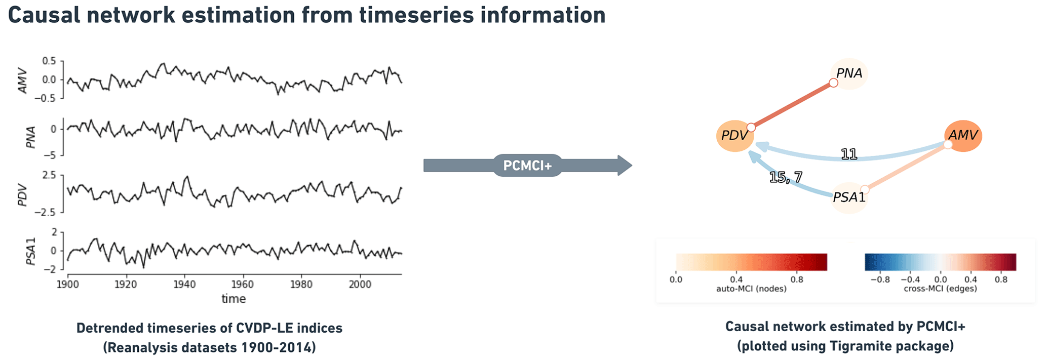
Figure 2 Constructing a causal network using Tigramite by applying PCMCI+ to time series calculated by CVDP-LE from reanalysis datasets. Each node on a causal network (right) represents a variable (time series, left), and the node color represents its auto-correlation (self links of each variable). The link color shows the cross-MCI partial correlation value which denotes the sign and strength of the estimated causal link between two variables. The time lag for lagged links (curved arrows) are shown as small labels on the links. Straight lines represent instantaneous causal links happening with no time lag.

Figure 2 demonstrates the application of the PCMCI+ algorithm to CVDP-LE datasets. Since causal discovery requires stationary time series (Runge, 2018), we first consider in our analysis the detrended yearly 1900–2014 time series of modes of climate variability, namely AMV, PNA, PDV and PSA1 (left). The resulting causal network from the application of the PCMCI+ algorithm is shown on the right (Fig. 2). The direction, sign, strength (|cross-MCI| value) and time lag (τ) of the estimated causal links are all attributes that can be conveniently read off the generated causal graphs. Each node on a causal network represents a variable, and the node color represents its auto-correlation (self-links of each variable). The link color shows the cross-MCI value which denotes the sign and strength of the estimated causal link between two variables. The time lag for lagged links (curved arrows) are shown as small labels on the links. For those connections that occur at multiple lags, the color of the link shows the strongest link, but the label depicts all significant lags sorted by their strength. The contemporaneous links are shown as straight arrows (“→” when directionality is decided), straight lines with circle-shaped ends (“∘–∘” when the adjacency indicates a Markov equivalence) or straight lines with cross-shaped ends (“x–x”, indicating conflicting orientation rules).

With regards to the parameter settings for the PCMCI+ algorithm, we set the maximum time lag (τ_max) to 15 years (τ_max=15 time steps, as we are using one data point per year). The significance level of the MCI partial correlation tests above α_pc is set to 0.05.

2.1.3 Setup for regime-oriented analysis

The teleconnections between the Pacific and Atlantic Ocean basins are suggested to follow different regimes depending on the decadal phases that the AMV and PDV go through (Meehl et al., 2021a). In order to clearly identify the time periods of each phase, we smooth the time series data by applying 11-year and 13-year low-pass filters to PDV and AMV, respectively. Figure 3a shows the observed detrended low-pass-filtered AMV and PDV time series used to specify the different phases and regimes for the masking before applying the PCMCI+ algorithm (the labeled regimes on the time series are only 3 out of the 10 we run the analysis over). First, running the analysis on the complete time period is intended to reveal the consistent causal dependencies throughout the complete historical time series (see Fig. 2). The resulting causal networks from the complete period do not, however, expose much information on the causal effects which change over shorter time periods depending on how the PDV and AMV vary during those phases. In order to identify these phase-dependent causal dependencies, we perform the analysis on multiple shorter periods (regimes) by selecting the time steps that represent either the positive (warm) or negative (cold) phases based on the low-pass-filtered indices, with AMV$+(-)$ for when the value of low-pass-filtered AMV is positive (negative); the same is the case for PDV$+(-)$. We further split these regimes into combinations of warm and cold PDV and AMV phases (PDV+/AMV+, PDV+/AMV−, PDV−/AMV+, PDV−/AMV−). Additionally, since some regimes are too short to reveal any dependencies, we also opted to run the analysis for an “in-phase” regime that sums the PDV+/AMV+ and PDV−/AMV− periods. The remaining time steps would then consist of the “out-of-phase” regime for the period where the two low-pass-filtered indices have opposite signs (PDV+/AMV− and PDV−/AMV+).

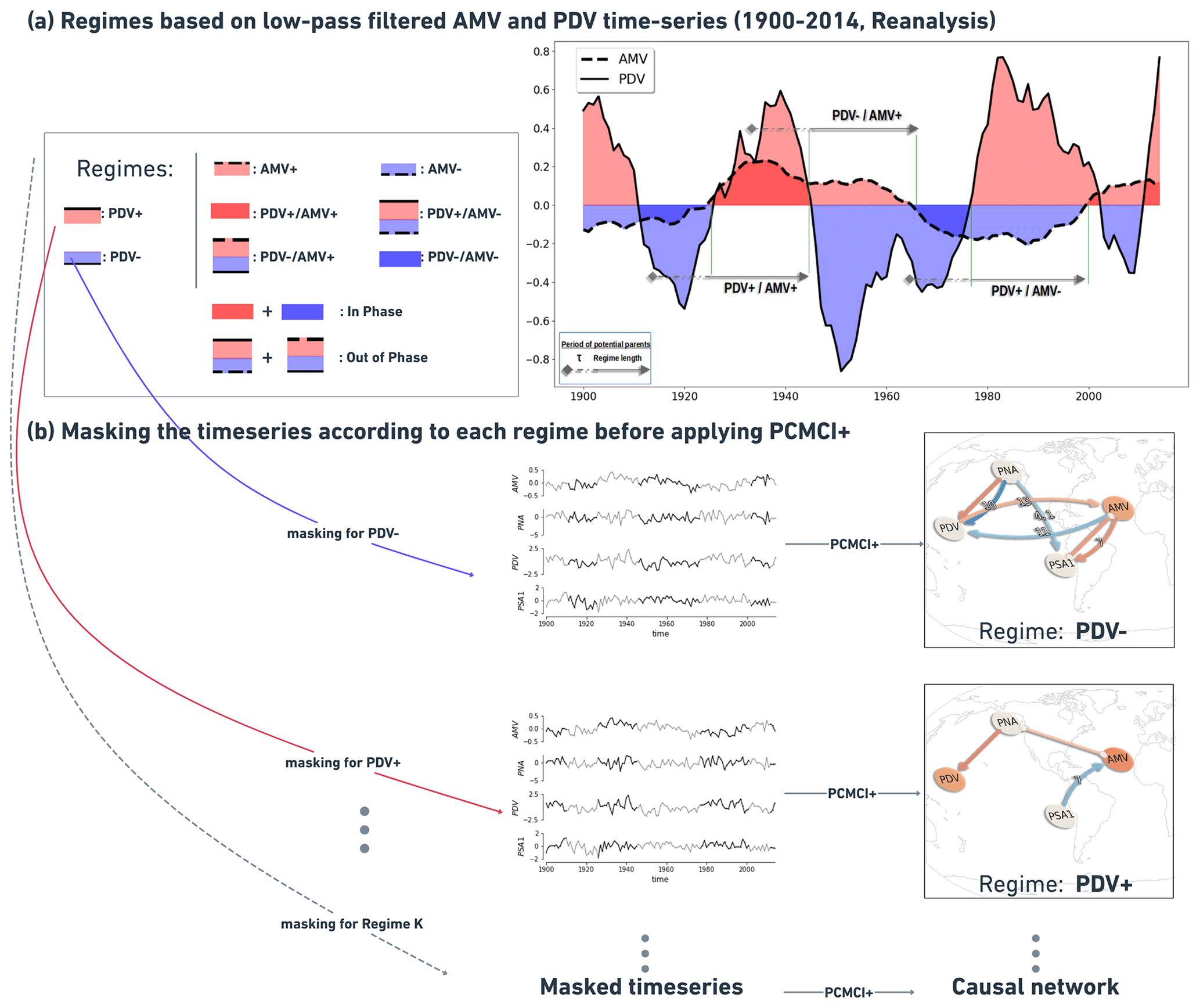
Figure 3 (a) PDV and AMV time series calculated by CVDP-LE diagnostics on ERSSTv5 data are smoothed using 11-year and 13-year low-pass filters, respectively. A total of 10 regimes are defined (see table on the left) in addition to the 1900–2014 complete period. The PCMCI+ algorithm is applied to unfiltered (non-smoothed) PDV, AMV, PNA and PSA1 yearly detrended time series that are masked according to the periods that define each regime. The right arrows on the smoothed time series represent unmasked periods from 3 out of 10 regimes (PDV+/AMV+, PDV−/AMV+ and PDV+/AMV−). (b) The regimes identified in (a) are used to mask the non-smoothed (but detrended) index time series before applying PCMCI+. Here, for example, we show how we mask the data according to the PDV− (top) and PDV+ (bottom) regimes. The gray shaded periods are masked and thus not considered during the PCMCI+ analysis. Note that the masking here refers to variables at time point $X_{\mathrm{t}}^j$, while their lagged parents can also originate from a masked period (gray shaded). This setting is referred to as mask_type='y' in Tigramite. Consequently, applying PCMCI+ to differently masked time series produces different causal networks (network in top vs. network in bottom)

This means that, in addition to running it on the complete period, we apply the PCMCI+ algorithm to 10 different shorter time periods (within the original 1900–2014 period) for each dataset (see Fig. 3a for reanalysis data). Figure 3b shows how we use the regimes defined in Fig. 3a to mask the time series before applying the PCMCI+ method. This is shown for PDV+ and PDV− regimes as examples. For each case, the gray-shaded parts of the time series are masked periods; i.e., only the black-shaded periods (see time series in Fig. 3b) are considered. We show in Tables A4 to A10 in the Appendix the number of years per regime for each dataset analyzed. Nonetheless, it should be stated that the results of the regime-oriented causal analysis account for potential errors related to the sampling of the data. A study from Smirnov and Bezruchko (2012) demonstrated, using a variety of examples, how sampling at lower intervals can produce large “spurious” results.

We note that the low-pass-filtered indices are used only to extract the time periods that constitute each regime. We remove any linear trend that might be present in the data prior to applying the causal discovery algorithm. In this way, the effects of external forcings are reduced. The four indices (AMV, PNA, PDV, PSA1) to which PCMCI+ is applied are represented by detrended yearly unfiltered (not smoothed) time series (see Figs. 2 and 3b).

2.1.4 F₁-scores for causal network comparison

To quantify the similarity between the resulting causal graphs (networks) from model simulations and those from observations, we follow a similar modified F₁ score as in the methods by Nowack et al. (2020). The F₁ score ranges between 0 (no match) and 1 (perfect network match) and is based purely on the existence or non-existence of links in a network relative to a reference network. The F₁ score combines the statistical precision (P, which is the fraction of links in the model simulation network that also occur in the reference network) and recall (R, which is fraction of links in the reference network that are detected in the model simulation network) and is defined as follows:

$$\begin{array}{}\text{(2)}& F_{\mathrm{1}}={\displaystyle \frac{\mathrm{2}\times P\times R}{P+R}},\end{array}$$

with

$$\begin{array}{}\text{(3)}& P={\displaystyle \frac{\mathrm{TP}}{\mathrm{TP}+FP}},\end{array}$$

and

$$\begin{array}{}\text{(4)}& R={\displaystyle \frac{\mathrm{TP}}{\mathrm{TP}+FN}},\end{array}$$

where FP is the number of falsely detected links, and FN is the number of undetected links. We modify the definition in the same way as Nowack et al. (2020) so that a link is considered to be a true positive (TP) if it is found with the same sign of MCI partial correlation as that in the reference network. We further relax the time lag constraint by considering a TP to exist if a link is found in a ±10 time step interval compared to the lag in the reference network (i.e., $min({\mathit{\tau }}_{\max },\mathit{\tau }+\mathrm{10}),max(\mathrm{0},\mathit{\tau }-\mathrm{10})$).

2.2 Data

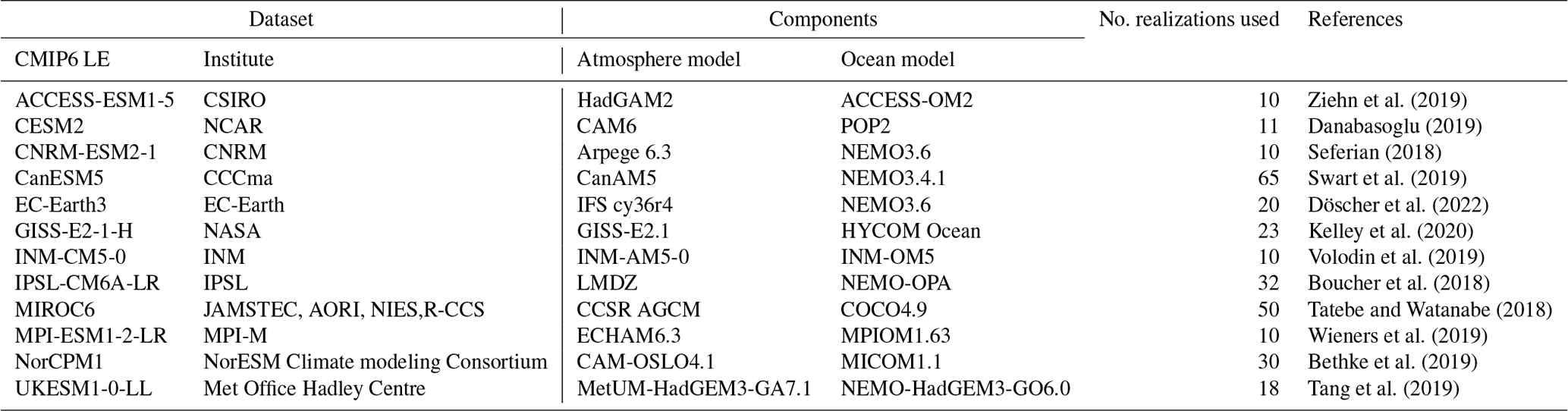
From the 1900–2014 historical climate variability diagnostic results provided by the CVDP-LE, we choose the SST from the Extended Reconstructed Sea Surface Temperature (ERSST) version 5 (Huang et al., 2017) of the National Oceanic and Atmospheric Administration (NOAA) as a reference for the AMV and PDV indices and spatial patterns. On the other hand, for the PNA and PSA1 modes, we use as a reference the SLP from the 20th Century Atmospheric Reanalysis extended with ERA5 (ERA20C_ERA5), provided by the European Centre for Medium-Range Weather Forecasts (ECMWF), and the assimilated observations of surface pressure. The reference data are for comparison to evaluate how indices generated using a selection of 12 large-ensemble CMIP6 historical models reproduce the observed spatial patterns and causal dependencies. The list of CMIP6 LE models (with the number of realizations per model) is provided in Table 1.

Ziehn et al. (2019)Danabasoglu (2019)Seferian (2018)Swart et al. (2019)Döscher et al. (2022)Kelley et al. (2020)Volodin et al. (2019)Boucher et al. (2018)Tatebe and Watanabe (2018)Wieners et al. (2019)Bethke et al. (2019)Tang et al. (2019)

Table 1 CMIP6 large-ensemble historical simulations used in the analysis.

We note that, in the spatial correlation analysis in the next section, monthly averages are used for AMV and PDV, as that is the time resolution originally provided by the CVDP-LE for these modes. The diagnostic package does not produce monthly fields for the PNA and PSA1, so we use winter means (DJF) and all-year annual means (ANN), respectively. We found that most model simulations show weak correlations with reanalysis data for the annually averaged PNA (ANN; not shown) compared to the winter-averaged PNA (DJF; Table 2). Hence, we chose winter means instead of annual means for PNA to reduce any seasonal bias within the simulated spatial patterns. The spatial patterns do not depend much on the time resolution (yearly or monthly) of the data, as they are all calculated from the whole 1900–2014 period. Prior to applying the causal discovery algorithm (Sect. 3.2), however, we yearly average the AMV and PDV time series (computed based on monthly means by the CVDP-LE). This way, we unify the time resolution of our data to fit the causal analysis by using the yearly resolution to investigate connections on long timescales.

3 Results

3.1 Similarities between the simulated and observed spatial patterns

To accompany the causal analysis, we first calculate pattern correlations (r) for each simulation's SST and SLP regression maps with respect to the reanalysis regression maps (for the complete 1900–2014 period, see Fig. 4a). This is to quantify the similarity between the observed and simulated spatial patterns for each of the four modes of climate variability we are to analyze. The purpose is to check if the CMIP6-simulated indices have spatial expressions that resemble those of indices calculated from reanalysis datasets. To introduce a benchmark of model performance, we calculate a mean score for each single simulation by taking the average of the four r values (after applying a Fisher z transform).

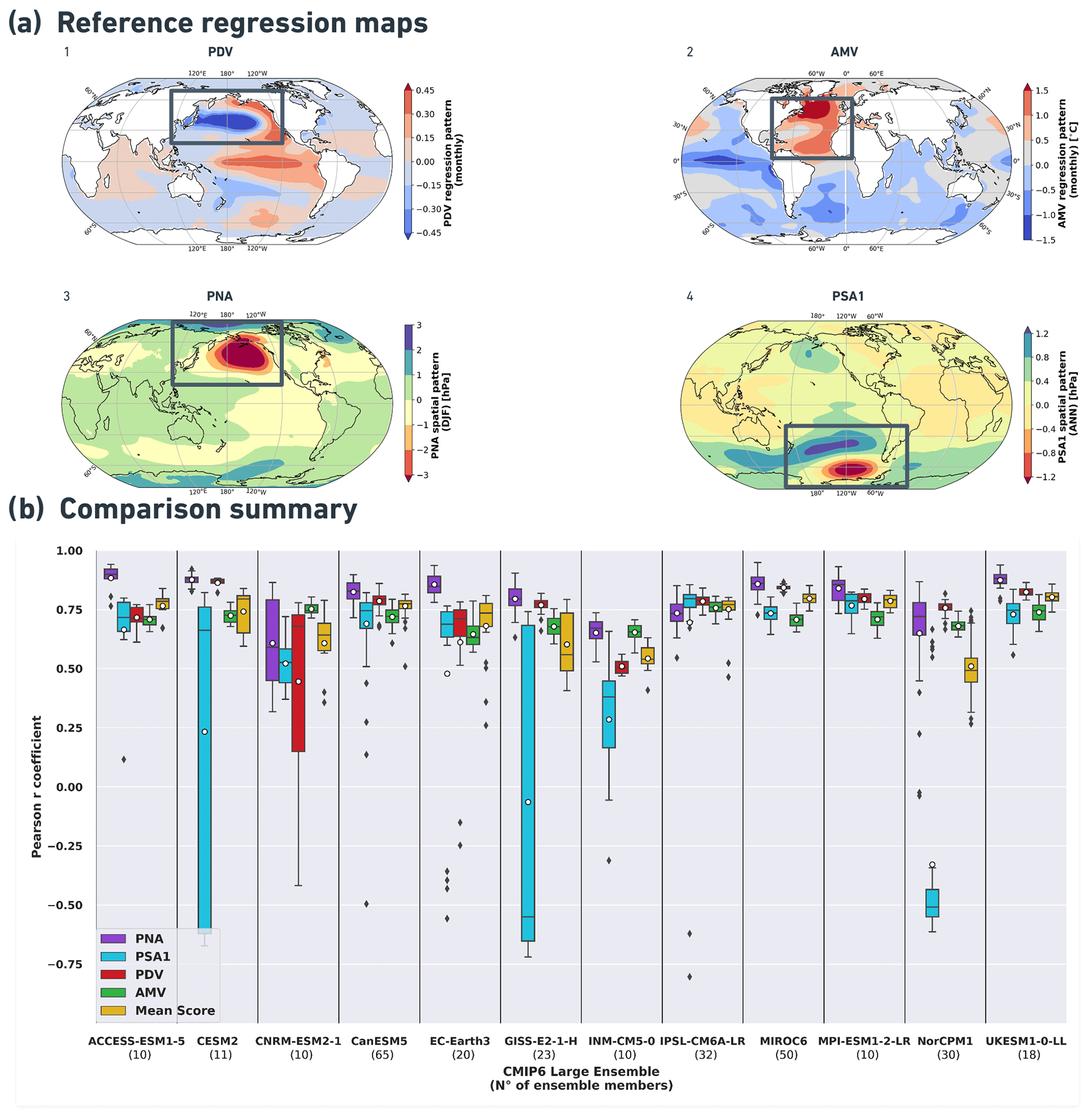
Figure 4 (a) Reference for comparison: SST regression maps showing geographical patterns associated with PDV (1) and AMV (2) and SLP regression maps of geographical patterns associated with PNA (3) and PSA1 (4). The indices are calculated from reanalysis data (ERSSTv5 for AMV and PDV, ERA20C_ERA5 for PNA and PSA1) over the 1900–2014 period using the NCAR CVDP-LE package. Rectangles on the maps approximate the regions over which the indices are defined (see Methods, Sect. 2.1.1). (b) Box plot (or whisker plot) showing the distribution of Pearson r pattern correlation values along the different historical CMIP6 LEs (between parenthesis on the x axis is the number of ensemble members within each model). The bottom of every box (color-coded part) shows the first quartile (Q₁ or 25th percentile), the top shows the third quartile (Q₃ or 75th percentile), and the horizontal bar between them denotes the median value (Q₂ or 50th percentile). The length of the box (from Q₁ to Q₃) denotes the interquartile range (IQR), while the bottom and upper whiskers (thin lines extending from boxes) extend to the minimum and maximum values, which are calculated as $Q_{\mathrm{1}}-\mathrm{1.5}\times$ IQR and $Q_{\mathrm{3}}+\mathrm{1.5}\times$ IQR, respectively. The black dots are outliers. PNA correlation values are shown in purple, PSA1 values are shown in cyan, PDV values are shown in red, and AMV values are shown in green. Yellow boxes show the mean score denoting the average of the four r values (after applying a Fischer z transform). White dots denote the mean value.

To look closer at how the spatial correlation values spread across every LE and how they differ from one climate variability mode to another, Fig. 4b provides a color-coded box plot showing the distribution of these spatial correlation values and their respective averages across every large ensemble of CMIP6 simulations used in the analysis. It depicts the similarity between the observed (reference maps in Fig. 4a) and the simulated patterns from the regression maps for the four modes, with values approaching 1 indicating a better simulation of the patterns associated with the observed modes.

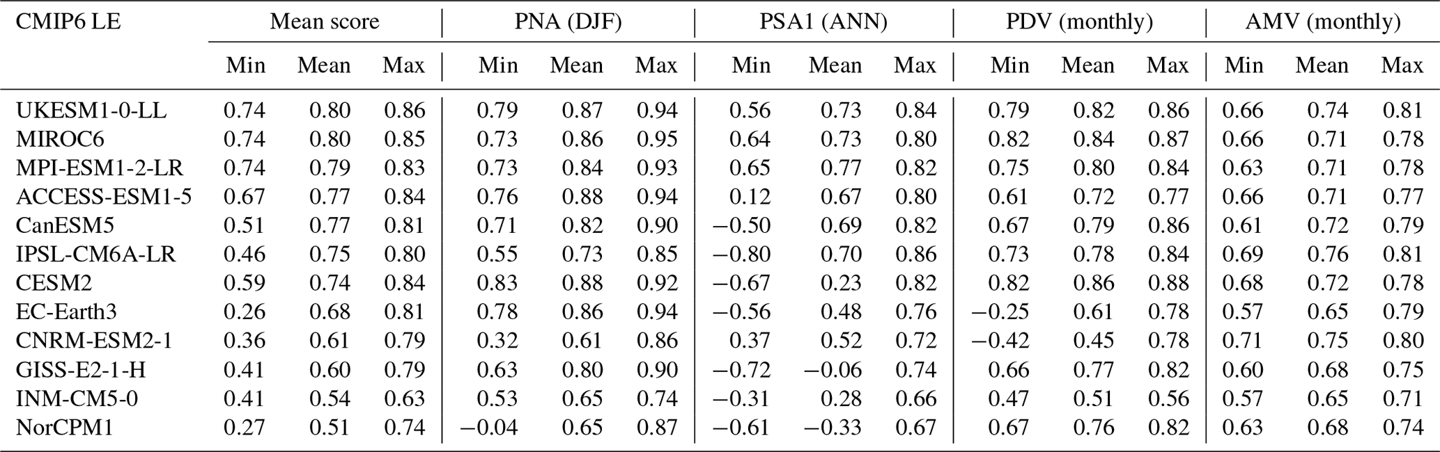
Sorted by the ensemble-average mean score of every CMIP6 LE, Table 2 provides a view of the distribution (in the form of minimum, mean and maximum) of the spatial correlation values for every mode and their mean score for every CMIP6 LE model. It can be seen from Fig. 4b and Table 2, based on the ensemble-average mean score, that most models perform quite well in simulating the observed geographical patterns of the four indices in Fig. 4a, with pattern correlations mostly above 0.75. The UKESM1-0-LL (0.80), MIROC6 (0.80), MPI-ESM1-2-LR (0.79), ACCESS-ESM1-5 (0.77) and CanESM5 (0.77) outperform the other CMIP6 LEs in terms of recreating the spatial patterns of the four selected modes of climate variability. The number of ensemble members within every LE has no apparent effect on the spread of the r value distribution across the models. For example, UKESM1-0-LL and MIROC6, with 18 and 50 realizations, respectively, share similar narrow interquartile ranges (IQR – the width between the third and first quartiles) of r values for the four climate variability spatial patterns. Table A1 in the Appendix shows the distribution of Pearson r correlations between observed and simulated spatial patterns of PNA, PSA1, PDV and AMV from a 10th-, 50th- and 90th-percentile perspective. Looking only at the mean-score spread, Table A1 shows that the 10th–90th percentile value range is 0.78–0.83 for UKESM1-0-LL and 0.77–0.82 for MIROC6. This means that most members of these two model ensembles agree with each other and show high spatial similarity with observations when simulating the four modes. It can be concluded that the models generally do a good job in simulating the geographical patterns of the different modes but with different precision. Although the models with high mean scores tend to display high pattern correlations with observations for the four modes of climate variability, the white scatter points in Fig. 4b imply that they simulate the PNA (purple) atmospheric mode slightly better than its South Pacific counterpart, the PSA1 (cyan), when compared to the ERA20C_ERA5 reference patterns. These high-scoring models, notably UKESM1-0-LL, MPI-ESM1-2-LR, MIROC6, CanESM5 and IPSL-CM6A-LR also, on average, simulate better PDV (red) monthly spatial patterns compared to those of AMV (green) with ERSSTv5 as a reference dataset for the 1900–2014 period. The mean scores of CESM2, GISS-E2-1-H and NorCPM1 are strongly affected by the low correlation coefficients obtained for the PSA1 mode (cyan boxes). The 50th percentile bar on the cyan box for CESM2 suggests that there are more members with PSA1 patterns that resemble the observed ones. The opposite is true for the GISS-E2-1-H model, which contains fewer realizations with PSA1 patterns similar to those from reanalysis. The length of the cyan box for NorCPM1 indicates that most members fail to represent the spatial patterns of PSA1.

Table 2 Pearson r correlations between the simulated (CMIP6 LE) and observed (ERA20C_ERA5, ERSSTv5) spatial patterns of PNA, PSA1, PDV and AMV over the 1900–2014 period. Models are sorted according to the average mean score (column in bold; descending order).

Along with the release of the CVDP-LE (Phillips et al., 2020), CESM's CVCWG freely distributes results from several CMIP simulations, including the CMIP6 1900–2014 historical simulations, from which data used in this analysis have been downloaded. The results include a pattern correlation summary with 11 key spatial metrics of oceanic and atmospheric modes of variability. Similar to the mean score we introduced in the spatial correlation analysis above, the CVDP-LE provides a mean score that averages the pattern correlations of the 11 metrics used. Although the pattern correlation mean score we calculated is not exactly the same as the one provided by the CVDP-LE tool because the number of indices used is different (4 vs. 11), the highest-scoring CMIP6 LEs from Table 2 (UKESM1-0-LL, MIROC6 and MPI-ESM1-2-LR) were also the highest-scoring ensembles according to the pattern correlation summary provided on the tool's repository (Phillips et al., 2020). Moreover, one simulation from the UKESM1-0-LL ensemble, the r19i1p1f2 realization, was found to obtain the highest mean score based on both the pattern correlation values published under https://webext.cgd.ucar.edu/Multi-Case/CVDP-LE_repository/CMIP6_Historical_1900-2014/metrics.html, last access: 17 March 2023, by CVDP-LE authors (Phillips et al., 2020, 0.88 using 11 indices) and our calculations in Table A2 (0.86 using 4 indices)

3.2 Regime-oriented causal analysis of observations and reanalyses

Several mechanisms are hypothesized to contribute to PDV and AMV. PDV is initially considered to be a mode of internal climate variability (e.g., Meehl et al., 2021b). However, previous research indicates possible external contributions in the form of solar (Meehl et al., 2009), greenhouse gas (Meehl et al., 2009; Fang et al., 2014; Dong et al., 2014) or volcanic and anthropogenic aerosol forcings (Wang et al., 2012; Maher et al., 2015; Smith et al., 2016; Takahashi and Watanabe, 2016). There are studies suggesting that such external anthropogenic aerosol forcing might be a contributor to AMV as well (Booth et al., 2012; Zhang et al., 2013; Si and Hu, 2017), but evidence from Zhang et al. (2019) supports the notion that the AMV is primarily linked to internal variability of the Atlantic meridional overturning circulation (AMOC) and its associated meridional heat transport. This means that the fingerprint of any possible external forcing acting as a confounder is embedded in the time series information of the extracted indices of the modes of climate variability used in this study. The linear detrending we perform prior to applying PCMCI+ will at least partially reduce such effects. However, as mentioned before, the subtraction of the global mean temperature for PDV and AMV and the linear detrending of all time series do not address local, nonlinear effects, which could be related to the aerosol forcing that varies over time and space. It is then important to recall that, in this paper, the indices do not represent a fully isolated internal variability component but rather a mixture of naturally occurring internal variability and nonlinear effects of external forcing, mainly in the form of aerosol forcing.

PCMCI+ is applied first to the indices of PDV, AMV, PNA and PSA1 that were calculated from reanalysis data as a proxy for observations in order to reveal any causal dependencies between the modes depicted by the observed time series information. As it is assumed that the nature of teleconnections between the different climate variability modes can vary over decadal timescales depending on the different phases these modes go through, we mask years of data (as discussed in Sect. 2.1.3) to reveal the causal structures during specific periods (regimes) in time. Reference causal networks obtained by running PCMCI+ on reanalysis data for the different regimes are shown in Fig. 5.

The results show that the causal dependencies (links) between the four modes of climate variability (nodes) change from one regime to another. Starting from an analysis of the complete-period (115 years; upper left panel in Fig. 5; see also Table A3 for exact cross-MCI values of the complete-period causal graph) PCMCI+ reveals four different links: an 11-year-lagged negative (link arrow is curved and blue) AMV → PDV link (cross-MCI $=-\mathrm{0.25}$) showing that the opposite-sign effect on PDV caused by AMV is lagged by a decade (e.g., positive AMV tends to produce negative PDV about a decade later). Therefore, this link can be interpreted as lagged opposite-sign SST anomaly changes over the Pacific in response to SST anomaly changes over the Atlantic. The same causal graph features a strong positive (0.53) contemporaneous PDV–PNA link (i.e., link line is straight), suggesting that PDV is strongly associated with PNA. In addition, the complete-period graph implies weak South Pacific teleconnections of both AMV and PDV, which are represented by a positive contemporaneous AMV–PSA1 (0.25) link and a lagged PSA1 → PDV link. The latter (PSA1 → PDV link) is detected as positive at 7 years (0.23) and as negative at 15 years (−0.31). As explained in Sect. 2.1.2, if a lagged link is found at more than one time lag, the causal graph shows the link at the lag when it is most significant (i.e higher absolute cross-MCI value) and labels the other time lags after causal links due the lack of a comma ($|-\mathrm{0.31}|$ vs. $\left|\mathrm{0.23}\right|$ in this case, hence the “15, 7” label on the PSA1 → PDV link; see upper left panel in Fig. 5).

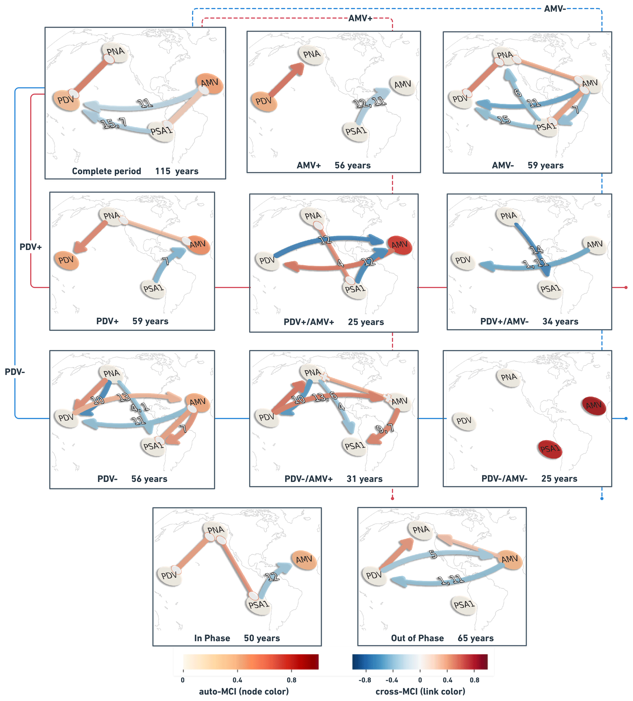
Figure 5 Causal networks calculated with PCMCI+ from reanalysis data for the complete 1900–2014 period (upper left panel) and the different regimes. Nodes represent the time series associated with each climate variability index (see node labels) masked according to the predefined regimes. Node colors indicate the level of autocorrelation (auto-MCI) as the self-links of each node, with darker red indicating stronger autocorrelations (color bar, lower left), while the color of the arrows (termed “links” here) denotes the inter-dependency strength (cross-MCI), with blue indicating opposite-sign (or negative) inter-dependency and red indicating same-sign (or positive) inter-dependency strength (color bar, lower right). Small labels on the curved links indicate the link-associated time lags (unit =1 year). Straight links show contemporaneous inter-dependencies that happen with no time lag (i.e., τ<1). Each network is sub-labeled with its respective regime name and the total number of unmasked years (time steps) that characterize that regime (label and number of years at the bottom of each panel). Lines going through the panels are to help visualize which combinations make up the regimes. Solid lines are for PDV, and dashed lines are for AMV. Red is for warm (+) phases, and blue is for cold (−) phases (e.g., PDV+/AMV− regime panel has a solid red line and a dashed blue line going through it).

The complete-period graph in the upper left in Fig. 5 is useful to show the causal dependencies happening throughout the whole observational record used. However, this methodology can also be used to look at specific regimes to notice the change in dependencies arising from the physical state of the Atlantic and Pacific basins during those time periods. For example, the causal graphs from PDV+ and PDV− regimes indicate that direct decadal AMV–PDV interactions occur only during the PDV− regime (third row, left panel in Fig. 5), whereas during the PDV+ regime (second row, left panel in Fig. 5), we find a contemporaneous atmospheric teleconnection from PNA to both AMV and PDV. This difference could be explained by the fact that the PDV− regime comprises two important Atlantic variability events: the 1920s AMV phase switch from negative to positive (see dashed lines showing low-pass AMV in Fig. 3a) and the subsequent switch from positive back to negative during the late 1960s.

The regime-oriented nature of this causal analysis provides for a separation of signals – for example, delineating the PDV+ regime that depends on the AMV phase during those 59 years (second-row panels in Fig. 5). The short length of the time series, in addition to the time-varying aerosol forcing during such regimes, can lead to inconclusive causal estimations. The PDV−/AMV− panel at the right of the third row in Fig. 5 (25 years) shows strongly auto-correlated AMV and PSA1 patterns but no apparent links between any of the four variables. However, these short regimes might also reveal interesting causal relations that are not apparent when analyzing longer periods. This is the case for the causal graph from the 25 years of the PDV+/AMV+ regime (central panel in Fig. 5), which is the only one to feature a strong negative PDV → AMV link and a positive AMV → PDV link with comparable strength. Since the causal parents that drive the variables (other variables or the same one at different past time steps) can originate from a masked period with respect to τ_max, it implies, for example, that the strong 12-year-lagged negative PDV → AMV causal link estimated during the PDV+/AMV+ regime (second row, central panel in Fig. 5) might have fingerprints that originate from a previous regime.

The limitation presented by the fact that some regimes might be too short to detect any causal links (e.g., PDV−/AMV−, 25 years) is overcome when introducing causal graphs for in-phase and out-of-phase regimes (panels in the bottom of Fig. 5). As explained in Sect. 2.1.3, the in-phase regime is made up of the time steps where AMV and PDV happen to be on the same phase (PDV+/AMV+ and PDV−/AMV−), while the out-of-phase regime is composed of time steps where the two modes are on opposite phases (PDV+/AMV− and PDV−/AMV+), resulting in longer regime periods. We detect the negative lagged direct AMV → PDV and PDV → AMV only during the out-of-phase regime, with a strong positive, extra-tropical PDV → PNA teleconnection and a weaker AMV → PNA teleconnection. The in-phase regime features a fast (zero-lag) PDV teleconnection to PNA, a PNA connection to PSA1, and a 12-year-lagged PSA1 → AMV link. As finite sample errors can lead to false positives and also false negatives (missing links), it is difficult to attribute a physical explanation to every detected link. Although, here, both are thought to be driven by tropical precipitation and heating anomalies, we refrain from assigning any processes that might be behind the direct PNA–PSA1 causal links due the lack of knowledge regarding possible direct links between the North Pacific and South Pacific extra-tropics.

Through observations of the long-term variability patterns and pacemaker simulations of Atlantic and Pacific Ocean basins, Meehl et al. (2021a) explain how positive AMV could produce an opposite-sign response, mainly through the atmospheric Walker circulation, leading to negative PDV and then to the negative PDV subsequently contributing a same-sign response in the Atlantic, driving the AMV from positive to negative phase. This mutual contrasting response from one basin to the other can be interpreted through the blue (negative cross-MCI) lagged AMV → PDV links and the reddish (positive cross-MCI) lagged PDV → AMV links in the causal networks in Fig. 5. The results in Fig. 5 show that the lagged AMV → PDV causal link has been estimated over the complete period and during 5 out of the 10 regimes (AMV−, PDV−, PDV+/AMV+, PDV+/AMV− and out-of-phase). During four of these regimes, the link can be interpreted as a lagged opposite-sign effect of AMV on PDV (curved blue link). The study of Meehl et al. (2021a) suggests that, in addition to the tropical Walker circulation, positive convective heating and precipitation anomalies in the tropical Pacific establish extra-tropical teleconnections to PNA and PSA, which contribute to the same-sign effect of PDV on AMV. The causal graph from the 31 years of the PDV−/AMV+ regime (third row, middle panel in Fig. 5) shows two possible pathways for this same-sign effect of PDV on AMV. During that regime, PCMCI+ estimates a strong positive 13- and 6-year-lagged PDV → AMV link (the 13-year-lagged link was also found during the 56 years of the PDV− regime) but also shows a positive PDV → PNA–AMV contemporaneous teleconnection where PNA seems to mediate the same-sign effect of PDV on AMV. Therefore, this analysis presents additional evidence that AMV (although potentially affected by a forced aerosol signal) might serve as a predictor of decadal variability over the Pacific (hence for PDV) and, eventually, the other way around (d'Orgeville and Peltier, 2007; Zhang and Delworth, 2007; Chikamoto et al., 2015; Johnson et al., 2020).

An earlier study from Zhang and Delworth (2007) proposed a mechanism in which positive (negative) AMO would lead to high (low) SLP anomalies over the North Pacific and eventually to a positive (negative) PNA pattern. This weakening (strengthening) of the Aleutian low associated with the PNA pattern projects onto the multidecadal mode of variability over the North Pacific. The response of North Pacific SST to the anomalous PNA pattern induced by AMO is hypothesized to be lagged due to Rossby wave propagation and gyre adjustment; in this regard, the authors found a 3-year lag when using a model simulation compared to a 12-year lag when they analyzed the observed pattern. The extra-tropical contributions of PNA and PSA1 to the mutual PDV–AMV interactions can be concluded from causal graphs constructed during different regimes (see Fig. 5). AMV−, PDV+, PDV−/AMV+ and out-of-phase are all regimes that suggest that mutual Atlantic–Pacific connections can be established via PNA. The causal networks from the complete period and AMV− regime show that these inter-basin connections can also happen through PSA1.

Previous research also showed that components of the PDV can be forced by tropical Pacific variability and/or driven by atmospheric stochastic forcing, which are both closely tied to Aleutian low variability associated with the PNA pattern (Newman et al., 2016; Johnson et al., 2020). This finding in the literature regarding the PDV–PNA teleconnection validates the contemporaneous PDV–PNA causal link estimated by PCMCI+ during most regimes (all except PDV+/AMV+ and PDV−/AMV−; see causal networks in Fig. 5) with a strong positive cross-MCI value. The link is directed in some regimes (straight links with arrowhead, e.g., during PDV+ regime), while it is unoriented during other regimes (straight links with no arrowheads, e.g., during AMV− regime). A 10-year-lagged negative PNA → PDV link appears during the PDV− regime in Fig. 5 (and during PDV−/AMV+), which suggests that an extra-tropical teleconnection to PNA might have the opposite effect during longer time lags.

Generally, lags ranging from interannual (1 to 5 years;  Wu et al., 2011; Meehl et al., 2021a) to decadal (12 to 17 years; Wu et al., 2011; Chylek et al., 2014) timescales have been proposed by previous studies for Atlantic–Pacific interactions; these fall in the same range of time lags at which causal links have been estimated by PCMCI+ in this study.

To further justify the credibility of the constructed causal networks, we use the estimated causal graph from the complete period to construct a model that explains the lagged correlation structure of the reanalysis dataset. This is done by fitting a linear structural causal model to causal parents taken from the original reanalysis causal graph. We generate 100 realizations following a linear Gaussian causal model, with the noise structure estimated from the noise covariance matrix of residuals. Fig. 6 shows lagged correlations of the original data in red, with the mean lagged correlations from the synthetically generated data in black and their 5th–95th percentile range in gray. The original lagged correlations (red) fall mostly within the 90 % range (with the clear exception of AMV's lagged auto-correlation at the upper left of Fig. 6). This means that a linear Gaussian model with the same links as those from the reconstructed causal graph can explain well the whole lagged-correlation structure of the original data for PNA, PDV and PSA1. Such a lagged-correlation matrix (Fig. 6) also unveils how the dependencies between different variables change over time.

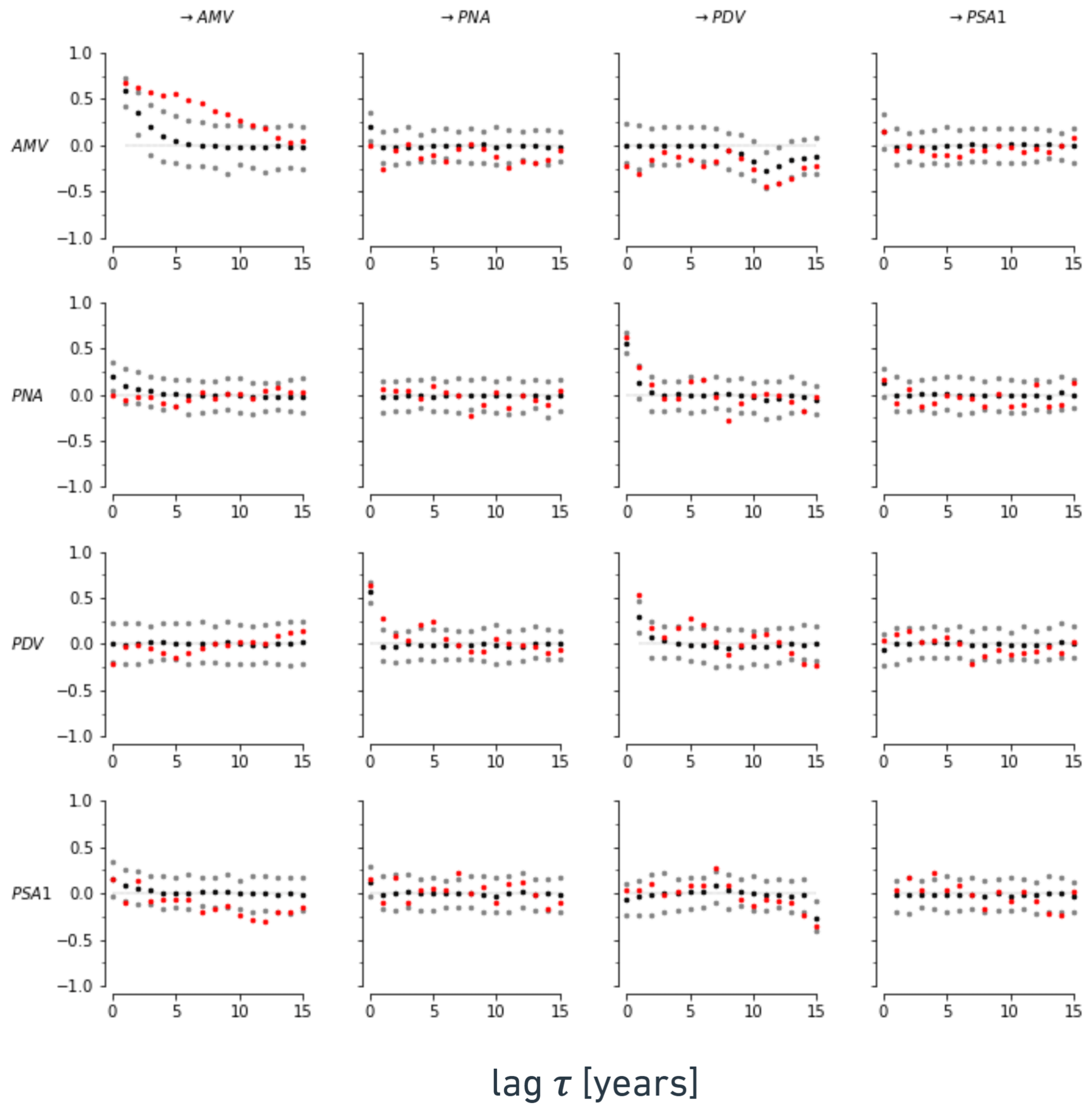
Figure 6 Lagged correlations of original data (lag in years; complete-period graph from reanalysis data) in red, shown together with lagged correlations of an ensemble of synthetic data generated by a linear Gaussian structural causal model, with causal coefficients and noise structure estimated from the original data. The mean lagged correlations from the synthetically generated data are shown in black, and their 5th–95th percentile ranges are shown in gray. The x axis shows lag in years.

3.3 Regime-oriented causal model evaluation of the CMIP6 large ensembles

With the overall high level of fidelity that several models show in simulating the spatial patterns of at least the major modes of climate variability presented in this paper (see Fig. 4b), it is crucial to test whether these simulations also account for the possible lagged causal pathways between these different modes. To benchmark the dependency structures in model simulations, the simulated causal graphs are compared to those from reanalysis datasets (ERSSTv5 for PDV and AMV, ERA20C_ERA5 for PNA and PSA1). The constructed causal graphs from the previous section illustrate the connections that occur between the different modes of climate variability during different regimes, as estimated from reanalysis data. Relative to reanalysis, we consider the causal graphs from Fig. 5 as a reference for the CMIP6 model evaluation to be demonstrated in this section.

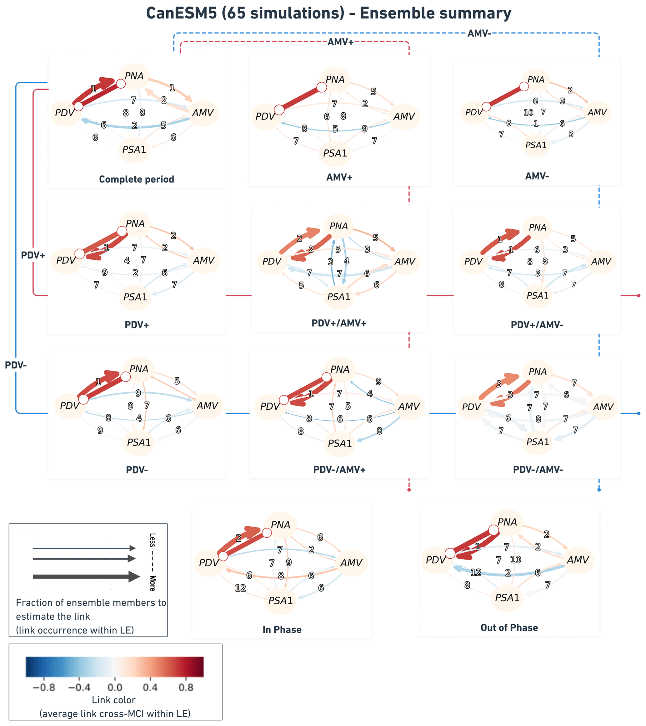
Figure 7 Ensemble summary of the CanESM5 LE model. Similar to Fig. 5 but aggregating causal networks from 65 realizations. The link width here shows the fraction of ensemble members that feature that link the relative to the total ensemble size (here, 65); i.e., the thicker the link, the more ensemble members were found to estimate it during that specific regime. Link colors here translate the mean cross-MCI value among the ensemble members that estimated such a link (color bar on the lower left). Links of very light color are those on which ensemble members show little agreement regarding their partial-correlation sign. The link labels indicate the average time lag (rounded to the nearest integer) at which the link is estimated among the fraction of ensemble members that find such a link.

The exact same PCMCI+ setting (see Methods; Sect. 2.1.2 and Sect. 2.1.3) used in the section above is applied for time series indices calculated from every realization of the CMIP6 models listed in Table 1. In Sect. 3.1, we found that, overall, the spatial patterns of these simulated indices compare fairly well to the observed ones (Fig. 4; Table 1). The purpose of this section is to show how the causal fingerprints in these simulations compare to those observed. For every realization, the analysis is run for the complete period in addition to the 10 different regimes, similarly to the regime-oriented setting on reanalysis data in the section above. As the PDV and AMV phases occur in model simulations at time periods that are different to those in reanalysis (due to randomly generated internal variability and time-varying forcing caused mainly by aerosols), models need not show similar networks for the same periods as those in observations. However, we can assess the degree of similarity in the causal fingerprints that these simulations hold within their modeled dynamics. The results of every realization during every regime are compared to the reference networks from reanalysis data during that regime.

To illustrate results from an individual model, we aggregate causal networks from 65 realizations from the CanESM5 model in Fig. 7. This figure shows networks with links of variable thickness, indicating that some links are found in most ensemble members during that specific regime (thick links, e.g., PDV–PNA in most regimes) compared to other links (thinner links, e.g., PDV → AMV in most regimes) which were detected by a only small fraction of ensemble members. The thicker the link, the more agreement between members of the same ensemble in detecting that specific link. We also label the links with the rounded mean lag at which they are detected in the ensemble members. The link color in this ensemble summary (Fig. 7) is informative regarding the level of agreement between ensemble members in estimating that causal link with the same sign. The clearer the shade of blue (negative) or red (positive), the better the agreement between ensemble members in simulating the link with the same sign. For example, the color of AMV–PNA links in most regimes (although mostly estimated by only a few members during each regime, i.e., relatively thin links; see Fig. 7) tends towards reddish shades, suggesting that the CanESM5 members, by which such links were estimated, agree that the causal link is of positive sign. This can be translated to the positive (negative) AMV driving positive (negative) PNA and vice versa. This can be seen in all causal networks in Fig. 7, except in the ones from PDV+/AMV+ and PDV−/AMV+ regimes, indicating that, in a few of the CanESM5 realizations, AMV would induce an opposite-sign response in PNA (see thin blue AMV → PNA links on PDV+/AMV+ and PDV−/AMV+ causal graphs in Fig. 7).

Other than the PDV–PNA links (estimated by most ensemble members during all regimes), the occurrence of a link in the CanESM5 model seems to vary from one regime to another. This is less true for the complete period and for the in-phase and the out-of-phase regimes. The complete-period ensemble causal graph distinctly shows AMV–PNA interactions as same-sign causal links between the two modes. The same graph (upper left panel in Fig. 7) also shows a clear blue AMV → PDV link, demonstrating the opposite-sign response driven by AMV in PDV, similar to the one featuring in the complete period causal graph from reanalysis data (upper left in Fig. 5). The color and width (thickness) of this AMV → PDV link in the complete-period graph in Fig. 7 (upper left panel) suggest that the link was estimated with negative cross-MCI values by a considerable fraction of CanESM5 simulations.

A more evident network similarity is evinced during the out-of-phase regime. Both the graph from reanalysis (Fig. 5, out-of-phase) and the CanESM5 ensemble graph (Fig. 7, out-of-phase) display a short-lagged (1-year lag and 2-year mean lag, respectively) opposite-sign (blue, negative cross-MCI) AMV → PDV causal link. Moreover, the two graphs (out-of-phase causal networks in Figs. 5 and 7) suggest same-sign (red, positive cross-MCI value) contemporaneous and short-lagged (1 year) PDV–PNA causal links and weaker same-sign (lower positive cross-MCI values) AMV–PNA links. The latter links are instantaneous in the reanalysis data but lagged in CanESM5. However, the short mean lag (2 years) in the simulated CanESM5 out-of-phase graphs implies that several members estimate a contemporaneous link.

The CanESM5 ensemble causal graph during the in-phase regime at the bottom of Fig. 7 demonstrates the advantage of using LEs. While the reanalysis graph during this regime suggests only PDV–PNA and lagged PSA1 → AMV teleconnections (with a debatable contemporaneous PNA–PSA1 link), the CanESM5 ensemble graph displays a clear same-sign lagged AMV → PDV link, with a third of its ensemble members simulating such a dependency. Despite the fact that the positive AMV → PDV link is not detected in reanalysis during the in-phase regime (Fig. 5, in-phase-regime causal graph), the literature supports this contrasting effect estimated by CanESM5 model data (Wu et al., 2011; Meehl et al., 2021a). Model simulations can therefore explain causal dynamics between modes of climate variability that might not definitively appear when analyzing observations. There is less doubt about the agreement between members of the CanESM5 ensemble and, when compared to reanalysis, about the occurrence of an AMV → PDV link with an opposite sign during the out-of-phase regime.

Ensemble summary plots are calculated for all CMIP6 LEs from Table 1, but we only chose to display them for CanESM5 in Fig. 7. The ensemble summary of causal networks from reanalysis data and the 12 CMIP6 models for the complete 1900–2014 period and for the out-of-phase and in-phase regimes are shown in Figs. A1–A3 in the Appendix, respectively. In order to measure the level of similarity between observed and individual ensemble member networks across all the CMIP6 models, F₁ scores are computed for every realization and every regime. The results reveal that most CMIP6 large ensembles show better network (causal graph) similarity with reanalysis reference networks during the out-of-phase regime compared to the networks drawn during the other regimes and/or the complete period. The whisker plot in Fig. 8a shows the distribution of F₁ scores across the CMIP6 LEs for the complete period (light-blue boxes), the in-phase regime (dark blue) and the out-of-phase regime (green). The range of scores during the other regimes (not shown) was found to be much lower compared to the scores during the regimes shown in Fig. 8a. The white scatter points show that, on average, CESM2, CanESM5, MIROC6 and MPI-ESM1-2-LR LEs clearly display better network similarity with observations during the out-of-phase regime. The highest scores during this regime (0.92) belong to members of CanESM5 and MIROC6 LEs (see location markers on whisker plot). Figure 8b compares out-of-phase causal graphs from these highest-scoring realizations (and their low-pass-filtered AMV and PDV time series) to those from reanalysis. The networks in Fig. 8b agree on the 1-year-lagged AMV → PDV link. The positive contemporaneous PDV–PNA link is directed differently in reanalysis and CanESM5 r11i1p2f1, but it is unoriented in CanESM5 r17i1p2f1 and MIROC6 r20i1p1f1. The out-of-phase graphs from these realizations also agree on a same-sign contemporaneous AMV–PNA dependency, with a lower (i.e., weaker) cross-MCI value than that of the PDV–PNA connection.

Figure 8 (a) Whisker plot showing the distribution of F₁ scores across the CMIP6 LEs for the causal analysis for the complete period (light-blue boxes), the in-phase regime (dark-blue boxes) and the out-of-phase regime (green boxes). White scatter points denote the mean LE F₁ scores. (b) Reference causal network estimated from reanalysis during the out-of-phase regime (left, with low-pass AMV and PDV time series below) compared to networks and time series from three CMIP6 simulations (right, with simulated low-pass AMV and PDV time series below each network) with the best network similarity, i.e., the highest F₁ score.

In Fig. 9, we perform intra- and cross-model network comparisons for the complete period and long regimes. This is done by computing F₁ scores with every single realization as a reference. Averaging the F₁ scores by ensemble produces an F₁ matrix for every regime in the form of heat maps that translate the degree of similarity (the redder the color, the greater the similarity) in causal dynamics between members of the same LE (boxes on the main diagonal) and the pairwise causal similarity between different LEs (boxes outside the main diagonal). Every grid box on the heat maps shows how the corresponding CMIP6 model from the axis on top (see model names on x axis top of every panel) compares to the reference corresponding CMIP6 model (see model names on y axis left of each panel). We exclude the short regimes (PDV+/AMV+, PDV+/AMV−, PDV−/AMV+ and PDV−/AMV−) from this comparison, as the PCMCI+ results during these regimes tend to be inconclusive (i.e., the regimes are too short to estimate any causal link for several simulations from different models). The heat maps show that CNRM-ESM2-1 LE clearly stands out as the most dissimilar model during most regimes. This is seen in the third row and third column (from top to bottom and from left to right) of each heat map (F₁ matrix of every regime) in Fig. 9, which indicates the lowest F₁ scores (yellow and white lines on the heat maps; see also the color bar). The model does not only have the lowest level of agreement with other ensembles but also shows poor accordance within its own members. Generally, the other CMIP6 models exhibit better network similarity during longer regimes (complete period, AMV+, AMV−, PDV+, PDV−, in-phase and out-of-phase). Members of CESM2 LE strongly agree with each other in terms of causal fingerprints displayed during the analysis over the complete period; this is shown by the dark-red box in the second row and second column of the complete-period heat map (F₁ matrix). The INM-CM5-0 LE shows low average F₁ scores during the PDV+ and out-of-phase regimes, but it surprisingly shows the most agreement between its own ensemble realizations during the complete period, AMV−, PDV− and the in-phase regimes (see dark-red grid boxes in the center of the heat maps of these regimes in Fig. 9). This implies that the INM-CM5-0 ensemble might mostly involve simulations where PDV and AMV are in the same phase.

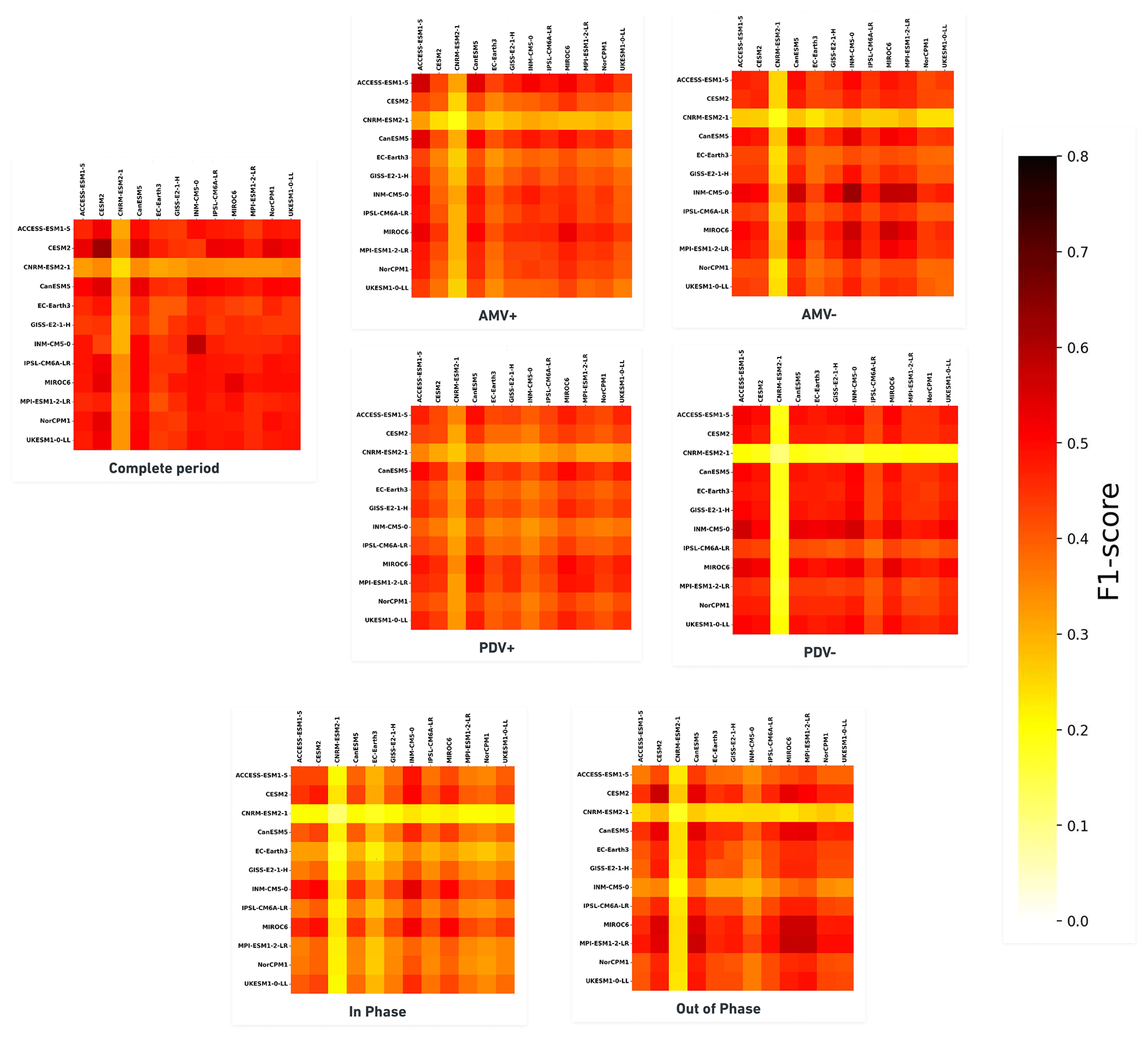
Figure 9 Matrices of average F₁ scores for pairwise network comparisons between ensemble members of 12 CMIP6 LEs during every regime. Boxes on the main diagonal translate the level of similarity between members of a single CMIP6 ensemble. Boxes outside the main diagonal show the similarity between realizations of a CMIP6 LE compared to realizations from another CMIP6 LE (taking every realization as a reference at a time before averaging across every LE). The redder the grid box, the better the causal network similarity it translates when comparing realizations of the corresponding CMIP6 model (x axis coordinate name on top of each panel) to causal networks from the corresponding reference CMIP6 model (y axis coordinate on the left of each panel). The matrices for the short regimes (PDV+/AMV+, PDV+/AMV−, PDV−/AMV+ and PDV−/AMV−) are not shown, as their results are not conclusive, since PCMCI+ fails to estimate any causal networks for several members of different ensembles.

The skill of CESM2, CanESM5, MIROC6 and MPI-ESM1-2-LR in recreating the observed causal pathways of the out-of-phase regime is also manifested through the better similarity the members of these models show when compared to each other. The heat maps (F₁ matrices in Fig. 9) serve to distinguish models with similar causal dynamics. The specified range of internal variability within realizations of the same ensemble (combined with the model-simulated time-varying aerosol forcing) can also be inferred by comparing one LE to itself.

3.4 Discussion

Previous research already suggested the improvement in the simulation of dominant modes of climate variability throughout the different phases of the CMIP archive (Fasullo et al., 2020; Eyring et al., 2021). Although, in general, models are able to capture the spatial patterns of these modes, CMIP6 revealed discrepancies in the skill these LE simulations display when recreating the observed modes. Some models perform very well, while there is still room for improvement for others. This conclusion is illustrated through the results of the pattern correlations in Sect. 3.1 and the wide range of comparison metrics produced and published by the CVDP-LE authors (Phillips et al., 2020). The ability of CMIP6 LEs to recreate the spatial patterns of modes of climate variability does not, however, ensure that they simulate the connections between those modes. Relative to the reference networks from reanalysis datasets during the out-of-phase regime, CESM2, CanESM5, MIROC6 and MPI-ESM1-2-LR LEs display the highest degree of similarity. During the analysis of the complete 1900–2014 period, a considerable fraction of simulations belonging to these CMIP6 models estimated an opposite-sign response from AMV to PDV (represented by blue AMV → PDV links; see Fig. A1). The clear occurrence of this opposite-sign response in several CMIP6 LEs (notably, CESM2, CanESM5, MIROC6 and MPI-ESM1-2-LR) shows that these models realistically simulate the mechanisms that connect Atlantic and Pacific modes of SST variability. The direct connection between the Atlantic and Pacific basins involves mainly the tropical Walker circulation and its associated SST, evaporation, wind and SLP changes, where rising temperatures in the Atlantic Ocean can cause a cooling effect similar to La Niña in the equatorial Pacific (McGregor et al., 2014; Kucharski et al., 2016; Li et al., 2016; Ruprich-Robert et al., 2021; Meehl et al., 2021a). Moreover, these CMIP6 LEs were also found to simulate most spatial patterns with high correlation coefficients. On the other hand, other LEs such as the UKESM1-0-LL and ACCESS-ESM1-5, despite their high correlation with the observed spatial patterns, do not exhibit the same level of similarity when comparing their causal networks to the reference networks. This discrepancy might be due to the difference in external time-varying aerosol forcing with respect to random internally generated variability.

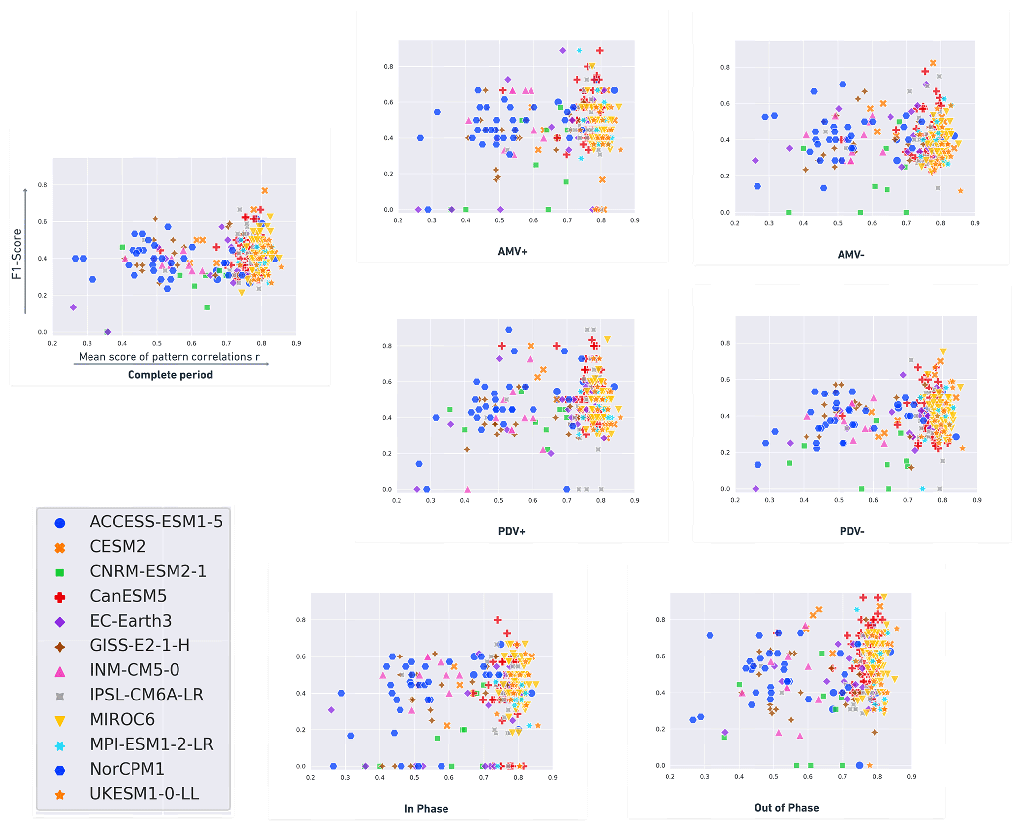
Figure 10 Scatter plots: R_coef mean score (spatial correlation with reanalysis – x axis) vs. F₁ score (network similarity with respect to reanalysis – y-axis) during the different regimes. Spatial correlation values do not change from one regime to another; these are the same mean scores calculated from the Pearson r coefficients of the four modes in Sect. 3.1 over the 1900–2014 period. Similarly to Fig. 9, scatter plots are shown only for the long regimes.

In Fig. 10, we plot the F₁ scores for all realizations (color- and marker-coded by CMIP6 ensemble; see the legend) for the long regimes with respect to the mean score of r spatial correlations from Sect. 3.1. Similarly to Fig. 9, we choose not to show the scatter plots for the short regimes. As the mean scores of spatial correlations are the same for all regimes (computed between the regression maps for the whole 1900–2014 time series of the indices), how high (low) a single scatter point can get during a certain regime reveals its causal network similarity (dissimilarity) to reanalysis during that regime. The scatter points closer to the top right corner of each plot belong to realizations which better simulate the spatial patterns and causal fingerprints of reanalysis. Considering only the complete-period panel (upper left in Fig. 10), the upper right corner of this panel mainly shows realizations from CESM2 (orange crosses), MIROC6 (yellow triangles) and CanESM5 (red plus signs) models. From the same panel, we can notice, for example, that the UKESM1-0-LL realizations (orange five-pointed stars) have great spatial pattern similarity with reanalysis. These UKESM1-0-LL realizations, however, do not show high similarity when comparing their causal fingerprint to that concluded from reanalysis data. The same can be said about MPI-ESM1-2-LR realizations (cyan six-pointed stars) which, in spite of their high level of skill in recreating the spatial regression patterns of the four modes of climate variability, fail to obtain F₁ scores as high as those from CESM2, CanESM5 or MIROC6 during most regimes. It is only during the AMV+ and out-of-phase regimes that very few MPI-ESM1-2-LR simulations exceed the 0.7 F₁ score bar. Overall, we can conclude that CESM2 (orange crosses), CanESM5 (red plus signs) and MIROC6 (yellow triangles) undoubtedly outperform other LEs in this evaluation. This is proven through the consistency that simulations from these three LEs show in resembling the observed causal fingerprints during the different regimes. Despite obtaining high spatial correlation coefficients, two members of the IPSL-CM6A-LR model (gray scatters) show the best network similarity with reanalysis during the PDV+ regime, while three other members of this model show no similarity during the same regime.

It is worth mentioning that the number of realizations within an LE appears to increase the chance of a model comprising a simulation with similar dependency structures as those found in observations. The three simulations with the highest F₁ scores during the out-of-phase regime (see Fig. 8) belong to either CanESM5 or MIROC6, which are the LEs with the highest number of realizations (65 and 50 ensemble members, respectively). This is likely related to the number of realizations needed to capture similar random internal variability to that observed in reanalysis data. This is less valid for the CESM2 model, which, with only 11 realizations, contains simulations with high F₁ scores during most of the regimes shown in Fig. 10. In general, modeling centers previously contributed only a small number of realizations to international climate change projection assessments [e.g., phase 5 of the CMIP (CMIP5; Taylor et al., 2012)]. As a result, model-associated errors and internal climate variability remained difficult, if not impossible, to disentangle (Kay et al., 2015). In this paper, as CMIP6 includes LE models, we overcome this sampling problem by using at least 10 realizations per model (see Table 1). In this way, we have a better estimate of the natural internal variability and the externally forced part. The larger the ensemble size, the more likely it is that the observed internal variability falls within the plausible internal-variability range simulated by those particular LE model realizations. However, despite the improvement of CMIP6 models in capturing the different modes of climate variability (Fasullo et al., 2020), recent studies already pointed to persisting tropical Atlantic biases that knew little or no improvement compared to CMIP5 (Richter and Tokinaga, 2020; Farneti et al., 2022). These biases certainly affect the simulation of Atlantic variability within CMIP6 models, as they project additional uncertainties onto the AMV−related causal dynamics and spatial patterns. Moreover, previous research showed that, on the decadal timescale, Atlantic mean SST biases in CMIP5 models are directly related to the variability of trade winds over the region (Kajtar et al., 2018). McGregor et al. (2018) found that the addition of the CMIP5 Atlantic bias leads to enhanced descending motion trends in the western and eastern Pacific and a reduced trend in the central Pacific. The same study found that the observed northward migration of the Intertropical Convergence Zone (ITCZ) is absent when introducing CMIP5 Atlantic bias.

The spatial pattern correlation analysis (Fig. 4), the resulting F₁ scores with respect to reanalysis (Fig. 8a) and the CMIP6 pairwise network comparisons (Fig. 9) call for the investigation of the coupling attributes and the simulated internal variability in the CNRM-ESM2-1 ensemble, as its realizations clearly fail to reproduce the observed spatial patterns and causal links between modes of climate variability compared to other CMIP6 LEs. The relatively large distribution of spatial correlation values for the simulated PNA and PDV modes (see purple and red boxes of CNRM-ESM2-1 in Fig. 4b) suggests spatial disagreement between the realizations of the CNRM-ESM2-1 model with regards to the expressed PNA and PDV patterns. This might be the result of a relatively large distribution of forced PNA and/or PDV trends. This can be supported by the time series metrics provided by CVDP-LE, which reveal that, among the models analyzed in this paper (see Table 1), CNRM-ESM2-1 holds the largest 10th–90th percentile range of linear PDV trends (−0.89 per 115 years to 1.18 per 115 years) during the 1900–2014 period. These values can be found on the PDV time series ensemble summary figure (https://webext.cgd.ucar.edu/Multi-Case/CVDP-LE_repository/CMIP6_Historical_1900-2014/pdv_timeseries_mon.summary.png, last access: 17 March 2023) as part of the historical 1900–2014 CMIP6 variability diagnostic results distributed by the CVDP-LE authors (Phillips et al., 2020). Considering the fact that the model only counts 10 realizations, the large 10th–90th percentile range reveals that the forced PDV trend can be significantly different from one CNRM-ESM2-1 simulation to another. This not only translates to the dissimilarity in terms of spatial PDV patterns within the ensemble members but most probably leads to very different causal dynamics too. The latter can be seen through the causal networks in Figs. A1 and A2 in the Appendix, where CNRM-ESM2-1 simulations hardly agree on the sign of the PDV–PNA links (appearing with lighter shades of red) compared to the other CMIP6 models (where PDV–PNA links appear with darker shades of red).

In the present work, we defined regimes explicitly based on the phases of PDV and AMV. There are also methods to agnostically extract underlying regimes and their corresponding causal graphs from time series (Saggioro et al., 2020), but these are not reliable for the small sample sizes in combination with the high dimensionality of the present datasets.

4 Summary

Applying PCMCI+ to reanalysis data revealed that the direct decadal opposite-sign response from AMV to PDV, described by Meehl et al. (2021a), occurs not only during the analysis of the complete 1900–2014 period (with 11-year time lag) but also during several specified regimes: PDV− (11-year lag), AMV− (11-year lag), PDV+/AMV− (1- and 11-year lags) and when PDV and AMV are out of phase (1- and 11-year lags). These regimes vary from being 34-years long (for PDV+/AMV−) to being 65-years long (for out-of-phase). For the shorter PDV+/AMV+ regime (25-years long), we detect a positive same-sign response from AMV to PDV with a 4-year time delay. The causal networks constructed from the reanalysis datasets have also revealed the same-sign response from PDV to AMV during the following two regimes: PDV− (59-years long) and PDV−/AMV+ (31-years long). In other words, the regime-oriented causal analysis indicates that AMV might serve as an early predictor of decadal variability over the Pacific. We also find an indirect connection between the Atlantic and Pacific, which is established via PNA during AMV− and PDV+ regimes (both 59-years long) and during PDV−/AMV+. The latter is one of the two regimes that feature a same-sign response from PDV to AMV. An indirect connection between the Atlantic and the Pacific via the Pacific–South American pattern is found during the complete 1900–2014 period, where AMV is positively linked with PSA1 but PSA1 has a negative lagged link to PDV. During the AMV− regime, the causal graph shows opposite-sign AMV → PSA1 → PDV lagged connections.

As an example for the regime-oriented causal analysis of CMIP6 models, we showed the CanESM5 ensemble-averaged causal graphs, which indicate that the opposite-sign effect of AMV on PDV (blue AMV → PDV link) is recreated by several realizations (38 out of 65) during the out-of-phase regime, agreeing with the reanalysis results and the literature findings (Newman et al., 2016; Johnson et al., 2020). In the Appendix, Figs. A1 and A2 show that this opposite-sign lagged effect of AMV on PDV was clearly present in simulations belonging to CESM2 and MIROC6 ensembles (AMV → PDV links are clearly blue). The PDV teleconnection to PNA in the form of mutual same-sign response (positive cross-MCI links) was clearly present not only in most realizations of the CanESM5 model (Fig. 7) but also in most of the CMIP6 LE simulations analyzed. This is true considering the exception of the CNRM-ESM2-1 simulations, which show less agreement with each other regarding the sign of the PDV–PNA links (appearing with lighter shades of red in Figs. A1 and A2) compared to the other CMIP6 models.

The evaluation of the large ensembles from the CMIP6 archive presented in this paper unveiled how a model performs compared to other models in terms of simulating observed spatial patterns and causal pathways between modes of climate variability. Most CMIP6 models were found to score better during the out-of-phase regime, with CESM2, CanESM5, MIROC6 and MPI-ESM1-2-LR being the best performers during this regime. We showed the importance of using LEs in causal model evaluation to address the sampling issue, and we explained the possible causal pathways during specific regimes that might not appear in causal networks constructed from reanalysis data. Several CanESM5 realizations suggested a same-sign AMV → PDV link during the in-phase regime. This link did not appear on the in-phase-regime causal graph reconstructed from reanalysis. This same-sign response is nonetheless documented by previous research (Wu et al., 2011; Meehl et al., 2021a). The CanESM5 and MIROC6 models with the highest number of members were found to outperform other models in simulating observed causal patterns during the long regimes (see Fig. 8a). Interestingly, the CESM2 model, with a relatively smaller ensemble size (11 realizations), was also found to display larger causal fingerprint similarity with reanalysis during the long regimes. The causal network similarity between different CMIP6 LE models was also assessed throughout this paper. Simulations from CESM2, CanESM5 and MIROC6 models also largely resemble each other and those from the MPI-ESM1-2-LR model in terms of estimated causal networks during most regimes (Fig. 9).

A deepened intra-model comparison remains essential to evaluate how realizations of the same model ensemble differ from one another. The “ripf” identifier of every simulation within the CMIP6 LEs used in this study shows that some LEs only include realizations (r) with the same initialization (i), physics (p) and forcing (f), while other LEs contain realizations with different physics or forcing. On that account, it is of high importance that the documentation provided by modeling groups be inspected regarding the relevant realization attributes of their model ensemble.

Causal model evaluation also helps to better understand remote contributions to internal variability over specific regions. As we are not subtracting the ensemble mean (representing the forced response), the causal links found when analyzing observational reanalysis and CMIP6 historical simulations are thus expected to include external-forcing contributions, especially those from space- and time-varying aerosol radiative forcing. It is therefore crucial to separate the internal-variability component from the externally forced part to gain a better understanding on the effects of external forcings on Atlantic–Pacific interactions. Meehl et al. (2021a) recently examined this effect through time series pacemaker experiments in which the effects from aerosols are removed (by fixing aerosols at 1920 values). The approach and findings presented here motivate a follow-up study where pacemaker, pre-industrial control and future scenario simulations are to be analyzed through causal discovery algorithms to reveal the impact of climate change on the teleconnections and interactions between major modes of climate variability. Overall, the regime-oriented causal model evaluation followed in this study has the potential to be a powerful methodology that can be applied in a number of environment-related topics, offering tremendous insight to improve the understanding of the complex Earth system and the state of the art of climate modeling.

Appendix A

Table A1 Distribution of Pearson r correlation values between the simulated (CMIP6 LE) and observed (ERA20C_ERA5, ERSSTv5) spatial patterns of PNA, PSA1, PDV and AMV and their mean scores over the 1900–2014 period. Sorted in alphabetical order.

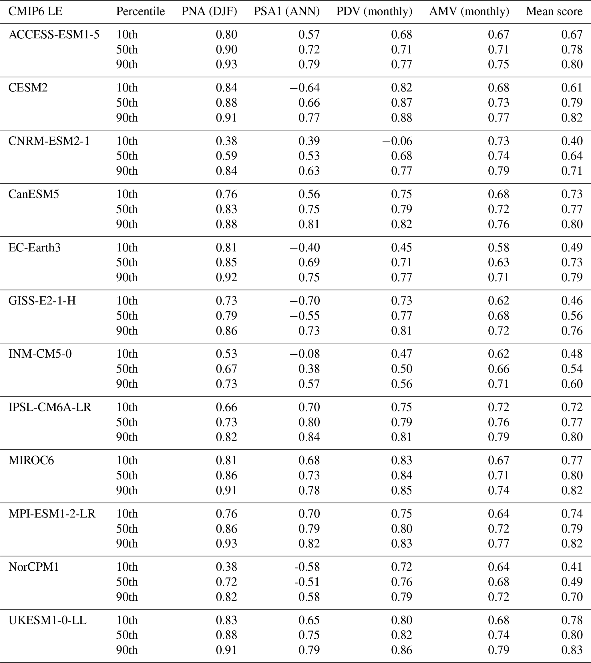
Table A2 Pearson correlation values obtained using 18 UKESM1-0-LL simulation with respect to the observed (ERA20C_ERA5, ERSSTv5) spatial patterns of PNA, PSA1, PDV and AMV and their mean score over the 1900–2014 period. Sorted by mean score.

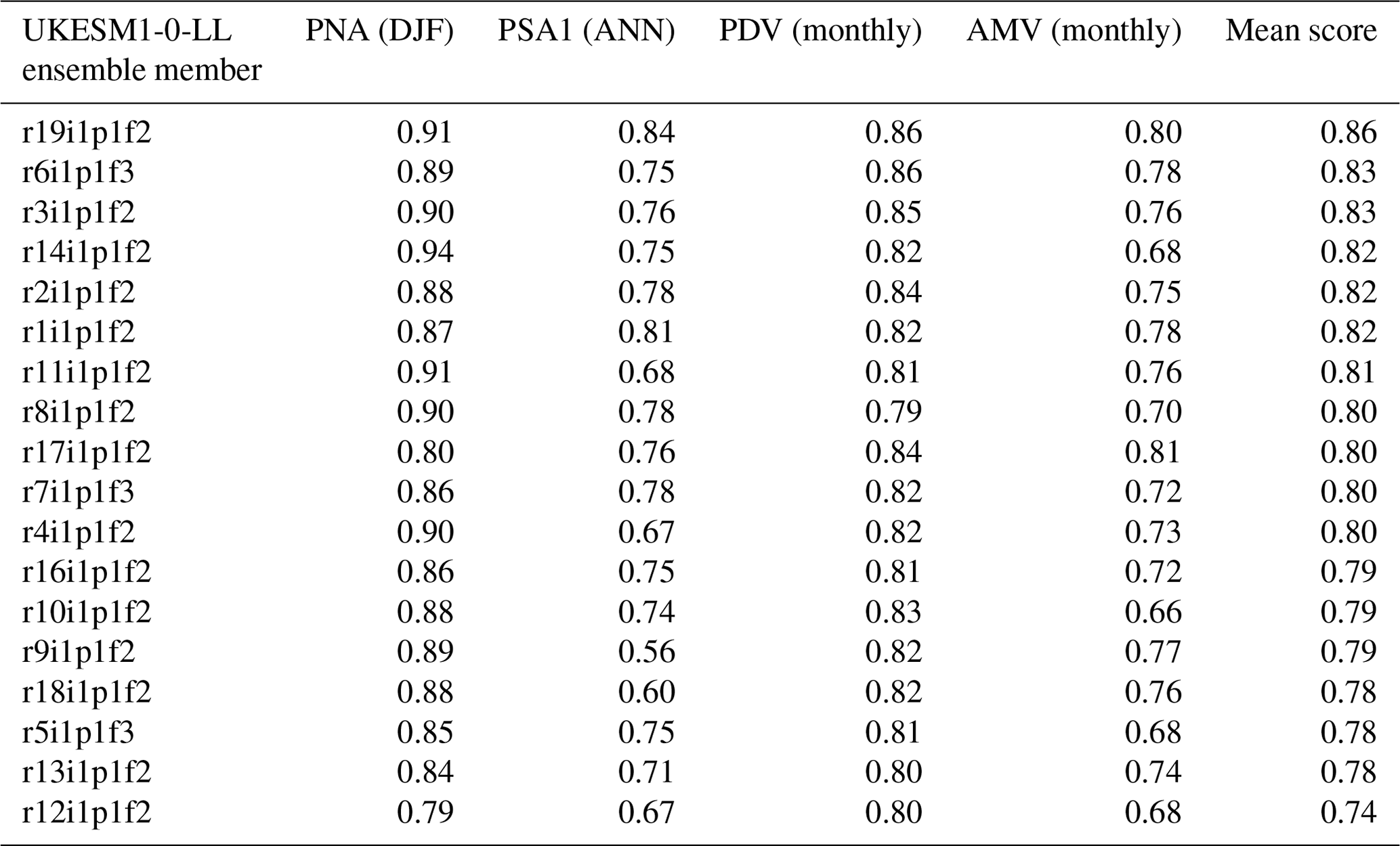
Table A3 Cross-MCI and auto-MCI values calculated by PCMCI+ from reanalysis time series data for the complete 1900–2014 period. Values are relative to the complete-period causal graph shown in Fig. 2 (right panel) and in Fig. 5 (upper left panel). The table presents the cross-MCI (cross-correlation) values denoting the sign and strength of the causal link between node i and node j for lags between 0 and τ_max. In bold are the highest absolute cross-MCI values for that specific link (detected within the statistical significance threshold, α_pc≤0.05) and for which links are apparent on the causal graphs. The values are rounded to 2 decimal places.

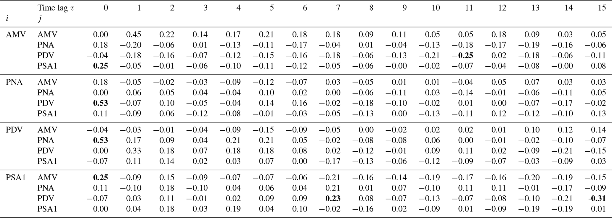
Table A4 Number of years for every regime for reanalysis and CMIP6 simulations 1–40.

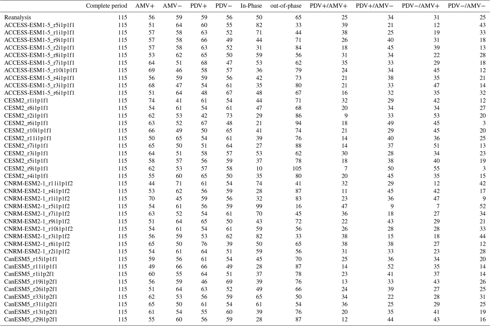
Table A5 Number of years for every regime for reanalysis and CMIP6 simulations 41–80.

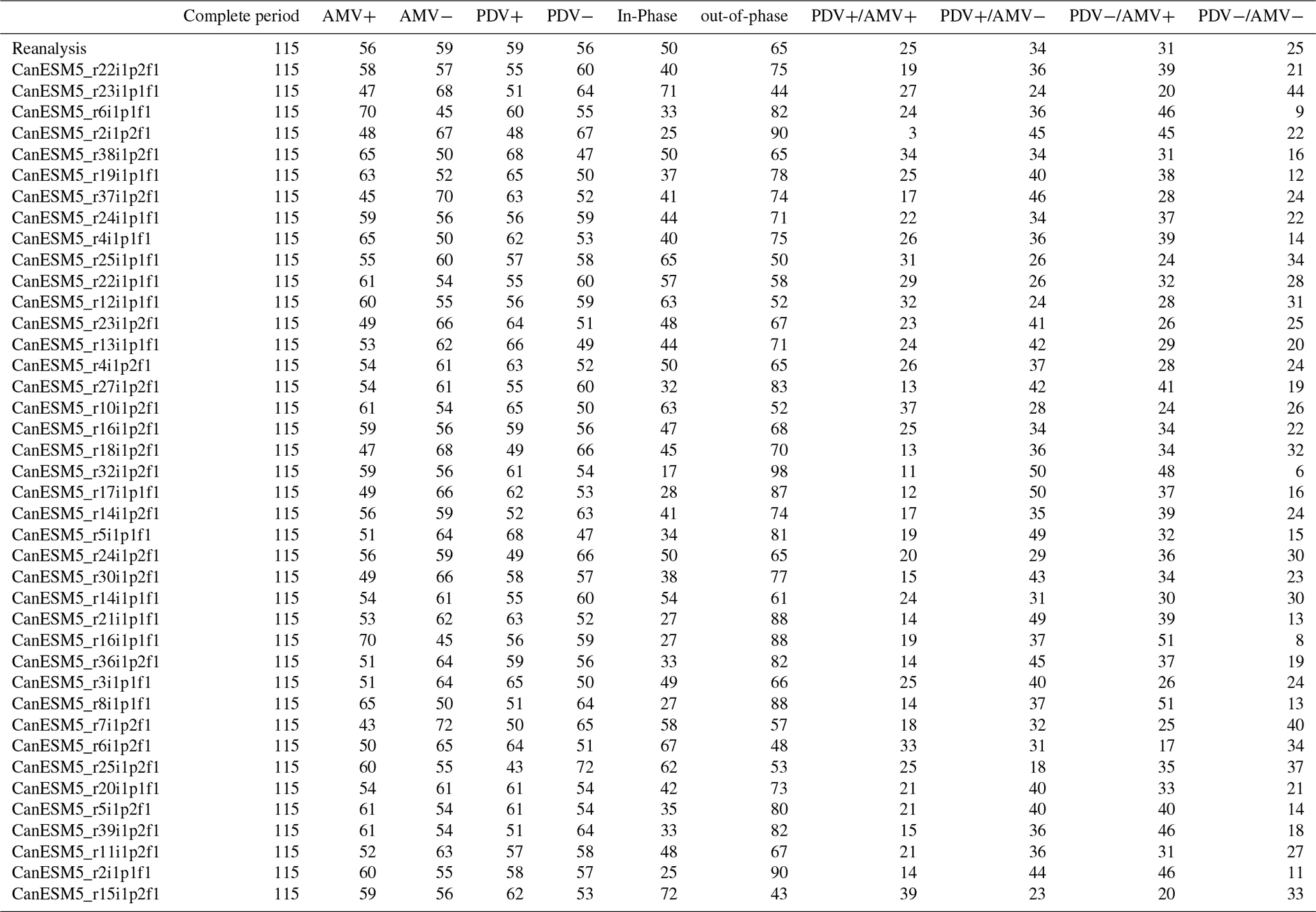
Table A6 Number of years for every regime for reanalysis and CMIP6 simulations 81–120.

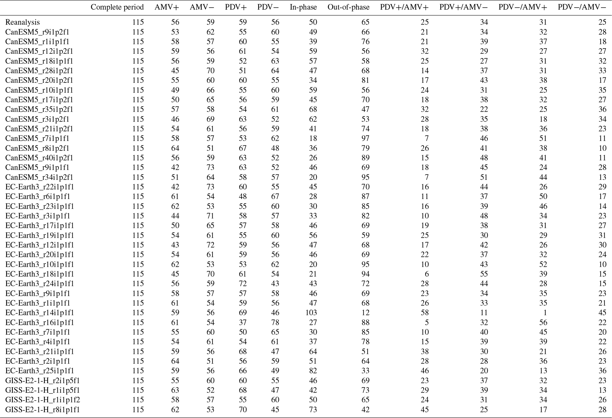
Table A7 Number of years for every regime for reanalysis and CMIP6 simulations 121–160.

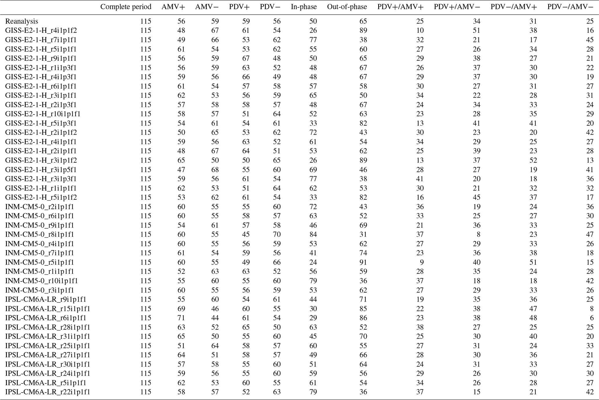
Table A8 Number of years for every regime for reanalysis and CMIP6 simulations 161–200.

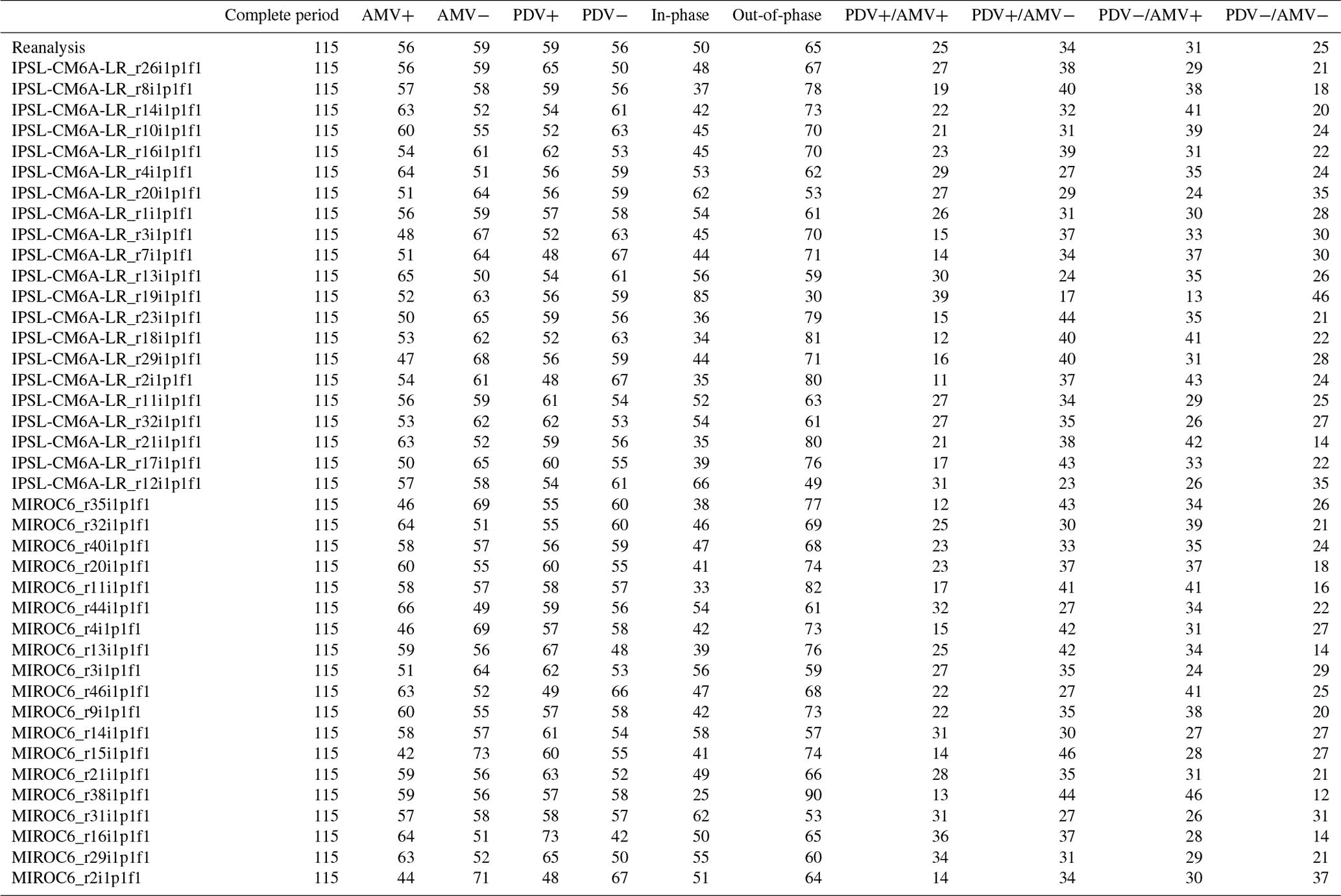
Table A9 Number of years for every regime for reanalysis and CMIP6 simulations 201–240.

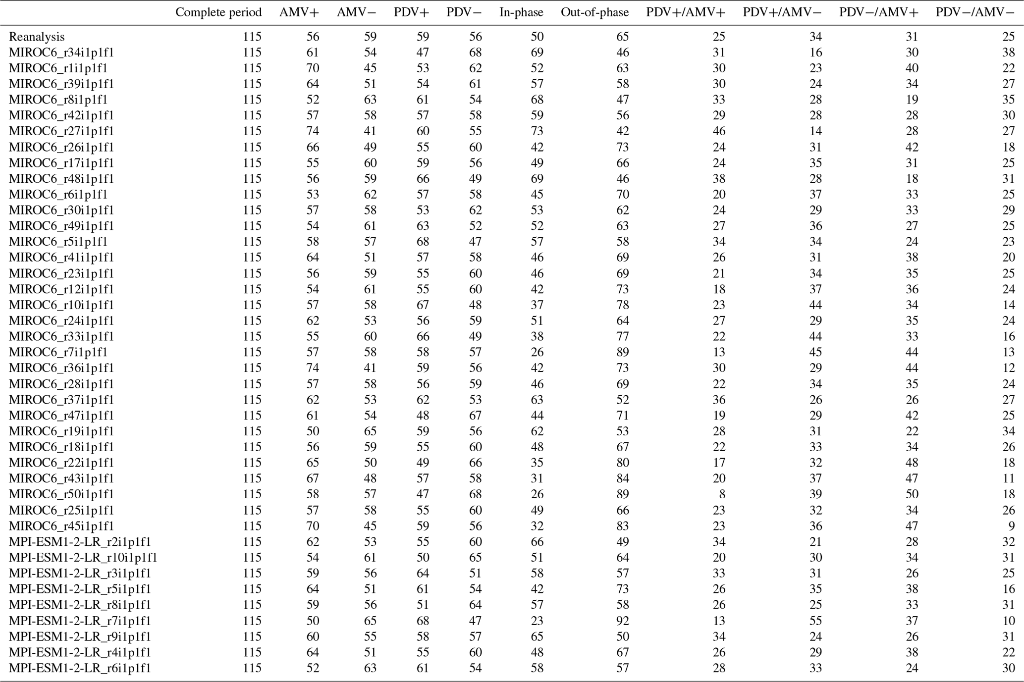
Table A10 Number of years for every regime for reanalysis and CMIP6 simulations 241–289.

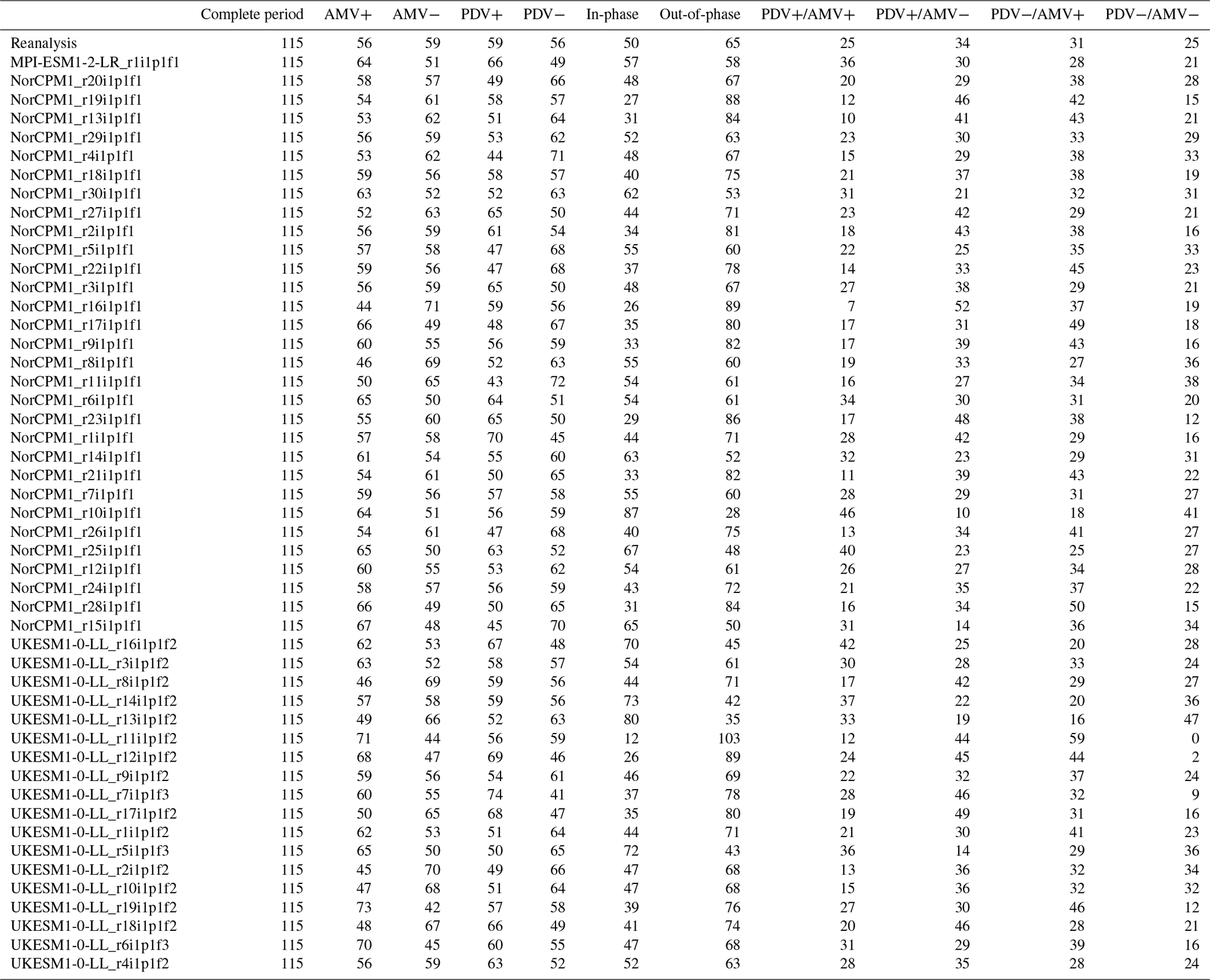
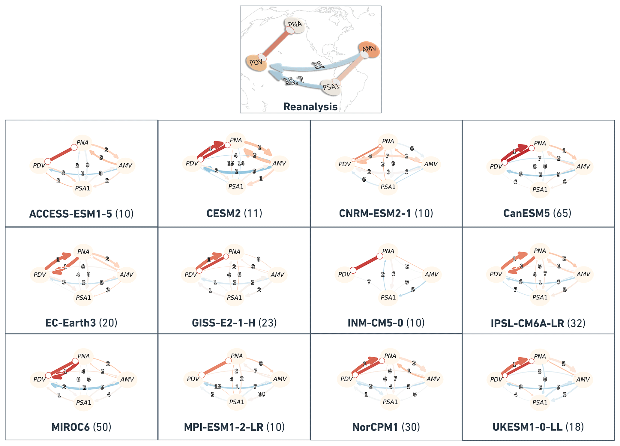
Figure A1 Similar to Fig. 7 but for the 12 CMIP6 models during the complete 1900–2014 period. Each panel has a label stating the model name and the number of ensemble members between parentheses. The auto-MCI values were not taken into consideration.

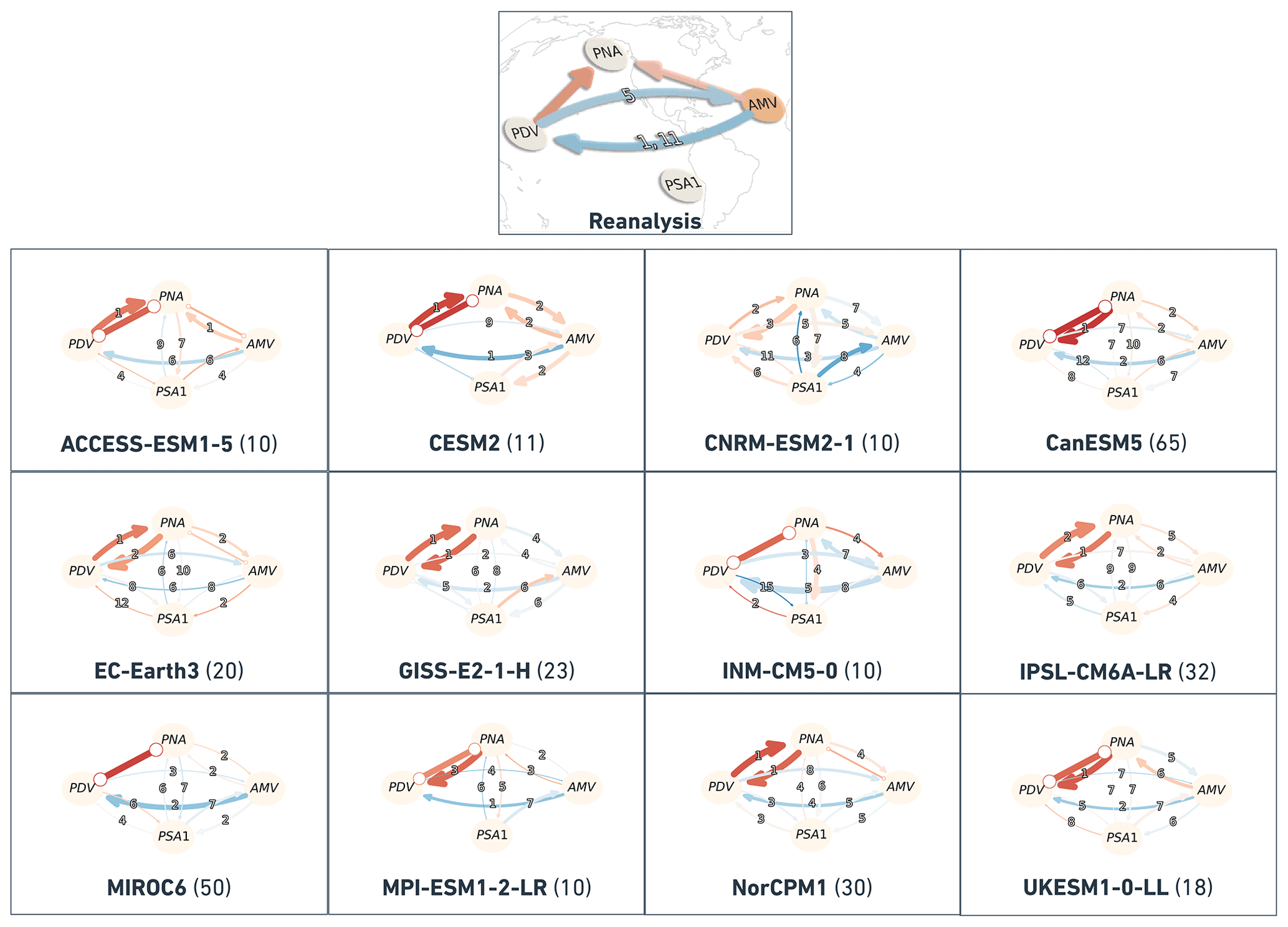
Figure A2 Similar to Fig. 7 but for the 12 CMIP6 models during the out-of-phase regime. Each panel has a label stating the model name and the number of ensemble members between parentheses. The auto-MCI values were not taken into consideration.

Figure A3 Similar to Fig. 7 but for the 12 CMIP6 models during the in-phase regime. Each panel has a label stating the model name and the number of ensemble members between parentheses. The auto-MCI values were not taken into consideration.