the Creative Commons Attribution 4.0 License.
the Creative Commons Attribution 4.0 License.
 | 04 Jul 2022
Effect of the Atlantic Meridional Overturning Circulation on atmospheric pCO2 variations
Anna S. von der Heydt
Henk A. Dijkstra
Proxy records show large variability of atmospheric pCO2 on different timescales. Most often such variations are attributed to a forced response of the carbon cycle to changes in external conditions. Here, we address the problem of internally generated variations in pCO2 due to pure carbon cycle dynamics. We focus on the effect of the strength of Atlantic Meridional Overturning Circulation (AMOC) on such internal variability. Using the Simple Carbon Project Model v1.0 (SCP-M), which we have extended to represent a suite of nonlinear carbon cycle feedbacks, we efficiently explore the multi-dimensional parameter space to address the AMOC–pCO2 relationship. We find that climatic boundary conditions and the representation of biological production in the model are most important for this relationship. When climate sensitivity in our model is increased, we find intrinsic oscillations due to Hopf bifurcations with multi-millennial periods. The mechanism behind these oscillations is clarified and related to the coupling of atmospheric pCO2 and the alkalinity cycle, via the river influx and the sediment outflux. This mechanism is thought to be relevant for explaining atmospheric pCO2 variability during glacial cycles.
- Article
(3369 KB) - Full-text XML
- BibTeX
- EndNote


Atmospheric pCO2 values show large variations on many different timescales. Over the Cenozoic, pCO2 values gradually decreased from values of up to 2500 ppmv in the Eocene to 300 ppmv at the end of the Pliocene. When considering the Pleistocene glacial–interglacial cycles, one of the remarkable results is the strong correlation between pCO2 and temperature, with dominant variations of about 100 ppmv in 100 000 years, as reconstructed from ice cores (Petit et al., 1999). Over the industrial period, pCO2 values have increased by 130 ppmv due to human activities (Friedlingstein et al., 2020). This forced trend is superposed on natural variability associated with the seasonal cycle and longer-timescale climate variability (Gruber et al., 2019). The effect of the natural variability is much lower than the forced trend on such relatively short timescales. For example, the El Niño–Southern Oscillation (ENSO), a dominant mode of interannual climate variability, induces atmospheric pCO2 variations of only 1–2 ppmv (Jiang and Yung, 2019). Most studies seek to explain such variations in pCO2 as a forced response of the carbon cycle to changes in external conditions. For example, glacial cycles are thought to be caused by orbital variations in insolation, possibly amplified by physical processes in the climate system (Muller and MacDonald, 2000). Such variations in temperature (and other quantities, e.g., precipitation) then affect the carbon cycle, leading to changes in pCO2. On the other hand, changes in pCO2 will affect global mean temperature and hence may amplify any temperature anomaly. Hence it is questionable whether the pCO2 response to orbital insolation changes can be considered as a solely forced response, with no internal dynamics of the carbon being involved (Rothman, 2015).
The carbon cycle is comprised of an extremely complex entangled set of processes which act in the different components of the climate system (e.g., land, ocean) on many different timescales. The marine carbon cycle, with its three main carbon pumps, is a major player in this cycle, at present day resulting in the uptake of about 25 % of human-released emissions (Sabine et al., 2004). The carbon pumps involve physical processes, biological processes, and processes in ocean sediments. Many carbon cycle feedbacks exist, either between only physical quantities or between biological and physical quantities. An example of such a feedback is the solubility feedback: for higher atmospheric pCO2, solubility of CO2 decreases due to higher ocean temperatures, resulting in relatively less CO2 uptake by the ocean and thus relatively higher atmospheric pCO2. Given this strongly nonlinear system, it would be strange if it would not show strong internal variability, i.e., variability which would exist even if the carbon cycle system were driven by a time-independent external forcing. There are indeed examples (Rothman, 2019), where oscillatory behavior in the carbon cycle has been attributed to internal carbon cycle dynamics.
The physical context of all carbon pumps is the three-dimensional ocean circulation, which can be roughly decomposed in a wind-driven and an overturning component, the latter strongly related to the deep-ocean circulation. The Atlantic Meridional Overturning Circulation (AMOC) is a major component of the global overturning circulation because of its associated meridional transport of heat, salt, and nutrients.
The relation between the AMOC and atmospheric pCO2 is complicated. A direct effect of a changing AMOC is a change in the distribution of tracers such as temperature, dissolved inorganic carbon (DIC), alkalinity (Alk), and nutrients. For example, after an AMOC weakening, the distributions of these tracers affect biological export production via reduced nutrient upwelling (Marchal et al., 1998; Menviel et al., 2008; Mariotti et al., 2012; Nielsen et al., 2019) and gas exchange via changing solubility of CO2 in the ocean (Menviel et al., 2014). Besides these direct effects, the AMOC also influences mixing in the Southern Ocean. Changes in this mixing due to a weaker AMOC can result in a higher outgoing flux of carbon to the atmosphere (e.g., Schmittner et al., 2007; Huiskamp and Meissner, 2012; Menviel et al., 2014). Furthermore, changes in the AMOC also influence the general sensitivity of the marine carbon cycle to, for example, changes in the wind field (Munday et al., 2014). These processes form a complex puzzle where the sign of atmospheric pCO2 change following an AMOC strength change is difficult to determine. Currently, different models produce different results with respect to the sign of the atmospheric pCO2 change, which can be attributed to the assessed timescale, model used, and what climatic boundary conditions are used (Gottschalk et al., 2019).
On the other hand, pCO2 also influences the AMOC (Toggweiler and Russell, 2008), and present-day climate models forced with anthropogenic emissions simulate a weaker AMOC for larger atmospheric pCO2 (Gregory et al., 2005; Weijer et al., 2020). By contrast, proxy data suggest that in the Last Glacial Maximum both atmospheric pCO2 and the strength of the AMOC were lower (Duplessy et al., 1988). This shows that there is also a sensitivity to climatic boundary conditions in the relation (Zhu et al., 2015) between the AMOC and atmospheric pCO2. The AMOC can also display tipping behavior (Weijer et al., 2019) under an increase in pCO2, which can have large effects on climate. Examples of these effects are disrupted heat transport (Ganachaud and Wunsch, 2000), changing precipitation patterns (Vellinga and Wood, 2002), and a different distribution of important tracers in the ocean. Such tipping can hence have strong consequences on the carbon cycle, and hence on atmospheric pCO2.
In this paper, we perform a systematic study of internal carbon cycle variability and the relation AMOC–pCO2 connection, using the Simple Carbon Project Model v1.0 (SCP-M). This model (O'Neill et al., 2019) simulates the most important carbon cycle processes in a simple global ocean box structure. The simple box setup enables us to efficiently scan the parameter space of the carbon cycle model using parameter continuation methods. With this approach we aim to answer the following three questions: (i) how does atmospheric pCO2 respond to changes in the strength of a constant (in time) AMOC? (ii) Does the pCO2–AMOC feedback lead to new variability phenomena? And (iii) are there tipping points and internal oscillations in the carbon cycle?
When answering these questions, we pay special attention to different (non-linear) carbon cycle feedbacks. We will also use two different model configurations to take account of different climatic boundary conditions, the pre-industrial (PI) configuration and the Last Glacial Maximum (LGM) configuration. The SCP-M, its configurations, the different additional feedbacks implemented, and the parameter continuation approach are described in Sect. 2. In Sect. 3 we present the results of the different cases considered, and we conclude the paper with a summary and discussion in Sect. 4.
2.1 SCP-M
The SCP-M is a carbon cycle box model focused on the marine carbon cycle. Because of its simple structure, it is well suited to test high-level concepts in both modern and past configurations. In the ocean several tracers are resolved. In this study we will only use the three most important tracers, DIC, Alk, and phosphate (), to reduce the problem size. In the original model there is also a terrestrial biosphere component, and several sources of CO2 to the atmosphere. We will not use these, since our focus is on the marine carbon cycle. The processes which are resolved are ocean overturning circulation, sea–air gas exchange, biological production, calcium carbonate (CaCO3) production and dissolution, and river and sediment fluxes.
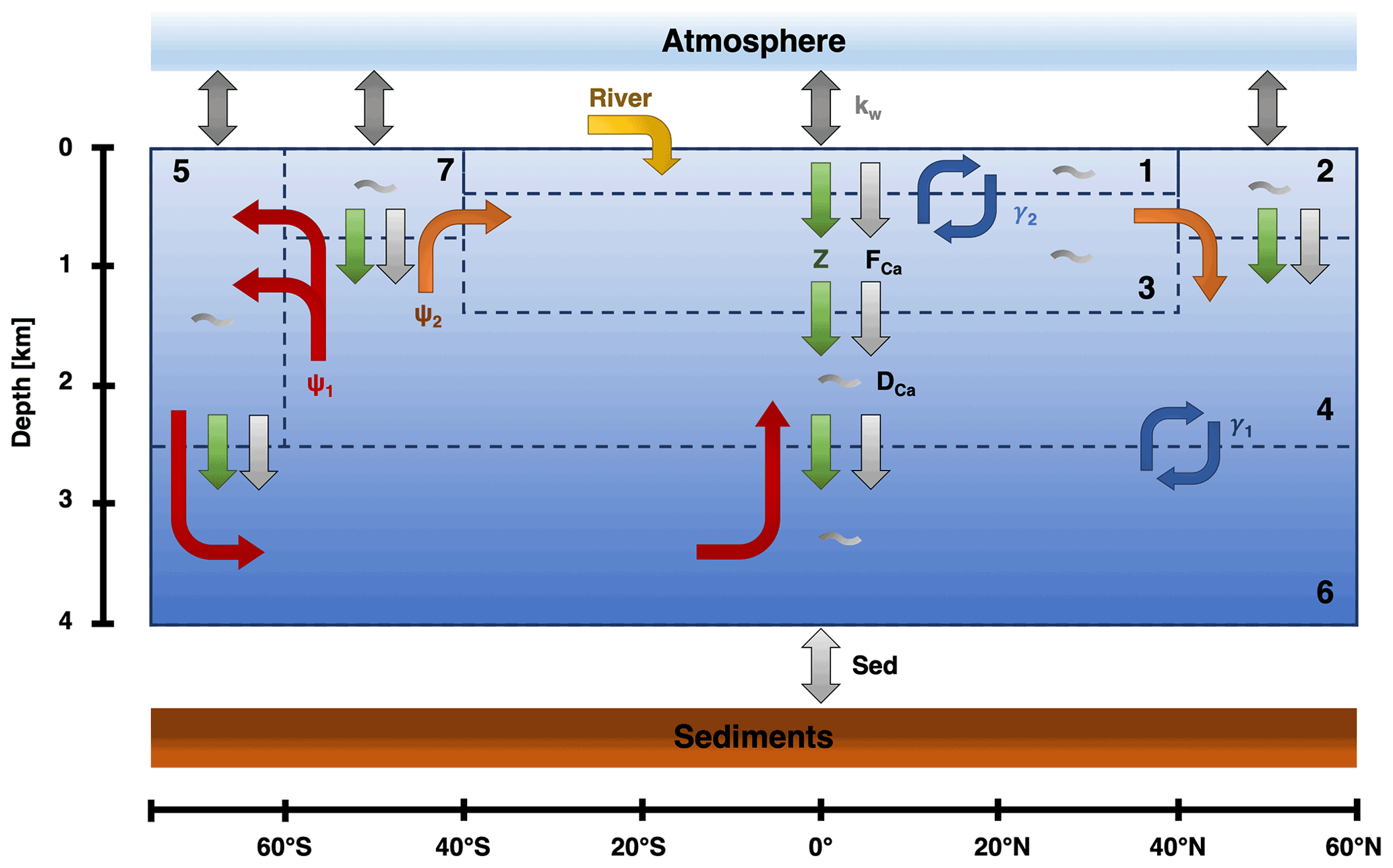
Figure 1The box structure and fluxes for the SCP-M based on O'Neill et al. (2019). ψ1 (red) is the GOC, ψ2 (orange) is the AMOC, and γ1 and γ2 (blue) represent bidirectional mixing. Biological fluxes are represented by the green arrows, calcifier fluxes by the light gray arrows, and general dissolution of calcium carbonate by the gray wiggles in the boxes. kw (gray) represents the gas exchange between the ocean and the atmosphere. Lastly, there is an influx in box 1 via the rivers (yellow) and an outflux to the sediments (light gray).
The model consists of eight boxes: one atmospheric box and seven oceanic boxes (Fig. 1). This means that the sediment stock is not explicitly solved for in the model. In the model, the ocean boxes are differentiated on latitude and depth. Consequently, there is no longitudinal variation, and no differentiation between ocean basins. The used boxes are (1) a low-latitude surface box, (2) a northern high-latitude surface box, (3) an intermediate ocean box, (4) a deep-ocean box, (5) a southern high-latitude surface box, (6) an abyssal ocean box, and (7) a sub-polar surface box. This division in the ocean is based on regions in the ocean where the water masses have similar characteristics. The different boxes are connected via ocean circulation and mixing, which is based upon a conceptual view of the ocean circulation (Talley, 2013). The largest circulation is the Global Overturning Circulation (GOC; ψ1). This circulation connects boxes 4–7 and represents the formation of Antarctic Bottom Water. Next to the GOC, the other major circulation is the AMOC (ψ2) which connects boxes 2–4 and 7. Lastly, there is bidirectional (vertical) mixing between boxes 4 and 6 (γ1) and boxes 1 and 3 (γ2).
To be able to solve for several fluxes, such as the air–sea gas exchange, the pH in the ocean needs to be determined. Unfortunately, pH is not a conservative tracer, which means that we need a carbonate chemistry module to solve for pH. In the SCP-M, a direct solver is used where the pH value of the previous time step is used as an estimate for the new step (Follows et al., 2006). Using this carbonate chemistry, the model is able to determine the carbonate () concentration and oceanic pCO2. This latter quantity is used to model the exchange of CO2 between the atmosphere and ocean. For each surface box, the flux is proportional to the pCO2 difference between atmosphere and ocean and a constant piston velocity (kw).
Biological production is constant in the SCP-M. Per surface box, a constant value is used to denote the biological export production at 100 m depth. The organic flux is remineralized in the subsurface boxes following the power law of Martin et al. (1987). The biological export production is also important for the carbonate pump. Via a constant rain ratio, the biological production is linked to the production of calcifiers. Besides organic growth via photosynthesis, calcifiers also take up DIC and Alk to form shells (CaCO3). Upon death, these calcifiers sink to deeper boxes where the shells are dissolved. The dissolution of the shells is dependent on a constant dissolution rate and a saturation-dependent dissolution. If the total dissolution of CaCO3 in the ocean is smaller (larger) than the production in the surface ocean, there is an outflux (influx) of DIC and Alk to (from) the sediments. The river flux for is constant in the SCP-M and balanced by a constant outflux into the sediments. Influx of DIC and Alk via the rivers is variable and proportional to atmospheric pCO2 according to
where WSC is a parameter reflecting constant silicate weathering, WSV a parameter representing variable silicate weathering, WCV a parameter representing variable carbonate weathering, and pCO2atm the partial pressure of CO2 in the atmosphere. This relation was already used in the SCP-M and is directly taken from Toggweiler and Russell (2008), meaning no adaptations were made to the relation or to the parameter values. This expression is adapted from a formulation used in Walker and Kasting (1992). The two different processes parameterized here, carbonate and silicate weathering, are important on different timescales. Terrestrial carbonate weathering is typically important on timescales of 103 to 104 years, whereas silicate weathering balances volcanic carbon input on timescales of 105 to 106 years (Archer et al., 1997).
The difference between the influx of DIC and Alk and the outflux into the sediments determines the change in total carbon and Alk in the system. The outflux of DIC and Alk via the sediments i, is related to CaCO3 burial, which is the difference between CaCO3 production in the surface ocean and CaCO3 dissolution in the ocean and sediments. CaCO3 dissolution consists of two parts: a saturation-driven part and a constant part following
where the first part is related to the saturation state: . If the saturation state is larger than 1, the saturation-dependent dissolution is zero, and only the constant term remains (DC). CaCO3 production is linearly dependent on biological production using a rain ratio.
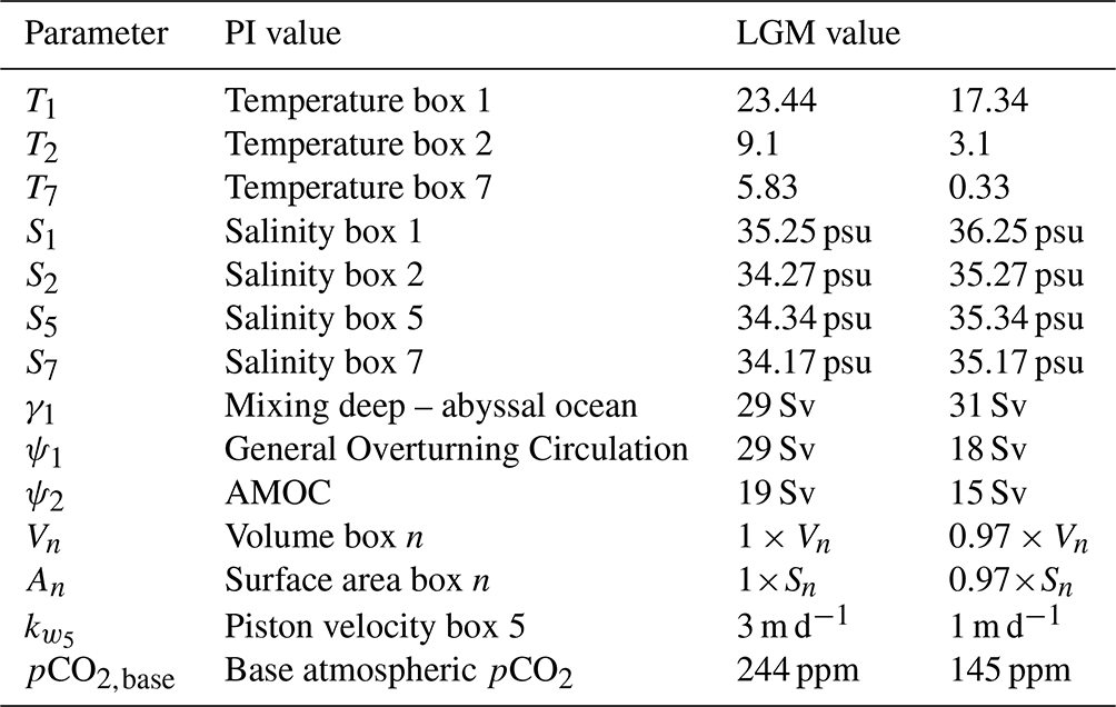
A big advantage of the SCP-M is that it has two configurations: a PI configuration and an LGM configuration. The parameter values in both configurations have been determined via extensive tuning of the model to observations and proxies in O'Neill et al. (2019). The configurations are differentiated on surface ocean temperature and salinity, ocean circulation, sea ice cover in box 5, and total volume of the ocean. The parameter values of the two different SCP-M configurations can be found in Table 1.
Table 1The parameter values that are different between the two configurations (PI and LGM). In columns 1 and 2 the parameter symbol and description are given. In column 3 the PI value is given, and in column 4 the LGM value is given.
2.2 Representation of carbon cycle processes and feedbacks
The carbon cycle has many (non-linear) feedbacks which are not represented in the original SCP-M version to keep the model as simple as possible. The absence of these feedbacks can lead to non-physical behavior (e.g., negative concentrations) when parameter values, such as the AMOC strength, are changed. We have implemented several additional feedbacks which can be divided into two categories: those that mostly concern physical processes and those associated with biological processes. The feedbacks are included through parameters λ; when such a parameter is zero, the feedback is not active in the SCP-M and the original version applies. For all feedbacks, except the feedback on the rain ratio (Eq. 11 below), the sign of the feedback (positive or negative) is unclear beforehand as multiple (carbon cycle) processes are involved.
2.2.1 Physical processes
An important feedback is the coupling of temperature to atmospheric pCO2. There are several ways temperature effects the carbon cycle. For example, decreasing temperatures increase the solubility of CO2, which results in more uptake of CO2 by the ocean. For this feedback, we make a distinction between box 5 and boxes 1, 2, and 7. Box 5, the southern high-latitude surface box, is more isolated than the other boxes due to the Antarctic Circumpolar Circulation (ACC). Therefore, we have included the option in the model to use a different sensitivity in box 5. The temperature in the boxes is calculated as follows.
Here Ti,base is the base temperature in the SCP-M. The change in temperature is dependent on atmospheric pCO2 and a base value of atmospheric pCO2. This base value is the steady-state solution in the SCP-M without feedbacks (Table 1). Climate sensitivity can be changed via the λ parameters. For a λ of 1, sea surface temperatures increase 2 K per CO2 doubling. As a reference, a 2 K warming for surface air temperatures is at the lower end of the range found in CMIP6 models (Zelinka et al., 2020).
Besides an effect on solubility, temperature can also affect the piston velocity. In the often used (Wanninkhof, 1992) formulation, the piston velocity is dependent on temperature via the Schmidt number (Eqs. 6 and 7). In our model, we use this dependency on the Schmidt number, which causes the piston velocity to increase for warmer temperatures. Hence
where
In these equations, kw is the used piston velocity, kw,base is the piston velocity in the SCP-M (3 m d−1), and T is the temperature of the box in degrees Celsius. The λ parameter needs to be either 0 (constant piston velocity, as in SCP-M) or 1 (variable piston velocity). Notice that if the temperature feedback is used (λT>0), the Schmidt number depends on atmospheric pCO2.
2.2.2 Biological processes
A large limitation in the original SCP-M is the constant biological production. Nutrient availability introduces a large constraint on biological production, but this process is completely absent in the original SCP-M. This process is introduced in the model here by adopting the expression used in the Long-term Ocean-atmosphere-Sediment Carbon cycle Reservoir model (LOSCAR) (Zeebe, 2012). In LOSCAR, production is dependent on the upwelling of nutrients, which in our model translates to the following expressions.
In these equations Z represents the production in the surface box, and Zbase the value used in the original SCP-M. Furthermore, α is the fraction of ψ1 that moves from box 4 to box 7, and ϵ is the biological efficiency in the box. As with the piston velocity, λBI is either 0 (SCP-M) or 1. Notice that the current branch represented by ψ1, which flows from box 4 to box 5, does not influence the production in box 5. We do not use this branch, since it is assumed to flow into box 5 below the euphotic zone.
In Eq. (8a–d) the biological efficiency (ϵ) is also introduced. There are studies (e.g., Cael et al., 2017) where they relate biological efficiency to temperature. We have adopted a simple linear relation to represent the influence of temperature on biological efficiency, i.e.,
In this equation, λϵ controls how strong the relation is between the efficiency and temperature change (ΔT). In addition, ϵbase is the base value of the biological efficiency. These values have been fitted so that Z is equal to Zbase under the original parameter values in the SCP-M.
In the SCP-M, is the only nutrient. In the real ocean, additional nutrients play a role in biological production, one of them being nitrate (). During photosynthesis, organisms take up nitrate, and thereby increase Alk. This biological influence on Alk is not incorporated in the SCP-M but is present in many other models (e.g., Kwon and Primeau, 2008). We have included this influence as follows:
In this equation ABio is the biological flux affecting Alk. This flux is related to the DIC biological flux (CBio) and the N:C Redfield ratio (). For this relation, the λBA parameter can be 0 (not included, original SCP-M) or 1 (included).
Finally, we have also included a feedback for the rain ratio, which is the fraction of calcifiers in the total biological production. In the original SCP-M this is a constant value for all boxes. Calcifiers can be limited in growth when concentrations are too low. Ridgwell et al. (2007) model this limitation via the saturation state of CaCO3 as
Here, FCa is the used rain ratio, and FCa,base is the value used in the original SCP-M (0.07). The saturation state is determined via the concentrations of calcium ([Ca]), the carbonate ion concentration [], and an equilibrium constant Ksp. In this feedback, λF is either 0 (SCP-M) or 1. The rain ratio feedback is a negative feedback. When carbonate concentrations increase in the surface layer, the rain ratio increases, and therefore more calcium carbonate is removed from the surface layer, effectively lowering the carbonate concentration.
2.3 Parameter continuation methodology
The SCP-M, including our representations of the additional feedbacks, leads to a system of ordinary differential equations of the form
where u is the state vector (containing all the dependent quantities in all boxes), f contains the right-hand side of the equations, and p is the parameter vector. Usually, such models are integrated in time from a certain initial condition, and the equilibrium behavior is determined for different values of the parameters. However, this is not very efficient to scan the parameter space, and, moreover, it is difficult to detect tipping behavior. A much more efficient approach is to determine the equilibrium solutions directly versus parameters, avoiding time integration, using continuation methods.
Here, we use the continuation and bifurcation software program AUTO to scan the parameter space and detect bifurcations efficiently (Doedel et al., 2007). The SCP-M is very suitable to be implemented into AUTO and to easily compute branches of equilibrium solutions, such as steady states of Eq. (12), versus parameters. The equations of the SCP-M turn out to have a singular Jacobian matrix (because carbon, alkalinity, and phosphate quantities are determined up to an additive constant), which requires adding integral conservation equations. We have added such integral conservation equations for carbon (DIC and atmospheric pCO2), Alk, and to the model equations to replace the equations for box 4. The conservation law for is straightforward and already present in the model equations. The constant influx of via the rivers is equal to the constant outflux via the sediments.
In the original SCP-M model, carbon and Alk are conserved in the ocean, atmosphere, continents, and sediments. However, the continental and sediment stocks are not explicitly represented in the version of the SCP-M we use. However, we can describe the change of total carbon and total Alk in the combined atmosphere and ocean stocks over time as
In these equations “TC” and “TAlk” are the total carbon and alkalinity in the system. As with , total carbon and Alk change due to influx via the rivers (Criver and Ariver) and outflux via the sediments. The carbon outflux via the sediments is determined by the sum of carbonate (Ccarb) and biological (Cbio) fluxes in the system. For Alk, the biological influence is absent. Model simulations with the original SCP-M have shown that the influence of the biological fluxes is negligible; i.e., all biologically produced organic matter is respired in the ocean itself. Therefore, this term can be set to zero in Eq. (13a). This makes Eq. (13b) proportional to Eq. (13a), and hence we include only the latter and use it to determine the change in total Alk in the model.
We also changed the carbonate chemistry in the model. The original SCP-M uses the algorithm of Follows et al. (2006), which solves the carbonate chemistry by using hydrogen ion concentrations from a previous time step. Therefore, the algorithm is inherently transient and, since we directly solve for steady-state solutions, not suitable. We therefore adopted a simple “textbook” carbonate chemistry based on carbonate alkalinity (Williams and Follows, 2011; Munhoven, 2013). This method approximates oceanic pCO2 by assuming that Alk is equal to carbonate alkalinity (). A disadvantage of this method is that pH values are generally a bit higher (0.15–0.2) than using more complicated algorithms (Munhoven, 2013). These higher pH values are one of the reasons our atmospheric pCO2 values are lower than in the original SCP-M (approximately 60 ppm for case P-CTL described in Sect. 3).
Eventually, by including Eq. (13a) and the overall conservation equations, the version of SCP-M used is a dynamical system with a state vector of dimension d=20. There is one equation for atmospheric pCO2; there are six for DIC, Alk, and in the ocean; and there is one equation for the total carbon content. Except for the new carbonate chemistry, the necessary changes made to the SCP-M do not change the outcome of the model compared to the original model. When the original model is fitted with the same carbonate chemistry based on carbonate alkalinity, the AUTO implementation and the original code produce the same results.
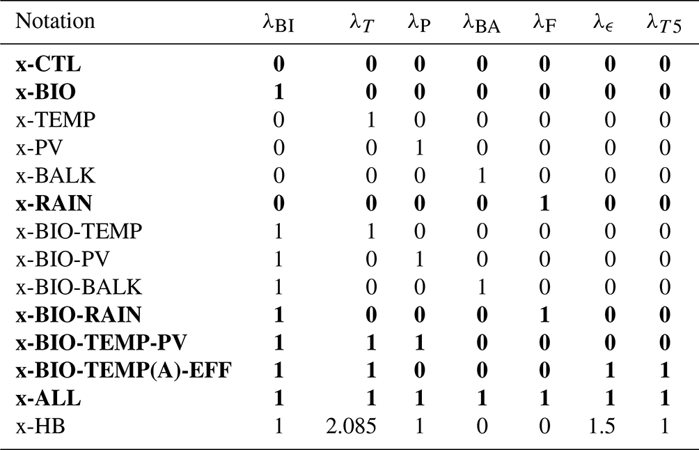
In Sect. 3.1 we present the general sensitivity of atmospheric pCO2 to variations in the AMOC strength. We extend these results in Sect. 3.2 by adding a coupling between the AMOC strength and atmospheric pCO2. Internal variability found in the model will be presented in Sect. 3.3. An overview of all cases considered is given in Table 2. Our control experiment uses the original model, which is tuned to accurately represent the pre-industrial and last glacial maximum carbon cycle. From this “realistic” model we investigate the sensitivity of the carbon cycle to specific carbon cycle feedbacks that can be found in more detailed models. By gradually increasing the number of feedbacks in the model, we can assess the effects of the (combined) feedbacks.
Table 2Overview of the cases considered and their notation. The left column displays the used feedback. The other columns show the notation and what feedbacks are included in the specific case. The “x” in the notation is replaced with either P for the PI configuration or L for the LGM configuration. Bold rows indicate that this combination of feedbacks is also used for cases with a coupling between the AMOC and atmospheric pCO2 (Sect. 3.2). For these cases, “C” is added to either “P” or “L=” to denote the coupling. The last column represents the feedback combinations used in Sect. 3.3. Case x-CTL is the original SCP-M.
3.1 Sensitivity of atmospheric pCO2 to the AMOC
In this section the AMOC strength is used as a control parameter, and steady states are calculated versus this parameter. For each configuration (PI and LGM) we use three reference cases (x-CTL, the original SCP-M configuration; x-BIO, with a different parameterization for biological production; and x-ALL, with all feedbacks included, in Table 2, where x is either P for the PI or L for the LGM configuration). The steady-state value of atmospheric pCO2 versus AMOC is shown for the reference cases in Fig. 2, where all branches represent stable fixed points. For the cases where the biological feedback is not included, the solutions for smaller values of AMOC ( Sv) display negative concentrations in box 2 and hence are not allowed. Such boundaries can be automatically monitored in AUTO, and the continuation is stopped once a boundary is exceeded.
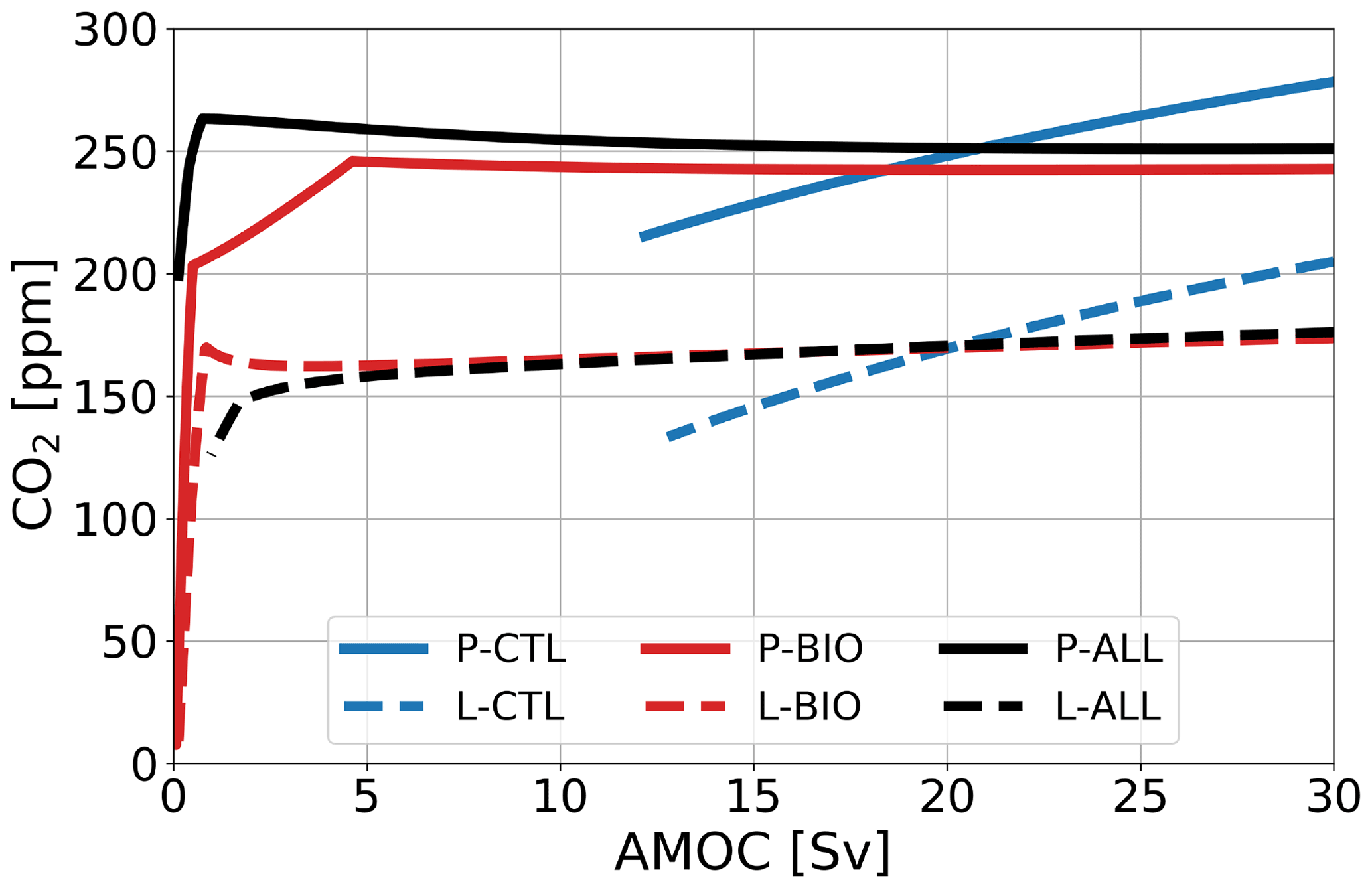
Figure 2Atmospheric pCO2 in parts per million under varying AMOC strength in sverdrups for three reference cases (blue: no feedback; red: with biological feedback; black: all feedbacks) in two configurations (solid: PI; dashed: LGM). All branches represent stable fixed points.
For the PI configuration, Fig. 2 shows that, whereas pCO2 increases for larger AMOC strengths in the P-CTL case, it remains fairly constant in P-BIO and P-ALL. Atmospheric pCO2 in the P-BIO case peaks around 5 Sv and then decreases until approximately 20 Sv, after which it increases slightly again. This different behavior occurs because, in the P-BIO case, the AMOC has competing influences on DIC concentrations of the surface ocean. A first effect of an increasing AMOC is to increase the ventilation of the deep ocean, which also increases DIC concentrations in the surface layer. This promotes outgassing to the atmosphere. However, by increasing the AMOC strength, biological production in boxes 2 and 7 is also increased. As a result, DIC and are transported from the surface layer to the deep ocean. The first effect is dominant after 20 Sv and the second effect in the range of 5 to 20 Sv. The absence of the second effect in P-CTL explains the difference in sensitivity between P-CTL and P-BIO. P-ALL behaves fairly similarly to P-BIO, except in the regime with a weak AMOC strength ( Sv). This behavior is caused by the saturation-dependent rain ratio.
When we look at the other cases (Fig. 3a), we see that they either behave qualitatively like P-CTL (the cases without “BIO”) or behave like P-BIO (cases with “BIO”). Looking in more detail, we can see that when we include the rain ratio feedback (cases P-RAIN, P-BIO-RAIN) atmospheric pCO2 is higher, and when we include the biological influence on alkalinity, atmospheric pCO2 is lower (cases P-BALK, P-BIO-BALK). The results in Fig. 3a show that the biological feedback (λBI=1) is the most dominant feedback in the PI configuration; i.e., including this feedback leads to a completely different sensitivity of the carbon cycle to changes in the AMOC strength.
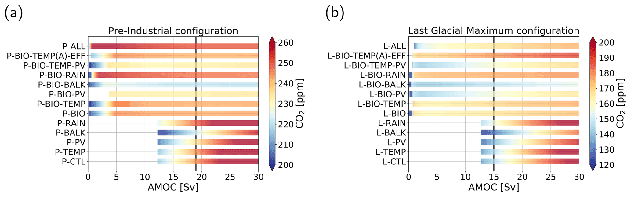
Figure 3Atmospheric pCO2 in parts per million (color shading) under varying AMOC strength in sverdrups for the cases considered in Table 2. (a) Pre-industrial configuration. (b) Last Glacial Maximum configuration. Note that the range of the color shading differs between the two configurations and that some CO2 concentrations fall outside the displayed range. The AMOC ranges of the bars differ, because for some cases the steady solution becomes nonphysical (e.g., negative concentrations or large subzero temperature). The vertical black lines represent the AMOC strength in the original SCP-M.
For the LGM configuration (Fig. 2), two important differences with respect to the PI configuration appear: (1) atmospheric pCO2 is approximately 80 ppm lower, and (2) the L-BIO and L-ALL cases have a different sensitivity than the P-BIO and P-ALL cases for lower AMOC values. Where in P-BIO atmospheric pCO2 decreases for an increasing AMOC between 5 and 20 Sv, L-BIO shows a monotonous increase in atmospheric pCO2 from 3 Sv onward. We see this different relation because in the LGM configuration, deep-ocean ventilation, which can be seen as the sum of the GOC and AMOC, is lower due to a weaker GOC. Consequently, deep-ocean ventilation is more sensitive to changes in the AMOC. This eventually causes the different response of the L-BIO and L-ALL cases with respect to the P-BIO and P-ALL cases. The L-TEMP to L-BIO-TEMP(A)-EFF cases (Fig. 3b) relate to the L-CTL and L-BIO cases as in the PI configuration. Figure 3b shows that in the LGM configuration, as is the case in the PI configuration, the biological feedback is most dominant. The other feedbacks only influence the offset of CO2 concentrations, but they do not result in large changes to the relation between the AMOC and atmospheric pCO2.
3.2 Coupling AMOC–carbon cycle
The AMOC strength also depends on atmospheric pCO2, and below we will discuss the steady-state model solutions when a coupling between the AMOC and atmospheric pCO2 is applied. This coupling is based on how the AMOC responds to increasing atmospheric pCO2 in CMIP6 models (e.g., Bakker et al., 2016) and given by
In this equation ψ2,base is a base value of the AMOC taken from the uncoupled case (where the AMOC is prescribed), ψ2 is the actual AMOC strength in m3 s−1 in the coupled case, and λA determines the strength of the coupling. We use three different values of λA in this section: (1) 0 (no coupling), 1 (20 % decrease for a CO2 doubling), and 4 (80 % decrease for a CO2 doubling). As the AMOC strength ψ2 is now part of the state vector, we need other quantities as control parameters. We will use three different parameters here: (1) the rain ratio (FCa), (2) the biological production (Z), and (3) the piston velocity (kw). We have chosen these three parameters since they (approximately) represent the three carbon pumps: the carbonate pump, the soft tissue pump, and the solubility pump We follow the steady-state solution in these parameters, where possible, between 0.1 and 10 times the reference value (indicated by the multiplier in Fig. 4). This large, though not necessarily realistic, range is used to test the sensitivity of the carbon cycle to the parameters, and to see whether bifurcations can arise in the carbon cycle.
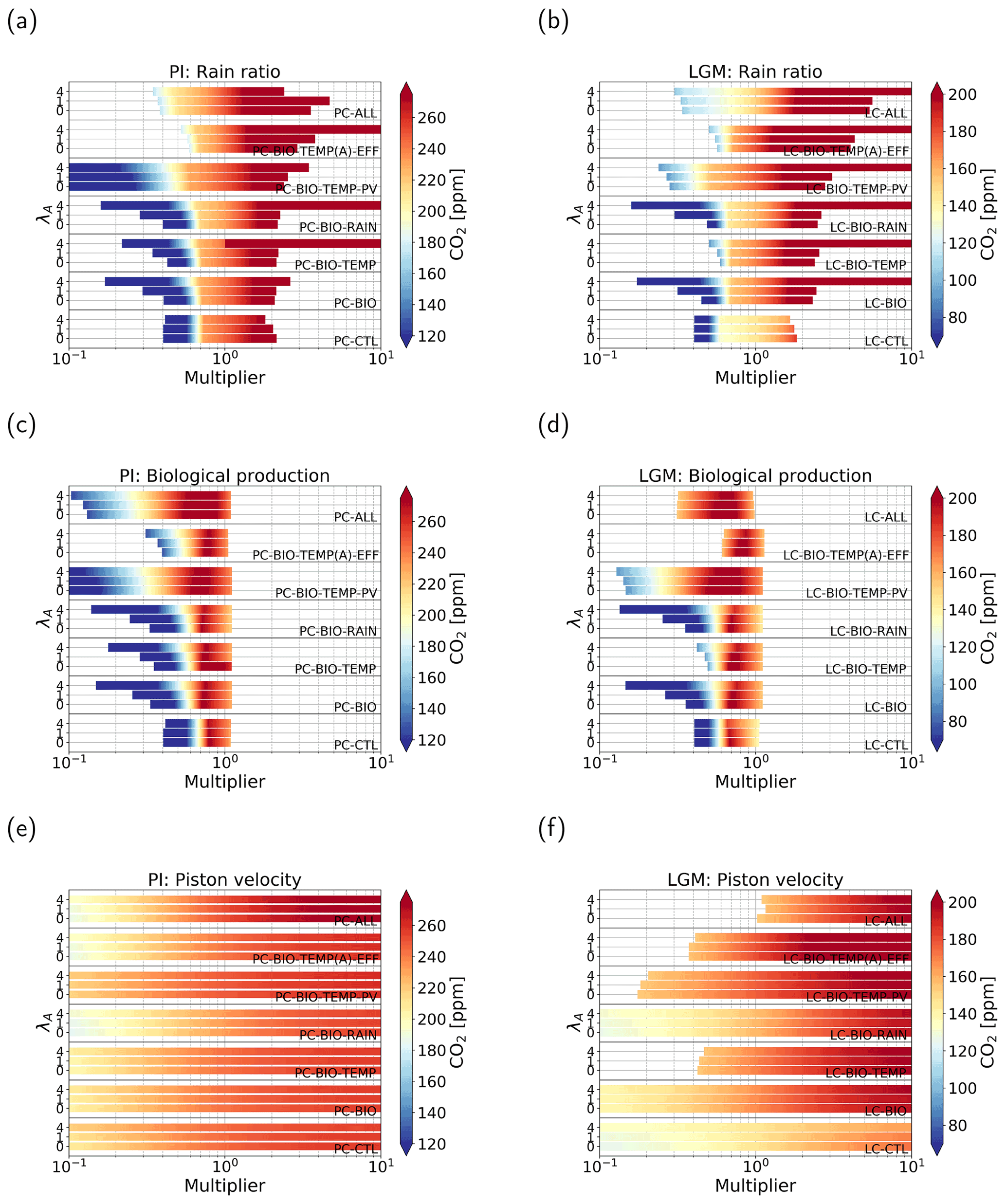
Figure 4Atmospheric pCO2 in parts per million (color shading) under varying parameter values. Panels (a, c, e) represent cases of the PI configuration and (b, d, f) of the LGM configuration. Panels (a, b) show cases where the strength of the rain ratio is varied between 0.1 and 10 times the original value. Panels (c)–(f) show the same but for cases where biological production (c, d) and the piston velocity (e, f) are varied. In total seven feedback combinations are used, denoted by the text within the graph. For each case, three different coupling strengths have been used: (1) λA=0, (2) λA=1, and (3) λA=4.
When we look at the effect of increasing λA, i.e., the coupling, we see that the general sensitivity of the solution to changes in model parameters decreases. This effect is best seen in the LC-CTL case, but also present in the other cases, though less pronounced.
In Fig. 4a and b we plot the results when we use the rain ratio as a control parameter in the continuation. There are no large differences between the different cases and configurations. Generally, we see two regimes. For low rain ratios, the solution is quite sensitive to changes in the rain ratio. Where the coloring in Fig. 4a and b is yellow (around 230 ppm for the PI and around 140 ppm for the LGM configuration), we see a shift: the solution becomes less sensitive to changes in the rain ratio. To explain the regimes of sensitivity, we note that the CaCO3 production is linearly related to the rain ratio. The production minus the dissolution of CaCO3 in the water column determines the outflux of Alk and DIC via the sediments. The different regimes can be explained by the amount of CaCO3 dissolution in the deep and abyssal ocean. For low rain ratios, the saturation state in the ocean is larger than 1, which means there is no saturation-driven dissolution and only constant dissolution. This makes the outflux of Alk and DIC linearly proportional to the production: if the rain ratio is low, the outflux is also low. Because we are looking at a steady-state solution, this decrease in burial has to be compensated for by a weaker influx, i.e., a lower river influx. This is only possible when atmospheric pCO2 is lower. For larger rain ratios, we have both saturation-dependent and constant dissolution in the subsurface boxes, i.e., more dissolution in the water column. Due to the variable dissolution, the outflux of Alk and DIC is no longer fully determined by CaCO3 production. This results in a lower sensitivity of the outflux to changes in the rain ratio. Therefore, atmospheric pCO2 is also less sensitive to the rain ratio.
For biological production as a control parameter (Fig. 4c and d) again all cases show comparable behavior. We can see that the parameter range for higher biological production is short. This is because concentrations become negative at this point, even when we include the biological feedback. All cases have a maximum in atmospheric pCO2 around 0.7–0.8 times the original value. When the multiplier is lower than this value, we see a positive relation (higher biological production, higher atmospheric pCO2). For values larger than the maximum, we see an opposite relation, i.e., lower atmospheric pCO2 for higher biological production. This second regime is generally what we would expect when biological production is increased; i.e., when biological production removes more carbon from the surface layer, more carbon can be taken out of the atmosphere by the surface ocean, which reduces atmospheric pCO2. The first regime is not what we would expect at first, but this can be explained by the same mechanism as for the rain ratio: reduced biological production leads to low production of CaCO3, leading to low burial rates of CaCO3. Lower burial rates lead to lower river influx because the sources and sinks of alkalinity to the ocean balance, which can only be achieved by decreasing atmospheric pCO2. Again, increasing the AMOC coupling only reduces the sensitivity of the solutions.

Figure 5(a) Bifurcation diagram for case L-HB in atmospheric pCO2–AMOC space. Blue solid lines denote stable steady states (or fixed points, FPs), red dashed lines indicate unstable steady states, black solid lines indicate a stable limit cycle (LC), and the black square denotes the location of a (supercritical) Hopf bifurcation (HB). (b) The oscillation of atmospheric pCO2 in parts per million versus time in years for the limit cycle at 15 Sv. The period is 5814 years.
In Fig. 4e and f, we plot the results when we use the piston velocity parameter (kw) as a control parameter. By the gradually changing colors, we can see a logarithmic relation with higher sensitivities for lower piston velocities. The different feedbacks, configurations, and coupling strengths have the same effect as for the other two control parameters discussed above.
3.3 Internal oscillation
The feedback strengths we have used so far have been quite modest. The continuation methodology enables us to efficiently look at cases with different feedback strengths and to see whether different combinations can induce bifurcations in the carbon cycle, and by extensively scanning the parameter space we found such bifurcations. Especially in the LGM configuration, when climate sensitivity (λT) and the biological efficiency feedback (λϵ) are increased, bifurcations arise on the branches of steady solutions. With case L-HB (for parameter values, see Table 2), we present an example where we find a supercritical Hopf bifurcation (HB) around 13 Sv (Fig. 5a) in the uncoupled case (λA=0, so the AMOC strength is a control parameter again). The HB produces a stable limit cycle extending to larger AMOC strengths with a period between 5000 and 6000 years where all state variables oscillate. In this section we look at the internal oscillation at 15 Sv (Fig. 5b). The oscillation has a period of 5814 years, and atmospheric pCO2 has a range of 72 ppm.
The HB described in this section exists for a large range of parameter values and is thus robust. One important constraint on the existence of the bifurcation is the coupling strength between atmospheric pCO2 and biological production. This coupling comes down to the effect of atmospheric pCO2 on the biological efficiency (ϵ), which can be increased by increasing the temperature feedback (λT) and/or the efficiency feedback (λϵ). We do not find this bifurcation in the PI configuration, because when the biology feedback (λBI=1) is included, atmospheric pCO2 is insensitive to changes in the AMOC strength (P-BIO case, Fig. 2). Because of this low sensitivity, surface ocean temperature and biological efficiency are also insensitive to changes in the AMOC strength in the PI configuration. Therefore, the coupling between the two is less effective in this configuration, and we do not find a HB.
To explain the mechanism behind the oscillation, we have to look at the time-dependent solution of the model. What is important for this oscillation is the coupling between atmospheric pCO2 and the alkalinity cycle. Alkalinity influences the gas exchange between the ocean and the atmosphere via the carbonate chemistry and is, in turn, influenced by atmospheric pCO2 because the source and sink of alkalinity are coupled to pCO2. The source, the river influx, is directly proportional to atmospheric pCO2 according to Eq. (1).
The sink, i.e., outfluxing via the sediments, is related to CaCO3 burial, which is the difference between CaCO3 production in the surface ocean and CaCO3 dissolution in the ocean and sediments (Eq. 2). In the oscillation, the saturation state of CaCO3 in the ocean is larger than 1 everywhere. This happens when the river influx is larger than the biogenic flux in the surface ocean (Zeebe and Westbroek, 2003), which is plausible for the past oceans. Therefore, total dissolution in the ocean is constant and does not vary. This means that CaCO3 burial becomes a function of CaCO3 formation and thus of biological production. Since this production is dependent on the biological efficiency, which is directly proportionate to atmospheric pCO2, the sink is also influenced by atmospheric pCO2. However, the effect of atmospheric pCO2 on the source and sink is opposite. When atmospheric pCO2 is high, the river influx is high, while the sediment outflux is low. This is key to the general mechanism sketched in Fig. 6.

Figure 6Schematic representation of the mechanism of the internal oscillation. The rectangles represent state variables, while the pointed blocks represent fluxes or model parameters. Some boxes have thicker outlining. These boxes cause a chain of events. The chains corresponding to the box are the boxes with the same color shading. The gray and blue rectangles in the background represent a quarter period. In the second half of the period, processes are replaced with a dashed line. These processes are the opposite of what happens in the first half of the period.
The results show that atmospheric pCO2 is affected by the amount of ingassing into box 1. Therefore, we start the explanation of the oscillation in Fig. 6 at this point. At the beginning of the oscillation (time t=0 in Fig. 6), ingassing in box 1 starts to decrease. As a result, atmospheric pCO2 starts to increase approximately 200 years later. There is a delay, since atmospheric pCO2 is not solely determined by the gas exchange with box 1. The increase in atmospheric pCO2 has multiple effects. First of all, temperatures start to increase, which lowers biological efficiency. This in turn reduces CaCO3 production, and thus the sink of alkalinity is also reduced. Another effect of increasing atmospheric pCO2 is an increasing river flux, i.e., an increasing source of alkalinity into the ocean. After a quarter period (time in Fig. 6), the source becomes larger than the sink, and total alkalinity in the ocean starts to increase. Meanwhile, atmospheric pCO2 is still increasing. As a result, the river influx also keeps increasing, while the sediment outflux keeps decreasing. After half a period (time in Fig. 6), oceanic pCO2 in box 1 starts to decrease because alkalinity concentrations in box 1 have increased. The lower oceanic pCO2 causes ingassing into box 1 to increase, which in turn decreases atmospheric pCO2. The other half of the period is as explained above, but then the opposite.
The processes described above are important for driving the oscillation. However, these are not the only processes represented in the model. The concentrations of DIC, Alk, and in the ocean boxes are subtle balances of multiple larger fluxes where the sum of these fluxes can be more than 100 times smaller than the individual fluxes. It is therefore difficult to assess the effects of all the individual fluxes, since they also depend on each other. We do see that the DIC concentrations in the surface ocean boxes lag atmospheric pCO2 by multiple centuries. The lag in DIC concentrations thereby increases oceanic pCO2 after atmospheric pCO2 has reached its maximum, which dampens the amplitude of the oscillation. The solubility constant (K0) and dissociation constants (K1 and K2), which are also important for the air–sea gas exchange, oscillate due to the dependency on temperature and also dampen the amplitude of the oscillation. It is good to note that all these processes are responsible for the exact shape and amplitude of the oscillation. However, the coupling between atmospheric pCO2 and the alkalinity cycle appears to be the driving mechanism.

Figure 7(a) Atmospheric pCO2 (red, left y axis) in parts per million, and total alkalinity (blue, right y axis) in the ocean in petamoles for one oscillation. Total alkalinity lags pCO2 by approximately a quarter period. (b) The source (blue) and the absolute value of the sink (red) of alkalinity in the ocean. The source represents river influx, and the sink represents the sediment outflux. When the lines cross, i.e., around 1500 and 4400 years, total alkalinity in (a) has a minimum and a maximum, respectively.
In Fig. 7a, we can see that total alkalinity in the ocean lags atmospheric pCO2 by approximately a quarter period. In Fig. 7b we can also see the anti-correlation between the source and sink of alkalinity to the ocean. Comparing the sink and source, we can clearly see a strong (anti-) correlation between atmospheric pCO2 and the (sink) source of alkalinity. The anti-correlation between the source and sink is the driving mechanism behind the oscillatory behavior. It is good to point out that the amplitude of the sink of alkalinity is larger than that of the source. The timescale of the oscillation (∼6000 years) is related to the adjustment time of to an imbalance between the influx and outflux of alkalinity and DIC in the ocean. This process, termed the calcium carbonate homeostat (Sarmiento and Gruber, 2006), has a timescale between 5 and 10 kyr (Archer et al., 1997). The period of the internal oscillation corresponds well to this range. The river influx, which plays a role in the oscillation, is usually viewed as a slow process because of the long timescales of silicate weathering (10 kyr or more). In the oscillation, however, the river flux varies on shorter timescales. This is because in the model, carbonate weathering is more important than silicate weathering and acts on shorter timescales (1 to 10 kyr timescales). Furthermore, the system does not reach equilibrium and continuously oscillates, whereby the river flux responds directly to the oscillations in atmospheric pCO2. It is also good to note that, even though it seems box 1 is a main driver in the oscillation, it is in fact a global process due to the role of CaCO3 burial; the amplitude of CaCO3 burial is more than 2 times larger than the amplitude of the river flux.
In this study we investigated steady states of an extended version of the simple carbon cycle box model (SCP-M), where additional feedbacks have been included. Focus was on the relation between the AMOC and atmospheric pCO2 for these steady states, with a special attention to the effect of feedbacks and climatic boundary conditions on this relation. Although the model we use is a simple box model, the original SCP-M was shown to be quite capable of simulating present-day observations and proxy data (LGM) (O'Neill et al., 2019).
In Sect. 3.1 we looked into how the carbon cycle, and specifically atmospheric pCO2, responds to changes in the AMOC. These cases include different combinations of additional feedbacks. Our results (Sect. 3.1) suggest that the most important feedback is the biological feedback, represented by Eq. (8a–d). In both the PI and the LGM configurations, this feedback leads to a different sensitivity of atmospheric pCO2 to the AMOC (Fig. 2). Other feedbacks did not introduce large effects on the sensitivity (Fig. 3). This shows that biology can exert a large effect on atmospheric pCO2, which supports studies with more detailed models where biological production plays a role in the response of atmospheric pCO2 to changes in the AMOC (e.g., Nielsen et al., 2019). The results also show the importance of the climatic boundary conditions, as was already stated in Gottschalk et al. (2019). Generally, cases with the biological feedback (x-BIO, and other cases including “BIO”) respond differently in the LGM configuration than in the PI configuration. This is related to the difference in deep-ocean ventilation between the two configurations.
When a coupling between the AMOC and atmospheric pCO2 is included (Section 3.2), the pCO2 of the steady solutions becomes less sensitive to changes in model parameters (kw, Z, FCa). This shows that the coupling works as a negative feedback in the carbon cycle dynamics. What is interesting to see is that the carbon cycle feedbacks do not have a large effect on the AMOC–pCO2 relation. This implies that ocean circulation is very effective in damping changes in gas exchange (kw) and biological (Z) and CaCO3 (FCa) production.
When considering bifurcations of the steady solutions, an important result is what we did not find: saddle-node bifurcations. Hence, although quite nonlinear carbon cycle processes have been captured in this model, no multiple equilibrium regimes and associated hysteresis occur. As a consequence, any sharp transition in carbon cycle quantities cannot be easily linked to a transition between different steady states. However, we did find internal oscillations in the model, in particular with a period of 5000 to 6000 years related to the CaCO3 homeostat (Fig. 6). Important for this oscillation is the process representation that CaCO3 production reduces for increasing temperatures, which is supported by studies that suggest a decreased production under high-atmospheric-CO2 concentrations (Barker and Elderfield, 2002). However, this assumption is under debate as there are studies that find an increased calcifier production for higher temperatures (Cole et al., 2018) in specific situations. Whether this internal oscillation also exists in a system where the AMOC strength and atmospheric pCO2 are coupled (as in Sect. 3.2) is not known. The internal oscillations were found using the AMOC strength as a control parameter, which is not possible with a relation as in Sect. 3.2.
Linking this oscillation to proxy data is difficult, especially since the variation in atmospheric pCO2 is relatively high (72 ppm) for reasonable AMOC values. If we look for example at the record of the last glacial period, pCO2 variations are of the order of 20 ppm (Bauska et al., 2021). The variation found in our model is closer to that during the Pleistocene glacial cycles, but on a much shorter timescale. The timescale is actually closer to that of the Heinrich events. It is therefore hard to find an oscillation like this in the past record, but this does not mean the mechanism is not relevant. If we look at more fundamental work, our mechanism shares similarities to the internal oscillation found in a conceptual model where only Alk and DIC are resolved (Rothman, 2019). The mechanism in Rothman (2019) is based on the imbalance between the influx and outflux of DIC in the surface ocean and is thus comparable to our mechanism. The phase differences in our model between quantities in the carbonate system (i.e., DIC, Alk, pH, , , and H2CO3) in the top 250 m compare well to those in Rothman (2019) (not shown). However, the responsible processes are different. In Rothman (2019) there is an important role for respiration of organic matter. In our model, this flux is implicitly modeled, and we can reconstruct a similar flux from the export production. This reconstructed flux has comparable phase differences with the carbonate content as in Rothman (2019), but the relative strength of the flux does not match the burial flux in our model. This means that the SCP-M captures a different internal oscillation. In Rothman (2019) there is an important role for the ballast feedback because it couples the sources and sinks of DIC using the carbonate-ion concentration. In our oscillation, it is not the ballast feedback that drives the oscillation, but the CaCO3 homeostat, coupling the sources and sinks of alkalinity through atmospheric pCO2.
The results in this study are achieved with a very simple framework with multiple assumptions and limitations. The main assumption we make is that the SCP-M is a well-performing model for the Last Glacial Maximum and pre-industrial periods. Comparison of the model results with observations in O'Neill et al. (2019) supports this assumption. Assumptions in the river flux parameterization that possibly affect the oscillation are the parameter values and the fact that there is no delay between the river influx and atmospheric pCO2. The parameter values are important for the amplitude of the oscillation, and decreasing the parameters would result in a decrease in amplitude of the oscillation. However, the assumed parameters are fitted to represent estimated river influx in present-day conditions. The river flux parameterization assumes that changes in atmospheric pCO2 result in changes in the river flux into the ocean mainly due to carbonate weathering. These changes are not relevant on short (annual to centennial) timescales but will affect model results on (multi) millennial timescales. In our results, this parameterization is relevant since the approximate quarter period delay between atmospheric pCO2 and total alkalinity (and alkalinity in box 1) is important in the oscillation mechanism. The river influx plays a role in this by changing the alkalinity in box 1. It would be interesting to introduce a time delay between atmospheric pCO2, continental weathering, and the river flux. The inclusion of such a time delay would make the carbon system more complicated, and moreover, additional oscillatory behavior is expected. However, this extension is outside the scope of this paper and will not affect our results regarding the existence of oscillatory behavior in the carbon cycle.
We also made assumptions for the features we added to the model. The first assumption is that refitting of the parameters is not necessary. For most changes we made, we do expect this assumption to be valid since for most features the elemental cycles remained the same, and constant parameter values were replaced by equations which keep the parameter values close to their original values. The addition of the biological alkalinity flux might make refitting of parameters necessary since a completely new process is added to the alkalinity cycle. Refitting of the parameters would be a large exercise and would also make comparison between the different cases difficult. However, cases with this feedback do not show divergent results compared to other cases. Maybe the most impactful change we made is the simplification of the carbonate chemistry. This change typically reduces pH by 0.15–0.2 (Munhoven, 2013) and changes equilibrium pCO2 values by 20% (Munhoven, 2013), explaining the approximately 60 ppm lower atmospheric pCO2 in our model. The assumption that biological efficiency is linearly related to change in temperature might not be valid while this assumption is important for the driving mechanism of the internal oscillation. However, what seems to be important for the oscillation is that the coupling between atmospheric pCO2 and the biological efficiency is strong enough and not necessarily the exact formulation of the feedback. Limitations of the model include the incapability to discern between ocean boxes and strict, slightly arbitrary box boundaries. Due to these limitations, this model is not suitable for looking at regional processes. However, the original SCP-M simulates representative global values, making it suitable for the application in this study.
In this study we have scanned large ranges of parameter values, with some values outside realistic ranges. The parameters we have varied are AMOC strength, the rain ratio, biological production, the piston velocity, and climate sensitivity. By using such a wide range for certain parameters, we can be quite certain that there are no saddle-node bifurcations and therefore no multiple equilibria in realistic parameter ranges. We believe that most results are within a realistic range for the AMOC strength since present-day model simulations show maximum AMOC strengths of around 25 Sv (Weijer et al., 2019), while model simulations simulating an AMOC collapse show very weak AMOC strengths. In Sect. 3.2, we studied a large range of rain ratio, biological production and piston velocity values. The main purpose of this large range was to see whether bifurcations would occur, which did not. The climate sensitivity variations we used are all within CMIP6 ranges (1.8–5.6 K; Zelinka et al., 2020). Cases without the temperature feedback, however, do yield unrealistic results since ocean temperatures remain above freezing temperatures even for near-zero atmospheric pCO2 values.
In conclusion, we have found that the relation between atmospheric pCO2 and the AMOC strength relies mostly on biological processes and climatic boundary conditions. Therefore, we suggest that by comparing results of different models special attention should be given to the way biological production is represented. Our study also shows that atmospheric pCO2 appears to be rather insensitive to changes in the AMOC strength, which suggests that projected weakening of the AMOC in the future does not lead to a large response in atmospheric pCO2. In this study we also searched for saddle-node bifurcations, but we did not find any, suggesting that tipping points in the carbon cycle are unlikely to occur. Our most interesting result is the discovery of an internal oscillation in the carbon cycle, and we hope that the mechanism behind this oscillation will stimulate further model work and be useful for explaining past atmospheric pCO2 variability.
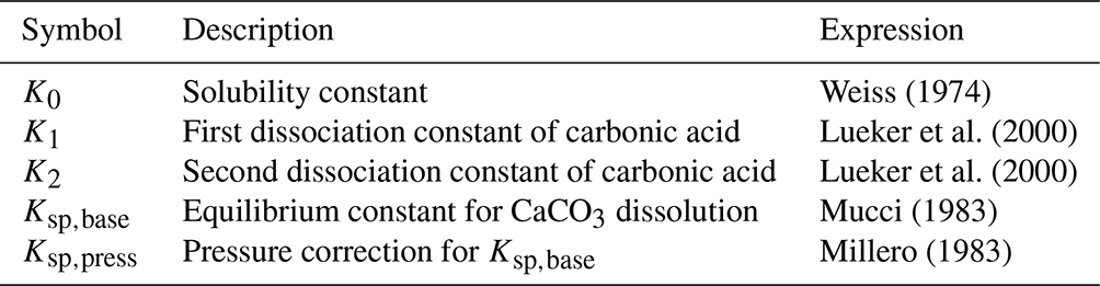
In this appendix values and descriptions of the parameters in the extended SCP-M are given. In Tables A1 to A3 the parameter values used in our model are presented. The values presented here are for the pre-industrial configuration. The parameter values that are different in the Last Glacial Maximum configuration are presented in Table 1. All parameter values, except the biological efficiency (ϵ) parameters, are taken from the SCP-M. The biological efficiency parameters have been fitted such that Z in Eq. (8a–d) is equal to Zbase under the original parameter values in the SCP-M. When determining the value of ϵ2,base, we also took the effect of the biological production in the North Pacific into account, which leads to a value of . In Table A4 we also present the literature where the expressions for the equilibrium constants were taken from.
Table A1Symbol (column 1), description (column 2), value (column 3), and units (column 4) of the general parameters used in our model.
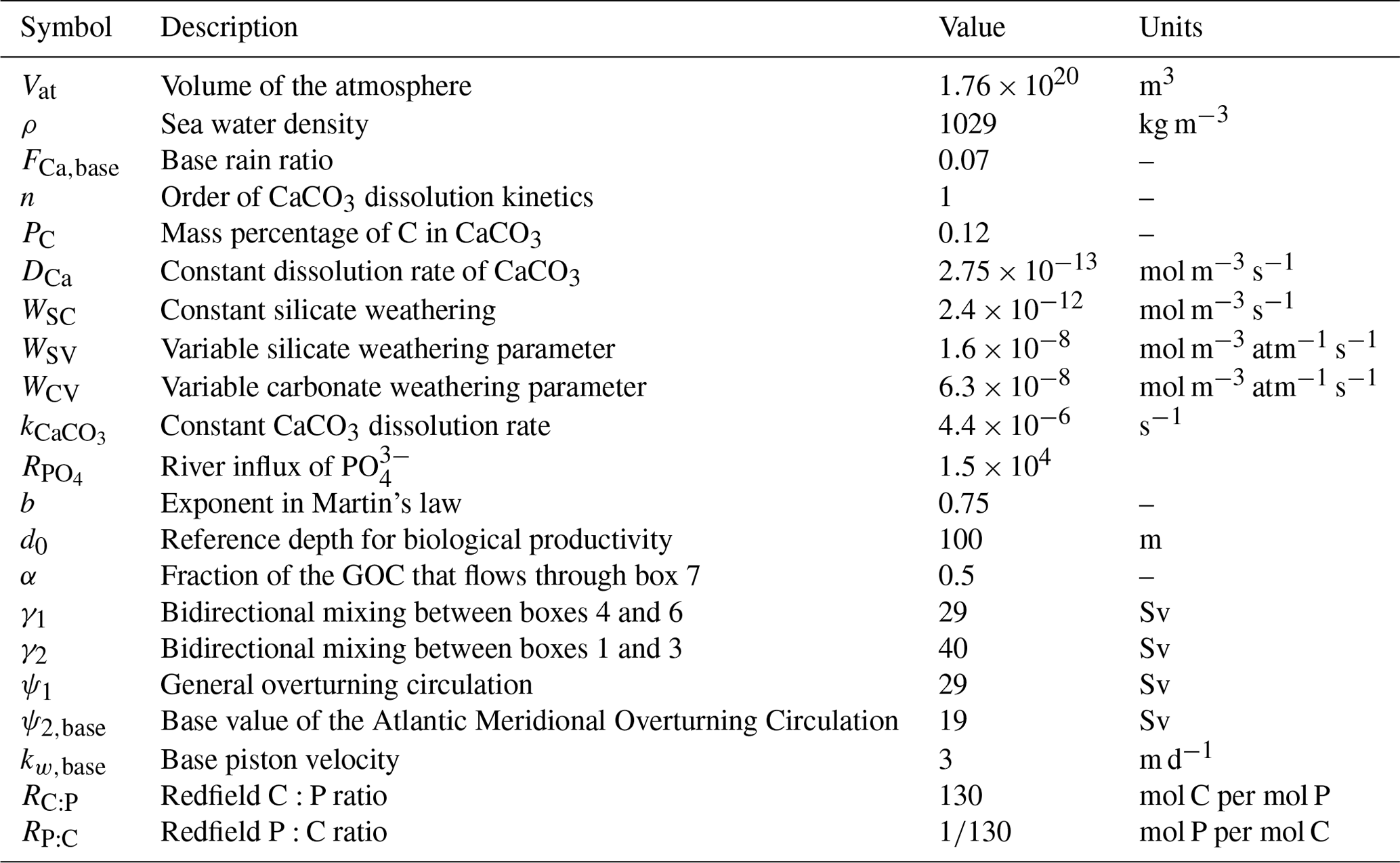
Table A2Symbol (column 1), description (column 2), value (column 3), and units (column 4) of parameters concerning the dimensions of the boxes used in our model.
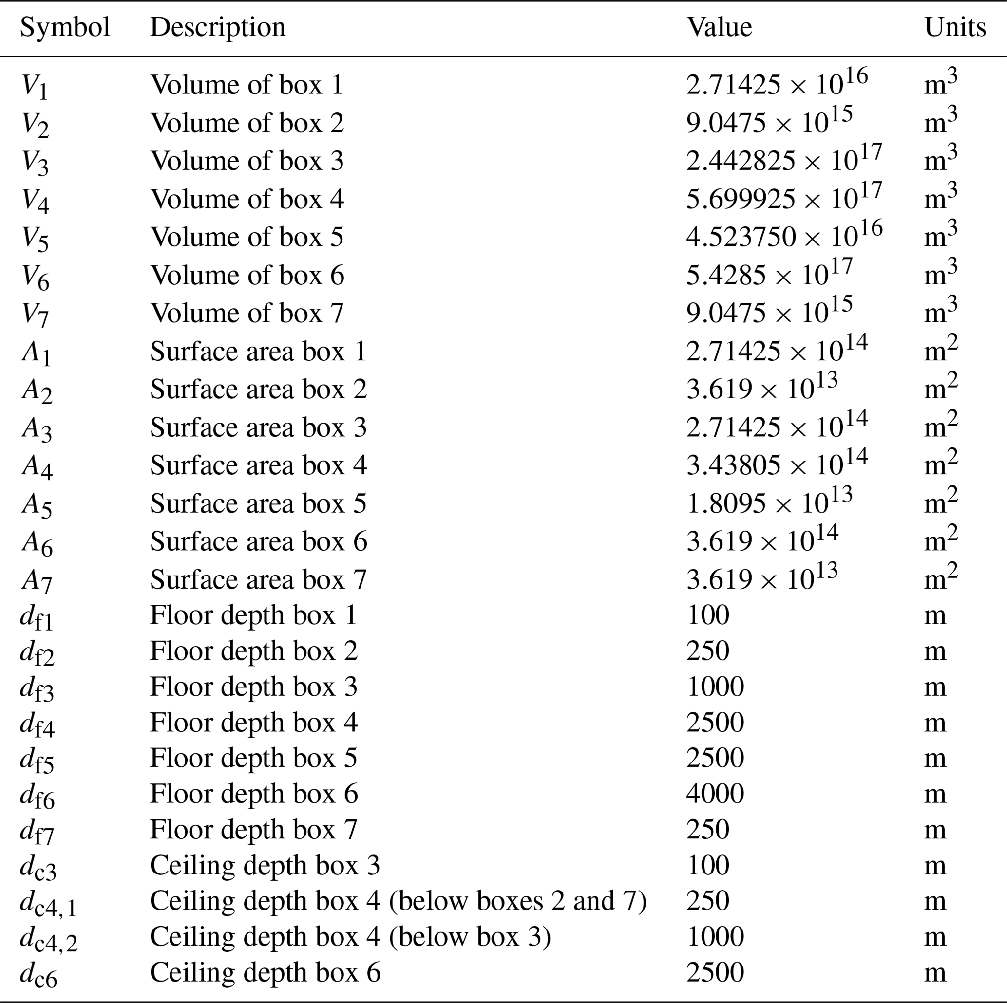
Table A3Symbol (column 1), description (column 2), value (column 3), and units (column 4) of the other parameters used in our model.
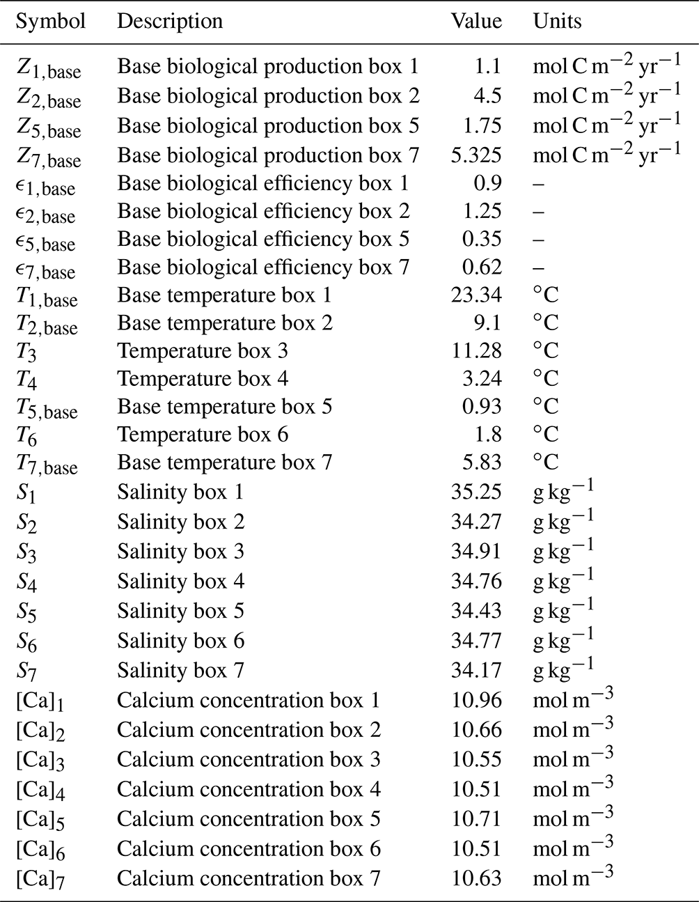
Table A4The symbols and description of the equilibrium constants are presented in the first two columns. The third column presents the source of the used expression.
The original version of the SCP-M is available at https://doi.org/10.5281/zenodo.1310161 (O'Neill et al., 2018), and the AUTO implementation is available at https://doi.org/10.5281/zenodo.4972553 (Boot et al., 2021). AUTO can be downloaded from https://sourceforge.net/projects/auto-07p/ (Doedel et al., 2022).
DB and HD designed the study and constructed the AUTO version of the SCP-M. DB obtained and analyzed all the results. DB and HD wrote the first version of the paper; all authors contributed to the writing of the final paper.
The contact author has declared that neither they nor their co-authors have any competing interests.
Publisher's note: Copernicus Publications remains neutral with regard to jurisdictional claims in published maps and institutional affiliations.
This research has been supported by the Netherlands Earth System Science Centre (grant no. 024.002.001).
This paper was edited by Kirsten Zickfeld and reviewed by two anonymous referees.
Archer, D., Kheshgi, H., and Maier-Reimer, E.: Multiple timescales for neutralization of fossil fuel CO2, Geophys. Res. Lett., 24, 405–408, https://doi.org/10.1029/97GL00168, 1997. a, b
Bakker, P., Schmittner, A., Lenaerts, J. T. M., Abe-Ouchi, A., Bi, D., van den Broeke, M. R., Chan, W.-L., Hu, A., Beadling, R. L., Marsland, S. J., Mernild, S. H., Saenko, O. A., Swingedouw, D., Sullivan, A., and Yin, J.: Fate of the Atlantic Meridional Overturning Circulation: Strong decline under continued warming and Greenland melting, Geophys. Res. Lett., 43, 12252–12260, https://doi.org/10.1002/2016GL070457, 2016. a
Barker, S. and Elderfield, H.: Foraminiferal Calcification Response to Glacial-Interglacial Changes in Atmospheric CO2, Science, 297, 833–836, https://doi.org/10.1126/science.1072815, 2002. a
Bauska, T. K., Marcott, S. A., and Brook, E. J.: Abrupt changes in the global carbon cycle during the last glacial period, Nat. Geosci., 14, 91–96, https://doi.org/10.1038/s41561-020-00680-2, 2021. a
Boot, D., Von der Heydt, A. S., and Dijkstra, H. A.: SCPM-AUTO-ESD, Zenodo [code and data set], https://doi.org/10.5281/zenodo.4972553, 2021. a
Cael, B. B., Bisson, K., and Follows, M. J.: How have recent temperature changes affected the efficiency of ocean biological carbon export?, Limnol. Oceanogr. Lett., 2, 113–118, https://doi.org/10.1002/lol2.10042, 2017. a
Cole, C., Finch, A. A., Hintz, C., Hintz, K., and Allison, N.: Effects of seawater pCO2 and temperature on calcification and productivity in the coral genus Porites spp.: an exploration of potential interaction mechanisms, Coral Reefs, 37, 471–481, https://doi.org/10.1007/s00338-018-1672-3, 2018. a
Doedel, E. J., Paffenroth, R. C., Champneys, A. C., Fairgrieve, T. F., Kuznetsov, Y. A., Oldeman, B. E., Sandstede, B., and Wang, X. J.: AUTO-07p: Continuation and Bifurcation Software for Ordinary Differential Equations, https://www.macs.hw.ac.uk/~gabriel/auto07/auto.html (last access: 27 June 2022), 2007. a
Doedel, E. J., Paffenroth, R. C., Champneys, A. C., Fairgrieve, T. F., Kuznetsov, Y. A., Oldeman, B. E., Sandstede, B., and Wang, X. J.: AUTO-07p, https://sourceforge.net/projects/auto-07p/, last access: 27 June 2022. a
Duplessy, J. C., Shackleton, N. J., Fairbanks, R. G., Labeyrie, L., Oppo, D., and Kallel, N.: Deepwater source variations during the last climatic cycle and their impact on the global deepwater circulation, Paleoceanography, 3, 343–360, https://doi.org/10.1029/PA003i003p00343, 1988. a
Follows, M. J., Ito, T., and Dutkiewicz, S.: On the solution of the carbonate chemistry system in ocean biogeochemistry models, Ocean Model., 12, 290–301, https://doi.org/10.1016/j.ocemod.2005.05.004, 2006. a, b
Friedlingstein, P., O'Sullivan, M., Jones, M. W., Andrew, R. M., Hauck, J., Olsen, A., Peters, G. P., Peters, W., Pongratz, J., Sitch, S., Le Quéré, C., Canadell, J. G., Ciais, P., Jackson, R. B., Alin, S., Aragão, L. E. O. C., Arneth, A., Arora, V., Bates, N. R., Becker, M., Benoit-Cattin, A., Bittig, H. C., Bopp, L., Bultan, S., Chandra, N., Chevallier, F., Chini, L. P., Evans, W., Florentie, L., Forster, P. M., Gasser, T., Gehlen, M., Gilfillan, D., Gkritzalis, T., Gregor, L., Gruber, N., Harris, I., Hartung, K., Haverd, V., Houghton, R. A., Ilyina, T., Jain, A. K., Joetzjer, E., Kadono, K., Kato, E., Kitidis, V., Korsbakken, J. I., Landschützer, P., Lefèvre, N., Lenton, A., Lienert, S., Liu, Z., Lombardozzi, D., Marland, G., Metzl, N., Munro, D. R., Nabel, J. E. M. S., Nakaoka, S.-I., Niwa, Y., O'Brien, K., Ono, T., Palmer, P. I., Pierrot, D., Poulter, B., Resplandy, L., Robertson, E., Rödenbeck, C., Schwinger, J., Séférian, R., Skjelvan, I., Smith, A. J. P., Sutton, A. J., Tanhua, T., Tans, P. P., Tian, H., Tilbrook, B., van der Werf, G., Vuichard, N., Walker, A. P., Wanninkhof, R., Watson, A. J., Willis, D., Wiltshire, A. J., Yuan, W., Yue, X., and Zaehle, S.: Global Carbon Budget 2020, Earth Syst. Sci. Data, 12, 3269–3340, https://doi.org/10.5194/essd-12-3269-2020, 2020. a
Ganachaud, A. and Wunsch, C.: Improved estimates of global ocean circulation, heat transport and mixing from hydrographic data, Nature, 408, 453–457, https://doi.org/10.1038/35044048, 2000. a
Gottschalk, J., Battaglia, G., Fischer, H., Frölicher, T. L., Jaccard, S. L., Jeltsch-Thömmes, A., Joos, F., Köhler, P., Meissner, K. J., Menviel, L., Nehrbass-Ahles, C., Schmitt, J., Schmittner, A., Skinner, L. C., and Stocker, T. F.: Mechanisms of millennial-scale atmospheric CO2 change in numerical model simulations, Quaternary Sci. Rev., 220, 30–74, https://doi.org/10.1016/j.quascirev.2019.05.013, 2019. a, b
Gregory, J. M., Dixon, K. W., Stouffer, R. J., Weaver, A. J., Driesschaert, E., Eby, M., Fichefet, T., Hasumi, H., Hu, A., Jungclaus, J. H., Kamenkovich, I. V., Levermann, A., Montoya, M., Murakami, S., Nawrath, S., Oka, A., Sokolov, A. P., and Thorpe, R. B.: A model intercomparison of changes in the Atlantic thermohaline circulation in response to increasing atmospheric CO2 concentration, Geophys. Res. Lett., 32, L12703, https://doi.org/10.1029/2005GL023209, 2005. a
Gruber, N., Landschützer, P., and Lovenduski, N. S.: The Variable Southern Ocean Carbon Sink, Annu. Rev. Mar. Sci., 11, 159–186, https://doi.org/10.1146/annurev-marine-121916-063407, 2019. a
Huiskamp, W. N. and Meissner, K. J.: Oceanic carbon and water masses during the Mystery Interval: A model-data comparison study, Paleoceanography, 27, PA4206, https://doi.org/10.1029/2012PA002368, 2012. a
Jiang, X. and Yung, Y. L.: Global Patterns of Carbon Dioxide Variability from Satellite Observations, Annu. Rev. Earth Planet. Sci., 47, 225–245, https://doi.org/10.1146/annurev-earth-053018-060447, 2019. a
Kwon, E. Y. and Primeau, F.: Optimization and sensitivity of a global biogeochemistry ocean model using combined in situ DIC, alkalinity, and phosphate data, J. Geophys. Res.-Oceans, 113, C08011, https://doi.org/10.1029/2007JC004520, 2008. a
Lueker, T. J., Dickson, A. G., and Keeling, C. D.: Ocean pCO2 calculated from dissolved inorganic carbon, alkalinity, and equations for K1 and K2: validation based on laboratory measurements of CO2 in gas and seawater at equilibrium, Mar. Chem., 70, 105–119, https://doi.org/10.1016/S0304-4203(00)00022-0, 2000. a, b
Marchal, O., Stocker, T. F., and Joos, F.: Impact of oceanic reorganizations on the ocean carbon cycle and atmospheric carbon dioxide content, Paleoceanography, 13, 225–244, https://doi.org/10.1029/98PA00726, 1998. a
Mariotti, V., Bopp, L., Tagliabue, A., Kageyama, M., and Swingedouw, D.: Marine productivity response to Heinrich events: a model-data comparison, Clim. Past, 8, 1581–1598, https://doi.org/10.5194/cp-8-1581-2012, 2012. a
Martin, J. H., Knauer, G. A., Karl, D. M., and Broenkow, W. W.: VERTEX: carbon cycling in the northeast Pacific, Deep-Sea Res, Pt. A, 34, 267–285, https://doi.org/10.1016/0198-0149(87)90086-0, 1987. a
Menviel, L., Timmermann, A., Mouchet, A., and Timm, O.: Meridional reorganizations of marine and terrestrial productivity during Heinrich events, Paleoceanography, 23, PA1203, https://doi.org/10.1029/2007PA001445, 2008. a
Menviel, L., England, M. H., Meissner, K. J., Mouchet, A., and Yu, J.: Atlantic-Pacific seesaw and its role in outgassing CO2 during Heinrich events, Paleoceanography, 29, 58–70, https://doi.org/10.1002/2013PA002542, 2014. a, b
Millero, F. J.: Chapter 43 – Influence of Pressure on Chemical Processes in the Sea, Academic Press, 1–88, https://doi.org/10.1016/B978-0-12-588608-6.50007-9, 1983. a
Mucci, A.: The solubility of calcite and aragonite in seawater at various salinities, temperatures, and one atmosphere total pressure, Am. J. Sci., 283, 780–799, https://doi.org/10.2475/ajs.283.7.780, 1983. a
Muller, R. A. and MacDonald, G. J.: Ice Ages and Astronomical Causes, Springer-Verlag, ISBN 978-3-540-43779-6, 2000. a
Munday, D. R., Johnson, H. L., and P, M. D.: Impacts and effects of mesoscale ocean eddies on ocean carbon storage and atmospheric pCO2, Global Biogeochem. Cy., 28, 877–896, https://doi.org/10.1002/2014GB004836, 2014. a
Munhoven, G.: Mathematics of the total alkalinity–pH equation – pathway to robust and universal solution algorithms: the SolveSAPHE package v1.0.1 Geosci. Model Dev., 6, 1367–1388, https://doi.org/10.5194/gmd-6-1367-2013, 2013. a, b, c, d
Nielsen, S. B., Jochum, M., Pedro, J. B., Eden, C., and Nuterman, R.: Two-Timescale Carbon Cycle Response to an AMOC Collapse, Paleoceanogr. Paleocl., 34, 511–523, https://doi.org/10.1029/2018PA003481, 2019. a, b
O'Neill, C. M., Hogg, A. M., Ellwood, M. J., Opdyke, B. N., and Eggins, S. M.: [simple carbon project] model (V1.0), Zenodo [code], https://doi.org/10.5281/zenodo.1310161, 2018. a
O'Neill, C. M., Hogg, A. M., Ellwood, M. J., Eggins, S. M., and Opdyke, B. N.: The [simple carbon project] model v1.0, Geosci. Model Dev., 12, 1541–1572, https://doi.org/10.5194/gmd-12-1541-2019, 2019. a, b, c, d, e
Petit, J. R., Jouzel, J., Raynaud, D., Barkov, N. I., Barnola, J.-M., Basile, I., Bender, M., Chappellaz, J., Davis, M., Delaygue, G., Delmotte, M., Kotlyakov, V. M., Legrand, M., Lipenkov, V. Y., Lorius, C., Pépin, L., Ritz, C., Saltzman, E., and Stievenard, M.: Climate and atmospheric history of the past 420,000 years from the Vostok ice core, Antarctica, Nature, 399, 429–436, https://doi.org/10.1038/20859, 1999. a
Ridgwell, A., Hargreaves, J. C., Edwards, N. R., Annan, J. D., Lenton, T. M., Marsh, R., Yool, A., and Watson, A.: Marine geochemical data assimilation in an efficient Earth System Model of global biogeochemical cycling, Biogeosciences, 4, 87–104, https://doi.org/10.5194/bg-4-87-2007, 2007. a
Rothman, D. H.: Earth's carbon cycle: A mathematical perspective, B. Am. Math. Soc., 52, 47–64, https://doi.org/10.1090/S0273-0979-2014-01471-5, 2015. a
Rothman, D. H.: Characteristic disruptions of an excitable carbon cycle, P. Natl. Acad. Sci. USA, 116, 14813–14822, https://doi.org/10.1073/pnas.1905164116, 2019. a, b, c, d, e, f, g
Sabine, C. L., Feely, R. A., Gruber, N., Key, R. M., Lee, K., Bullister, J. L., Wanninkhof, R., Wong, C. S., Wallace, D. W. R., Tilbrook, B., Millero, F. J., Peng, T.-H., Kozyr, A., Ono, T., and Rios, A. F.: The Oceanic Sink for Anthropogenic CO2, Science, 305, 367–371, https://doi.org/10.1126/science.1097403, 2004. a
Sarmiento, J. L. . and Gruber, N. .: Ocean biogeochemical dynamics, xii, 503 pages, 8 pages of plates: illustrations (some color), maps (some color); 29 cm, Princeton University Press, Princeton, SE, ISBN 978-0-691-01707-5, 2006. a
Schmittner, A., Brook, E. J., and Ahn, J.: Impact of the ocean's Overturning circulation on atmospheric CO2, in: Ocean Circulation: Mechanisms and Impacts – Past and Future Changes of Meridional Overturning, edited by: Schmittner, A., Chiang, J. C. H., and Hemming, S. R., Wiley, https://doi.org/10.1029/173GM20, 2007. a
Talley, L. D.: Closure of the Global Overturning Circulation Through the Indian, Pacific, and Southern Oceans: Schematics and Transports, Oceanography, 26, 80–97, https://doi.org/10.5670/oceanog.2013.07, 2013. a
Toggweiler, J. R. and Russell, J.: Ocean circulation in a warming climate, Nature, 451, 286–288, https://doi.org/10.1038/nature06590, 2008. a, b
Vellinga, M. and Wood, R. A.: Global Climatic Impacts of a Collapse of the Atlantic Thermohaline Circulation, Climatic Change, 54, 251–267, https://doi.org/10.1023/A:1016168827653, 2002. a
Walker, J. C. and Kasting, J. F.: Effects of fuel and forest conservation on future levels of atmospheric carbon dioxide, Global Planet. Change, 97, 151–189, 1992. a
Wanninkhof, R.: Relationship between wind speed and gas exchange over the ocean, J. Geophys. Res.-Oceans, 97, 7373–7382, https://doi.org/10.1029/92JC00188, 1992. a
Weijer, W., Cheng, W., Drijfhout, S. S., Fedorov, A. V., Hu, A., Jackson, L. C., Liu, W., McDonagh, E. L., Mecking, J. V., and Zhang, J.: Stability of the Atlantic Meridional Overturning Circulation: A Review and Synthesis, J. Geophys. Res.-Oceans, 124, 5336–5375, https://doi.org/10.1029/2019JC015083, 2019. a, b
Weijer, W., Cheng, W., Garuba, O. A., Hu, A., and Nadiga, B. T.: CMIP6 Models Predict Significant 21st Century Decline of the Atlantic Meridional Overturning Circulation, Geophys. Res. Lett., 47, e2019GL086075, https://doi.org/10.1029/2019GL086075, 2020. a
Weiss, R. F.: Carbon dioxide in water and seawater: the solubility of a non-ideal gas, Mar. Chem., 2, 203–215, https://doi.org/10.1016/0304-4203(74)90015-2, 1974. a
Williams, R. G. and Follows, M. J.: Ocean Dynamics and the Carbon Cycle: Principles and Mechanisms, Cambridge University Press, Cambridge, https://doi.org/10.1017/CBO9780511977817, 2011. a
Zeebe, R. E.: LOSCAR: Long-term Ocean-atmosphere-Sediment CArbon cycle Reservoir Model v2.0.4, Geosci. Model Dev., 5, 149–166, https://doi.org/10.5194/gmd-5-149-2012, 2012. a
Zeebe, R. E. and Westbroek, P.: A simple model for the CaCO3 saturation state of the ocean: The “Strangelove”, the “Neritan”, and the “Cretan” Ocean, Geochem. Geophy. Geosy., 4, 1104, https://doi.org/10.1029/2003GC000538, 2003. a
Zelinka, M. D., Myers, T. A., McCoy, D. T., Po-Chedley, S., Caldwell, P. M., Ceppi, P., Klein, S. A., and Taylor, K. E.: Causes of Higher Climate Sensitivity in CMIP6 Models, Geophys. Res. Lett., 47, e2019GL085782, https://doi.org/10.1029/2019GL085782, 2020. a, b
Zhu, J., Liu, Z., Zhang, J., and Liu, W.: AMOC response to global warming: dependence on the background climate and response timescale, Clim. Dynam., 44, 3449–3468, https://doi.org/10.1007/s00382-014-2165-x, 2015. a