The half-order energy balance equation – Part 2: The inhomogeneous HEBE and 2D energy balance models

In Part 1, I considered the zero-dimensional heat equation, showing quite generally that conductive–radiative surface boundary conditions lead to half-ordered derivative relationships between surface heat fluxes and temperatures: the half-ordered energy balance equation (HEBE). The real Earth, even when averaged in time over the weather scales (up to ≈ 10 d), is highly heterogeneous. In this Part 2, the treatment is extended to the horizontal direction. I first consider a homogeneous Earth but with spatially varying forcing on both a plane and on the sphere: the new equations are compared with the canonical 1D Budyko–Sellers equations. Using Laplace and Fourier techniques, I derive the generalized HEBE (the GHEBE) based on half-ordered space–time operators. I analytically solve the homogeneous GHEBE and show how these operators can be given precise interpretations.

I then consider the full inhomogeneous problem with horizontally varying diffusivities, thermal capacities, climate sensitivities, and forcings. For this I use Babenko's operator method, which generalizes Laplace and Fourier methods. By expanding the inhomogeneous space–time operator at both high and low frequencies, I derive 2D energy balance equations that can be used for macroweather forecasting, climate projections, and studying the approach to new (equilibrium) climate states when the forcings are all increased and held constant.

1 Introduction

In Part 1, I showed that when the surface of a body exchanges heat both conductively and radiatively, its flux depends on the half-order derivative of the surface temperature (Lovejoy, 2021). This implies that energy stored in the subsurface effectively has a huge power-law memory. This contrasts with the usual phenomenological assumption notably used in box models (including zero-dimensional global energy balance models) that the order of the derivative is an integer (one) and that, on the contrary, the memory is only exponential (short). The result directly followed by assuming that the continuum mechanics heat equation was obeyed and the depth of the media was of the order of a few diffusion depths; for the Earth, this is perhaps several hundred meters. The basic result was a classical application of the heat equation barely going beyond the results that Brunt (1932) already found “in any textbook”.

A consequence was that although Newton's law of cooling is obeyed, the temperature obeyed the half-order energy balance equation (HEBE) rather than the phenomenological first-order energy balance equation (EBE). When applied to the Earth, the HEBE and its implied long memory explain the success of both climate projections through 2100 (Hebert, 2017; Lovejoy et al., 2017; Hébert et al., 2020) and macroweather (monthly, seasonal) temperature forecasts (Lovejoy et al., 2015; Del Rio Amador and Lovejoy, 2019, 2021a, b). I also considered the responses to periodic forcings, showing that surface heat fluxes and temperatures are related by a complex thermal impedance (Z(ω), ω is the frequency). In the Earth system, Z(ω)=s(ω), where s(ω) is the complex climate sensitivity that is estimated from a simple semi-empirical model.

Although in Part 1 I discussed the classical 1D application of the heat equation to the Earth's latitudinal energy balance (Budyko–Sellers models, especially their ad hoc treatment of the surface boundary condition), the discussion was restricted to zero horizontal dimensions. In this Part 2, I first (Sect. 2) extend the Part 1 treatment to systems with homogeneous properties but with inhomogeneous forcings, first in the horizontal plane (Sect. 2.1, 2.2), then – following Budyko–Sellers – latitudinally varying on the sphere (Sect. 2.3). The homogeneous case is quite classical and can be treated with standard Laplace and Fourier techniques; it leads to the (horizontally) generalized HEBE: the GHEBE. Although the GHEBE has a more complex (space–time) fractional derivative operator that is unlike anything I know of in the literature, like the HEBE, it can nevertheless be given precise meaning via its Green's function.

In Sect. 3, I derive the inhomogeneous GHEBE and HEBE needed for applications. This is done by using Babenko's method (Babenko, 1986), which is essentially a generalization of Laplace and Fourier transform techniques. The challenge with Babenko's method is to interpret the inhomogeneous space–time fractional operators. Following Babenko, this is done using both high- and low-frequency expansions respectively corresponding to processes dominated by storage and horizontal heat transport. The long-time limit describes the new energy balance climate state that results when the forcing is increased everywhere and held fixed: for the model this corresponds to equilibrium. I also include several appendices focused on empirical parameter estimates (Appendix A), the implications for two-point and space–time temperature statistics (when the system is stochastically forced with internal variability; Appendix B), and finally (Appendix C) the changes needed to account for the Earth's spherical geometry, including the definition of fractional operators on the sphere.

2 The two-dimensional homogeneous heat equation

2.1 The homogeneous GHEBE

In Part 1 I recalled the heat equation for the time-varying temperature anomalies (T) with diffusive and (horizontal) effective advective velocity (v).

$$\begin{array}{}\text{(1)}& \left({\displaystyle \frac{\partial }{\partial t}}-{\mathit{\kappa }}_{\mathrm{v}}{\displaystyle \frac{{\partial }^{\mathrm{2}}}{\partial z^{\mathrm{2}}}}\right)T=-\mathit{v}\cdot {\mathrm{\nabla }}_{\mathrm{h}}T+{\mathit{\kappa }}_{\mathrm{h}}{\mathrm{\nabla }}_{\mathrm{h}}^{\mathrm{2}}T\end{array}$$

This is written in the still general form of Eq. (19) in Part 1. κ_h and κ_v are horizontal and vertical thermal diffusivities, z the vertical coordinate (pointing upwards, the Earth is z≤0), t the time, $\mathit{x}=(x,y)$ the horizontal coordinates, and ${\mathrm{\nabla }}_{\mathrm{h}}=\widehat{x}\partial /\partial x+\widehat{y}\partial /\partial y$ (the circumflexes indicate unit vectors). These equations must now be solved using the conductive–radiative surface boundary condition:

$$\begin{array}{}\text{(2)}& \left({\displaystyle \frac{T(\mathit{x},z,t)}{s}}+\mathit{\rho }c{\mathit{\kappa }}_{\mathrm{v}}{\displaystyle \frac{\partial T(\mathit{x},z,t)}{\partial z}}\right){|}_{z=\mathrm{0}}=F(x,t),\end{array}$$

where ρ and c represent the fluid densities and specific heats, s is the climate sensitivity, and F is the anomaly forcing. The initial conditions are T= 0 at $z=-\mathrm{\infty }$ (all t) and $T(\mathit{x},z,t=\mathrm{0})=\mathrm{0}$ (Riemann–Liouville) or $T(\mathit{x},z,t=-\mathrm{\infty })=\mathrm{0}$ (Weyl).

In Part 1, I nondimensionalized the zero-dimensional homogeneous operators by nondimensionalizing time by the relaxation time $t\to t/\mathit{\tau }$ (with τ=κ_v(ρcs)²) and nondimensionalizing the vertical distance by the vertical diffusion depth: $z\to z/l_{\mathrm{v}}$ (with $l_{\mathrm{v}}={\left(\mathit{\tau }{\mathit{\kappa }}_{\mathrm{v}}\right)}^{\mathrm{1}/\mathrm{2}}$). Considering the full equation with advective and diffusive transport, we nondimensionalize the horizontal coordinates by the horizontal diffusion length $\mathit{x}\to \mathit{x}/l_{\mathrm{h}}$ (with $l_{\mathrm{h}}={\left(\mathit{\tau }{\mathit{\kappa }}_{\mathrm{h}}\right)}^{\mathrm{1}/\mathrm{2}})$ and use the nondimensional advection velocity $\mathit{\alpha }=\frac{\mathit{v}}{V}$ (with speed $V=\frac{l_{\mathrm{h}}}{\mathit{\tau }}$). If we now take s= 1 (equivalent to using dimensions of temperature for the forcing F), we obtain

$${\displaystyle }\left({\displaystyle \frac{{\partial }^{\mathrm{2}}}{\partial z^{\mathrm{2}}}}-\left({\displaystyle \frac{\partial }{\partial t}}+\left(-{\mathrm{\nabla }}_{\mathrm{h}}^{\mathrm{2}}\right)-\mathit{\alpha }\cdot {\mathrm{\nabla }}_{\mathrm{h}}\right)\right)T=\mathrm{0},$$

$$\begin{array}{}\text{(3)}& \begin{array}{l}{\left.\frac{\partial T}{\partial z}\right|}_{z=\mathrm{0}}+T\left(t,\mathit{x};\mathrm{0}\right)=F\left(t,\mathit{x}\right),\end{array}\end{array}$$

for the heat equation and the conductive–radiative surface boundary condition, respectively. For initial conditions such that T= 0 for t≤ 0, as in Part 1, I take Laplace transforms in time, but we now take Fourier transforms in the horizontal:

$$\begin{array}{}\text{(4)}& \begin{array}{rl}& \left({\displaystyle \frac{{\partial }^{\mathrm{2}}}{\partial z^{\mathrm{2}}}}-\left({\displaystyle \frac{\partial }{\partial t}}+\left(-{\mathrm{\nabla }}_{\mathrm{h}}^{\mathrm{2}}\right)-\mathit{\alpha }\cdot {\mathrm{\nabla }}_{\mathrm{h}}\right)\right)T=\mathrm{0}\\ & \stackrel{\mathrm{LT}\left(\mathrm{t}\right),\mathrm{FT}\left(x\right)}{\leftrightarrow }\left({\displaystyle \frac{d^{\mathrm{2}}}{\mathrm{d}{z}^{\mathrm{2}}}}-(p+k^{\mathrm{2}}-i\mathit{\alpha }\cdot \mathit{k})\right)\widehat{T}=\mathrm{0},\end{array}\end{array}$$

where FT is the Fourier transform in horizontal space and k is for the conjugate of x and $k=\left|\mathit{k}\right|$ (the vector modulus) with conjugate variable $r=\left|\mathit{x}\right|$ (as usual, ${\mathrm{\nabla }}_{\mathrm{h}}\stackrel{\mathrm{FT}}{\leftrightarrow }i\mathit{k}$). Fourier transforms in space are convenient for either infinite horizontal media or media with periodic horizontal boundary conditions. In Appendix C, I consider the changes needed to account for spherical geometry.

When $F\left(t,\mathit{x}\right)=\mathit{\delta }\left(t\right)\mathit{\delta }\left(\mathit{x}\right)$, the solution is $T\left(t,\mathit{x}\right)=G_{\mathit{\delta }}(t,\mathit{x})$ and $\widehat{T}(p,\mathit{k})={\widehat{G}}_{\mathit{\delta }}(p,\mathit{k})$, where G_δ is the impulse (Dirac) response Green's function (Part 1, Eq. 30). From Eq. (4), we see that this is the same as the zero-dimensional equation (Eq. 24, Part 1) but with $p\to p+k^{\mathrm{2}}-i\mathit{\alpha }\cdot \mathit{k}$, i.e., for the corresponding Green's function,

$$\begin{array}{}\text{(5)}& \widehat{G_{\mathit{\delta }}}\left(p,\mathit{k};z\right)=\widehat{G_{\mathit{\delta }}}\left(p+k^{\mathrm{2}}-i\mathit{\alpha }\cdot \mathit{k};z\right).\end{array}$$

A note on notation: the first argument is time, with the vertical separated by a semicolon. When there is a horizontal coordinate it comes after time, before the semicolon. With this notation, the right-hand side of Eq. (5) is the LT of the zero-dimensional (time–depth) Green's function G_δ(t;z), and the left-hand side is the Laplace (time) and Fourier transform (horizontal, space).

We can now use the basic Laplace shift property,

$$\begin{array}{}\text{(6)}& e^{(-k^{\mathrm{2}}+i\mathit{\alpha }\cdot \mathit{k})t}{G}_{\mathit{\delta }}(t;z)\stackrel{\mathrm{LT}\left(t\right)}{\leftrightarrow }{\widehat{G}}_{\mathit{\delta }}(p+k^{\mathrm{2}}-i\mathit{\alpha }\cdot \mathit{k};z),\end{array}$$

to conclude that

$$\begin{array}{}\text{(7)}& {\widehat{G}}_{\mathit{\delta }}(t,\mathit{k};z)=e^{(-k^{\mathrm{2}}+i\mathit{\alpha }\cdot \mathit{k})t}{G}_{\mathit{\delta }}(t;z).\end{array}$$

Decomposing this into a circularly symmetric diffusion part ${\widehat{G}}_{\mathit{\delta },\mathrm{dif}}\left(t,\mathit{k};z\right)$ and a factor e^ik⋅αt that shifts phases, we obtain

$$\begin{array}{}\text{(8)}& \begin{array}{rl}{\widehat{G}}_{\mathit{\delta }}(t,\mathit{k};z)& =e^{(i\mathit{k}\cdot \mathit{\alpha }t)}{\widehat{G}}_{\mathit{\delta },\mathrm{dif}}(t,\mathit{k};z);\\ & {\widehat{G}}_{\mathit{\delta },\mathrm{dif}}(t,\mathit{k};z)=e^{-k^{\mathrm{2}}t}{G}_{\mathit{\delta }}(t;z).\end{array}\end{array}$$

By circular symmetry of ${\widehat{G}}_{\mathit{\delta },\mathrm{dif}}\left(t,\mathit{k};z\right)$, its inverse (2D) Fourier transform reduces to an inverse Hankel transform (HT). Using

$$\begin{array}{}\text{(9)}& {\displaystyle \frac{e^{-r^{\mathrm{2}}/\left(\mathrm{4}t\right)}}{\mathrm{2}t}}\stackrel{\mathrm{HT}}{\leftrightarrow }{e}^{-k^{\mathrm{2}}t},\end{array}$$

we therefore obtain the following for the diffusive part of the surface impulse response (i.e., the response with source spatial forcing $\mathit{\delta }\left(\mathit{x}\right)=\mathit{\delta }\left(r\right)/\left(\mathrm{2}\mathit{\pi }r\right))$:

$$\begin{array}{}\text{(10)}& G_{\mathit{\delta },\mathrm{dif}}\left(t,r;z\right)={\displaystyle \frac{e^{-r^{\mathrm{2}}/\left(\mathrm{4}t\right)}}{\mathrm{2}t}}{G}_{\mathit{\delta }}\left(t;z\right),\end{array}$$

where G_δ(t;z) is the zero-dimensional impulse response. If needed, its integral representation is given in Eq. (34) in Part 1. The last step is to take into account the advective term associated with the phase shift k⋅αt. For this final step, use the Fourier shift theorem to obtain

$$\begin{array}{}\text{(11)}& G_{\mathit{\delta }}\left(t,\mathit{x};z\right)=G_{\mathit{\delta },\mathrm{dif}}(t,|\mathit{x}-\mathit{\alpha }t|;z)={\displaystyle \frac{e^{-|\mathit{x}-\mathit{\alpha }t{|}^{\mathrm{2}}/(\mathrm{4}t)}}{\mathrm{2}t}}{G}_{\mathit{\delta }}(t;z).\end{array}$$

This is the general result for the diffusive–advective transport part of the spatially homogeneous case. As expected, the advective transport simply displaces the center of the impulse response with nondimensional velocity α. As usual, the solutions for arbitrary forcing F(t,x) can be obtained by convolution.

For the surface we obtain simpler expressions for the diffusive impulse and step responses (see Eq. 35, Part 1).

$${\displaystyle }{G}_{\mathit{\delta },\mathrm{dif}}\left(t,r;\mathrm{0}\right)={\displaystyle \frac{e^{-r^{\mathrm{2}}/\left(\mathrm{4}t\right)}}{\mathrm{2}t}}\left({\displaystyle \frac{\mathrm{1}}{\sqrt{\mathit{\pi }t}}}-e^t\mathrm{erfc}\sqrt{t}\right)$$

$$\begin{array}{}\text{(12)}& \begin{array}{rl}{G}_{\mathrm{\Theta },\mathrm{dif}}& \left(t,r;\mathrm{0}\right)=\underset{\mathrm{0}}{\overset{t}{\int }}{G}_{\mathit{\delta },\mathrm{dif}}\left(t,r;\mathrm{0}\right)\mathrm{d}t\\ & ={\displaystyle \frac{\mathrm{1}}{r}}\mathrm{erfc}\left({\displaystyle \frac{r}{\mathrm{2}\sqrt{t}}}\right)-\underset{\mathrm{0}}{\overset{t}{\int }}{\displaystyle \frac{e^{-\frac{r^{\mathrm{2}}}{\mathrm{4}s}+s}}{\mathrm{2}s}}\mathrm{erfc}\left(s^{\mathrm{1}/\mathrm{2}}\right)\mathrm{d}s\end{array}\end{array}$$

From these, the general surface results including advection are obtained with $r\to |\mathit{x}-\mathit{\alpha }t|$, i.e., $G_{\mathit{\delta }}(t,\mathit{x};\mathrm{0})=G_{\mathit{\delta },\mathrm{dif}}(t,|\mathit{x}-\mathit{\alpha }t|;\mathrm{0})$.

Since the advection term has this simple consequence, below, take α=0, considering only diffusive transport; advection can easily be included if needed (i.e., below, take $G_{\mathit{\delta }}\left(t,r;\mathrm{0}\right)=G_{\mathit{\delta },\mathrm{dif}}\left(t,r;\mathrm{0}\right))$.

To better understand the impulse response, Fig. 1 shows this surface $G_{\mathit{\delta }}\left(t,r;\mathrm{0}\right)$ for various radial distances r, and Fig. 2 shows the corresponding time dependence of the time integral of G_δ; the unit step response is G_Θ for various distances r, illustrating the power-law approach to equilibrium at large t (discussed in Sect. 2.2). The corresponding long-time (t≫1) short-distance (r≪1) expansions are as follows.

$$G_{\mathit{\delta }}\left(t,r;\mathrm{0}\right)\approx {\displaystyle \frac{t^{-\mathrm{5}/\mathrm{2}}}{\mathrm{4}\sqrt{\mathit{\pi }}}}-{\displaystyle \frac{\left(\mathrm{6}+r^{\mathrm{2}}\right)}{\mathrm{16}\sqrt{\mathit{\pi }}}}{t}^{-\mathrm{7}/\mathrm{2}}+O\left(t^{-\mathrm{9}/\mathrm{2}}\right)$$

$$\begin{array}{}\text{(13)}& G_{\mathrm{\Theta }}\left(t,r;\mathrm{0}\right)\approx G_{\mathrm{eq},\mathit{\delta }}\left(r;\mathrm{0}\right)-{\displaystyle \frac{t^{-\mathrm{3}/\mathrm{2}}}{\mathrm{6}\sqrt{\mathit{\pi }}}}+{\displaystyle \frac{\left(\mathrm{6}+r^{\mathrm{2}}\right)}{\mathrm{40}\sqrt{\mathit{\pi }}}}{t}^{-\mathrm{5}/\mathrm{2}}+O\left(t^{-\mathrm{7}/\mathrm{2}}\right)\end{array}$$

$G_{\mathrm{eq},\mathit{\delta }}\left(r,\mathrm{0}\right)$ is the Green's function for the (spatial Dirac) “hot spot” equilibrium response discussed below (Eq. 20). Note that the leading term in $G_{\mathit{\delta }}\left(t,r;\mathrm{0}\right)$ is independent of r, and the leading term in the approach to equilibrium $G_{\mathrm{\Theta }}\left(t,r;\mathrm{0}\right)$ is also independent of r.

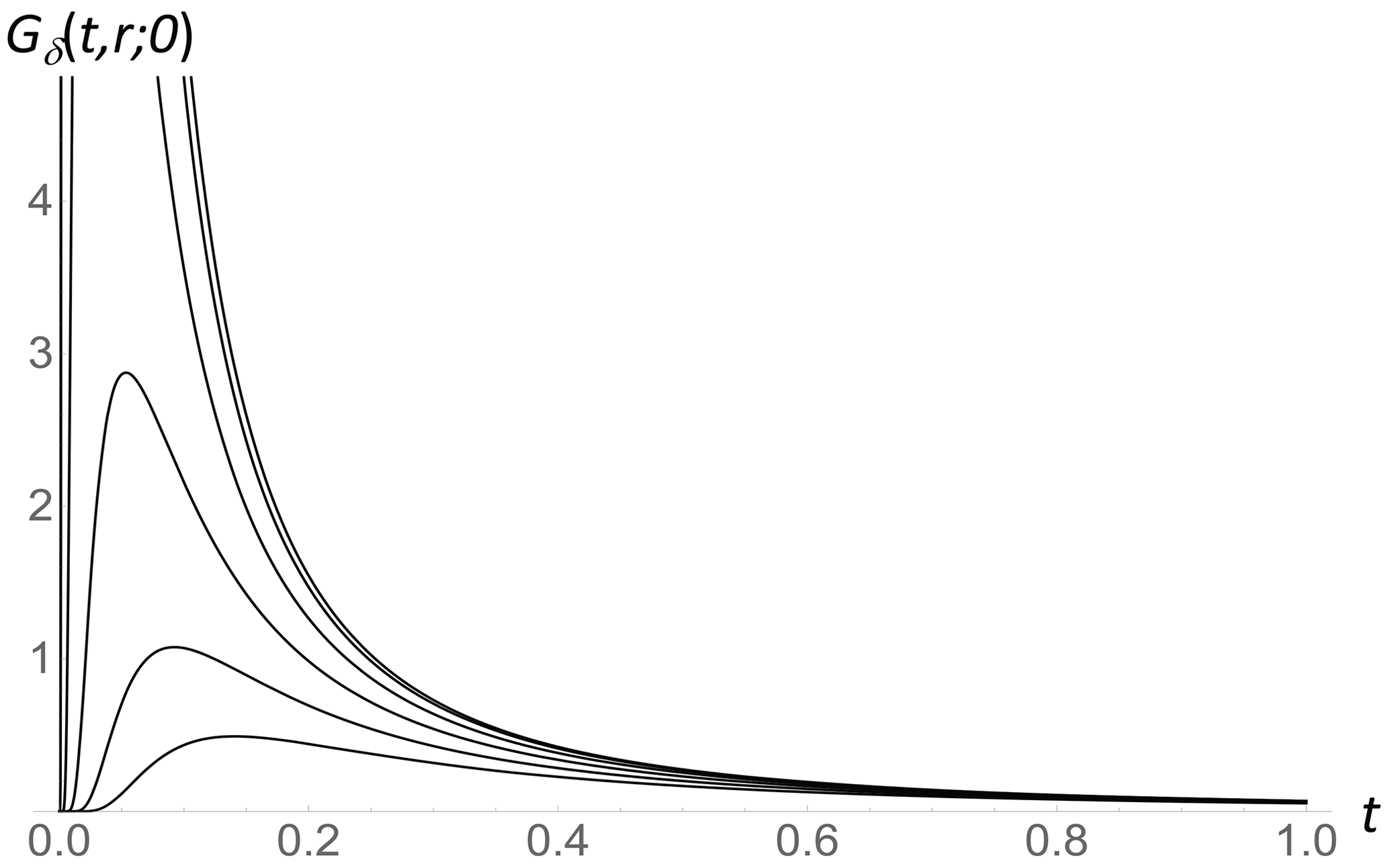
Figure 1 The surface impulse response function ($G_{\mathit{\delta }}\left(t,r;\mathrm{0}\right)$ in Eq. 12, i.e., Dirac in time and Dirac in space) as a function of nondimensional time (t) for nondimensional distance from the source increasing from r= 0 (top) to r= 1 in steps of 0.2 (top to bottom).

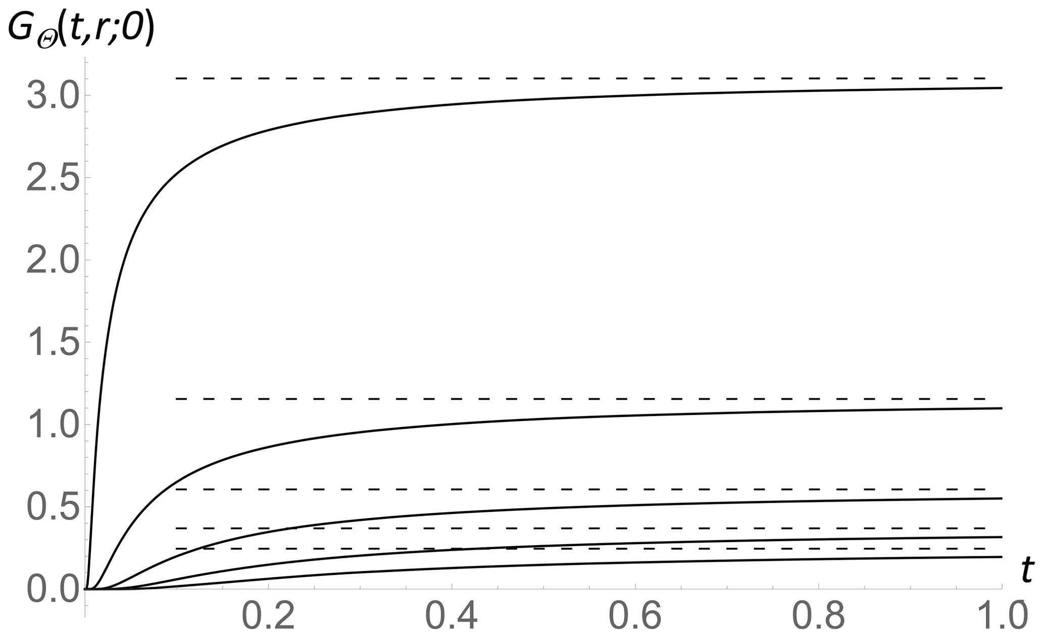
Figure 2 The surface step response (time) and Dirac (space) function ($G_{\mathrm{\Theta }}\left(t,r;\mathrm{0}\right)$, Eq. 12) as a function of nondimensional time; each curve is for a different nondimensional distance from the source increasing from r= 0.2 (top) to r= 1 in steps of 0.2 (top to bottom). At each distance r, the temperature approaches equilibrium (= G_therm,δ(r), Eq. 21) at large t (shown by dashed horizontal lines).

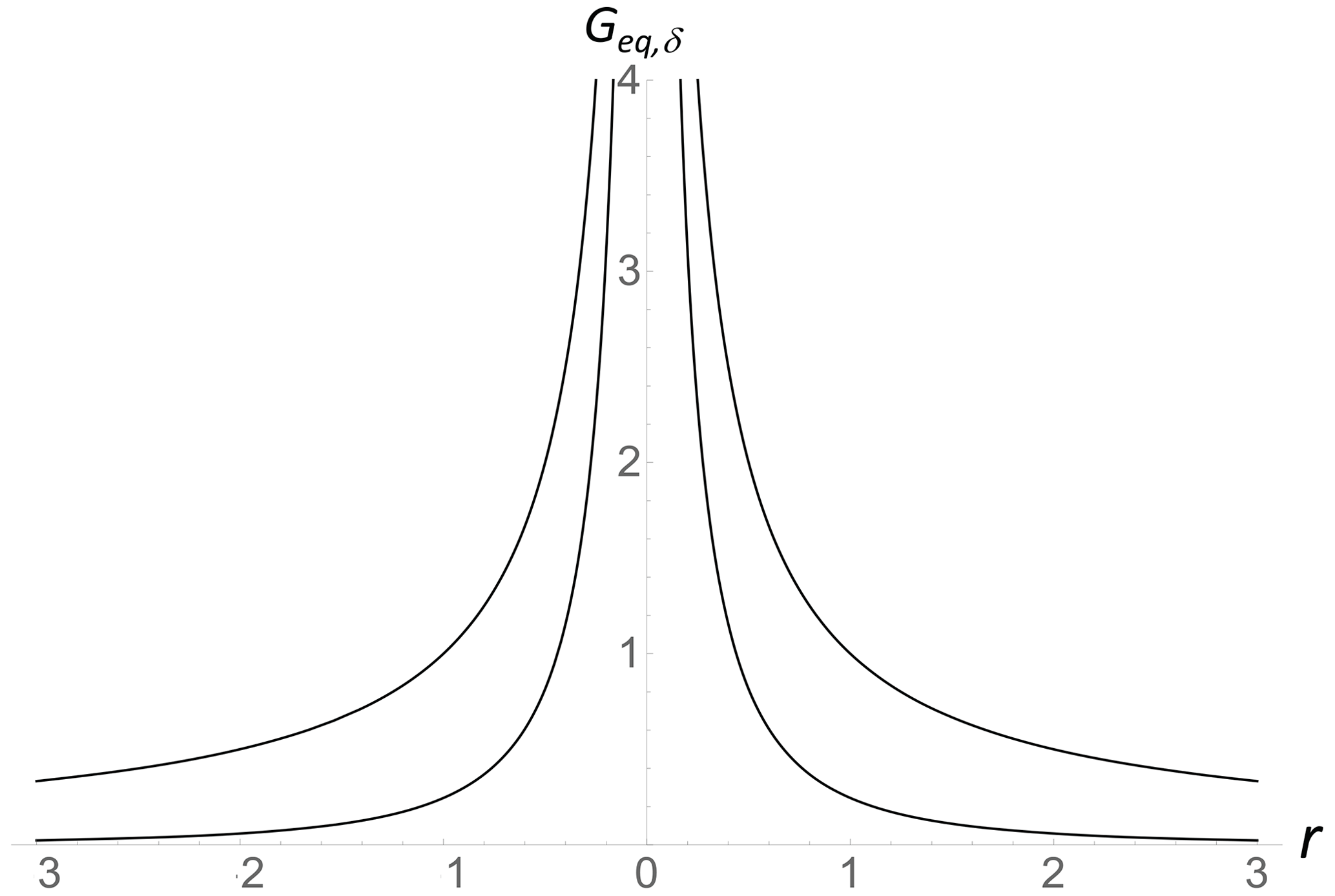
Figure 3 A comparison of the spatial impulse response Green's functions for equilibrium with surface forcing via conduction only; i.e., ${\left.\frac{\partial T_{\mathrm{eq}}}{\partial z}\right|}_{z=\mathrm{0}}=\mathit{\delta }\left(\mathit{x}\right)$ with no radiation; top $=r^{-\mathrm{1}}$ and bottom the same but with conduction–radiative forcing via the surface BC $\left({\left.\frac{\partial T_{\mathrm{eq}}}{\partial z}\right|}_{z=\mathrm{0}}+T\left(r;\mathrm{0}\right)=\mathit{\delta }\left(\mathit{x}\right)\right)$ that is asymptotically $\approx r^{-\mathrm{3}}$ (Eq. 22).

Just as the zero-dimensional HEBE was derived by showing that it had the same Green's function as the z= 0 transport equation Green's function, we can likewise derive the homogeneous generalized half-order energy balance equation (GHEBE), which is the space–time surface equation whose Green's function is given in Eq. (12). Following the derivation of the HEBE (Part 1 Eq. 29) and replacing $p\to p+k^{\mathrm{2}}-i\mathit{\alpha }\cdot \mathit{k}$, we obtain

$$\begin{array}{}\text{(14)}& {\widehat{G}}_{\mathit{\delta }}(p,\mathit{k};z)={\displaystyle \frac{e^{\sqrt{p+k^{\mathrm{2}}-i\mathit{\alpha }\cdot \mathit{k}z}}}{\sqrt{p+k^{\mathrm{2}}-i\mathit{\alpha }\cdot \mathit{k}}+\mathrm{1}}}.\end{array}$$

Hence, for z= 0,

$$\begin{array}{}\text{(15)}& \begin{array}{rl}& \left[{\left({\displaystyle \frac{\partial }{\partial t}}+\left(-{\mathrm{\nabla }}_{\mathrm{h}}^{\mathrm{2}}\right)-i\mathit{\alpha }\cdot {\mathrm{\nabla }}_{\mathrm{h}}\right)}^{\mathrm{1}/\mathrm{2}}+\mathrm{1}\right]G_{\mathit{\delta }}(t,\mathit{x};\mathrm{0})=\mathit{\delta }\left(t\right)\mathit{\delta }\left(\mathit{x}\right)\\ & \stackrel{\mathrm{LT}\left(t\right),\mathrm{FT}\left(x\right)}{\leftrightarrow }\left(\sqrt{p+k^{\mathrm{2}}-i\mathit{\alpha }\cdot \mathit{k}}+\mathrm{1}\right){\widehat{G}}_{\mathit{\delta }}(p,\mathit{k};\mathrm{0})=\mathrm{1}.\end{array}\end{array}$$

The left-hand equation is the homogeneous GHEBE whose Green's function is given by Eq. (12). We have therefore found a surprisingly simple explicit formula for the (inverse) half-order space–time GHEBE operator:

$$\begin{array}{}\text{(16)}& {\left[{\left({\displaystyle \frac{\partial }{\partial t}}+\left(-{\mathrm{\nabla }}_{\mathrm{h}}^{\mathrm{2}}\right)-i\mathit{\alpha }\cdot {\mathrm{\nabla }}_{\mathrm{h}}\right)}^{\mathrm{1}/\mathrm{2}}+\mathrm{1}\right]}^{-\mathrm{1}}\stackrel{\mathrm{LT}\left(t\right),\mathrm{FT}\left(x\right)}{\leftrightarrow }{G}_{\mathit{\delta }}(t,\mathit{x};\mathrm{0})*,\end{array}$$

where * indicates convolution. This allows a precise interpretation of the half-order operator. Therefore, the dimensional homogeneous GHEBE and its full solution are as follows.

$$\begin{array}{}\text{(17)}& \begin{array}{rl}(\mathit{\tau }{\displaystyle \frac{\partial }{\partial t}}& +\left(-l_{\mathrm{h}}^{\mathrm{2}}{\mathrm{\nabla }}_{\mathrm{h}}^{\mathrm{2}}\right)-i{l}_{\mathrm{h}}\mathit{\alpha }\cdot {\mathrm{\nabla }}_{\mathrm{h}}{)}^{\mathrm{1}/\mathrm{2}}{T}_{\mathrm{s}}(t,\mathit{x})+T_{\mathrm{s}}(t,\mathit{x})\\ & =sF(t,\mathit{x}),\end{array}\end{array}$$

and the solution is

$$\begin{array}{}\text{(18)}& \begin{array}{rl}{T}_{\mathrm{s}}& (t,\mathit{x})=s\underset{\mathrm{surf}}{\int }\underset{\mathrm{0}}{\overset{t}{\int }}{G}_{\mathit{\delta }}\left({\displaystyle \frac{t-t^{\prime }}{\mathit{\tau }}},{\displaystyle \frac{|\mathit{x}-{\mathit{x}}^{\prime }|}{l_{\mathrm{h}}}};\mathrm{0}\right)F(t^{\prime },{\mathit{x}}^{\prime }){\displaystyle \frac{\mathrm{d}{t}^{\prime }}{\mathit{\tau }}}{\displaystyle \frac{\mathrm{d}{\mathit{x}}^{\prime }}{l_{\mathrm{h}}^{\mathrm{2}}}}\\ & ={\displaystyle \frac{s}{l_{\mathrm{h}}^{\mathrm{2}}}}\underset{\mathrm{surf}}{\int }\underset{\mathrm{0}}{\overset{t}{\int }}{\displaystyle \frac{e^{-\mathit{\tau }|\mathit{x}-{\mathit{x}}^{\prime }-l_{\mathrm{h}}\mathit{\alpha }(t-t^{\prime })/\mathit{\tau }{|}^{\mathrm{2}}/(\mathrm{4}{l}_{\mathrm{h}}^{\mathrm{2}}(t-t^{\prime }))}}{\mathrm{2}(t-t^{\prime })}}\\ & \left(\sqrt{{\displaystyle \frac{\mathit{\tau }}{\mathit{\pi }(t-t^{\prime })}}}-e^{(t-t^{\prime })/\mathit{\tau }}\mathrm{erfc}\sqrt{{\displaystyle \frac{(t-t^{\prime })}{\mathit{\tau }}}}\right)F(t^{\prime },{\mathit{x}}^{\prime })\mathrm{d}t\mathrm{d}{\mathit{x}}^{\prime }\end{array}.\end{array}$$

Here, “surf” is the surface over which the forcing acts; the bottom line uses the explicit Eq. (12) for G_δ.

The above shows that even with the purely classical integer-ordered Budyko–Sellers type of heat equation, surface temperatures already obey long-memory, half-order equations. However, it is not certain that the classical heat equation is in fact the most appropriate model. Straightforward generalizations to fractional heat equations, where $\mathit{\tau }\frac{\partial T}{\partial t}\to {\mathit{\tau }}_{\mathrm{\infty }}^{\mathrm{2}h}{D}_t^{\mathrm{2}h}T$, lead directly to fractional energy balance equations for surface temperatures, and I investigate fractional heat equations elsewhere. Physically, this generalization from the classical fractional value h= $\mathrm{1}/\mathrm{2}$ could be a consequence of turbulent diffusive transport, which since at least Richardson has been known to have anomalous diffusion.

2.2 Energy balance and equilibrium

If $F(t,\mathit{x})=$ 0 then there is a radiative energy balance at time t and point x, but the temperature may be changing. However, if $F(t,\mathit{x})=$ 0 for a long enough time and for all x, then the time derivatives $\left(\frac{\partial }{\partial t}=\mathrm{0}\right)$ vanish and Earth is in a steady energy balance (“climate”) state, T_clim(x), so that the temperature anomaly is $T(t,\mathit{x})=$ 0. Now consider a step function increase $F\left(t,\mathit{x}\right)=\mathrm{\Theta }\left(t\right)F_{\mathrm{0}}\left(\mathit{x}\right)$. Then as t→∞, the time derivatives will vanish and a new (steady) climate state (with temperature T₀(x)) will be reached in which the horizontal transport and anomalous black-body emission balance the new forcing: $\left({\left(-{\mathrm{\nabla }}_{\mathrm{h}}^{\mathrm{2}}\right)}^{\mathrm{1}/\mathrm{2}}+\mathrm{1}\right)T_{\mathrm{0}}\left(\mathit{x}\right)=F_{\mathrm{0}}\left(\mathit{x}\right)$. The new state is steady in time and is in energy balance with outer space and its local surroundings, but it is not strictly correct to describe T₀(x) as one of thermal equilibrium. This is because thermal equilibrium would imply that the temperature everywhere is constant (thermodynamic equilibrium is an even more stringent condition). Nevertheless, the term “radiative equilibrium” is commonly used in the context of planetary energy balance; hence, the terms energy balance and equilibrium are used synonymously.

Let us now investigate the equilibrium state. Since d $/$dt = 0, the conjugate variable p= 0, taking α= 0 in Eq. (15), we obtain the equation for the (spatial) surface impulse response $G_{\mathrm{eq},\mathit{\delta }}\left(r;\mathrm{0}\right)$ for equilibrium (subscript “eq”):

$$\begin{array}{}\text{(19)}& \left({\left(-{\mathrm{\nabla }}_{\mathrm{h}}^{\mathrm{2}}\right)}^{\mathrm{1}/\mathrm{2}}+\mathrm{1}\right)G_{\mathrm{eq},\mathit{\delta }}=\mathit{\delta }\left(\mathit{x}\right)\stackrel{\mathrm{FT}}{\leftrightarrow }(k+\mathrm{1}){\widehat{G}}_{\mathrm{eq},\mathit{\delta }}=\mathrm{1},\end{array}$$

i.e., the same as Eq. (4) but with p= 0 (and α= 0). Hence,

$$\begin{array}{}\text{(20)}& {\widehat{G}}_{\mathrm{eq},\mathit{\delta }}(k;z)={\displaystyle \frac{e^{kz}}{\mathrm{1}+k}}.\end{array}$$

The equilibrium (long-time) surface temperature (spatial) impulse (Dirac hot spot) Green's function is therefore

$$\begin{array}{}\text{(21)}& \begin{array}{rl}{G}_{\mathrm{eq},\mathit{\delta }}\left(r,\mathrm{0}\right)& ={\displaystyle \frac{\mathrm{1}}{r}}+{\displaystyle \frac{\mathit{\pi }}{\mathrm{2}}}\left(Y_{\mathrm{0}}\left(r\right)-H_{\mathrm{0}}\left(r\right)\right)\stackrel{\mathrm{HT}}{\leftrightarrow }\\ & {\widehat{G}}_{\mathrm{eq},\mathit{\delta }}(k;\mathrm{0})={\displaystyle \frac{\mathrm{1}}{\mathrm{1}+k}},\end{array}\end{array}$$

where H₀ is the zeroth-order Struve function and Y₀ is the zeroth-order Bessel function of the second kind. For large and small r, we have the following expansions:

$$\begin{array}{}\text{(22)}& G_{\mathrm{eq},\mathit{\delta }}\left(r;\mathrm{0}\right)\approx {\displaystyle \frac{\mathrm{1}}{r^{\mathrm{3}}}}-{\displaystyle \frac{\mathrm{9}}{r^{\mathrm{5}}}}+O\left(r^{-\mathrm{7}}\right);r\mathit{>>}\mathrm{0}\end{array}$$

$$\begin{array}{ll}{\displaystyle }{G}_{\mathrm{eq},\mathit{\delta }}\left(r;\mathrm{0}\right)& {\displaystyle }\approx {\displaystyle \frac{\mathrm{1}}{r}}+\log r+{\mathit{\gamma }}_E-\log \mathrm{2}-r\\ {\displaystyle }& {\displaystyle }+{\displaystyle \frac{r^{\mathrm{2}}}{\mathrm{4}}}\left(\mathrm{1}+\log \mathrm{2}-{\mathit{\gamma }}_E\right)-{\displaystyle \frac{r^{\mathrm{2}}}{\mathrm{4}}}\log r+\mathrm{\dots }.r\approx \mathrm{0}\end{array}$$

The $\mathrm{1}/r^{\mathrm{3}}$ asymptotic decay is fast and implies that spatial hot spots remain fairly localized; indeed, it is easy to show that if instead we had a Dirac surface heat flux source driving the system (i.e., with surface BC ${\left.\frac{\partial T}{\partial z}\right|}_{z=\mathrm{0}}=\mathit{\delta }\left(\mathit{x}\right)$, i.e., without radiation) the large r decay would be the much more gradual ($\approx \mathrm{1}/r$). Radiative conductively forced inhomogeneities thus remain much more localized than would otherwise be the case.

To study the convergence to equilibrium, consider a simple model of a surface hot spot where the forcing is confined to a unit circle, turned on at t= 0, and then held at a constant unit temperature. This is the spatial equivalent of a step forcing in space; combine it with a step (Heaviside) in time to obtain

$$\begin{array}{}\text{(23)}& F\left(t,r\right)=\mathrm{\Theta }\left(t\right){\mathrm{\Pi }}_{\mathrm{1}}\left(r\right);{\mathrm{\Pi }}_{\mathrm{1}}\left(r\right)=\begin{array}{ll}\mathrm{1}& r\le \mathrm{1}\\ \mathrm{0}& r>\mathrm{1},\end{array}\end{array}$$

where Π₁(r) is the corresponding indicator function. Let us now use the transform pair ${\mathrm{\Pi }}_{\mathrm{1}}\left(r\right)\stackrel{\mathrm{HT}}{\leftrightarrow }\frac{J_{\mathrm{1}}\left(k\right)}{k}$ to perform the following convolution:

$$\begin{array}{}\text{(24)}& T_{\mathrm{s}}\left(t,r\right)=G_{\mathrm{\Theta }}\left(t,r;\mathrm{0}\right)*\mathrm{\Theta }\left(t\right){\mathrm{\Pi }}_{\mathrm{1}}\left(r\right)\stackrel{\mathrm{HT}}{\leftrightarrow }{\displaystyle \frac{J_{\mathrm{1}}\left(k\right)}{k}}{\widehat{G}}_{\mathrm{\Theta }}(t,k;\mathrm{0}).\end{array}$$

J₁ is the first-order Bessel function of the first kind. Taking the limit t→∞, we obtain the equilibrium temperature distribution. Alternatively, we could find it directly from Eqs. (20), (23):

$$\begin{array}{}\text{(25)}& T_{\mathrm{eq},\mathrm{s}}\left(r\right)=T_{\mathrm{s}}\left(\mathrm{\infty },r\right)\stackrel{\mathrm{HT}}{\leftrightarrow }{\displaystyle \frac{J_{\mathrm{1}}\left(k\right)}{k\left(\mathrm{1}+k\right)}}.\end{array}$$

Figure 4 shows the cross section as a function of the distance from the circle's center at various times (the inverse Hankel transforms were done numerically). Note that the temperature rises very quickly at first and then slowly reaches equilibrium (thick). The figure also shows (dashed) the equilibrium when the forcing is purely due to unit conductive heating over the unit circle. The difference between the dashed and thick equilibrium curves is purely due to the radiative losses in the latter. (Note that in the zero-dimensional case in Part 1, using pure heating forcing boundary conditions leads to diverging temperatures, and there is no equilibrium. This explains why Brunt instead used temperature forcing boundary conditions. Here, in two horizontal dimensions, boundary conditions that impose a fixed temperature over the circle are problematic since they imply infinite horizontal temperature gradients and infinite horizontal heat fluxes).

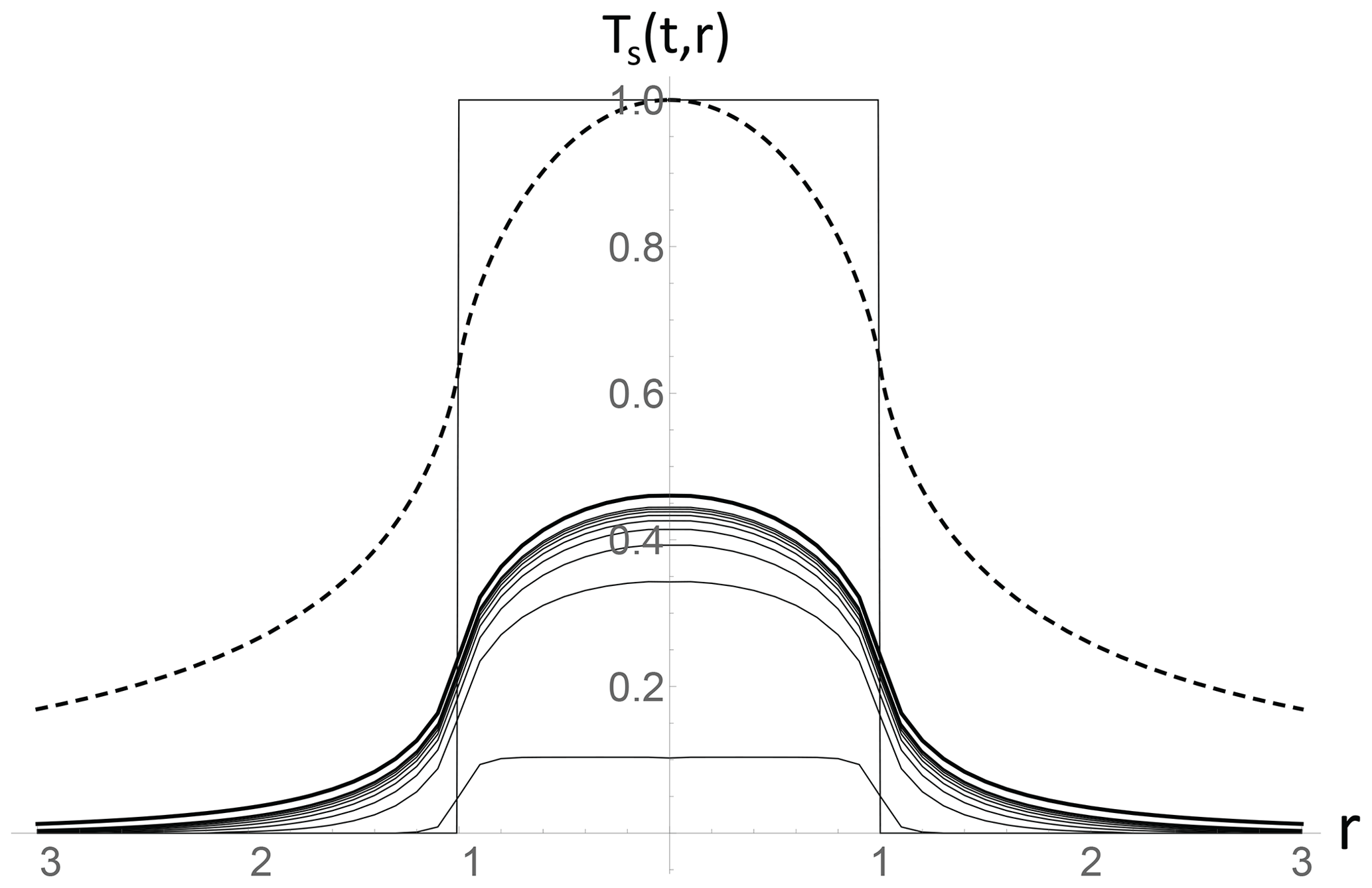
Figure 4 This is the step response in time and (circular) step in space for conductive–radiative forcing. Lines for t= 0.01 (bottom) and then for t= 0.2, 0.4, … 1.6 (black, bottom to top; the thick black line is for t=∞ or equilibrium). The nondimensional forcing is the rectangle (from unit circular forcing). Also shown (top dashed) is the equilibrium when the forcing is purely due to unit conductive heating over the unit circle.

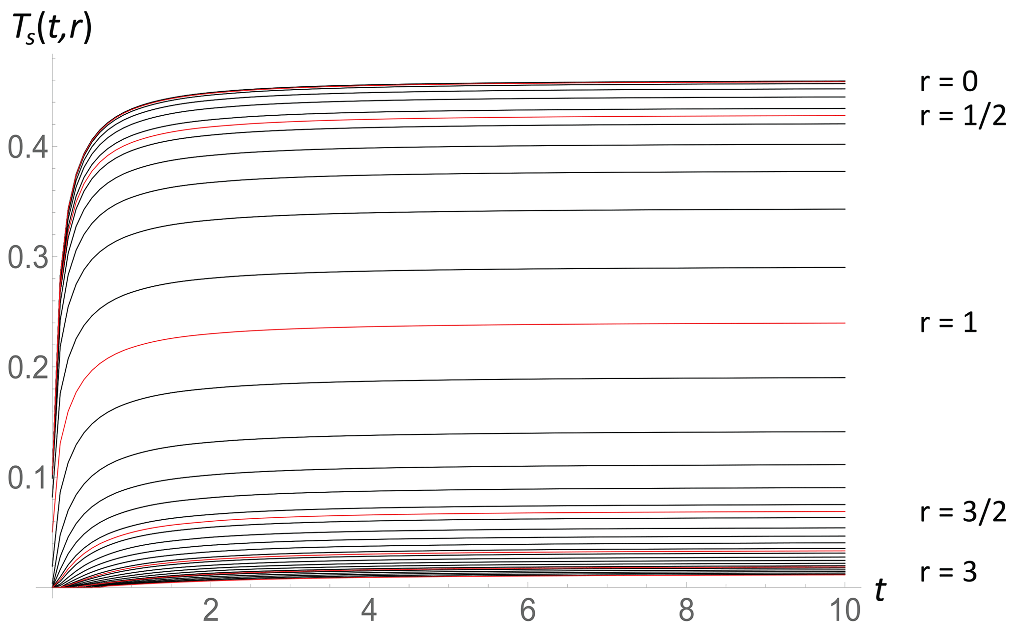
Figure 5 The response to a unit intensity forcing in the unit circle. The temperature as a function of nondimensional time is given for different distances from the center: top (r= 0) to bottom (r= 3) from the same data as before: red every $\mathrm{1}/\mathrm{2}$ and black every 0.1 (top r= 0; bottom r= 3).

Figure 6 Space–time contours for unit circle forcing as a function of nondimensional time (left to right) and nondimensional horizontal distance (vertical axis).

Figures 5 and 6 show the same evolution but with temperature as a function of time for various distances (Fig. 5) and as contours in space–time (Fig. 6). We see that equilibrium is largely established in the first two relaxation times (here τ= 1), and most of the perturbation is confined to two horizontal diffusion distances (here, l_h= 1).

2.3 Comparison of the HEBE with the standard 1D Budyko–Sellers model on a sphere

It is helpful to clearly understand the similarities and differences between the HEBE and the usual 1D (latitudinal) Budyko–Sellers (B–S) approach (see the comprehensive monograph in North and Kim, 2017; see Zhuang et al., 2017, and Ziegler and Rehfeld, 2020, for recent applications and development). Since the B–S model is on a sphere but with only latitudinal dependence, write the horizontal transport term ∇_h⋅D_B-S∇_h using gradient and divergence operators as ${\mathrm{\nabla }}_{\mathrm{h}}\cdot =-\frac{\mathrm{1}}{R}\frac{\mathrm{d}}{\mathrm{d}\mathit{\mu }}\sqrt{\mathrm{1}-{\mathit{\mu }}^{\mathrm{2}}}$ and ${\mathrm{\nabla }}_{\mathrm{h}}=-\frac{\sqrt{\mathrm{1}-{\mathit{\mu }}^{\mathrm{2}}}}{R}\frac{\mathrm{d}}{\mathrm{d}\mathit{\mu }}$, with μ= cos θ, θ= colatitude, and R the radius of the Earth. In standard notation (North and Kim, 2017) the B–S equation is thus written as

$$\begin{array}{}\text{(26)}& \begin{array}{rl}C{\displaystyle \frac{\partial T}{\partial t}}& -{\displaystyle \frac{\partial }{\partial \mathit{\mu }}}\left(D_{\text{B-S}}\left(\mathit{\mu }\right)\left(\mathrm{1}-{\mathit{\mu }}^{\mathrm{2}}\right){\displaystyle \frac{\partial }{\partial \mathit{\mu }}}T\right)+B\left(\mathit{\mu }\right)T\\ & +A\left(\mathit{\mu }\right)=Q_{\mathrm{0}}H\left(\mathit{\mu }\right);H\left(\mathit{\mu }\right)=S\left(\mathit{\mu }\right)a\left(\mathit{\mu }\right),\end{array}\end{array}$$

where C is the specific heat per area, D_B-S is the thermal conductivity per radian of arc, B is the climate feedback parameter, ($B=\mathrm{1}/s$) is the inverse of climate sensitivity, Q₀ is the solar constant, H is the heat function, S is the insolation distribution function, a is the co-albedo, and A is the constant term from the linearization of the black-body emission. If we measure temperatures with respect to the mean (reference) Earth temperature so that the A term balances the mean forcing, then the B–S equation with dimensionless operators can be written as

$$\begin{array}{}\text{(27)}& \left(\mathit{\tau }{\displaystyle \frac{\partial }{\partial t}}-s{\displaystyle \frac{\partial }{\partial \mathit{\mu }}}{D}_{\text{B-S}}\left(\mathit{\mu }\right)\left(\mathrm{1}-{\mathit{\mu }}^{\mathrm{2}}\right){\displaystyle \frac{\partial }{\partial \mathit{\mu }}}\right)T+T=sF\end{array}$$

(the product sD_B-S is dimensionless, $\mathit{\tau }=C/B$), where F is the anomaly with respect to the global average.

In Part 1 (Sect. 3.1.1), the horizontal transport operator was expressed in terms of the transport coefficient D_F that allows the HEBE to be written in the form

$$\begin{array}{}\text{(28)}& \begin{array}{rl}{\left(\mathit{\tau }{\displaystyle \frac{\partial }{\partial t}}+\mathit{\zeta }\right)}^{\mathrm{1}/\mathrm{2}}T& +T=sF;\mathit{\zeta }=-sR{\mathrm{\nabla }}_{\mathrm{h}}\cdot D_F{\mathrm{\nabla }}_{\mathrm{h}};\\ & D_F\left(\mathit{x}\right)={\displaystyle \frac{l_{\mathrm{h}}\left(\mathit{x}\right)}{Rs\left(\mathit{x}\right)}}={\mathit{\kappa }}_{\mathrm{h}}{\displaystyle \frac{\mathit{\beta }\mathit{\rho }c}{R}},\end{array}\end{array}$$

where $\mathit{\beta }={\left({\mathit{\kappa }}_{\mathrm{v}}/{\mathit{\kappa }}_{\mathrm{h}}\right)}^{\mathrm{1}/\mathrm{2}}$. Using $\mathit{\zeta }=-s\frac{d}{d\mathit{\mu }}{D}_F\left(\mathit{\mu }\right)\left(\mathrm{1}-{\mathit{\mu }}^{\mathrm{2}}\right)\frac{d}{d\mathit{\mu }}$ for the transport operator, we obtain the 1D HEBE on the sphere:

$$\begin{array}{}\text{(29)}& {\left(\mathit{\tau }{\displaystyle \frac{\partial }{\partial t}}-s{\displaystyle \frac{\partial }{\partial \mathit{\mu }}}{D}_F\left(\mathit{\mu }\right)\left(\mathrm{1}-{\mathit{\mu }}^{\mathrm{2}}\right){\displaystyle \frac{\partial }{\partial \mathit{\mu }}}\right)}^{\mathrm{1}/\mathrm{2}}T+T=sF.\end{array}$$

In the case of constant thermal diffusion coefficients we may solve both the B–S equation and the HEBE using Legendre polynomials P_n(μ) that are eigenfunctions of the Laplacian: $\left(-\frac{\partial }{\partial \mathit{\mu }}\left(\mathrm{1}-{\mathit{\mu }}^{\mathrm{2}}\right)\frac{\partial }{\partial \mathit{\mu }}\right)P_n\left(\mathit{\mu }\right)=n\left(n+\mathrm{1}\right)P_n\left(\mathit{\mu }\right)$ (with boundary conditions at the poles being zero horizontal heat flux; see also Appendix C for more general results on the sphere). Expanding the temperature and forcing in terms of the Legendre polynomials and taking Laplace transforms of the coefficients in time, we obtain the following.

$$\begin{array}{}\text{(30)}& \begin{array}{rl}& T\left(t,\mathit{\mu }\right)=\sum _{n=\mathrm{0}}^{\mathrm{\infty }}{T}_n\left(t\right)P_n\left(\mathit{\mu }\right)\stackrel{\mathrm{LT}}{\leftrightarrow }\widehat{T}\left(p,\mathit{\mu }\right)=\sum _{n=\mathrm{0}}^{\mathrm{\infty }}{\widehat{T}}_n\left(p\right)P_n\left(\mathit{\mu }\right)\\ & F\left(t,\mathit{\mu }\right)=\sum _{n=\mathrm{0}}^{\mathrm{\infty }}{F}_n\left(t\right)P_n\left(\mathit{\mu }\right)\stackrel{\mathrm{LT}}{\leftrightarrow }\widehat{F}\left(p,\mathit{\mu }\right)=\sum _{n=\mathrm{0}}^{\mathrm{\infty }}{\widehat{F}}_n\left(p\right)P_n\left(\mathit{\mu }\right)\end{array}\end{array}$$

We then obtain equations for the Laplace transform of the nth Legendre coefficients as

$$\begin{array}{}\text{(31)}& \begin{array}{rl}& \left(\mathit{\tau }p+{\mathit{\xi }}_{\text{B-S},n}\right)\widehat{T_n}+{\widehat{T}}_n=s{\widehat{F}}_n;{\mathit{\xi }}_{\text{B-S},n}=s{D}_{\text{B-S}}n\left(n+\mathrm{1}\right)\\ & {\left(\mathit{\tau }p+{\mathit{\xi }}_{F,n}\right)}^{\mathrm{1}/\mathrm{2}}{\widehat{T}}_n+{\widehat{T}}_n=s{\widehat{F}}_n;{\mathit{\xi }}_{F,n}=s{D}_{F}n\left(n+\mathrm{1}\right),\end{array}\end{array}$$

so that

$$\begin{array}{}\text{(32)}& \begin{array}{rl}{\widehat{T}}_n\left(p\right)=& s{\widehat{G}}_{\mathit{\delta }}^{\left(n\right)}\left(p\right){\widehat{F}}_n\left(p\right);\\ & {\widehat{G}}_{\mathit{\delta },\text{B-S}}^{\left(n\right)}\left(p\right)={\widehat{G}}_{\mathit{\delta },h=\mathrm{1}}\left(\mathit{\tau }p+{\mathit{\xi }}_{\text{B-S},n}\right);\\ & {\widehat{G}}_{\mathit{\delta },F}^{\left(n\right)}\left(p\right)={\widehat{G}}_{\mathit{\delta },h=\mathrm{1}/\mathrm{2}}\left(\mathit{\tau }p+{\mathit{\xi }}_{F,n}\right);\\ & {\widehat{G}}_{\mathit{\delta },h}\left(p\right)={\displaystyle \frac{\mathrm{1}}{\mathrm{1}+p^h}}.\end{array}\end{array}$$

In real space,

$$\begin{array}{}\text{(33)}& \begin{array}{rl}& {\mathit{\tau }}^{-\mathrm{1}}{e}^{-{\mathit{\xi }}_{\text{B-S},n}t/\mathit{\tau }}{G}_{\mathit{\delta },\text{B-S}}^{\left(n\right)}\left(t/\mathit{\tau }\right)\stackrel{\mathrm{LT}}{\leftrightarrow }{\widehat{G}}_{\mathit{\delta },\mathrm{1}}^{\left(n\right)}\left(p\mathit{\tau }+{\mathit{\xi }}_{\text{B-S},n}\right)\\ & {\mathit{\tau }}^{-\mathrm{1}}{e}^{-{\mathit{\xi }}_{\mathrm{1}/\mathrm{2},n}t/\mathit{\tau }}{G}_{\mathit{\delta },F}^{\left(n\right)}\left(t/\mathit{\tau }\right)\stackrel{\mathrm{LT}}{\leftrightarrow }{\widehat{G}}_{\mathit{\delta },\mathrm{1}/\mathrm{2}}^{\left(n\right)}\left(p\mathit{\tau }+{\mathit{\xi }}_{F,n}\right).\end{array}\end{array}$$

Note that the generalization to the FEBE is obtained by the replacement τp→(τp)^2h so that ${\widehat{G}}_{\mathit{\delta },h}^{\left(n\right)}\left(p\right)={\left(\mathrm{1}+{\left({\left(\mathit{\tau }p\right)}^{\mathrm{2}h}+{\mathit{\xi }}_{F,n}\right)}^{\mathrm{1}/\mathrm{2}}\right)}^{-\mathrm{1}}$, whereas ${\widehat{G}}_{\mathit{\delta },B-S}^{\left(n\right)}\left(p\right)={\left(\mathrm{1}+\mathit{\tau }p+{\mathit{\xi }}_{\text{B-S},n}\right)}^{-\mathrm{1}}$ so that ${\widehat{G}}_{\mathit{\delta },\text{B-S}}^{\left(n\right)}$ (and hence the B–S model) is not a special case of the FEBE. Using

$$\begin{array}{}\text{(34)}& \begin{array}{rl}& e^{-t}\stackrel{\mathrm{LT}}{\leftrightarrow }{\displaystyle \frac{\mathrm{1}}{\mathrm{1}+p}}\\ & \sqrt{{\displaystyle \frac{\mathrm{1}}{\mathit{\pi }t}}}-e^{t/\mathit{\tau }}\mathrm{erf}c\sqrt{t}\stackrel{\mathrm{LT}}{\leftrightarrow }{\displaystyle \frac{\mathrm{1}}{\mathrm{1}+p^{\mathrm{1}/\mathrm{2}}}}\end{array}\end{array}$$

(Eq. 35, Part 1) and combining this with Eq. (33), we obtain the following for the impulse responses.

$$\begin{array}{}\text{(35)}& \begin{array}{rl}& G_{\mathit{\delta },\text{B-S}}^{\left(n\right)}\left(t\right)={\mathit{\tau }}^{-\mathrm{1}}{e}^{-\left(\mathrm{1}+{\mathit{\xi }}_{\text{B-S},n}\right)t/\mathit{\tau }}\\ & G_{\mathit{\delta },F}^{\left(n\right)}\left(t\right)={\mathit{\tau }}^{-\mathrm{1}}{e}^{-{\mathit{\xi }}_{F,n}t/\mathit{\tau }}\left(\sqrt{{\displaystyle \frac{\mathit{\tau }}{\mathit{\pi }t}}}-e^{t/\mathit{\tau }}\mathrm{erfc}\sqrt{{\displaystyle \frac{t}{\mathit{\tau }}}}\right)\end{array}\end{array}$$

Integrating these with respect to t, we obtain the step responses as follows.

$$\begin{array}{}\text{(36)}& \begin{array}{rl}& G_{\mathrm{\Theta },\text{B-S}}^{\left(n\right)}\left(t\right)={\displaystyle \frac{\mathrm{1}}{{\mathit{\xi }}_{\text{B-S},n}+\mathrm{1}}}\left(\mathrm{1}-e^{-\left({\mathit{\xi }}_{\text{B-S},n}+\mathrm{1}\right)t/\mathit{\tau }}\right)\\ & G_{\mathrm{\Theta },F}^{\left(n\right)}\left(t\right)={\displaystyle \frac{\sqrt{{\mathit{\xi }}_{F,n}}\mathrm{erf}\sqrt{{\mathit{\xi }}_{F,n}\frac{t}{\mathit{\tau }}}-\mathrm{1}+e^{-t\left({\mathit{\xi }}_{{}_{F,n}}-\mathrm{1}\right)/\mathit{\tau }}\mathrm{erfc}\sqrt{\frac{t}{\mathit{\tau }}}}{{\mathit{\xi }}_{F,n}-\mathrm{1}}}\end{array}\end{array}$$

The long-time limit represents Earth's energy balance (equilibrium).

$$\begin{array}{}\text{(37)}& \begin{array}{rl}& G_{\text{eq,B-S}}^{\left(n\right)}=G_{\mathrm{\Theta },\mathrm{1}}^{\left(n\right)}\left(\mathrm{\infty }\right)={\displaystyle \frac{\mathrm{1}}{\mathrm{1}+{\mathit{\xi }}_{\text{B-S},n}}}={\displaystyle \frac{\mathrm{1}}{\mathrm{1}+s{D}_{\text{B-S}}n\left(n+\mathrm{1}\right)}};\\ & G_{\mathrm{eq},\mathrm{F}}^{\left(n\right)}=G_{\mathrm{\Theta },F}^{\left(n\right)}\left(\mathrm{\infty }\right)={\displaystyle \frac{\mathrm{1}}{\mathrm{1}+\sqrt{{\mathit{\xi }}_{{}_{F,n}}}}}={\displaystyle \frac{\mathrm{1}}{\mathrm{1}+\sqrt{s{D}_{F}n\left(n+\mathrm{1}\right)}}}\\ & \mathit{\xi }\ge \mathrm{0}.\end{array}\end{array}$$

If ξ < 0, then there is an unphysical divergence so that sD_F must be > 0. Since P_n(μ) has n zeroes, n plays the role of wavenumber; it specifies structures of horizontal size $\approx \mathit{\pi }R/n$. Therefore, we see that the B–S model (where $G_{\mathrm{eq},\mathrm{B}-\mathrm{S}}$ falls off as n⁻²) will yield a much smoother equilibrium temperature distribution than the HEBE wherein it falls off as n⁻¹. Note that when generalized from the HEBE to the FEBE (with p→p^2h), this equilibrium result is unchanged.

For the HEBE, the short- and long-time behaviors are as follows.

$$G_{\mathrm{\Theta },F}^{\left(n\right)}\left(t\right)={\displaystyle \frac{\mathrm{2}{t}^{\mathrm{1}/\mathrm{2}}}{\sqrt{\mathit{\pi }\mathit{\tau }}}}-{\displaystyle \frac{t}{\mathit{\tau }}}-{\displaystyle \frac{\mathrm{2}\left({\mathit{\xi }}_{F,n}-\mathrm{2}\right)}{\mathrm{3}\sqrt{\mathit{\pi }}}}{\left({\displaystyle \frac{t}{\mathit{\tau }}}\right)}^{\mathrm{3}/\mathrm{2}}$$

$$+{\displaystyle \frac{\mathrm{1}}{\mathrm{2}}}\left({\mathit{\xi }}_{F,n}-\mathrm{1}\right){\left({\displaystyle \frac{t}{\mathit{\tau }}}\right)}^{\mathrm{2}}+\mathrm{\dots };t\ll \mathit{\tau };n\ge \mathrm{0}$$

$$G_{\mathrm{\Theta },F}^{\left(\mathrm{0}\right)}\left(t\right)=\mathrm{1}-{\displaystyle \frac{\mathrm{1}}{\sqrt{\mathit{\pi }t}}}+{\displaystyle \frac{\mathrm{1}}{\mathrm{2}t\sqrt{\mathit{\pi }t}}}-\mathrm{\dots };t\gg \mathit{\tau };n=\mathrm{0}$$

$$G_{\mathrm{\Theta },F}^{\left(n\right)}\left(t\right)={\displaystyle \frac{\mathrm{1}}{\mathrm{1}+\sqrt{{\mathit{\xi }}_{F,n}}}}-{\displaystyle \frac{e^{-{\mathit{\xi }}_{F,n}t/\mathit{\tau }}}{\mathrm{2}\sqrt{\mathit{\pi }}{\mathit{\xi }}_{F,n}}}{\left({\displaystyle \frac{t}{\mathit{\tau }}}\right)}^{-\mathrm{3}/\mathrm{2}}$$

$$\begin{array}{}\text{(38)}& \times \left(\mathrm{1}-{\displaystyle \frac{\mathrm{3}}{\mathrm{2}}}\left({\displaystyle \frac{\mathrm{1}+{\mathit{\xi }}_{F,n}}{{\mathit{\xi }}_{F,n}t/\mathit{\tau }}}\right)+\mathrm{\dots }\right);t\gg \mathit{\tau };n\ge \mathrm{1}\end{array}$$

The asymptotic response for $G_{\mathrm{\Theta },F}^{\left(n\right)}\left(t\right)$ is interesting because it shows how quickly equilibrium is reached. When n= 0 we have P₀(μ)= 1 so that this component corresponds to the mean. Since ${\mathit{\xi }}_{F,\mathrm{0}}=\mathrm{0}$ we see that it is identical to the zero-dimensional result in Part 1: equilibrium is approached in a power-law fashion ($t^{-\mathrm{1}/\mathrm{2}}$ for large t), whereas for n= 0, the B–S model approach to equilibrium is exponential. However, for n≥ 1, HEBE power-law terms are exponentially damped with exponential decay time ${\mathit{\tau }}_{F,n}=\mathit{\tau }/{\mathit{\xi }}_{F,n}$, whereas the B–S model is exponentially damped for all n with ${\mathit{\tau }}_{\text{B-S},n}=\mathit{\tau }/\left(\mathrm{1}+{\mathit{\xi }}_{\text{B-S},n}\right)$.

In order to make a more detailed comparison between the models, we can follow North and Kim (2017), who consider a model with constant D_S-B that is north–south symmetric so that the odd-numbered polynomials vanish. They empirically give the climate equilibrium values for n= 0, 2, 4; the (constant) n= 0 term is used to obtain the mean temperature of 288 K. Other pertinent empirical data are s= $\mathrm{1}/B=$ 0.50 KW⁻¹ m², F₂= −180.7 W/m², F₄= 20.8 W m⁻², T₂= −30 K, and T₄= −4 K. From Eq. (37) for the equilibrium temperature Green's function, we obtain $T_{\mathrm{eq},\mathrm{n}}=s{G}_{\text{eq,B-S}}^{\left(n\right)}{F}_n$. The n= 2 relationship is used to estimate $D_{\text{B-S}}=\frac{\mathrm{1}}{\mathrm{6}s}\left(\frac{s{F}_{\mathrm{2}}}{T_{\mathrm{2}}}-\mathrm{1}\right)=$ 0.67 Wm⁻² K⁻¹. With this estimate, we obtain $T_{\mathrm{4}}=s{F}_{\mathrm{4}}/\left(\mathrm{1}+{\mathit{\xi }}_{\text{B-S},n}\right)=s{F}_{\mathrm{4}}/\left(\mathrm{1}+\mathrm{20}{D}_{\text{B-S}}s\right)\approx$ 1.35 K, which is not far from the empirical estimate T₄= −4 K (North and Kim, 2017), and it also yields the dimensionless quantity sD_B-S= 0.33. If we follow the same procedure for the HEBE, we estimate $D_F=\frac{\mathrm{1}}{\mathrm{6}s}{\left(\frac{s{F}_{\mathrm{2}}}{T_{\mathrm{2}}}-\mathrm{1}\right)}^{\mathrm{2}}$. Comparing this with the B–S relation, we find sD_F= 6 (sD_S−B)², the dimensionless sD_F= 0.67; hence D_F= 1.33 Wm⁻² K⁻¹, and T₄= 2.23 K (again not far from the data). We note that the ratio $D_F/D_{\text{B-S}}\approx$ 2 so that the estimates are close.

This information can be used to estimate l_h in the HEBE. From the definition of D_B-S as a thermal conduction coefficient per radian, we obtain $D_{\text{B-S}}=K/R$ so that ${\mathit{\kappa }}_{\mathrm{h}}=K/\mathit{\rho }c=R{D}_{\text{B-S}}/\mathit{\rho }c\approx \mathrm{1}$ m²/s (where K is the usual thermal conductivity). To find the transport length, we can use l_h=βκ_hρcs and $\mathit{\beta }={\left(\frac{{\mathit{\kappa }}_{\mathrm{v}}}{{\mathit{\kappa }}_{\mathrm{h}}}\right)}^{\mathrm{1}/\mathrm{2}}$ to obtain

$$\begin{array}{}\text{(39)}& {\displaystyle \frac{l_{\mathrm{h}}}{R}}=\mathit{\beta }s{D}_{\text{B-S}}.\end{array}$$

Alternatively, we can estimate l_h from the global-scale D_F:

$$\begin{array}{}\text{(40)}& {\displaystyle \frac{l_{\mathrm{h}}}{R}}=s{D}_F.\end{array}$$

We see that these l_h estimates differ by a factor of $\mathit{\beta }{D}_{\text{B-S}}/D_F\approx \mathit{\beta }/\mathrm{2}$. Since typical numerical models with resolutions of hundreds of kilometers use κ_v≈ 10⁻⁴ m²/s and κ_h≈ 1 m²/s, at least at these scales, β≈ 10⁻² so that the difference in the estimates may be large. For example, since sD_B-S≈ 0.33, we find that the former Eq. (39) yields l_h≈ 20 km, while the latter Eq. (40) yields l_h≈ 4000 km. One way to reconcile the difference is to assume that both κ_h and κ_v are highly variable in space. In this case, the ratio β that characterizes the horizontal–vertical effective diffusivity anisotropy will have a systematic scale dependence due to a difference in the scaling properties of κ_h and κ_v. Therefore, at global scales we may have β≈ 1 but at kilometric scales β≈ 10⁻². This may arise as a consequence of the scaling anisotropic horizontal structure of the atmosphere at weather scales, notably of the horizontal wind field in the 23/9D model (Schertzer and Lovejoy, 1985).

A different (possibly additional) way of reconciling the estimates is to consider the potentially large (multifractal) intermittency of the diffusivities that introduces a strong scale effect. For example, Havlin and Ben-Avraham (1987), Weissman (1988), and Lovejoy et al. (1998) show that in 1D, the large-scale effective thermal resistance ρ – the inverse diffusivity – is the average of the small-scale resistances. If we denote the spatial averages over a scale L by a subscript and assume that the resistivity is scaling (scale-invariant) up to planetary scales (denote this by R), then it will generally follow the following multifractal statistics:

$$\begin{array}{}\text{(41)}& 〈{\mathit{\rho }}_L^q〉={\left({\displaystyle \frac{R}{L}}\right)}^{K_{\mathit{\rho }}\left(q\right)}〈{\mathit{\rho }}_R^q〉,\end{array}$$

where the angle brackets denote statistical averages and K_ρ(q) is the moment scaling function that characterizes the scaling of the qth-order statistical moment order of the thermal resistance (not to be confused with the thermal conductivity).

The thermal resistance is proportional to the inverse thermal diffusivity; therefore, the effective HEBE diffusive transport coefficient at scale L satisfies

$$\begin{array}{}\text{(42)}& D_{F,L}\propto {\mathit{\kappa }}_{h,L}\propto {\left({\mathit{\rho }}^{-\mathrm{1}}\right)}_L\approx {\left({\displaystyle \frac{R}{L}}\right)}^{-K_{\mathit{\rho }}\left(-\mathrm{1}\right)}{D}_{F,R},\end{array}$$

where ${\left({\mathit{\rho }}^{-\mathrm{1}}\right)}_L$ is the average of $\mathrm{1}/\mathit{\rho }$ over horizontal scale L. Finally, using $l_{\mathrm{h},L}\propto D_{F,L}$, we obtain

$$\begin{array}{}\text{(43)}& l_{\mathrm{h},L}\propto {\left({\displaystyle \frac{L}{R}}\right)}^{K_{\mathit{\rho }}\left(-\mathrm{1}\right)}{l}_{\mathrm{h},R},\end{array}$$

which relates the average transport length at small scales L and planetary scales R. Depending on K_ρ(−1), the ratio $l_{\mathrm{h},L}/l_{\mathrm{h},R}$ can be quite small. For example, if the thermal resistivity statistics are taken as lognormal, then $K_{\mathit{\rho }}\left(q\right)=C_{\mathrm{1}}q\left(q-\mathrm{1}\right)$ so that $K_{\mathit{\rho }}\left(-\mathrm{1}\right)=\mathrm{2}{C}_{\mathrm{1}}$ and $l_{\mathrm{h},L}\propto {\left(L/R\right)}^{\mathrm{2}{C}_{\mathrm{1}}}{l}_{\mathrm{h},R}$. As discussed in Appendix A, C₁≈ 0.16 for the temperature in space (see also Lovejoy, 2018). Using this value as a guide, we find $l_{\mathrm{h},L}\propto {\left(L/R\right)}^{\mathrm{0.32}}{l}_{\mathrm{h},R}$ so that, depending on the small-scale resolution L, such spatial variability of the diffusivity can easily explain a factor of 10 or more increase in the effective transport length at large scales. Clearly the scale dependence of κ_h and κ_v is an important topic for future FEBE research.

3 The inhomogeneous heat equation

3.1 Babenko's method

The homogeneous heat equation in a semi-infinite domain is a classical problem, and conductive–radiative surface boundary conditions naturally lead to fractional-order operators: the HEBE and GHEBE. Although we have seen that fractional operators appear quite naturally, their advantages are much more compelling for the more realistic inhomogeneous equations relevant for the Earth. I therefore proceed to derive the inhomogeneous HEBE and GHEBE using Babenko's method. The more usual application is to find the surface heat flux given a solution to the conduction equation (see, for example, Magin et al., 2004; Chenkuan and Clarkson, 2018), although the following application appears to be original. In the inhomogeneous case with τ=τ(x), l_h=l_h(x), l_v= l_v(x), and α=α(x), there is no unique nondimensionalization. Therefore, I express the inhomogeneous anomaly heat equation with nondimensional operators as

$$\begin{array}{}\text{(44)}& \left(\mathit{\tau }{\displaystyle \frac{\partial }{\partial t}}+l_{\mathrm{h}}\mathit{\zeta }-{\left(l_{\mathrm{v}}{\displaystyle \frac{\partial }{\partial z}}\right)}^{\mathrm{2}}\right)T=\mathrm{0};\mathit{\zeta }=\left(\mathit{\alpha }\cdot {\mathrm{\nabla }}_{\mathrm{h}}+l_{\mathrm{h}}\left(-{\mathrm{\nabla }}_{\mathrm{h}}^{\mathrm{2}}\right)\right),\end{array}$$

where I have used ${\mathit{\kappa }}_{\mathrm{v}}\left(\mathit{x}\right)=l_{\mathrm{v}}^{\mathrm{2}}$ and $\frac{{\partial }^{\mathrm{2}}}{\partial z^{\mathrm{2}}}={\left(l_{\mathrm{v}}\frac{\partial }{\partial z}\right)}^{\mathrm{2}}$ and ζ is a time-independent horizontal transport operator allowing for both advective and diffusive transport. Under fairly general conditions, when ζ operates on the temperature field, it is proportional to the nondimensional divergence of the horizontal heat flux (discussed in Part 1; see Eq. 4). Since the forcing is via the surface boundary condition rather than by an inhomogeneous term, Eq. (44) is mathematically homogeneous.

The first step in Babenko's method (see, e.g., Podlubny, 1999; Magin et al., 2004) is to factor the differential operator as follows.

$$\begin{array}{}\text{(45)}& \left(\mathrm{\Lambda }+l_{\mathrm{v}}{\displaystyle \frac{\partial }{\partial z}}\right)\left(\mathrm{\Lambda }-l_{\mathrm{v}}{\displaystyle \frac{\partial }{\partial z}}\right)T=\mathrm{0};\mathrm{\Lambda }={\left(\mathit{\tau }{\displaystyle \frac{\partial }{\partial t}}+l_{\mathrm{h}}\mathit{\zeta }\right)}^{\mathrm{1}/\mathrm{2}}\end{array}$$

As usual, the general solution of a homogeneous equation is a linear combination of elementary solutions A₊ and A₋.

$$\begin{array}{}\text{(46)}& \left(\mathrm{\Lambda }+l_{\mathrm{v}}{\displaystyle \frac{\partial }{\partial z}}\right)A_{+}\left(t,\mathit{x};z\right)=\mathrm{0};\left(\mathrm{\Lambda }-l_{\mathrm{v}}{\displaystyle \frac{\partial }{\partial z}}\right)A_{-}\left(t,\mathit{x};z\right)=\mathrm{0}\end{array}$$

The A₊ solution leads to solutions that diverge at $z=-\mathrm{\infty }$, whereas A₋ leads to the required physical solutions with $T\left(-\mathrm{\infty }\right)=\mathrm{0}$ (Podlubny, 1999). Therefore, we are interested in solutions to

$$\begin{array}{}\text{(47)}& \left(\mathrm{\Lambda }-l_{\mathrm{v}}{\displaystyle \frac{\partial }{\partial z}}\right)T\left(t,\mathit{x};z\right)=\mathrm{0}.\end{array}$$

Putting z= 0 and using $Q_z=-\left(l_{\mathrm{v}}/s\right)\partial T/\partial z$ (Part 1, Eq. 22), we obtain

$$\begin{array}{}\text{(48)}& \begin{array}{rl}{\left(\mathit{\tau }{\displaystyle \frac{\partial }{\partial t}}+l_{\mathrm{h}}\mathit{\zeta }\right)}^{\mathrm{1}/\mathrm{2}}& T_{\mathrm{s}}=l_{\mathrm{v}}{\left.{\displaystyle \frac{\partial T}{\partial z}}\right|}_{z=\mathrm{0}}=s{Q}_s;\\ & \begin{array}{l}{T}_{\mathrm{s}}\left(t,\mathit{x}\right)=T\left(t,\mathit{x};\mathrm{0}\right)\\ Q_{\mathrm{s}}\left(t,\mathit{x}\right)=-{\left({\mathit{Q}}_{\mathrm{d}}\left(t,\mathit{x};\mathrm{0}\right)\right)}_z,\end{array}\end{array}\end{array}$$

where T_s(t,x) is the surface temperature anomaly and Q_s is the heat flux into the surface (the negative of $Q_{\mathrm{s},\mathrm{d},z}$, which is the z component of the surface conductive – sensible – heat flux). Before interpreting the half-order operator on the left, we can already give this equation a physical interpretation. When Q_s > 0, sensible heat is forced into the Earth. Some of it is stored in the subsurface (the $\mathit{\tau }\frac{\partial }{\partial t}$ term with the same horizontal position x but stored by heating up the subsurface, z < 0), and some of the heat (the l_hζ term) is the contribution from the horizontal divergence of the heat flux to the storage (and conversely when Q_s < 0). We can also understand the basic difference between the A₊ and A₋ solutions: whereas the physically relevant A₋ solution corresponds to energy storage and horizontal transport in the region z < 0, the A₊ solutions correspond to the region z > 0 assumed to be devoid of conducting material.

The final step is to use the fact that the conductive heat flux Q_s is equal to the radiative imbalance (Part 1, Fig. 1).

$$\begin{array}{}\text{(49)}& Q_{\mathrm{s}}=R_{\downarrow }-R_{\uparrow }=-{\displaystyle \frac{T_{\mathrm{s}}}{s}}-F\end{array}$$

Combining Eqs. (48) and (49), we obtain the inhomogeneous generalized half-order energy balance equation (GHEBE).

$$\begin{array}{}\text{(50)}& \begin{array}{rl}{\left(\mathit{\tau }\left(\mathit{x}\right){\displaystyle \frac{\partial }{\partial t}}+l_{\mathrm{h}}\left(\mathit{x}\right)\mathit{\zeta }\left(\mathit{x}\right)\right)}^{\mathrm{1}/\mathrm{2}}& T_{\mathrm{s}}\left(t,\mathit{x}\right)+T_{\mathrm{s}}\left(t,\mathit{x}\right)\\ & =s\left(\mathit{x}\right)F\left(t,\mathit{x}\right)\end{array}\end{array}$$

If needed, the internal field $T(t,\mathit{x};z)$ can be found by solving Eq. (50) for T_s(t,x), which is the z= 0 boundary condition for the full Eq. (44). We see that Eq. (50) reduces to the homogeneous GHEBE (Eq. 17) when τ, l_h, s, and α are constant.

By comparing this derivation with that of the homogeneous GHEBE via the classical Laplace–Fourier transform method (Sect. 2.1), it is clear that Babenko's method is very similar but is more general. Whereas in the homogeneous equation, the transforms reduce the derivative operations to algebra, the difficulty with Babenko's method is to find proper interpretations of the fractional operators. However, in the above, I assumed that τ was only a function of position so that Laplace (or Fourier) transform methods still apply in the time domain. In the next section I discuss the more challenging interpretation of the fractional inhomogeneous spatial operators.

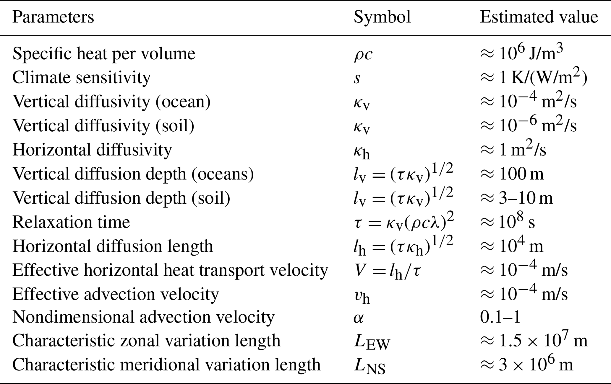
Table 1 Empirical estimates of the parameters used in this paper; see Appendix A for details.

3.2 The zeroth-order high-frequency GHEBE: the HEBE

Before discussing the inhomogeneous GHEBE, consider the case in which the horizontal term l_hζ is small compared to $\mathit{\tau }\frac{\partial }{\partial t}$; below we argue that this is a good approximation for scales up to years and decades as well as greater than tens of kilometers (Table 1, Appendix A). Recall that the horizontal transport term is in fact proportional to the divergence of the horizontal heat flux so that it may be small even when heat fluxes are significant (Trenberth et al., 2009). Alternatively, in globally averaged models, there are no horizontal inhomogeneities so that ζ= 0. In these cases $\mathrm{\Lambda }=\mathit{\tau }{\left(\mathit{x}\right)}^{\mathrm{1}/\mathrm{2}}\frac{{\partial }^{\mathrm{1}/\mathrm{2}}}{\partial t^{\mathrm{1}/\mathrm{2}}}$, and we obtain the inhomogeneous HEBE as a special $h=\mathrm{1}/\mathrm{2}$ case of the inhomogeneous FEBE:

$$\begin{array}{}\text{(51)}& \mathit{\tau }{\left(\mathit{x}\right)}_{-\mathrm{\infty }}^h{D}_t^h{T}_{\mathrm{s}}\left(t,\mathit{x}\right)+T_{\mathrm{s}}(t,\mathit{x})=s\left(\mathit{x}\right)F(t,\mathit{x}).\end{array}$$

I have written it with a general h since, as in Part 1, an inhomogeneous version of the EBE may be obtained with h= 1. I have also used the Weyl derivative (i.e., from $t=-\mathrm{\infty })$ since this accommodated periodic or statistically stationary forcing as well as forcing starting at t= 0 (in this case we simply consider F= 0 for t≤ 0). Equation (50) shows that the HEBE only depends on the local climate sensitivity and the local relaxation time. We will see below that explicit dependence on the horizontal transport (v, κ_h) and specific heat per volume ρc is only important at scales somewhat smaller than the transport length scale (or alternatively at extremely long timescales; Sect. 3.6). Before solving the HEBE, it is instructive to introduce the notation $T_{\mathrm{\infty }}\left(t,\mathit{x}\right)=s\left(\mathit{x}\right)F(t,\mathit{x})$. T_∞ is the equilibrium temperature that would be reached if at time t at each location x for longer times, F was suddenly fixed at that value. With this notation, we may integrate both sides of Eq. (51) by order h and multiply by τ^−h to obtain the following.

$$\begin{array}{}\text{(52)}& \begin{array}{rl}{T}_{\mathrm{s}}\left(t,\mathit{x}\right)=& {\displaystyle \frac{\mathrm{1}}{\mathrm{\Gamma }\left(h\right)}}\underset{-\mathrm{\infty }}{\overset{t}{\int }}{\left({\displaystyle \frac{t-u}{\mathit{\tau }\left(\mathit{x}\right)}}\right)}^{h-\mathrm{1}}\left(T_{\mathrm{\infty }}\left(u,\mathit{x}\right)-T_{\mathrm{s}}\left(u,\mathit{x}\right)\right){\displaystyle \frac{\mathrm{d}u}{\mathit{\tau }\left(\mathit{x}\right)}};\\ & \mathrm{0}<h<\mathrm{1}\end{array}\end{array}$$

Written in this form, it is obvious that the temperature is constantly relaxing in a power-law manner to T_∞ (although if F is time-dependent, equilibrium will in general never in fact be established). In the usual EBM special case (h= 1), the power law must be replaced by an exponential, and the HEBE is obtained with h= 1/2. Since T_∞=sF, the deviation from T_∞ (the term ${\mathit{\tau }}_{-\mathrm{\infty }}^h{D}_t^h{T}_{\mathrm{s}}$ in Eq. 51) physically corresponds to the energy imbalance, and as before, it is a power-law long-memory energy storage term.

The FEBE is a linear differential equation that can be solved using Green's functions (Miller and Ross, 1993; Podlubny, 1999). The solution is

$$\begin{array}{}\text{(53)}& T_{\mathrm{s}}\left(\mathit{x},t\right)={\displaystyle \frac{s\left(\mathit{x}\right)}{\mathit{\tau }\left(\mathit{x}\right)}}\underset{-\mathrm{\infty }}{\overset{t}{\int }}{G}_{\mathit{\delta },h}\left({\displaystyle \frac{t-u}{\mathit{\tau }\left(\mathit{x}\right)}}\right)F(\mathit{x},u)\mathrm{d}u,\end{array}$$

where G_δ,h is the h-order Mittag–Leffler impulse response Green's function (see e.g. Lovejoy, 2019a). In general, G_δ,h is only expressible in terms of infinite series; exceptions are the h= 1 EBE ($G_{\mathit{\delta },\mathrm{1}}=e^{-t})$ and the h= $\mathrm{1}/\mathrm{2}$ HEBE (Eq. 33).

The corresponding step response $G_{\mathrm{\Theta },\mathrm{1}/\mathrm{2}}$ is the integral of $G_{\mathit{\delta },\mathrm{1}/\mathrm{2}}$ (respectively $G_{\mathrm{1},\mathrm{1}/\mathrm{2}}$ and $G_{\mathrm{0},\mathrm{1}/\mathrm{2}}$ in the notation in Eq. 36, Part 1). It describes relaxation to equilibrium when F is a step function; similarly, the ramp (linear forcing, second integral of a δ function) response $G_{\mathrm{2},\mathrm{1}/\mathrm{2}}$ (Eq. 36, Part 1) is the integral of the step response.

3.3 Some features of stochastic forcing

The FEBE and the HEBE are examples of fractional relaxation equations; these have primarily been discussed in the context of deterministic forcings that start at t= 0. The corresponding stochastic fractional relaxation processes (in physics referred to as the fractional Langevin equations or FLEs; see the references in Lovejoy, 2019a) here correspond to stochastic internal forcing. The FLEs have received little attention, although Kobelev and Romanov (2000) and West et al. (2003) discuss the corresponding nonstationary random walks. The statistically stationary stochastic case that results when Weyl rather than Riemann–Liouville fractional derivatives are used is treated in Lovejoy (2019a), including the HEBE autocorrelation function and prediction problem (and its limits) when F is Gaussian white noise.

To understand the noise-driven HEBE, it is helpful to Fourier-analyze it using $\left({}_{-\mathrm{\infty }}{D}_t^h\right)\stackrel{\mathrm{Fourier}}{\to }{\left(i\mathit{\omega }\right)}^h$ (Lovejoy, 2019a; Sect. 3.3, Part 1). At high frequencies, the derivative (energy storage) term dominates so that the temperature is a fractional integral (order h) of the forcing. At low frequencies, the derivative term can be neglected so that T≈sF, implying that the equilibrium temperature follows the forcing and that s is indeed the usual climate sensitivity.

Alternatively, in real space, if F(t) is a unit step function Θ(t) and s= 1, then for h≠ 1 the long-time relaxation to the equilibrium temperature response is a power law: $G_{\mathrm{\Theta },h}\left(t\right)\approx \mathrm{1}-t^{-h}$ (Part 1, Eq. 33). Similarly, for small t and h < 1, the impulse response is singular: $G_{\mathit{\delta },h}\left(t\right)\approx t^{h-\mathrm{1}}$ (Part 1, Eq. 33). Due to this singularity, when F(t) is Gaussian white noise, at high frequencies, T will be fractional Gaussian noise (fGn) with the exponent $H=h-\mathrm{1}/\mathrm{2}$. Averages over time Δt will behave as ${〈T_{\mathrm{\Delta }t}^{\mathrm{2}}〉}^{\mathrm{1}/\mathrm{2}}\propto \mathrm{\Delta }{t}^H$ (H is the fluctuation exponent – for fGn, −1 < H < 0, and for its integral–fractional Brownian motion, fBm, the fluctuation exponent is H+1; to avoid confusion, note that the Hurst parameters H^′ of fGn and for the corresponding fBm are equal so that $H^{\prime }=H+\mathrm{1}$ and $H^{\prime }=H$, respectively). When $h\le \mathrm{1}/\mathrm{2}$ (H≤0) and the resolution is increased (Δt→0), this implies strong resolution dependencies (mathematically, small-scale divergences), so it is important in data analysis, including the estimation of the temperature of the Earth (Lovejoy, 2017). When forced by white noise, the HEBE is exactly at the critical value H= 0 so that its high frequency (up to the relaxation time) corresponds to $\mathrm{1}/f$ noise. A particularly relevant aspect is that the correlation function and spectrum change very slowly from high to low frequencies (Lovejoy, 2019a). With data over a limited ranges of scales – e.g., months to decades – depending on the relaxation time τ, the HEBE could mimic the FEBE with any h in the range $\mathrm{0}\mathit{<}h\le \mathrm{1}/\mathrm{2}$ (hence, $-\mathrm{1}/\mathrm{2}\le H\le \mathrm{0}$). It is thus possible that geographical variations in H reported in Lovejoy et al. (2017) are spurious consequences of geographical variations in τ(x).

At global scales, the high- and low-frequency HEBE behaviors are close to observations. For example, the global value h=  0.5±0.2 was found for the long-time behavior needed to project the Earth's temperature to 2100. Hebert (2017), Hébert et al. (2021), and Procyk et al. (2020), also using centennial-scale global temperature estimates but using the FEBE directly, found the less uncertain h=  0.38±0.05. Using data at monthly and seasonal scales, Del Rio Amador and Lovejoy (2019) found and used the value h= 0.42 ± 0.03. Appendix B discusses the spatial cross-correlation matrix implied by the HEBE that is needed, for example, in calculating empirical orthogonal functions (EOFs) or for the space–time macroweather model developed in Del Rio Amador and Lovejoy (2021b).

Although the HEBE was derived for anomalies, these were not defined as small perturbations but rather as time-varying components of the full solution of the temperature (energy) equation with the time-independent part corresponding to the climate state. The only point at which T was assumed to be small was with respect to the absolute local climate temperature about which the black-body radiation was linearized, a fairly weak restriction on T. I could also mention that by allowing the albedo or other parameters to change in time, the HEBE could easily be extended to the study of past or future climates for which it would broaden the spectrum, potentially improving the modeling of glacial cycles.

An important feature of fractional differential operators is that they imply long memories; this is the source of the skill in macroweather forecasts (Lovejoy et al., 2015; Del Rio Amador and Lovejoy, 2019). The fractional term with the long memory corresponds to the energy storage process. In contrast, Lionel et al. (2014) introduced a class of ad hoc energy balance models with memory (EBMM) whose (nonfractional) time derivative depends on integrals over the past state of the system.

3.4 The first-order in space GHEBE

The HEBE is the GHEBE limit where horizontal transport effects due to the horizontal divergence of heat fluxes are dominated by temporal relaxation processes and are ignored. Although this spatial scale depends on the timescale, Appendix A estimates that at monthly timescales, this spatial scale is less ≈ 10 km, and even at centennial scales it may only be only 100 km or so. For these small spatial scales, I follow Babenko (1986), Kulish and Lage (2000), and Magin et al. (2004) and expand the square root operator using the binomial expansion.

$$\begin{array}{ll}{\displaystyle }\mathrm{\Lambda }& {\displaystyle }={\mathit{\tau }}^{\mathrm{1}/\mathrm{2}}\sqrt{{\displaystyle \frac{\partial }{\partial t}}+V\mathit{\zeta }}\approx {\left(\mathit{\tau }{\displaystyle \frac{\partial }{\partial t}}\right)}^{\mathrm{1}/\mathrm{2}}\\ {\displaystyle }& {\displaystyle }\left(\mathrm{1}+{\displaystyle \frac{\mathrm{1}}{\mathrm{2}}}{\left({\displaystyle \frac{\partial }{\partial t}}\right)}^{-\mathrm{1}}V\mathit{\zeta }-{\displaystyle \frac{\mathrm{1}}{\mathrm{8}}}{\left({\displaystyle \frac{\partial }{\partial t}}\right)}^{-\mathrm{2}}{\left(V\mathit{\zeta }\right)}^{\mathrm{2}}+\mathrm{\dots }\right)\end{array}$$

$$\begin{array}{}\text{(54)}& V={\displaystyle \frac{l_{\mathrm{h}}}{\mathit{\tau }}}=\left({\displaystyle \frac{{\mathit{\kappa }}_{\mathrm{h}}}{{\mathit{\kappa }}_{\mathrm{v}}}}\right){\displaystyle \frac{\mathrm{1}}{\mathit{\rho }cs}}\end{array}$$

For the expansion to be strictly valid, τ must be a constant in time and in space; we have already assumed that Vζ is independent of time. As usual with Babenko's method, a rigorous mathematical justification is not available (Podlubny, 1999), although recall that τ and l_h are only functions of position so that for the temporal operator, Laplace and Fourier transform techniques still work.

Considering the spatial part of the fractional operator, we see that it is weighted by the effective transport velocity V; as shown below, it plays the role of a small parameter (Table 1 and Appendix A estimate it as ≈ 10⁻⁴ m/s). Therefore, dropping the subscript s here and below, the GHEBE is

$$\begin{array}{}\text{(55)}& \begin{array}{rl}{\mathit{\tau }}^{\mathrm{1}/\mathrm{2}}& {\left({\displaystyle \frac{\partial }{\partial t}}+V\mathit{\zeta }\right)}^{\mathrm{1}/\mathrm{2}}T+T\\ & ={\mathit{\tau }}_{-\mathrm{\infty }}^{\mathrm{1}/\mathrm{2}}{D}_t^{\mathrm{1}/\mathrm{2}}T+T+{\displaystyle \frac{\mathrm{1}}{\mathrm{2}}}V{\mathit{\tau }}^{\mathrm{1}/\mathrm{2}}\left({}_{-\mathrm{\infty }}{D}_t^{-\mathrm{1}/\mathrm{2}}\mathit{\zeta }\right)T\\ & -{\displaystyle \frac{\mathrm{1}}{\mathrm{8}}}{V}^{\mathrm{2}}{\mathit{\tau }}^{\mathrm{1}/\mathrm{2}}\left({}_{-\mathrm{\infty }}{D}_t^{-\mathrm{3}/\mathrm{2}}{\mathit{\zeta }}^{\mathrm{2}}\right)T+\mathrm{\dots }=sF,\end{array}\end{array}$$

with the Weyl fractional derivatives (these are partial fractional derivatives).

Keeping only the spatial terms leading in the small parameter V, we have the first-order (in space) GHEBE:

$$\begin{array}{}\text{(56)}& {\mathit{\tau }}^{\mathrm{1}/\mathrm{2}}{}_{-\mathrm{\infty }}{D}_t^{\mathrm{1}/\mathrm{2}}T+T+{\displaystyle \frac{\mathrm{1}}{\mathrm{2}}}V{\mathit{\tau }}^{\mathrm{1}/\mathrm{2}}\left({}_{-\mathrm{\infty }}{D}_t^{-\mathrm{1}/\mathrm{2}}\mathit{\zeta }\right)T=sF,\end{array}$$

or

$$\begin{array}{}\text{(57)}& {\mathit{\tau }}^{\mathrm{1}/\mathrm{2}}{}_{-\mathrm{\infty }}{D}_t^{\mathrm{1}/\mathrm{2}}T+T+{\displaystyle \frac{\mathrm{1}}{\mathrm{2}}}{\mathit{\tau }}^{\mathrm{1}/\mathrm{2}}{}_{-\mathrm{\infty }}{D}_t^{-\mathrm{1}/\mathrm{2}}\left(\mathit{v}\cdot {\mathrm{\nabla }}_{\mathrm{h}}T-{\mathit{\kappa }}_{\mathrm{h}}{\mathrm{\nabla }}_{\mathrm{h}}^{\mathrm{2}}T\right)=sF.\end{array}$$

This equation is apparently similar to the usual transport equation. To see this, operate on both sides by ${\mathit{\tau }}^{-\mathrm{1}/\mathrm{2}}{}_{-\mathrm{\infty }}{D}_t^{\mathrm{1}/\mathrm{2}}$ to obtain

$$\begin{array}{}\text{(58)}& {\displaystyle \frac{\partial T}{\partial t}}+{\mathit{v}}^{\prime }\cdot {\mathrm{\nabla }}^{\mathrm{2}}T={\mathit{\tau }}^{-\mathrm{1}/\mathrm{2}}{}_{-\mathrm{\infty }}{D}^{\mathrm{1}/\mathrm{2}}T=s{F}^{\prime },\end{array}$$

$${\displaystyle }{\mathit{v}}^{\prime }={\displaystyle \frac{\mathrm{1}}{\mathrm{2}}}\mathit{v};{\mathit{\kappa }}^{\prime }={\displaystyle \frac{\mathrm{1}}{\mathrm{2}}}\mathit{\kappa };F^{\prime }={\mathit{\tau }}^{-\mathrm{1}/\mathrm{2}}{}_{-\mathrm{\infty }}{D}^{\mathrm{1}/\mathrm{2}}F.$$

Except for the factor $\mathrm{1}/\mathrm{2}$, the half-order derivative term, and the “effective” (roughened) forcing, this is the usual transport equation. Nevertheless, although tempting, it would be wrong to think of this simply as a usual transport equation with an extra fractional term. The reason is that the extra term is not a small perturbation; it is dominant except at small spatial scales. On the contrary, it is rather the classical transport terms that are small perturbations to the main HEBE. Alternatively, without the $\frac{\partial T}{\partial t}$ term, Eq. (58) is a generalized fractional diffusion equation (e.g., Coffey et al., 2012), although still with the difference that the fractional derivative is Weyl and not Riemann–Liouville (i.e., over the range −∞ to t, not 0 to t).

3.5 Climate states, equilibrium, and the low-frequency GHEBE

3.5.1 The equilibrium temperature distribution: the HEBE climate

The HEBE applies to timescales sufficiently short and to spatial scales sufficiently large that the horizontal temperature fluxes are too slow to be important, and they are neglected. The first-order correction (Eqs. 57, 58) makes a small improvement by giving a more realistic treatment of the small-scale horizontal transport. However, a long time after performing a step increase in the forcing, the time derivatives vanish and a new climate state is reached. If the temperature followed the pure HEBE, the spatial equilibrium temperature distribution would be determined by setting the HEBE time derivative to zero:

$$\begin{array}{}\text{(59)}& T_{\mathrm{eq},\mathrm{HEBE}}\left(\mathit{x}\right)=F_{\mathrm{0}}s\left(\mathit{x}\right);F(t,\mathit{x})=F_{\mathrm{0}}\mathrm{\Theta }\left(t\right),\end{array}$$

where the subscript “eq” indicates the long-time equilibrium (climate) FEBE limit and F₀ is the amplitude of the forcing. However, Appendix A shows that – depending on the nature of the horizontal transport – at scales perhaps of the order of centuries, the horizontal heat fluxes will dominate the relaxation processes so that, for very long times, this HEBE estimate is only approximate.

3.5.2 Equilibrium and approach to equilibrium in the inhomogeneous GHEBE

To understand the long-time behavior, return to the GHEBE but perform a (long-time) binomial expansion of the half-order operator assuming that the transport terms dominate.

$$\begin{array}{}\text{(60)}& \begin{array}{rl}& {\left(l\left(\mathit{x}\right)\mathit{\zeta }\left(\mathit{x}\right)+\mathit{\tau }{\displaystyle \frac{\partial }{\partial t}}\right)}^{\mathrm{1}/\mathrm{2}}T=(l\mathit{\zeta }{)}^{\mathrm{1}/\mathrm{2}}{\left(\mathrm{1}+(l\mathit{\zeta }{)}^{-\mathrm{1}}\mathit{\tau }{\displaystyle \frac{\partial }{\partial t}}\right)}^{\mathrm{1}/\mathrm{2}}T\\ & \approx (l\mathit{\zeta }{)}^{\mathrm{1}/\mathrm{2}}T+{\displaystyle \frac{\mathrm{1}}{\mathrm{2}}}{\displaystyle \frac{\partial }{\partial t}}(\left(l\mathit{\zeta }{)}^{\mathrm{1}/\mathrm{2}}\mathit{\tau }\right)T-{\displaystyle \frac{\mathrm{1}}{\mathrm{8}}}{\displaystyle \frac{{\partial }^{\mathrm{2}}}{\partial t^{\mathrm{2}}}}\left(\right(l\mathit{\zeta }{)}^{-\mathrm{1}/\mathrm{2}}\mathit{\tau }\left(l\mathit{\zeta }{)}^{-\mathrm{1}}\mathit{\tau }\right)T+\mathrm{\dots }\end{array}\end{array}$$

From here on we drop the h subscripts on l and the gradient operator. Again, to be strictly valid, τ must be a constant so that l(x)ζ(x) and $\mathit{\tau }\frac{\partial }{\partial t}$ commute. We have to be careful since the advection length and relaxation times are functions of position (but not time) so that the spatial operators do not commute. Keeping terms to first order in time, we obtain the following.

$$\begin{array}{}\text{(61)}& {\left(l\mathit{\zeta }\right)}^{\mathrm{1}/\mathrm{2}}T+T+{\displaystyle \frac{\mathrm{1}}{\mathrm{2}}}{\displaystyle \frac{\partial }{\partial t}}\left({\left(l\mathit{\zeta }\right)}^{-\mathrm{1}/\mathrm{2}}\mathit{\tau }\right)T=sF\end{array}$$

To make progress, let us choose the transport operator so that its half-powers are easy to interpret. The simplest approach is to consider only diffusive transport and to use an isotropic fractional operator defined over the surface of the Earth. For an arbitrary test function ρ, the corresponding order h fractional integral is

$$\begin{array}{}\text{(62)}& {\left(-{\mathrm{\nabla }}^{\mathrm{2}}\right)}^{-h/\mathrm{2}}\mathit{\rho }=I_{\mathrm{iso},d}^h\mathit{\rho }={\displaystyle \frac{\mathrm{1}}{\mathrm{\Gamma }\left(h\right)}}\underset{\mathrm{\Omega }}{\int }{\displaystyle \frac{\mathit{\rho }\left({\mathit{x}}^{\prime }\right)d^d{\mathit{x}}^{\prime }}{{\left|\mathit{x}-{\mathit{x}}^{\prime }\right|}^{d-h}}}.\end{array}$$

The is for $\mathrm{0}\le h\le d$, where d is the dimension of space, which is d= 2 here (see, e.g., Schertzer and Lovejoy, 1987; Appendix A). This can be understood since in Fourier space, the Laplacian is $-{\mathrm{\nabla }}^{\mathrm{2}}\stackrel{\mathrm{FT}}{\to }{\left|\mathit{k}\right|}^{\mathrm{2}}$ and its inverse is ${\left(-{\mathrm{\nabla }}^{\mathrm{2}}\right)}^{-\mathrm{1}}\stackrel{\mathrm{FT}}{\to }{\left|\mathit{k}\right|}^{-\mathrm{2}}$, the “Poisson solver”. Note that Eqs. (61) and (62) involve $\mathrm{1}/\mathrm{2}$-order inverse Laplacians, which are h= 1 (rather than h= $\mathrm{1}/\mathrm{2}$) isotropic integrals (Eq. 62). With the help of spherical harmonics, Appendix C generalizes the results of Sect. 2.3 and gives the corresponding operators and their fractional extensions on the surface of the sphere.

Applying Eq. (62) to the case d= 2 and h= 1, we have

$$\begin{array}{}\text{(63)}& {\left(-{\mathrm{\nabla }}^{\mathrm{2}}\right)}^{-\mathrm{1}/\mathrm{2}}\mathit{\rho }=\underset{\mathrm{\Omega }}{\int }{\displaystyle \frac{\mathit{\rho }\left({\mathit{x}}^{\prime }\right)d^{\mathrm{2}}{\mathit{x}}^{\prime }}{\left|\mathit{x}-{\mathit{x}}^{\prime }\right|}}.\end{array}$$

Therefore, let us define a diffusive type of transport operator lζ and its inverse (lζ)⁻¹ implicitly from its inverse half-order power.

$$\begin{array}{}\text{(64)}& \begin{array}{rl}& {\left(l\mathit{\zeta }\right)}^{-\mathrm{1}/\mathrm{2}}=l^{-\mathrm{1}}{\left(-{\mathrm{\nabla }}^{\mathrm{2}}\right)}^{-\mathrm{1}/\mathrm{2}};\\ & {\left(l\mathit{\zeta }\right)}^{\mathrm{1}/\mathrm{2}}={\left(-{\mathrm{\nabla }}^{\mathrm{2}}\right)}^{\mathrm{1}/\mathrm{2}}l={\left(-{\mathrm{\nabla }}^{\mathrm{2}}\right)}^{-\mathrm{1}/\mathrm{2}}\left(-{\mathrm{\nabla }}^{\mathrm{2}}\right)l\end{array}\end{array}$$

Hence, let us define the half-order operator by

$$\begin{array}{}\text{(65)}& {\left(l\mathit{\zeta }\right)}^{-\mathrm{1}/\mathrm{2}}T\left(\mathit{x}\right)=l(\mathit{x}{)}^{-\mathrm{1}}\underset{\mathrm{\Omega }}{\int }{\displaystyle \frac{T\left({\mathit{x}}^{\prime }\right)d^{\mathrm{2}}{\mathit{x}}^{\prime }}{|\mathit{x}-{\mathit{x}}^{\prime }|}}.\end{array}$$

With this definition the surface temperature Eq. (61) becomes

$$\begin{array}{}\text{(66)}& \begin{array}{rl}{\displaystyle \frac{\mathrm{1}}{\mathrm{2}}}& {\displaystyle \frac{\partial }{\partial t}}\left[l(\mathit{x}{)}^{-\mathrm{1}}\underset{E}{\int }{\displaystyle \frac{\mathit{\tau }T({\mathit{x}}^{\prime },t)d^{\mathrm{2}}{\mathit{x}}^{\prime }}{|\mathit{x}-{\mathit{x}}^{\prime }|}}\right]+T(\mathit{x},t)\\ & -\underset{E}{\int }{\displaystyle \frac{{\mathrm{\nabla }}^{\mathrm{2}}\left(l\right({\mathit{x}}^{\prime }\left)T\right({\mathit{x}}^{\prime },t\left)\right)d^{\mathrm{2}}{\mathit{x}}^{\prime }}{|\mathit{x}-{\mathit{x}}^{\prime }|}}=s\left(\mathit{x}\right)F(\mathit{x},t),\end{array}\end{array}$$

where the range of the integration Ω=E is the entire surface of the Earth. This equation has only superficial links to equations studied in the literature such as the “generalized fractional advection–dispersion equation” (e.g., Meerschaert and Sikorskii, 2012; Hilfer, 2000). Now consider the system reaching equilibrium after a step forcing $F(\mathit{x},t)=F_{\mathrm{0}}\left(\mathit{x}\right)\mathrm{\Theta }\left(t\right)$ (increase by F₀(x) “turned on” at t= 0). At long enough times, the Earth reaches equilibrium, the time derivative term vanishes, and we obtain the equation for the equilibrium (climatological) temperatures:

$$\begin{array}{}\text{(67)}& T_{\mathrm{eq}}\left(\mathit{x}\right)+\underset{E}{\int }{\displaystyle \frac{{\mathrm{\nabla }}^{\mathrm{2}}\left(l\right({\mathit{x}}^{\prime }\left)T_{\mathrm{eq}}\right({\mathit{x}}^{\prime }\left)\right)d^{\mathrm{2}}{\mathit{x}}^{\prime }}{|\mathit{x}-{\mathit{x}}^{\prime }|}}=s\left(\mathit{x}\right)F_{\mathrm{0}}\left(\mathit{x}\right).\end{array}$$

To obtain an approximate solution, let us now assume that T_eq(x) differs from the climatological FEBE climate temperature T_eq,FEBE(x) by a small perturbation δT(x).

$$\begin{array}{}\text{(68)}& T_{\mathrm{eq}}\left(\mathit{x}\right)=T_{\mathrm{eq},\mathrm{HEBE}}\left(\mathit{x}\right)+\mathit{\delta }T\left(\mathit{x}\right);T_{\mathrm{eq},\mathrm{HEBE}}\left(\mathit{x}\right)=s\left(\mathit{x}\right)F_{\mathrm{0}}\left(\mathit{x}\right)\end{array}$$

Then, using T_eq(x)≈s(x)F₀(x) in the integral, we obtain the approximation

$$\begin{array}{}\text{(69)}& \begin{array}{rl}& T_{\mathrm{eq}}\left(\mathit{x}\right)\approx T_{\mathrm{eq},\mathrm{HEBE}}\left(\mathit{x}\right)+\mathit{\delta }T\left(\mathit{x}\right);\\ & \mathit{\delta }T\left(\mathit{x}\right)=\underset{E}{\int }{\displaystyle \frac{{\mathrm{\nabla }}^{\mathrm{2}}\left(l\right({\mathit{x}}^{\prime }\left)s\right({\mathit{x}}^{\prime }\left)F_{\mathrm{0}}\right({\mathit{x}}^{\prime }\left)\right)d^{\mathrm{2}}{\mathit{x}}^{\prime }}{|\mathit{x}-{\mathit{x}}^{\prime }|}},\end{array}\end{array}$$

where δT(x) is the slow, diffusive correction to the “instantaneous” (fast, high-frequency) HEBE climate equilibrium temperature s(x)F₀(x) that is estimated at usual (e.g., decadal) scales. As expected, since this is the long-time solution after a step perturbation, it does not depend on τ.

The horizontal heat flux divergence redistributes the energy fluxes locally, but since the GHEBE is linear, it should not affect the overall (global) energy balance. Let us check this by direct calculation of the globally averaged temperature. Averaging Eq. (67), we obtain

$$\begin{array}{}\text{(70)}& \begin{array}{rl}\stackrel{\mathrm{‾}}{T_{\mathrm{eq}}\left(\mathit{x}\right)}& -\stackrel{\mathrm{‾}}{\underset{E}{\int }{\displaystyle \frac{{\mathrm{\nabla }}^{\mathrm{2}}\left(l\right({\mathit{x}}^{\prime }\left)T_{\mathrm{eq}}\right({\mathit{x}}^{\prime }\left)\right)d^{\mathrm{2}}{\mathit{x}}^{\prime }}{|\mathit{x}-{\mathit{x}}^{\prime }|}}}=\stackrel{\mathrm{‾}}{s\left(\mathit{x}\right)F_{\mathrm{0}}\left(\mathit{x}\right)};\\ & \begin{array}{l}\stackrel{\mathrm{‾}}{f}=\frac{\mathrm{1}}{A_E}\underset{E}{\int }f\left(\mathit{x}\right)d^{\mathrm{2}}\mathit{x}\\ A_E=\underset{E}{\int }{d}^{\mathrm{2}}\mathit{x},\end{array}\end{array}\end{array}$$

where the spatial averaging operator (overbar) is defined for an arbitrary function f. The average of the horizontal heat flux term yields

$$\begin{array}{}\text{(71)}& \begin{array}{rl}{\displaystyle \frac{\mathrm{1}}{A_E}}& \underset{E}{\int }\underset{E}{\int }{\displaystyle \frac{{\mathrm{\nabla }}^{\mathrm{2}}\left(l\right({\mathit{x}}^{\prime }\left)T_{\mathrm{eq}}\right({\mathit{x}}^{\prime }\left)\right)}{|\mathit{x}-{\mathit{x}}^{\prime }|}}{d}^{\mathrm{2}}\mathit{x}{d}^{\mathrm{2}}{\mathit{x}}^{\prime }\\ & =K_E{\int }_E{\mathrm{\nabla }}^{\mathrm{2}}\left(l\right({\mathit{x}}^{\prime }\left)T_{\mathrm{eq}}\right({\mathit{x}}^{\prime }\left)\right)d^{\mathrm{2}}{\mathit{x}}^{\prime }\\ & =K_E{\int }_{\mathit{\delta }E}\mathrm{d}\mathit{u}\cdot \mathrm{\nabla }\left(l\right({\mathit{x}}^{\prime }\left)T_{\mathrm{eq}}\right({\mathit{x}}^{\prime }\left)\right)=\mathrm{0},\end{array}\end{array}$$

where K_E is an unimportant constant from the x integration independent of x^′. The far-right equality is an application of the divergence theorem on the surface E whose boundary is δE, and du is a vector parallel to the bounding line. But since the integration is over the whole Earth's surface (E), there is no boundary, hence the result. I conclude that while horizontal diffusion transports heat over the Earth's surface, it does not affect the overall global radiation budget: $\stackrel{\mathrm{‾}}{T_{\mathrm{eq}}}=\stackrel{\mathrm{‾}}{T_{\mathrm{eq},\mathrm{HEBE}}}$.

4 Conclusions

Up until now, at macroweather and climate scales, the Earth's energy balance has been modeled using two classical approaches. On the one hand, Budyko–Sellers models assume the continuum mechanics heat equation, classically yielding a 1D latitudinally varying climate state. On the other hand, there are the zero-dimensional box models that combine Newton's law of cooling with the assumption of an instantaneous temperature–storage relationship. Both models avoid the critical conductive–radiative surface boundary condition. The former ignores heat storage, redirecting radiative imbalances meridionally away from the Equator; the latter postulates a surface heat flux that is not simultaneously consistent with the heat equation and energy conservation across a conducting and radiating surface (Part 1).

This two-part paper re-examined the classical heat equation with classical semi-infinite geometry. In the horizontally homogeneous case (Part 1, Lovejoy, 2021), the fundamental novelty is the treatment of the conductive–radiative boundary conditions; here (Part 2), it is the use of Babenko's method to extend this to the more realistic horizontally inhomogeneous problem. In both cases, the semi-infinite subsurface geometry is only important over a shallow layer of the order of the diffusion depth where most of the storage occurs (roughly estimated as ≈ 100 m in the ocean and ≈ < 10 m over land; see Table 1 and Appendix A).

The most robust result was obtained by using standard Laplace and Fourier techniques. It was shown quite generally that the surface temperatures and heat fluxes are related by a half-order derivative relationship. This means that if Budyko–Sellers models are right in that the continuum mechanics heat equation is a good approximation of the Earth averaged over a long enough time, a consequence is that the energy stored is given by a power-law convolution over its past history. This is a general consequence of the conductive–radiative surface boundary conditions in semi-infinite geometry and is very different from box models that assume that the relationship between the temperature and heat storage is instantaneous. Although the system itself is classical, this result may be viewed as a nonclassical example of the Mori–Zwanzig mechanism in which system parameters that are not modeled explicitly (here, the subsurface temperatures) imply long (power-law) memories for the modeled parameters (here, the surface temperatures). This is in contrast to the conventional short-memory (exponential) assumption. It implies that any part of the Earth system that exchanges energy both radiatively and conductively into a surface should be modeled with fractional rather than integer-ordered derivatives. A far-reaching consequence is that classical dynamical systems approaches based on integer-ordered differential equations are not necessarily pertinent to the climate system.

If we ignore the horizontal divergence of heat flux (Part 1), an immediate consequence of half-order storage is that the temperature obeys the half-order energy balance equation (HEBE) rather than the classical first-order EBE. The HEBE is a special case of the fractional EBE (FEBE) that can be obtained either by replacing the classical continuum mechanics heat equation by the fraction heat equation (discussed elsewhere) or derived phenomenologically by assuming scale invariance of the energy storage mechanisms (Lovejoy, 2019b; Lovejoy et al., 2021). Depending on the space–time statistics of the anomaly forcing, the HEBE justifies current-based macroweather (monthly, seasonal) temperature forecasts (Lovejoy et al., 2015; Del Rio Amador and Lovejoy, 2019, 2021a, b) that are effectively high-frequency approximations to the FEBE. Similarly, the low-frequency (asymptotic) power-law part can produce climate projections with significantly lower uncertainties than current general circulation model (GCM)-based alternatives (Hebert, 2017; Hébert et al., 2021) and work in progress directly using the HEBE (Procyk et al., 2020).

When the system is periodically forced, the response is shifted in phase, and borrowing from the engineering literature, the surface is characterized by a complex thermal impedance that we showed is equal to the (complex) climate sensitivity. In Part 1, I gave evidence that this quantitatively explains the phase lag (typically of about 25 d) between the annual solar forcing and temperature response.

In this second part, I investigated the consequences of the divergence of horizontal heat flux, first in a homogeneous medium with inhomogeneous forcing on a plane and then on the sphere (Sect. 2), thus permitting a direct comparison with the usual Budyko–Sellers approach. In Sect. 3 I considered inhomogeneous material properties (including variable diffusion lengths, relaxation times, and climate sensitivities). While Laplace and Fourier techniques can still be used in time, they cannot be used in space. However, the extension to inhomogeneous media was nevertheless possible thanks to Babenko's powerful (but less rigorous) operator method. Whereas in Part 1, the homogeneous fractional space–time operator was given a precise meaning, here – following Babenko – the corresponding inhomogeneous operator was interpreted using binomial expansions for both the short- and long-time limits, yielding 2D energy balance models. Part 2 thus allows energy balance models to be extended to 2D, allowing the treatment of regional temporal anomalies.

The expansions depend both on the space scale and timescale as well as on a dimensional parameter: the typical horizontal transport speed (V), estimated as ≈ 10⁻⁴ m/s (Appendix A). The zeroth-order expansion in time yielded the inhomogeneous HEBE, and the first-order correction yielded an equation that superficially resembled the usual heat equation but instead had a leading half-order time derivative term. Based on the analysis of NCEP reanalyses (Appendix A), it was argued that at spatial scales larger than hundreds of kilometers, these approximations are likely to be useful for years, decades, and perhaps longer. However, for studying climate states – defined, for example, as the equilibrium state for forcings that are increased everywhere in step function fashion – we required low-frequency, not high-frequency, expansions, and these are based on fractional spatial operators. I defined inhomogeneous fractional diffusion operators in both flat space and on the sphere (Appendix C) and derived equations for both the equilibrium limit and the approach to the limit. I showed that (as expected) they conserved energy and that the low-frequency climate sensitivity is somewhat different from that estimated at higher frequencies (from the EBE or HEBE).

The EBE and HEBE are the h= 1 and h= $\mathrm{1}/\mathrm{2}$ special cases of the fractional EBE (FEBE) that was recently introduced as a phenomenological model (Lovejoy et al., 2021; see also Lovejoy, 2019a, b) with empirical estimates h≈0.4–0.5, i.e., very close to the HEBE. Although only a special case, the HEBE illustrates the general features of the FEBE fractional-order energy storage term and power-law long memories. Lovejoy (2019a) discussed the statistical properties of the FEBE driven by Gaussian white noise (a model for the internal variability forcing), showing that the high-frequency limit is a process called fractional Gaussian noise (fGn). In the special HEBE case with h= $\mathrm{1}/\mathrm{2}$, the fGn temperature response has exactly a high-frequency $\mathrm{1}/f$ spectrum that is cut off at the relaxation time (empirically of the order of a few years). Lovejoy (2019a) developed optimal predictors and determined the predictability skill.

As a final comment, I should mention that although this paper focused on the time-varying anomalies with respect to a time-independent climate state, this approach opens the door to new methods for determining full 2D climate states (generalizations of the 1D Budyko–Sellers type of climates) but also to determining past and future climates as well as the transitions between them. This is because the definition of temperature “anomalies” is very flexible. For example, we could first apply the method to determining the existing climate by fixing the forcing at current values and solving the time-independent transport equations. Then, the long-term effect of changes such as step function increases in forcing could be determined from the GHEBE anomaly equation (Sect. 3.5), which regionally corrects the local climate sensitivities for (slow) horizontal energy transport effects. Nonlinear effects that can be modeled by temperature-dependent forcings (i.e., $F(\mathit{x},t)\to F(\mathit{x},t,T(\mathit{x},t\left)\right))$ can easily be introduced. Other nonlinear effects needed to account for Milankovitch cycles could thus be made, the primary difference being the half-order derivatives and the scaling that they imply. Indeed, the power-law relaxation processes implied by the GHEBE suggest straightforward explanations for the observed power-law climate regime spanning the range from centennial to Milankovitch scales.

Appendix A: Empirical analysis of the horizontal structure

In order to apply our results to the Earth, we need some idea of the magnitudes of various terms in the equations. To start with, recall that the model is of the Earth system at macroweather and climate timescales; i.e., all relevant quantities are averaged over weather scales of ≈ 10 d or longer. The resulting averaged system is then treated as a continuum, and the general continuum mechanics heat equation is applied. In this, I essentially follow the Budyko–Sellers approach and consider the diffusive transport to be characterized by eddy (not molecular) diffusivities and the vertical structure of this averaged continuum to be homogeneous (although it may vary considerably from place to place in the horizontal; see Sect. 2.3 for a scaling or multifractal model). Unlike Budyko–Sellers models that treat the vertical as negligibly thick – they do not consider it at all – the main difference is that I assume that it has a thickness of the order of a few diffusion depths and then apply the key conductive–radiative surface boundary condition.

Probably the most important aspect is to estimate the relative importance of the temporal relaxation (and storage) terms $\mathit{\tau }\partial /\partial t$ in comparison to the horizontal transport terms l_hζ with $\mathit{\zeta }=\left(\mathit{\alpha }\cdot {\mathrm{\nabla }}_{\mathrm{h}}+l_{\mathrm{h}}\left(-{\mathrm{\nabla }}_{\mathrm{h}}^{\mathrm{2}}\right)\right)$. This is the horizontal heat flux divergence (Eq. 44), not the heat flux passing through a point. While the latter may be large, the former appears to be small (Trenberth et al., 2009).

For judging the relative importance of transport to storage, take their ratio r:

$$\begin{array}{}\text{(A1)}& \begin{array}{rl}r=V{\displaystyle \frac{\mathit{\zeta }T}{\left(\partial T/\partial t\right)}}=& {\displaystyle \frac{\left(\mathit{\alpha }\cdot {\mathrm{\nabla }}_{\mathrm{h}}+l_{\mathrm{h}}\left(-{\mathrm{\nabla }}_{\mathrm{h}}^{\mathrm{2}}\right)\right)T}{\left(\partial T/\partial t\right)}};\\ & V={\displaystyle \frac{l_{\mathrm{h}}}{\mathit{\tau }}};\mathit{\alpha }={\displaystyle \frac{v}{V}},\end{array}\end{array}$$

where α is the magnitude of the dimensionless advection velocity vector $\mathit{\alpha }=\mathit{v}/V$. When r≪1, the transport term is small compared to the temporal term, and the converse is true when r≫1. In order to quantify this, it is convenient to consider the advective (“a”) and diffusive (“d”) terms as well as their derivatives individually.

$$\begin{array}{}\text{(A2)}& \begin{array}{rl}{r}_{\mathrm{a}}& =V{\displaystyle \frac{{\mathit{\zeta }}_{\mathrm{a},x}T+{\mathit{\zeta }}_{\mathrm{a},y}T}{\left(\partial T/\partial t\right)}};{\mathit{\zeta }}_{\mathrm{a},x}T\approx {\mathit{\alpha }}_x{\displaystyle \frac{\partial T}{\partial x}};{\mathit{\zeta }}_{\mathrm{a},y}T\approx {\mathit{\alpha }}_y{\displaystyle \frac{\partial T}{\partial y}}\\ & r_{\mathrm{d}}=V{\displaystyle \frac{{\mathit{\zeta }}_{d,x}T+{\mathit{\zeta }}_{d,y}T}{\left(\partial T/\partial t\right)}};{\mathit{\zeta }}_{d,x}T=l_{\mathrm{h}}{\displaystyle \frac{{\partial }^{\mathrm{2}}T}{\partial x^{\mathrm{2}}}};\\ & {\mathit{\zeta }}_{d,y}T=l_{\mathrm{h}}{\displaystyle \frac{{\partial }^{\mathrm{2}}T}{\partial y^{\mathrm{2}}}}\end{array}\end{array}$$

In the macroweather regime, the temporal temperature fluctuation at timescale Δt is ΔT(Δt)≈T_Δt, where T_Δt is the anomaly averaged over scale Δt; empirically this is valid over the macroweather regime, i.e., up to 10–30 years in the industrial epoch (see, e.g., Lovejoy and Schertzer, 2013; Lovejoy, 2013; Lovejoy et al., 2017). The typical fluctuation can be estimated by the root mean square (rms) anomaly at resolution Δt:

$$\begin{array}{}\text{(A3)}& a_{\mathrm{\Delta }t}\left(\mathit{x}\right)=(\stackrel{\mathrm{‾}}{T_{\mathrm{\Delta }t}^{\mathrm{2}}}{)}^{\mathrm{1}/\mathrm{2}}\approx a_{\mathrm{1}}(\mathit{x}){\left({\displaystyle \frac{\mathrm{\Delta }t}{\mathrm{\Delta }{t}_{\mathrm{1}}}}\right)}^{H_t},\end{array}$$

where the overbar is the average over all the anomalies in a time series at a single location x. Δt₁ is a convenient reference time, here taken as 1 month. Empirically, the fluctuation exponent is H_t≈ 0 to −0.2; this is similar to the high-frequency result H_t= 0 (i.e., for Δt < τ) predicted from the HEBE with white noise forcing, which is valid for Δt < τ. Hence, for our present purposes the typical time derivative is

$$\begin{array}{}\text{(A4)}& {\displaystyle \frac{\partial T}{\partial t}}\approx {\displaystyle \frac{{\mathit{\sigma }}_{\mathrm{\Delta }t}}{\mathrm{\Delta }t}}.\end{array}$$

This is the resolution Δt time derivative. Since typical north–south gradients are larger than typical east–west ones, the meridional (y) component of the transport is dominant, so I will focus on it.

$$\begin{array}{}\text{(A5)}& \begin{array}{rl}& {\displaystyle \frac{\partial T}{\partial y}}\approx {\displaystyle \frac{{\left(\stackrel{\mathrm{‾}}{\mathrm{\Delta }{T}_{\mathrm{\Delta }t}{\left(\mathrm{\Delta }y\right)}^{\mathrm{2}}}\right)}^{\mathrm{1}/\mathrm{2}}}{\mathrm{\Delta }y}}={\displaystyle \frac{\mathrm{\Delta }{\mathit{\sigma }}_{\mathrm{\Delta }t}\left(\mathrm{\Delta }y\right)}{\mathrm{\Delta }y}},\\ & {\displaystyle \frac{{\partial }^{\mathrm{2}}T}{\partial y^{\mathrm{2}}}}\approx {\displaystyle \frac{\mathrm{\Delta }{\left(\stackrel{\mathrm{‾}}{\mathrm{\Delta }{T}_{\mathrm{\Delta }t}{\left(\mathrm{\Delta }y\right)}^{\mathrm{2}}}\right)}^{\mathrm{1}/\mathrm{2}}}{\mathrm{\Delta }{y}^{\mathrm{2}}}}={\displaystyle \frac{{\mathrm{\Delta }}^{\mathrm{2}}{\mathit{\sigma }}_{\mathrm{\Delta }t}\left(\mathrm{\Delta }y\right)}{\mathrm{\Delta }{y}^{\mathrm{2}}}}\end{array}\end{array}$$

Hence, the meridional contributions to the ratios r_a and r_d are

$$\begin{array}{}\text{(A6)}& \begin{array}{rl}& r_{\mathrm{a},y}=V\mathit{\alpha }{\displaystyle \frac{\mathrm{\Delta }t}{\mathrm{\Delta }y}}\mathrm{\Delta }\log a_{\mathrm{\Delta }t}\left(\mathrm{\Delta }y\right),\\ & r_{d,y}=V{l}_{\mathrm{h}}{\displaystyle \frac{\mathrm{\Delta }t}{\mathrm{\Delta }{y}^{\mathrm{2}}}}\left({\left(\mathrm{\Delta }\log a_{\mathrm{\Delta }t}\left(\mathrm{\Delta }y\right)\right)}^{\mathrm{2}}+{\mathrm{\Delta }}^{\mathrm{2}}\log a_{\mathrm{\Delta }t}\left(\mathrm{\Delta }y\right)\right),\end{array}\end{array}$$

where $\mathrm{\Delta }\log a_{\mathrm{\Delta }t}\left(\mathrm{\Delta }y\right)=\frac{\mathrm{\Delta }{a}_{\mathrm{\Delta }t}\left(\mathrm{\Delta }y\right)}{a_{\mathrm{\Delta }t}}$ is the relative fluctuation in the rms temperature at timescale Δt and spatial scale Δy. Since we are only interested in an order of magnitude, take α≈α_y. The estimate of the diffusive term uses a finite-difference approximation of the Laplacian. l_h is horizontal diffusion length and α is the nondimensional advection speed $v/V$ ($V=l_{\mathrm{h}}/\mathit{\tau }$; see below). To gauge the order of magnitudes, in the far-right term of Eq. (A6), the absolute value was taken so that the result is an upper bound.

Table A1 Parameter estimates from Part 1 (Sect. 3.1.2); see Sect. 2.3 for some planetary-scale estimates.

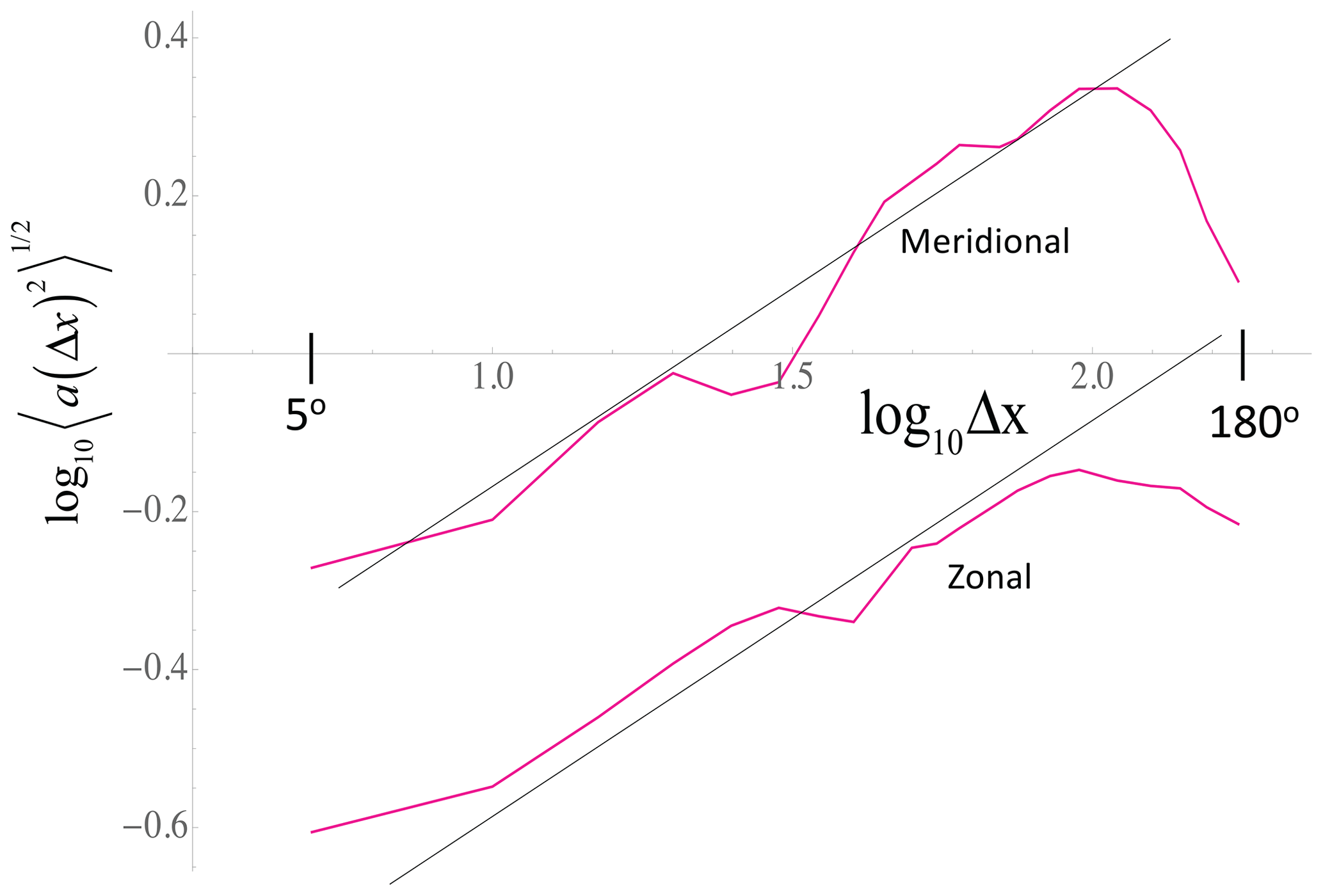
Figure A1 The rms fluctuations (at Δt= 1 month resolution) Δlog s_Δt(Δx) (zonal, bottom) and Δlog s_Δt(Δy) (meridional, top) from NCAR reanalyses. The vertical scale is dimensionless, and the horizontal scale is in log₁₀ (degrees) with the minimum (5^∘) and maximum (180^∘) indicated in large, bold font. The black lines are reference lines (not regressions) with slopes $H_x=H_y=$ 0.5.

Table A1 summarizes the dimensional and nondimensional parameter estimates; the final step is to estimate values of the gradient and Laplacian terms (Eq. A6). Since a – and hence log a – presents the amplitudes of temporal noises, these amplitudes vary stochastically from one spatial location to another. Due to the space–time scaling of the temperature anomalies (analyzed in Lovejoy and Schertzer, 2013), the statistics of the logarithms (Eq. A6) are expected to follow power laws up to large scales. To quantify this, I used NCEP reanalysis data at 2.5^∘ resolution from 1948 to the present. After removing the low-frequency anthropogenic trend, we estimated the rms temperature anomalies at each pixel, a(x). In Fig. A1, we then calculated spatial zonal and meridional fluctuations Δloga(Δx) and Δloga(Δy), and from these their root mean square (rms) values were calculated. From the figure, we see that to a good approximation,

$$\begin{array}{}\text{(A7)}& \begin{array}{rl}& \mathrm{\Delta }\log a\left(\mathrm{\Delta }x\right)\approx {\left({\displaystyle \frac{\mathrm{\Delta }x}{L_{\mathrm{EW}}}}\right)}^{H_x}\\ & \mathrm{\Delta }\log a\left(\mathrm{\Delta }y\right)={\left({\displaystyle \frac{\mathrm{\Delta }y}{L_{\mathrm{NS}}}}\right)}^{H_y}\\ & H_x\approx H_y\approx \mathrm{0.5};\\ & L_{\mathrm{NS}}\approx \mathrm{3}\times {\mathrm{10}}^{\mathrm{6}}\mathrm{m};L_{\mathrm{EW}}\approx \mathrm{1.5}\times {\mathrm{10}}^{\mathrm{7}}\mathrm{m};.\end{array}\end{array}$$

The fluctuations are Haar fluctuations, but because H_x≈H_y > 0, they are nearly equal to difference fluctuations (Lovejoy and Schertzer, 2012). We see that the zonal and meridional lines are roughly parallel, with a “trivial” horizontal anisotropy factor ≈ 5 (typical north–south fluctuations are 5 times larger than typical east–west ones). Although H= $\mathrm{1}/\mathrm{2}$ is the value corresponding to Brownian motion, the actual variability is highly intermittent (spiky), so unlike the temporal fluctuations, these spatial increments are far from Gaussian; it is not Brownian motion. Multifractal analysis indicates that the intermittency parameter (the codimension of the mean) C₁≈ 0.16, which is very high, reflecting the strong spatial fluctuations as we move from one climate zone to another (Lovejoy and Schertzer, 2013; Lovejoy, 2018; Lovejoy, 2019b).

Since the north–south gradients are much stronger than the east–west ones, it is sufficient to estimate the gradients and Laplacians by using only the y-direction fluctuations at scale Δy.

$$\begin{array}{}\text{(A8)}& {\displaystyle }{r}_{\mathrm{a},y}={\displaystyle \frac{V\mathit{\alpha }\mathrm{\Delta }t}{\mathrm{\Delta }y}}{\left({\displaystyle \frac{\mathrm{\Delta }y}{L_{\mathrm{NS}}}}\right)}^{H_y}\text{(A9)}& {\displaystyle }{r}_{d,y}={\displaystyle \frac{V\mathrm{\Delta }t}{\mathrm{\Delta }y}}\left({\displaystyle \frac{l_{\mathrm{h}}}{\mathrm{\Delta }y}}\right)\left[{\left({\displaystyle \frac{\mathrm{\Delta }y}{L_{\mathrm{NS}}}}\right)}^{\mathrm{2}{H}_y}+{\left({\displaystyle \frac{\mathrm{\Delta }y}{L_{\mathrm{NS}}}}\right)}^{H_y}\right]\end{array}$$

Since L_NS≈ 3× 10⁶ m over most of the range of Δy, $r_{d,y}\approx \frac{V\mathrm{\Delta }t}{\mathrm{\Delta }y}\left(\frac{l_{\mathrm{h}}}{\mathrm{\Delta }y}\right){\left(\frac{\mathrm{\Delta }y}{L_{\mathrm{NS}}}\right)}^{H_y}$, the ratio of advection to diffusion is $\frac{r_{\mathrm{c}}}{r_{\mathrm{d}}}\approx \left(\frac{\mathit{\alpha }\mathrm{\Delta }y}{l_{\mathrm{h}}}\right)$, so advection dominates diffusion for $\mathrm{\Delta }y>\frac{l_{\mathrm{h}}}{\mathit{\alpha }}$. Taking α≈ 1, it is dominant for $\mathrm{\Delta }y>\approx l_{\mathrm{h}}$.

Using l_h≈ 10⁴ m, L_NS≈ 3 × 10⁶ m, H_y= $\mathrm{1}/\mathrm{2}$, and V= 10⁻⁴ m/s, we find approximately critical length scales that yields unit ratios.

$$\begin{array}{}\text{(A10)}& \begin{array}{ll}\mathrm{\Delta }{y}_{\mathrm{c},\mathrm{a}}={\mathrm{10}}^{-\mathrm{14}}\mathrm{\Delta }{t}^{\mathrm{2}};& r_{\mathrm{a}}\left(\mathrm{\Delta }{y}_{\mathrm{c},\mathrm{a}}\right)=\mathrm{1}\\ \mathrm{\Delta }{y}_{\mathrm{c},\mathrm{d}}={\mathrm{10}}^{-\mathrm{2}}\mathrm{\Delta }{t}^{\mathrm{2}/\mathrm{3}};& r_{\mathrm{d}}\left(\mathrm{\Delta }{y}_{\mathrm{c},\mathrm{d}}\right)=\mathrm{1}\end{array}\end{array}$$

Δt is measured in seconds and Δy in meters. When the typical distances exceed these critical distances (i.e., when Δy > Δy_c), we have r < 1 so that the temporal derivative terms dominate over the horizontal transport. For Δt= 1 month, we have $\mathrm{\Delta }{y}_{\mathrm{c},\mathrm{a}}\approx$ 0.1 m and $\mathrm{\Delta }{y}_{\mathrm{c},\mathrm{d}}\approx$ 200 m, so unless the distances are very small, the temporal (storage) terms are indeed dominant. Even over much longer timescales, e.g., Δt≈ 30 years (10⁹ s), they dominate for distances greater than $\approx \mathrm{\Delta }{y}_{\mathrm{c},\mathrm{a}}\approx \mathrm{\Delta }{y}_{\mathrm{c},\mathrm{d}}$ ≈ 10 km.

Alternatively, we could estimate the timescales needed so that the critical transport scale is 1000 km. From the same equations, I obtain estimates of 300 years (advection) and 30 000 years (diffusion). Note, however, that in the Anthropocene, for periods Δt≈ > 10 years, the temporal fluctuations start to grow (i.e., the empirical relations in Eqs. A8 and A9 will break down); nevertheless, the above scaling relations for the internal variability may hold to much longer times (Lovejoy et al., 2013).

In summary, from Eq. (A10), I conclude that for the larger scales $\gg \approx$ 10 km, r≪ 1 and the HEBE may apply except for timescales ≫τ: the only explicit role of κ_h, κ_v, ρ, and c is to determine the limits of validity of the HEBE via l_h, α. When the HEBE is valid, only the relaxation time τ and the climate sensitivity s are relevant.

Appendix B: The HEBE cross-correlations

The temperature anomaly cross-correlation function (a matrix when the temperature is discretized on a grid) is commonly used in climate science, notably to determine empirical orthogonal functions (EOFs). These can be determined from the HEBE (or GHEBE if needed) once a forcing model is given. Let us first consider the climate sensitivities and relaxation times to be deterministic characterizations of the local properties at points x₁ and x₂. In this case, for the HEBE, any correlations between the temperature anomalies at those points will arise because of correlations in the forcing F(x,t). I now consider simple deterministic and stochastic forcings.

B1 (a) Deterministic forcing and temporal averaging

The simplest model is to take spatial correlations obtained by temporally averaging following a step function (Θ(t)) forcing at t= 0 but different at each position x:

$$\begin{array}{}\text{(B1)}& F(\mathit{x},t)=F_{\mathrm{0}}\left(\mathit{x}\right)\mathrm{\Theta }\left(t\right).\end{array}$$

The temporally averaged cross-correlation can be determined by

$$\begin{array}{}\text{(B2)}& \begin{array}{rl}& T({\mathit{x}}_{\mathrm{1}},t)T({\mathit{x}}_{\mathrm{2}},t)={\displaystyle \frac{s\left({\mathit{x}}_{\mathrm{1}}\right)F_{\mathrm{0}}\left({\mathit{x}}_{\mathrm{1}}\right)s\left({\mathit{x}}_{\mathrm{2}}\right)F_{\mathrm{0}}\left({\mathit{x}}_{\mathrm{2}}\right)}{\mathit{\tau }\left({\mathit{x}}_{\mathrm{1}}\right)\mathit{\tau }\left({\mathit{x}}_{\mathrm{2}}\right)}}\\ & \underset{\mathrm{0}}{\overset{t}{\int }}\underset{\mathrm{0}}{\overset{t}{\int }}{G}_{\mathit{\delta },\mathrm{1}/\mathrm{2}}\left({\displaystyle \frac{t-u_l}{\mathit{\tau }\left({\mathit{x}}_{\mathrm{1}}\right)}}\right)G_{\mathit{\delta },\mathrm{1}/\mathrm{2}}\left({\displaystyle \frac{t-u_{\mathrm{2}}}{\mathit{\tau }\left({\mathit{x}}_{\mathrm{2}}\right)}}\right)\mathrm{d}{u}_{\mathrm{1}}\mathrm{d}{u}_{\mathrm{2}}.\end{array}\end{array}$$

Recalling that the step response is the integral of $G_{\mathit{\delta },\mathrm{1}/\mathrm{2}}$ and since $G_{\mathrm{\Theta },\mathrm{1}/\mathrm{2}}\left(\mathrm{\infty }\right)=\mathrm{1}$, we have

$$\begin{array}{}\text{(B3)}& \underset{t_L\to \mathrm{\infty }}{lim}\left[{\displaystyle \frac{\mathrm{1}}{t_L}}\underset{\mathrm{0}}{\overset{t_L}{\int }}{G}_{\mathrm{\Theta },\mathrm{1}/\mathrm{2}}\left({\displaystyle \frac{t}{\mathit{\tau }\left({\mathit{x}}_{\mathrm{1}}\right)}}\right)G_{\mathrm{\Theta },\mathrm{1}/\mathrm{2}}\left({\displaystyle \frac{t}{\mathit{\tau }\left({\mathit{x}}_{\mathrm{2}}\right)}}\right)\mathrm{d}t\right]=\mathrm{1}.\end{array}$$

Hence,

$$\begin{array}{}\text{(B4)}& \stackrel{\mathrm{‾}}{T\left({\mathit{x}}_{\mathrm{1}},t\right)T\left({\mathit{x}}_{\mathrm{2}},t\right)}=s\left({\mathit{x}}_{\mathrm{1}}\right)F_{\mathrm{0}}\left({\mathit{x}}_{\mathrm{1}}\right)s\left({\mathit{x}}_{\mathrm{2}}\right)F_{\mathrm{0}}\left({\mathit{x}}_{\mathrm{2}}\right).\end{array}$$

B2 (b) Stochastic forcing

A convenient model of pure internal variability is to assume that the forcing is statistically stationary in time with the following forcing cross-correlations.

$$\begin{array}{}\text{(B5)}& R_F({\mathit{x}}_{\mathrm{1}},{\mathit{x}}_{\mathrm{2}},\mathrm{\Delta }t)=<F({\mathit{x}}_{\mathrm{1}},t)F({\mathit{x}}_{\mathrm{2}},t-\mathrm{\Delta }t)>\end{array}$$

The $<.>$ symbol indicates ensemble statistical averaging. The corresponding stationary temperature cross-correlation is

$$\begin{array}{}\text{(B6)}& R_T({\mathit{x}}_{\mathrm{1}},{\mathit{x}}_{\mathrm{2}},{\mathrm{\Delta }}_t)=<T({\mathit{x}}_{\mathrm{1}},t)T({\mathit{x}}_{\mathrm{2}},t-\mathit{\delta }t)>.\end{array}$$

Note the general symmetry property $R\left({\mathit{x}}_{\mathrm{1}},{\mathit{x}}_{\mathrm{2}},-\mathrm{\Delta }t\right)=R({\mathit{x}}_{\mathrm{2}},{\mathit{x}}_{\mathrm{1}},\mathrm{\Delta }t)$ so that we only need to determine R for Δt > 0. For statistically stationary forcing, $R_T({\mathit{x}}_{\mathrm{1}},{\mathit{x}}_{\mathrm{2}},\mathrm{\Delta }t)$ is the anomaly cross-correlation needed, for example, for constructing empirical orthogonal functions (EOFs).

The easiest way to relate R_F and R_T is via their spectra. Let us define the transform pairs as

$$\begin{array}{}\text{(B7)}& \widehat{T\left(\mathit{\omega }\right)}=\underset{-\mathrm{\infty }}{\overset{\mathrm{\infty }}{\int }}{e}^{-i\mathit{\omega }t}T\left(t\right)\mathrm{d}t;T\left(t\right)={\displaystyle \frac{\mathrm{1}}{\mathrm{2}\mathit{\pi }}}\underset{-\mathrm{\infty }}{\overset{\mathrm{\infty }}{\int }}{e}^{i\mathit{\omega }t}\widehat{T\left(\mathit{\omega }\right)}\mathrm{d}\mathit{\omega },\end{array}$$

similarly for the forcing F (the circumflex indicates Fourier transform). Then,

$$\begin{array}{}\text{(B8)}& \widehat{\left({\displaystyle \frac{d^{H}T}{\mathrm{d}{t}^H}}\right)}={\left(i\mathit{\omega }\right)}^H\widehat{T}.\end{array}$$

This is true for the Weyl fractional derivatives used here (Podlubny, 1999), so the impulse response is

$$\begin{array}{}\text{(B9)}& G_{\mathit{\delta },\mathrm{1}/\mathrm{2}}\left(t\right)={\displaystyle \frac{\mathrm{1}}{\mathrm{2}\mathit{\pi }}}\underset{-\mathrm{\infty }}{\overset{\mathrm{\infty }}{\int }}{\displaystyle \frac{e^{i\mathit{\omega }t}}{\mathrm{1}+{\left(i\mathit{\omega }\right)}^{\mathrm{1}/\mathrm{2}}}}\mathrm{d}\mathit{\omega }.\end{array}$$

The solution to the HEBE at two different points x₁ and x₂ is

$$\begin{array}{}\text{(B10)}& \begin{array}{rl}& \widehat{T}({\mathit{x}}_{\mathrm{1}},{\mathit{\omega }}_{\mathrm{1}})=s\left({\mathit{x}}_{\mathrm{1}}\right){\displaystyle \frac{\widehat{F}({\mathit{x}}_{\mathrm{1}},{\mathit{\omega }}_{\mathrm{1}})}{\mathrm{1}+\left(i{\mathit{\omega }}_{\mathrm{1}}\mathit{\tau }\right({\mathit{x}}_{\mathrm{1}}){)}^{\mathrm{1}/\mathrm{2}}}},\\ & {\widehat{T}}^{*}({\mathit{x}}_{\mathrm{2}},{\mathit{\omega }}_{\mathrm{2}})=s\left({\mathit{x}}_{\mathrm{2}}\right){\displaystyle \frac{\widehat{F^{*}}({\mathit{x}}_{\mathrm{2}},{\mathit{\omega }}_{\mathrm{2}})}{\mathrm{1}+(-i{\mathit{\omega }}_{\mathrm{2}}\mathit{\tau }({\mathit{x}}_{\mathrm{2}}){)}^{\mathrm{1}/\mathrm{2}}}},\end{array}\end{array}$$

where the asterisk indicates a complex conjugate. Multiplying, taking ensemble averages, and assuming that the forcing (and hence the response) is statistically stationary, we obtain

$$\begin{array}{}\text{(B11)}& \begin{array}{rl}\widehat{<T^{*}}({\mathit{x}}_{\mathrm{1}},\mathit{\omega })\widehat{T}({\mathit{x}}_{\mathrm{2}},{\mathit{\omega }}^{\prime })& >=\widehat{R_T}({\mathit{x}}_{\mathrm{1}},{\mathit{x}}_{\mathrm{2}},\mathit{\omega })\mathit{\delta }(\mathit{\omega }-{\mathit{\omega }}^{\prime });\\ & \widehat{R_T}({\mathit{x}}_{\mathrm{1}},{\mathit{x}}_{\mathrm{2}},\mathit{\omega })=\widehat{R_T^{*}}({\mathit{x}}_{\mathrm{2}},{\mathit{x}}_{\mathrm{1}},\mathit{\omega }),\end{array}\end{array}$$

where

$$\begin{array}{}\text{(B12)}& R_T({\mathit{x}}_{\mathrm{1}},{\mathit{x}}_{\mathrm{2}},\mathrm{\Delta }t)={\displaystyle \frac{\mathrm{1}}{\mathrm{2}\mathit{\pi }}}\underset{-\mathrm{\infty }}{\overset{\mathrm{\infty }}{\int }}{e}^{i\mathit{\omega }\mathrm{\Delta }t}{\widehat{R}}_T({\mathit{x}}_{\mathrm{1}},{\mathit{x}}_{\mathrm{2}},\mathit{\omega })\mathrm{d}\mathit{\omega }.\end{array}$$

Therefore,

$$\begin{array}{}\text{(B13)}& \begin{array}{rl}& R_T({\mathit{x}}_{\mathrm{1}},{\mathit{x}}_{\mathrm{2}},\mathit{\omega })=s\left({\mathit{x}}_{\mathrm{1}}\right)s\left({\mathit{x}}_{\mathrm{2}}\right){\widehat{G}}_T({\mathit{x}}_{\mathrm{1}},{\mathit{x}}_{\mathrm{2}},\mathit{\omega }){\widehat{R}}_F({\mathit{x}}_{\mathrm{1}},{\mathit{x}}_{\mathrm{2}},\mathit{\omega });\\ & {\widehat{G}}_T({\mathit{x}}_{\mathrm{1}},{\mathit{x}}_{\mathrm{2}},\mathit{\omega })={\displaystyle \frac{\mathrm{1}}{(\mathrm{1}+(-i\mathit{\omega }\mathit{\tau }\left({\mathit{x}}_{\mathrm{1}}\right){)}^{\mathrm{1}/\mathrm{2}}\left)\right(\mathrm{1}+\left(i\mathit{\omega }\mathit{\tau }\right({\mathit{x}}_{\mathrm{2}}\left){)}^{\mathrm{1}/\mathrm{2}}\right)}}.\end{array}\end{array}$$

A special case that is useful later is when ${\mathit{x}}_{\mathrm{1}}={\mathit{x}}_{\mathrm{2}}=\mathit{x}$, which yields the spectrum E_T at the point x:

$$\begin{array}{}\text{(B14)}& \begin{array}{rl}& E_T(\mathit{x},\mathit{\omega })\mathit{\delta }(\mathit{\omega }-{\mathit{\omega }}^{\prime })=\langle \widehat{T}(\mathit{x},\mathit{\omega })\widehat{T^{*}}(\mathit{x},{\mathit{\omega }}^{\prime })\rangle ;\\ & E_T(\mathit{x},\mathit{\omega })={\widehat{R}}_T(\mathit{x},\mathit{x},\mathit{\omega }).\end{array}\end{array}$$

Using a partial fraction expansion of Eq. (B13), we obtain

$$\begin{array}{}\text{(B15)}& \begin{array}{rl}{\widehat{G}}_T& ({\mathit{x}}_{\mathrm{1}},{\mathit{x}}_{\mathrm{2}},\mathrm{\Delta }t)\\ & ={\displaystyle \frac{\mathrm{1}}{{\mathit{\tau }}_{\mathrm{1}}+{\mathit{\tau }}_{\mathrm{2}}}}\left[{\displaystyle \frac{{\mathit{\tau }}_{\mathrm{1}}+i{\mathit{\tau }}_g}{(\mathrm{1}+(-i\mathit{\omega }{\mathit{\tau }}_{\mathrm{1}}{)}^{\mathrm{1}/\mathrm{2}})}}+{\displaystyle \frac{{\mathit{\tau }}_{\mathrm{2}}-i{\mathit{\tau }}_g}{(\mathrm{1}+(i\mathit{\omega }{\mathit{\tau }}_{\mathrm{2}}{)}^{\mathrm{1}/\mathrm{2}})}}\right];\\ & {\mathit{\tau }}_g=\mathrm{sign}\left(\mathit{\omega }\right)({\mathit{\tau }}_{\mathrm{1}}{\mathit{\tau }}_{\mathrm{2}}{)}^{\mathrm{1}/\mathrm{2}}.\end{array}\end{array}$$

By inverting the Fourier transform, this can be used to determine the real space transfer function $G_T({\mathit{x}}_{\mathrm{1}},{\mathit{x}}_{\mathrm{2}},\mathrm{\Delta }t)$. Using contour integration, it is convenient to convert the inverse Fourier transforms into Laplace transforms for Δt > 0.

$$\begin{array}{}\text{(B16)}& \begin{array}{rl}{G}_T({\mathit{x}}_{\mathrm{1}},{\mathit{x}}_{\mathrm{2}},\mathrm{\Delta }t)=& {\displaystyle \frac{\mathrm{1}}{\mathit{\pi }({\mathit{\tau }}_{\mathrm{1}}+{\mathit{\tau }}_{\mathrm{2}})}}\\ & \left[\underset{\mathrm{0}}{\overset{\mathrm{\infty }}{\int }}{e}^{-x(\mathrm{\Delta }t/{\mathit{\tau }}_{\mathrm{2}})}{\displaystyle \frac{x^{\mathrm{1}/\mathrm{2}}}{\mathrm{1}+x}}\mathrm{d}x+{\left({\displaystyle \frac{{\mathit{\tau }}_{\mathrm{2}}}{{\mathit{\tau }}_{\mathrm{1}}}}\right)}^{\mathrm{1}/\mathrm{2}}\right.\\ & \underset{\mathrm{0}}{\overset{\mathrm{\infty }}{\int }}{e}^{-x(\mathrm{\Delta }t/{\mathit{\tau }}_{\mathrm{2}})}{\displaystyle \frac{\mathrm{1}}{\mathrm{1}+x}}\mathrm{d}x{\left({\displaystyle \frac{{\mathit{\tau }}_{\mathrm{1}}}{{\mathit{\tau }}_{\mathrm{2}}}}\right)}^{\mathrm{1}/\mathrm{2}}\\ & \left.\underset{\mathrm{0}}{\overset{\mathrm{\infty }}{\int }}{e}^{-\mathrm{1}x(\mathrm{\Delta }t/{\mathit{\tau }}_{\mathrm{1}})}{\displaystyle \frac{\mathrm{1}}{\mathrm{1}+x^{\mathrm{1}/\mathrm{2}}}}\mathrm{d}x\right]\end{array}\end{array}$$

For Δt < 0, use $G_T({\mathit{x}}_{\mathrm{1}},{\mathit{x}}_{\mathrm{2}},-\mathrm{\Delta }t)=G_T({\mathit{x}}_{\mathrm{2}},{\mathit{x}}_{\mathrm{1}},\mathrm{\Delta }t))$. The spatial cross-correlation, or the temporal autocorrelation function of the temperature, is therefore

$$\begin{array}{}\text{(B17)}& \begin{array}{rl}{R}_T& ({\mathit{x}}_{\mathrm{1}},{\mathit{x}}_{\mathrm{2}},\mathrm{\Delta }t)=s\left({\mathit{x}}_{\mathrm{1}}\right)s\left({\mathit{x}}_{\mathrm{2}}\right)G_T({\mathit{x}}_{\mathrm{1}},{\mathit{x}}_{\mathrm{2}},\mathrm{\Delta }t)\\ & *R_F({\mathit{x}}_{\mathrm{1}},{\mathit{x}}_{\mathrm{2}},\mathrm{\Delta }t),\end{array}\end{array}$$

where the * symbol indicates convolution.

The basic Laplace transforms in Eq. (B16) can be expressed in terms of higher mathematical functions as follows (all for t > 0).

$$\begin{array}{}\text{(B18)}& G_{\mathit{\delta },\mathrm{1}/\mathrm{2}}\left(t\right)={\displaystyle \frac{\mathrm{1}}{\mathit{\pi }}}\underset{\mathrm{0}}{\overset{\mathrm{\infty }}{\int }}{\displaystyle \frac{x^{\mathrm{1}/\mathrm{2}}}{\mathrm{1}+x}}{e}^{-xt}\mathrm{d}x={\displaystyle \frac{\mathrm{1}}{\sqrt{\mathit{\pi }t}}}-e^t\mathrm{erfc}\left(\sqrt{t}\right)\end{array}$$

$$\begin{array}{ll}{\displaystyle }& {\displaystyle }\begin{array}{l}\frac{\mathrm{1}}{\mathit{\pi }}\underset{-}{\overset{\mathrm{\infty }}{\int }}\frac{e^{-xt}}{\mathrm{1}+x}\mathrm{d}x=\frac{\mathrm{1}}{\mathit{\pi }}{e}^t\mathrm{\Gamma }(\mathrm{0},t);\mathrm{\Gamma }(\mathrm{0},t)=\underset{t}{\overset{\mathrm{\infty }}{\int }}\frac{e^{-t}}{t}\mathrm{d}t\\ {\displaystyle \frac{\mathrm{1}}{\mathit{\pi }}}\underset{\mathrm{0}}{\overset{\mathrm{\infty }}{\int }}{\displaystyle \frac{\mathrm{1}}{\mathrm{1}+x^{\mathrm{1}/\mathrm{2}}}}{e}^{-xt}\mathrm{d}x={\displaystyle \frac{\mathrm{1}}{\sqrt{\mathit{\pi }t}}}-e^{-t}\mathrm{erfi}\left(\sqrt{t}\right)+{\displaystyle \frac{e^{-t}}{\mathit{\pi }}}{E}_I\left(t\right);\end{array}\\ {\displaystyle }& {\displaystyle }\begin{array}{l}\mathrm{erfi}\left(x\right)=\mathrm{erf}\left(iz\right)/i=\mathrm{Im}\left(\mathrm{erfc}\right(-iz\left)\right);\\ E_I=\underset{-t}{\overset{\mathrm{\infty }}{\int }}{\displaystyle \frac{e^{-t}}{t}}\mathrm{d}t=-\mathrm{\Gamma }(\mathrm{0},t)+i\mathit{\pi }\end{array}\end{array}$$

The iπ comes from integrating halfway around the pole at the origin. Note that both the exponential integral (E_I) and the incomplete Gamma functions have log divergences at the origin. If needed, these formulae can be combined to obtain a complete analytic expression for $G_T\left({\mathit{x}}_{\mathrm{1}},{\mathit{x}}_{\mathrm{2}},\mathrm{\Delta }t\right)$, which can then be used to determine the temperature correlations if the forcing correlations are known: $R_T({\mathit{x}}_{\mathrm{1}},{\mathit{x}}_{\mathrm{2}},\mathrm{\Delta }t)=s\left({\mathit{x}}_{\mathrm{1}}\right)s\left({\mathit{x}}_{\mathrm{2}}\right)G_T({\mathit{x}}_{\mathrm{1}},{\mathit{x}}_{\mathrm{2}},\mathrm{\Delta }t)*R_F({\mathit{x}}_{\mathrm{1}},{\mathit{x}}_{\mathrm{2}},\mathrm{\Delta }t)$, where the asterisk is the temporal convolution.

The special case x₁=x₂, i.e., with ${\mathit{\tau }}_{\mathrm{1}}={\mathit{\tau }}_{\mathrm{2}}=\mathit{\tau }$, is a little simpler:

$$\begin{array}{}\text{(B19)}& \begin{array}{rl}{G}_T& \left(\mathrm{\Delta }t\right)={\displaystyle \frac{\mathrm{1}}{\mathit{\tau }}}g\left({\displaystyle \frac{\left|\mathrm{\Delta }t\right|}{\mathit{\tau }}}\right);\\ & g\left(\mathrm{\Delta }t\right)={\displaystyle \frac{\mathrm{1}}{\mathrm{2}\mathit{\pi }}}\underset{\mathrm{0}}{\overset{\mathrm{\infty }}{\int }}{e}^{-x\mathrm{\Delta }t}\left({\displaystyle \frac{x^{\mathrm{1}/\mathrm{2}}}{\mathrm{1}+x}}+{\displaystyle \frac{\mathrm{1}}{\mathrm{1}+x}}-{\displaystyle \frac{\mathrm{1}}{\mathrm{1}+x^{\mathrm{1}/\mathrm{2}}}}\right)\mathrm{d}x;\\ & \mathrm{\Delta }t>\mathrm{0},\end{array}\end{array}$$

whose Fourier transform is

$$\begin{array}{}\text{(B20)}& {\widehat{G}}_T(\mathit{x},\mathit{x},\mathit{\omega })={\displaystyle \frac{\mathrm{1}}{\mathrm{1}+\mathrm{2}\mathit{Re}\left[\right(-i\mathit{\omega }\mathit{\tau }{)}^{\mathrm{1}/\mathrm{2}}]+\mathit{\omega }\mathit{\tau }}}.\end{array}$$

Evaluating the integral for g(Δt) using the Laplace transform formulae (Eq. B18), we have the following.

$$\begin{array}{}\text{(B21)}& \begin{array}{rl}g\left(\mathrm{\Delta }t\right)& ={\displaystyle \frac{\mathrm{1}}{\mathit{\pi }}}\left(e^{\mathrm{\Delta }t}\mathrm{\Gamma }\left(\mathrm{0},\mathrm{\Delta }t\right)+e^{-\mathrm{\Delta }t}\mathit{Re}\left(\mathrm{\Gamma }\left(\mathrm{0},-\mathrm{\Delta }t\right)\right)\right)\\ & -\left(e^{\mathrm{\Delta }t}\mathrm{erfc}\sqrt{\mathrm{\Delta }t}+e^{-\mathrm{\Delta }t}\mathrm{Im}\left(\mathrm{erfc}\left(-i\sqrt{\mathrm{\Delta }t}\right)\right)\right)\end{array}\end{array}$$

Here, Δt > 0. The small-scale and asymptotic limits are thus as follows.

$$\begin{array}{}\text{(B22)}& \begin{array}{rl}g\left(\mathrm{\Delta }t\right)& =-{\displaystyle \frac{\log \mathrm{\Delta }t}{\mathit{\pi }}}-{\displaystyle \frac{\mathrm{1}}{\mathrm{2}}}-{\displaystyle \frac{{\mathit{\gamma }}_E}{\mathit{\pi }}}+\mathrm{2}\sqrt{{\displaystyle \frac{\mathrm{\Delta }t}{\mathit{\pi }}}}-{\displaystyle \frac{t}{\mathrm{2}}}\\ & -\left({\displaystyle \frac{t^{\mathrm{2}}\log \mathrm{\Delta }t}{\mathrm{2}\mathit{\pi }}}\right)+\mathrm{\dots }\mathrm{\Delta }t\ll \mathrm{1}\\ g\left(\mathrm{\Delta }t\right)& \approx {\displaystyle \frac{\mathrm{1}}{\mathrm{\Delta }t\sqrt{\mathit{\pi }\mathrm{\Delta }t}}}-{\displaystyle \frac{\mathrm{2}}{\mathit{\pi }\mathrm{\Delta }{t}^{\mathrm{2}}}}+{\displaystyle \frac{\mathrm{15}}{\mathrm{8}\mathrm{\Delta }{t}^{\mathrm{3}}\sqrt{\mathit{\pi }\mathrm{\Delta }t}}}-\mathrm{\dots }\mathrm{\Delta }t\mathit{>>}\mathrm{1}\end{array}\end{array}$$

Note the small-scale log divergence because this is important when the forcing is white noise; see Lovejoy (2019a). The temporal autocorrelation at the point x is thus

$$\begin{array}{}\text{(B23)}& \begin{array}{rl}{R}_T(\mathit{x},\mathrm{\Delta }t)=& {\displaystyle \frac{s(\mathit{x}{)}^{\mathrm{2}}}{\mathit{\tau }\left(\mathit{x}\right)}}g(\mathrm{\Delta }t/\mathit{\tau }(\mathit{x}\left)\right)*R_F(\mathit{x},\mathrm{\Delta },t);\\ & R(x,\mathrm{\Delta }t)=R(\mathit{x},\mathit{x},\mathrm{\Delta }t).\end{array}\end{array}$$

However, in general, the Fourier relations are easier to deal with.

Appendix C: Fractional integration on the sphere

At long enough timescales, the spatial transport of heat is important and the spherical geometry of the Earth must be taken into account. The standard way (see Sect. 2.3 and the reviews in North et al., 1981; North and Kim, 2017) is to use spherical harmonics. In Appendix 5D of Lovejoy and Schertzer (2013) these were used to define fractional integrals on the sphere, which is necessary in order to produce the corresponding multifractal cloud and topography models (see also Landais et al., 2019). Spherical harmonics are particularly convenient when the heat transport is diffusive, involving fractional Laplacians. In Sect. 3.5.2, these were defined in real space by taking the domain of integration to be a sphere. In this Appendix I discuss an alternative method of spherical fractional integration that may have theoretical and practical advantages.

The Laplacian on a sphere (${\mathrm{\nabla }}_{\mathrm{\Omega }}^{\mathrm{2}}$) is the angular part of the Laplacian in spherical coordinates; it is obtained by expressing the Laplacian in spherical coordinates and setting the radial derivatives to zero:

$$\begin{array}{}\text{(C1)}& {\mathrm{\nabla }}_{\mathrm{\Omega }}^{\mathrm{2}}=\left[{\displaystyle \frac{\partial }{\partial \mathit{\mu }}}\left(\mathrm{1}-{\mathit{\mu }}^{\mathrm{2}}\right){\displaystyle \frac{\partial }{\partial \mathit{\mu }}}+{\displaystyle \frac{\mathrm{1}}{\left(\mathrm{1}-{\mathit{\mu }}^{\mathrm{2}}\right)}}{\displaystyle \frac{{\partial }^{\mathrm{2}}}{\partial {\mathit{\varphi }}^{\mathrm{2}}}}\right];\mathit{\mu }=\cos \mathit{\theta },\end{array}$$

where θ is the colatitude and φ is the longitude. The normalized eigenfunctions of ${\mathrm{\nabla }}_{\mathrm{\Omega }}^{\mathrm{2}}$ are the spherical harmonics Y_n,m:

$$\begin{array}{}\text{(C2)}& \begin{array}{rl}{Y}_{n,m}\left(\mathit{\mu },\mathit{\varphi }\right)=& {\left[{\displaystyle \frac{\mathrm{2}n+\mathrm{1}}{\mathrm{4}\mathit{\pi }}}{\displaystyle \frac{\left(n-\left|m\right|\right)\mathrm{!}}{\left(n+\left|m\right|\right)\mathrm{!}}}\right]}^{\mathrm{1}/\mathrm{2}}{P}_{n,\left|m\right|}\left(\mathit{\mu }\right)e^{im\mathit{\varphi }}\\ & \left(\begin{array}{ll}{\left(-\mathrm{1}\right)}^m;& m\ge \mathrm{0}\\ \mathrm{1};& m<\mathrm{0}\end{array}\right);\mathit{\mu }=\cos \mathit{\theta };\\ & -n\le m\le n,\end{array}\end{array}$$

with m and n as integers; n≥ 0, and P_n,m represents the associated Legendre polynomials. Y_n,m satisfies

$$\begin{array}{}\text{(C3)}& -{\mathrm{\nabla }}_{\mathrm{\Omega }}^{\mathrm{2}}{Y}_{n,m}\left(\mathit{\mu },\mathit{\varphi }\right)=n\left(n+\mathrm{1}\right)Y_{n,m}\left(\mathit{\mu },\mathit{\varphi }\right)\end{array}$$

so that n(n+1) represents the eigenvalues. Since |m|≤n there are 2n+1 degenerate eigenvalues and functions for each n.

The spherical harmonics form a complete orthogonal basis so that any function f(μ,ϕ) on the sphere can be uniquely expressed in terms of a spherical harmonic expansion:

$$\begin{array}{}\text{(C4)}& \begin{array}{rl}& f\left(\mathit{\mu },\mathit{\varphi }\right)=\sum _{n=\mathrm{0}}^{\mathrm{\infty }}\sum _{m=-n}^n{F}_{n,m}^{\left(\mathrm{0}\right)}{Y}_{n,m}\left(\mathit{\mu },\mathit{\varphi }\right);\\ & F_{n,m}^{\left(\mathrm{0}\right)}=\underset{\mathrm{0}}{\overset{\mathrm{2}\mathit{\pi }}{\int }}\underset{-\mathrm{1}}{\overset{\mathrm{1}}{\int }}{Y}_{n,m}^{*}\left(\mathit{\mu },\mathit{\varphi }\right)f\left(\mathit{\mu },\mathit{\varphi }\right)\mathrm{d}\mathit{\mu }\mathrm{d}\mathit{\varphi },\end{array}\end{array}$$

where $F_{n,m}^{\left(\mathrm{0}\right)}$ represents the coefficients of the expansion without fractional integration (i.e., of order 0, indicated in the superscript). This suggests the following definition for a fractional spherical integration order h of a spherical harmonic:

$$\begin{array}{}\text{(C5)}& {\left(-{\mathrm{\nabla }}_{\mathrm{\Omega }}^{\mathrm{2}}\right)}^{-h/\mathrm{2}}{Y}_{n,m}\left(\mathit{\mu }\right)={\left[n\left(n+\mathrm{1}\right)\right]}^{-h/\mathrm{2}}{Y}_{n,m}\left(\mathit{\mu }\right);n\ge \mathrm{1}.\end{array}$$

For the HEBE, take h= 1, which corresponds to the $\mathrm{1}/\mathrm{2}$ power of the inverse Laplacian (see Sect. 2.3 for the zonally averaged case that depends only on n). I have excluded the value n= 0 since when h > 0, the filter ${\left[n\left(n+\mathrm{1}\right)\right]}^{-h/\mathrm{2}}$ diverges; since $Y_{\mathrm{0},\mathrm{0}}\left(\mathit{\mu },\mathit{\varphi }\right)=\frac{\mathrm{1}}{\sqrt{\mathrm{4}\mathit{\pi }}}$, this component corresponds to the mean. Therefore, the above definition is only adequate for mean zero anomalies. Alternatively, the mean can be removed and taken care of separately; see below. With this definition, the fractional integral of the zero mean function f is

$$\begin{array}{}\text{(C6)}& \begin{array}{rl}& {\left(-{\mathrm{\nabla }}_{\mathrm{\Omega }}^{\mathrm{2}}\right)}^{-h/\mathrm{2}}f\left(\mathit{\mu },\mathit{\varphi }\right)=\sum _{n=\mathrm{1}}^{\mathrm{\infty }}\sum _{m=-n}^n{F}_{n,m}^{\left(h\right)}{Y}_{n,m}\left(\mathit{\mu },\mathit{\varphi }\right);\\ & F_{n,m}^{\left(h\right)}={\left[n\left(n+\mathrm{1}\right)\right]}^{-h/\mathrm{2}}{F}_{n,m}^{\left(\mathrm{0}\right)},\end{array}\end{array}$$

i.e., a filter in spherical harmonic space, analogous to the Fourier filter |k|^−h for an isotropic fractional integration in Cartesian coordinates.

The definition of the fractional Laplacian (Eqs. C5, C6) is adequate when the horizontal transport coefficients are constant, but in Sect. 3.5 we saw that, more generally, the half-order divergence operator was written as $l{\left(\mathit{\mu },\mathit{\varphi }\right)}^{-\mathrm{1}}{\left(-{\mathrm{\nabla }}_{\mathrm{\Omega }}^{\mathrm{2}}\right)}^{-\mathrm{1}/\mathrm{2}}$; i.e., there was an extra multiplication by the spatially varying diffusion length l(μ,ϕ). In flat (Cartesian) coordinates, such real space multiplications correspond to Fourier space convolutions so that this operator can also be conveniently expressed in Fourier space. However, with spherical harmonics, this simplicity is lost: although isotropic real space convolutions can still be performed by filtering the harmonics, real space multiplications no longer correspond to convolutions of harmonic coefficients, and the closest spherical harmonic equivalent is much more complicated; it involves Clebsch–Gordan coefficients.

A method of fractionally integrating the mean (n= 0) component was developed for the purpose of multifractal modeling in Appendix 5D of Lovejoy and Schertzer (2013). There, a different definition of fractional integrals on the sphere was proposed: a convolution with the function ${\mathrm{\Theta }}^{-(\mathrm{2}-h)}$, where Θ is the angle between two points subtended at the center of the sphere. The function ${\mathrm{\Theta }}^{-(\mathrm{2}-h)}/\mathrm{\Gamma }(h/\mathrm{2})$ was numerically expanded in spherical harmonics and the convolution was again performed by filtering the coefficients (the constant $\mathrm{\Gamma }(h/\mathrm{2}$) is needed so that the normalization is the same as for the definition in Eq. C4). The main difference between the two definitions is that the latter can be directly applied to fields with nonzero means. With this definition, the h-order fractional integral of a constant function on the sphere (representing the nonzero mean) is simply the value multiplied by ${\mathrm{2}}^{-h/\mathrm{2}}\sqrt{\mathit{\pi }}/\mathrm{\Gamma }\left(h/\mathrm{2}\right)\underset{\mathrm{0}}{\overset{\mathrm{2}\mathit{\pi }}{\int }}{s}^{-\left(\mathrm{2}-h\right)}\sin s\mathrm{d}s$, which for the HEBE h= 1 case reduces to (1/2)${}^{\mathrm{1}/\mathrm{2}}$ Si(2π), where Si is the standard sine integral function. However, for the coefficients n≥1, numerical tests show that the two definitions are almost exactly the same; for example, with h= 1, the spherical harmonic coefficients of ${\mathrm{\Theta }}^{-(\mathrm{2}-h)}$ are within 3 % for all n≥ 1 and the ratio converges rapidly to 1 for large n. The conclusion is that filtering the anomaly by ${\left[n\left(n+\mathrm{1}\right)\right]}^{-h/\mathrm{2}}$ and then multiplying the mean by the above factor is a practical method of fractionally integrating a function on the sphere.