Spatiotemporal patterns of synchronous heavy rainfall events in East Asia during the Baiu season

Investigating the synchrony and interdependency of heavy rainfall occurrences is crucial to understand the underlying physical mechanisms and reduce physical and economic damages by improved forecasting strategies. In this context, studies utilizing functional network representations have recently contributed to significant advances in the understanding and prediction of extreme weather events. To thoroughly expand on previous works employing the latter framework to the East Asian summer monsoon (EASM) system, we focus here on changes in the spatial organization of synchronous heavy precipitation events across the monsoon season (April to August) by studying the temporal evolution of corresponding network characteristics in terms of a sliding window approach. Specifically, we utilize functional climate networks together with event coincidence analysis for identifying and characterizing synchronous activity from daily rainfall estimates between 1998 and 2018. Our results demonstrate that the formation of the Baiu front as a main feature of the EASM is reflected by a double-band structure of synchronous heavy rainfall with two centers north and south of the front. Although the two separated bands are strongly related to either low- or high-level winds, which are commonly assumed to be independent, we provide evidence that it is rather their mutual interconnectivity that changes during the different phases of the EASM season in a characteristic way. Our findings shed some new light on the interplay between tropical and extratropical factors controlling the EASM intraseasonal evolution, which could potentially help to improve future forecasts of the Baiu onset in different regions of East Asia.

1 Introduction

The Asian summer monsoon dominates the rainfall pattern over South and East Asia, thereby impacting nearly a third of the world's population. Disregarding the western (Arabian Sea) branch of the Indian summer monsoon (ISM), this major weather system is mainly initiated over Southeast Asia and the maritime continent, from which one branch expands westward to the Bay of Bengal and eastern Indian Ocean, forming the eastern branch of the ISM (Yihui and Chan, 2005). A second branch, the East Asian summer monsoon (EASM), progressively moves northward along the western edge of the Northwest Pacific Subtropical High (NPSH) following the gradual northward migration of the upper-level jet (Suda and Asakura, 1955; Okada and Yamazaki, 2012). The main EASM-related frontal pattern largely contributes to the annual rainfall over the Philippines and China (as Meiyu), Korean peninsula (as Changma), and Japan (as Baiu) during May, June, and July (Fukui, 1970; Preethi et al., 2017; Li et al., 2018) and will be simply referred to as the Baiu season in the rest of this work. A physical map of the region affected by the Baiu front, which corresponds to the study region of the analysis to be presented in this paper, can be found in Fig. 1.

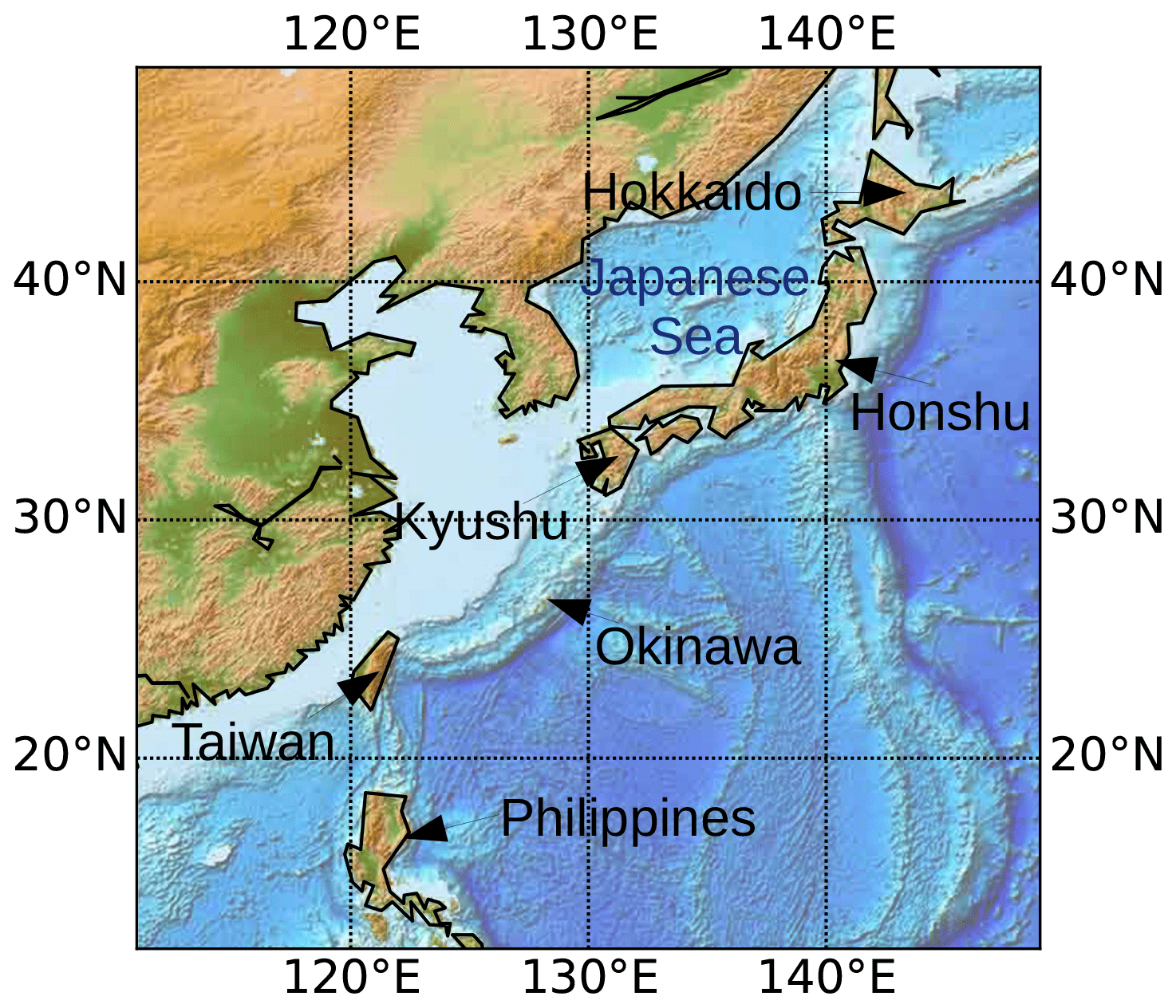
Figure 1 Physical map of the study region, including references to the most relevant geographical aspects mentioned in the text.

The Baiu front extends east-to-northeastward from the Tibetan Plateau towards the western Pacific Ocean over southern Japan, linking Arctic and tropical circulation patterns, where cool polar maritime air masses intersect with warm maritime tropical air (Sampe and Xie, 2010). The resulting quasi-stationary subtropical frontal zone gradually expands and progressively shifts northward from Taiwan (25^∘ N) up to western Japan (40^∘ N) in about 40 d. The tropical western Pacific, the South China Sea, and the Bay of Bengal supply the moisture that propagates eastward along the front with the middle and upper tropospheric circulations (Ninomiya and Muraki, 1986; Krishnan and Sugi, 2001). The front retreats are associated with the convective activity over the northwestern Pacific and the northward shift of the NPSH from late July onward (Ninomiya and Muraki, 1986; Ueda and Yasunari, 1995; Okada and Yamazaki, 2012). The onset and strength of Baiu vary on an interannual basis (Zhu et al., 2013), which reduces its predictability via repetitive atmospheric circulation systems associated with large-scale teleconnection patterns like the Antarctic Oscillation, South Asian Anticyclone (SAA), and El Niño–Southern Oscillation (Zhu et al., 2008; Choi et al., 2012; Li et al., 2018).

The dynamical organization of particularly heavy rainfall events across the EASM domain is relevant in the context of anticipating and mitigating corresponding natural disasters like flash floods or landslides. In a related context, Wang et al. (2019) have recently pointed to a considerable likelihood of consecutive extreme flood and heat wave events in Japan (like those observed in July 2018), which further emphasizes the need to better understand the emergence of such situations. Moreover, being able to accurately predict the onset of the Baiu frontal system could heavily impact the agricultural activities in the affected regions that ultimately depend on water supply by the associated heavy (yet not necessarily the most severe) downpours but requires further improvement of our understanding of EASM in terms of both its external controls and internal dynamics.

Addressing the aforementioned problems is complicated by the fact that the spatiotemporal organization of heavy rainfall in monsoon-dominated regions is very complex. Therefore, disentangling the governing processes across time and space requires specific statistical and dynamical approaches that are not part of the classical toolbox of statistical climatology. For the specific situation in East Asia, it has to be noted that in addition to monsoon-related heavy rainfall resulting from the internal Baiu dynamics, typhoons constitute another type of phenomena that are often associated with such events. The spatiotemporal dynamics of heavy rainfall associated with typhoons has been recently studied by Ozturk et al. (2018, 2019) with methods originating from the field of complex networks. Similar functional network representations of climate variability (Tsonis and Roebber, 2004; Donges et al., 2009; Donner et al., 2017; Dijkstra et al., 2019) have already been successfully used in past works to identify regions where heavy rainfall coherently occurs over considerably large spatial regions, e.g., in the context of the ISM (Malik et al., 2010, 2012; Stolbova et al., 2014), the South American Monsoon System (SAMS) (Boers et al., 2013, 2014b; Gelbrecht et al., 2018), or the Australian summer monsoon (Cheung and Ozturk, 2020). For the EASM, an initial study employing a network-based analysis (He et al., 2014) has only recently been complemented by further research, revealing a distinct precipitation pattern for the Baiu and typhoon seasons over Japan (Ozturk et al., 2019). This growing body of literature, together with a vast amount of additional climate-network-based studies not focusing explicitly on extreme events (see, e.g., Donner et al., 2017; Dijkstra et al., 2019, for some recent overviews), indicates that this approach has great potential for contributing to a better understanding of the spatiotemporal organization of climate variability in general and heavy precipitation events in particular.

In this work, we focus on the Baiu-related heavy rainfall events and do not explicitly consider the effect of tropical cyclones. Moreover, we expand the study area of Ozturk et al. (2019) beyond the core Baiu frontal region to better characterize large-scale synchronous occurrences of heavy rainfall events along with the progress of the Baiu season. Specifically, we explore the temporal evolution of Baiu-associated coherent heavy rainfall events over an extended spatial region covering vast parts of East Asia and the adjacent western Pacific Ocean (10–50^∘ N, 110–150^∘ E) and an enlarged time period between April and August also including the initiation and withdrawal phases of the Baiu front. We employ event coincidence analysis (ECA) (Donges et al., 2016) to measure the synchrony of heavy rainfall events at different sites and use the associated similarity measure to construct functional climate networks (Odenweller and Donner, 2020; Wolf et al., 2020), two key topological properties of which are then thoroughly studied. Our corresponding analysis identifies two particular regions of synchronously occurring heavy rainfall events north and south of the Baiu front, the evolving mutual connectivity of which across the Baiu season is further studied by utilizing a sliding window approach. Finally, we discuss our complex network-based findings in the context of various meteorological variables characterizing different aspects of the atmospheric circulation in the study region.

2 Data and methods

2.1 Data

For studying the spatio-temporal patterns of heavy rainfall events over East Asia, we employ daily rainfall estimates from the Tropical Rainfall Measurement Mission (TRMM, version 3B42 V7) (TRMM, 2011), which are available on a $\mathrm{0.25}{}^{\circ }\times \mathrm{0.25}{}^{\circ }$ spatial grid between 1998 and 2018. This data set has been chosen here due to its high spatial and temporal resolution, but exhibits the disadvantage of potential biases in comparison with other gauged precipitation products. However, for the purpose of the present study, we are not interested in the exact rainfall sums, but exclusively in the timing of the strongest rainfall days for each grid point individually (see below) – a type of information that would not be affected by the aforementioned biases as long as the latter depend at most on precipitation magnitude and geographical location but do not change with time.

In the following, we consider rainfall to be heavy if a corresponding daily value exceeds the 90th percentile of all daily values for a given grid point. This percentile provides a typical value used in previous studies on similar topics, which guarantees a sufficient number of events for proper statistical analysis while still focusing on a minority of days with extraordinary strong rainfall. By proceeding as described we obtain the same number of heavy precipitation events in almost all grid point time series and only ignore dry spots, where an insufficiently low number of rainy days has been observed during the respective study period.

Instead of taking precipitation values for the entire year, for our analysis we only consider rainfall during a certain period, which we specify in the respective parts of Sect. 3. In each case, we select a proper time window and take the respective days of this window in every year into account. Thus, we stack all time series segments containing precipitation values of, e.g., all days in April at each individual data point, while taking into account in our analysis (see below) that events from late April in a single year cannot be dynamically related with events in early April of the following year.

In order to better understand the climatological background of the obtained precipitation pattern, we perform a complementary synoptic analysis based on data from the US National Center for Environmental Prediction/National Center for Atmospheric Research (NCEP/NCAR) Reanalysis version 1 and the National Center for Environmental Prediction–Department of Energy (NCEP-DOE) Reanalysis version 2 (Kalnay et al., 1996; Kanamitsu et al., 2002), referred to as R1 and R2 in the following, respectively. R1 and R2 are global reanalysis data sets with a 2.5^∘ latitude–longitude resolution. To match with the analysis of heavy rainfall from TRMM, we employ the geopotential height, specific humidity, and horizontal and vertical wind fields (and the derived relative vorticity) from R1 (daily data, used for producing Figs. 8–10) and R2 (monthly data, used for producing Fig. 7) for the period 1998–2018. In addition, outgoing longwave radiation (OLR) from the US National Oceanic and Atmospheric Administration (NOAA) is examined as a proxy for convection.

2.2 Event coincidence analysis (ECA)

ECA (Donges et al., 2011, 2016) is a statistical method for investigating synchrony of events in pairs of time series, which has recently been applied for studying spatiotemporal climate variability patterns by means of a functional network approach as described below (Odenweller and Donner, 2020; Wolf et al., 2020). Beyond an optional time lag parameter that will be omitted in the course of our present work (i.e., we are not interested in systematically lagged co-occurrences of events), this method features a single algorithmic parameter, the coincidence interval ΔT (i.e., the period within which two events are considered to coincide).

Having identified the timings of the events of interest as described above, two events at grid points (locations) i and j that have been observed at time steps l and m, with associated observation times $t_l^i$ and $t_m^j$, are considered to coincide with each other if their times of occurrence relative to each other fall within the coincidence interval as $\mathrm{0}<t_l^i-t_m^j<\mathrm{\Delta }T$ (i.e., events at j precede events at i). To quantify the synchrony of two event time series, we compute the fraction of possible event coincidences that have actually been observed – the so-called event coincidence rate (Odenweller and Donner, 2020):

$$\begin{array}{}\text{(1)}& r\left(i|j;\mathrm{\Delta }T\right)={\displaystyle \frac{\mathrm{1}}{s_j-s_j^{\prime }}}\sum _{m=\mathrm{1}}^{s_j-s_j^{\prime }}\mathrm{\Theta }\mathit{\left\{}\sum _{l=\mathrm{1}}^{s_i}{\mathrm{1}}_{[\mathrm{0},\mathrm{\Delta }T]}\left(t_l^i-t_m^j\right)\mathit{\right\}},\end{array}$$

with s_i denoting the number of events at i that potentially coincide with the $s_j-s_j^{\prime }$ events at j. The latter number provides a subtle yet important detail: in all computations of event coincidence rates events between t_f−ΔT and t_f (with t_f being the last time point with observations available) have to be excluded to attain a proper normalization as such events cannot precede any other events. In the stacked time series as described above, containing data of the same time period from different years, this applies to each continuous time series segment. We therefore determine $s_j^{\prime }$ by (Odenweller and Donner, 2020)

$$\begin{array}{}\text{(2)}& s_j^{\prime }=\sum _{m=\mathrm{1}}^{s_j}{\mathrm{1}}_{[t_f-\mathrm{\Delta }T,t_f]}\left(t_m^j\right).\end{array}$$

The thus-defined event coincidence rate gives the fraction of events at i that have been preceded by one or more events in j within a time ΔT. In the above Eqs. (1) and (2), we utilize the indicator function

$$\begin{array}{}\text{(3)}& {\mathrm{1}}_I\left(x\right)=\left\{\begin{array}{ll}\mathrm{1},& \text{if }x\in I\\ \mathrm{0},& \text{otherwise,}\end{array}\right.\end{array}$$

and the left-continuous Heaviside step function

$$\begin{array}{}\text{(4)}& \mathrm{\Theta }\left(x\right)\left\{\begin{array}{ll}\mathrm{1},& \text{if }x>\mathrm{0}\\ \mathrm{0},& \text{otherwise,}\end{array}\right.\end{array}$$

to prevent double counting of paired events.

In all analyses throughout this paper, we consistently set ΔT=3 d as we may expect that 3 d is a reasonable period up to which co-occurring heavy rainfall events at different locations can be considered to be dynamically related, given the spatial extent of the study area and the common propagation speed of synoptic weather systems. A corresponding choice has also been made in similar previous works (Boers et al., 2013; Wolf et al., 2020). In the context of the present work, we thereby assume 3 d to provide an upper bound for the time interval over which heavy rainfall events emerging at different parts of our study region might be dynamically linked by lower-level and/or upper-level winds and associated moisture transport.

As we intend to investigate functional networks encoding event synchrony (see below) by means of ECA, we compute event coincidence rates for all pairs of grid point time series. From those, we construct a symmetric matrix (Q_ij) of pairwise similarity coefficients. Here, to symmetrize the two directional event coincidence rates $r\left(i|j;\mathrm{\Delta }T\right)$ and $r\left(j|i;\mathrm{\Delta }T\right)$, we can either focus on strong unidirectional relationships by calculating the maximum of both rates (Odenweller and Donner, 2020)

$$\begin{array}{}\text{(5)}& Q_{ij}^{\mathrm{eca},\max }=max\left(r\left(i|j;\mathrm{\Delta }T\right),r\left(j|i;\mathrm{\Delta }T\right)\right),\end{array}$$

or emphasize on general (bidirectional) relationships by computing the mean of both rates

$$\begin{array}{}\text{(6)}& Q_{ij}^{\mathrm{eca},\mathrm{mean}}={\displaystyle \frac{r\left(i|j;\mathrm{\Delta }T\right)+r\left(j|i;\mathrm{\Delta }T\right)}{\mathrm{2}}}.\end{array}$$

Note that these two definitions typically lead to different values since the two involved directional event coincidence rates may not be the same (i.e., the number of events at i preceding events at j commonly differs from the number of events at j preceding events at i).

We emphasize that previous related works (e.g., Ozturk et al., 2018, 2019) have employed a different event-based similarity measure called event synchronization strength (ESS) (Quiroga et al., 2002), which is based on a similar rationale as our event coincidence rates. Recent studies have revealed that ESS can provide systematically biased estimates of the strength of event synchrony in the presence of temporally clustered events, i.e., events recorded at subsequent time steps (Hassanibesheli and Donner, 2019; Odenweller and Donner, 2020; Wolf et al., 2020). This effect needs to be corrected for either by employing a more sophisticated definition of an event or by declustering the event sequences obtained by simple thresholding prior to quantifying their mutual similarity (Boers et al., 2014a; Wolf et al., 2020). However, a natural consequence of the application of the latter correction approach is a lower number of events in the resulting event time series. Since the analysis in this work already uses relatively low numbers of events (because it employs a sliding window approach), here we utilize the ECA-based event coincidence rates as a computationally simple measure for event synchrony that does not exhibit systematic biases in the presence of clustered events.

2.3 Functional network analysis

Functional network representations of multivariate data sets have been successfully used in different research areas and encode the position of strong statistical linkages between the different involved time series. In our case, we employ the corresponding framework by taking the matrix (Q_ij) of pair-wise symmetrized event coincidence rates and transforming it into a binary matrix (A_ij) by comparing each individual coefficient with a certain threshold value. In line with previous work (Ozturk et al., 2018, 2019), we choose that value globally, such that the largest 5% of the symmetrized event coincidence rates are considered as strong, while the others are neglected, i.e., $A_{ij}=\mathrm{\Theta }(Q_{ij}-Q^{*})$ with Q^* being the global threshold value.

The result of this procedure is a symmetric adjacency matrix (A_ij). The N rows (columns) of this matrix refer to the nodes in the network representing the spatial grid at which we evaluate the event time series. The presence (absence) of a strong relation (event synchrony) according to the previously defined criterion is considered an indicator for the presence (absence) of a link between each pair of nodes., i.e. A_ij=1 (A_ij=0). The resulting spatially embedded functional climate network therefore obeys a link density of ρ=5%, which is a common choice for this type of analysis (e.g. Malik et al., 2012; Wiedermann et al., 2017).

Complex networks like those defined as described above can be characterized by a multitude of local, mesoscale, and global characteristics (Donner et al., 2017). Possibly the simplest one, the degree k_i, measures the number of links adjacent to node i,

$$\begin{array}{}\text{(7)}& k_i=\sum _{i=\mathrm{1}}^N{A}_{ij}.\end{array}$$

While the degree is a purely topological network characteristic, more explicit spatial information is provided by the average link distance, i.e., the mean spatial distance (following geodesics on the sphere approximately describing the Earth's surface) from node i to all its connected neighbors j,

$$\begin{array}{}\text{(8)}& d_i={\displaystyle \frac{\mathrm{1}}{k_i}}\sum _{i=\mathrm{1}}^N{A}_{ij}{d}_{ij},\end{array}$$

with d_ij being the spatial distance between nodes i and j.

In the setting considered in this study, the obtained functional climate networks are spatially embedded on a regular spherical grid, implying varying grid size. This means that different nodes can be representative of areas on the Earth's surface that have different sizes. To correct for the corresponding heterogeneity, we employ the framework of node-splitting invariance (n.s.i., Heitzig et al., 2012), which introduces proper weights to each node. In case of the degree, the corresponding node-weighted counterpart is defined as

$$\begin{array}{}\text{(9)}& k_i^{*}=\sum _{i=\mathrm{1}}^N{w}_i{A}_{ij},\end{array}$$

where w_i represents the n.s.i. node weights (here, the cosine of the latitudinal coordinate of the associated grid point). In the remainder of this work, we will simply refer to the n.s.i. degree as the degree and omit the corresponding distinction between them.

To further quantify the connectivity between subnetworks representing distinct regions, we calculate the total cross-degree as

$$\begin{array}{}\text{(10)}& K^{m,n}=\sum _{i\in R_m}\sum _{j\in R_n}{A}_{ij},\end{array}$$

where the sets of nodes R_m and R_n specify two subsets of nodes (e.g., corresponding to two regions of particular interest). For this total cross-degree, we neglect the effect of differently sized grid cells (which is likely not too large as we consider a tropical or subtropical study region sufficiently far from the poles).

Beyond the individual nodes' degrees and their distributions among subnetworks, the complex topology of networks often leads to regions within the network that are characterized by larger connectivity within a group of nodes than between these nodes and the rest of the network. Such subnetworks are called communities, and there are various approaches and algorithms to split the set of nodes into such groups (Fortunato, 2010; Fortunato and Hric, 2016). Here, we are interested in communities that can consist of distinct spatially connected regions. To identify such subnetworks, we utilize the Infomap algorithm (Rosvall and Bergstrom, 2008), which is based on minimizing the description length of a trajectory of a random walker that jumps from node to node. Unlike other classical community detection methods based on the concept of modularity (Newman, 2006), this algorithm provides communities with the desired spatial structure. Specifically, for the functional climate networks studied in this work, several modularity-based algorithms have been tested as well, all of which resulted exclusively in spatially connected regions (not shown), which is most likely a result of the strong local connectivity in climate networks, reflecting the spatial autocorrelation of the underlying precipitation field (i.e., close grid points necessarily exhibit more similar dynamics than distant pairs).

Finally, we emphasize again that our functional climate networks are embedded on a regular spherical grid. In addition to the heterogeneous node density in space discussed above and addressed by means of the n.s.i. framework, the limited study area provides another source of biases to network properties due to inevitable boundary effects. To account for those effects, here we follow the algorithm described in Rheinwalt et al. (2012), utilizing 100 random surrogate networks with the same distribution of link distances as in the original network and normalize the computed network characteristics in comparison with the mean values and standard deviations of their counterparts among the surrogate ensembles.

3 Results

3.1 Full EASM season network pattern

Although the main goal of this study is to understand the temporal evolution of heavy rainfall events in the EASM domain, we first analyze a static network accounting for the complete EASM season (considered here as the period between 25 April and 3 August of each year), which was similarly studied in Ozturk et al. (2019) (but therein utilized ESS as a similarity measure instead of ECA). Going beyond this previous work, here we not only greatly enlarge the study area spatially but also investigate a longer period to capture the whole evolution of the Baiu season. To initially study the mean climatological setting, we show the mean and the 90th percentile of the daily rainfall sums in the study area in Fig. 2a, b. In addition to heavy rainfall over the Philippines caused by tropical convection, we observe a band of strong mean rainfall (Fig. 2a) with strong heavy rainfall (Fig. 2b) extending from eastern China over Taiwan to the Japanese archipelago.

For our initial static network analysis, we are not specifically interested in directed connectivity patterns and consequently employ the average symmetrization of the ECA. Figure 2c, d shows the resulting node degree and link distance pattern of the network. We particularly observe a region of elevated degree and link distance in the southernmost part of the study area, which is associated with the intertropical convergence zone (ITCZ) that is gradually shifted northward during boreal spring. In addition, we observe a double-band structure composed of one region of high degree south of the Japanese main island of Honshu, which ranges from west of Okinawa to approximately 145^∘ E and is clearly separated from another band of elevated degree over the Japanese Sea and Hokkaido. Notably, the latter two structures are primarily located over oceanic regions and hence cannot be simply explained by orographic effects. By contrast, both regions are actually separated by the Japanese main islands, exhibiting some mountain ranges of considerable elevation that could easily lead to a dynamical decoupling of synoptic systems northwest and southeast of Japan.

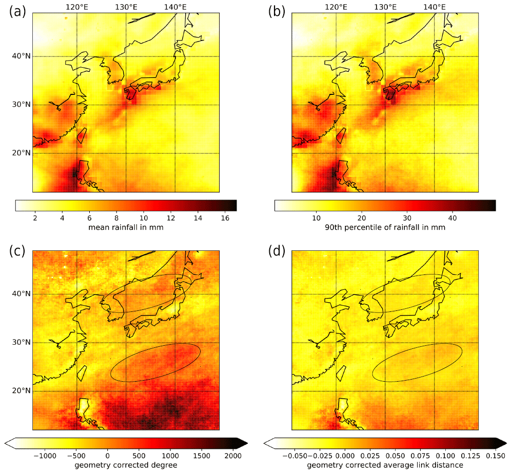
Figure 2 (a) Mean and (b) 90th percentile of daily rainfall sums between 25 April and 3 August over the study region. (c) Geometry-corrected degree and (d) average link distance of the climate network constructed based on synchronous occurrences of heavy rainfall events between 25 April and 3 August. The identified bands of elevated degree and average link distance are indicated by ellipses for better visual identification in panels (c) and (d).

It is important to not confuse the observed double-band structure with the concept of dipole structures known from empirical orthogonal function analysis of climate variability, which would normally correspond by definition to regions that exhibit negative correlations instead of varying in phase. Notably, correlation-based functional climate network approaches similar to that of the present work have also been used in the past for discovering previously overlooked dipole patterns in large-scale climate variability (Kawale et al., 2011), which is, however, distinctively different from what we attempt to achieve in the present work.

3.2 Monthly network patterns

In order to further study the temporal evolution of the network patterns uncovered above across the Baiu season and their connection with the intraseasonal dynamics of the EASM, we next examine the temporal evolution of the network structure over the full Baiu season. For this purpose, we compute the spatial patterns of degree and average link distance for the functional network representations obtained when evaluating the data for each calendar month separately. Hence, we obtain distinct networks for April, May, June, July, and August and show the resulting network patterns in Figs. 3 and 4. Specifically, the network characteristics of the main Baiu phase (May to July) are shown in Fig. 3, while those for the pre-Baiu (onset) and post-Baiu (withdrawal) phases (April and August, respectively) are shown in Fig. 4.

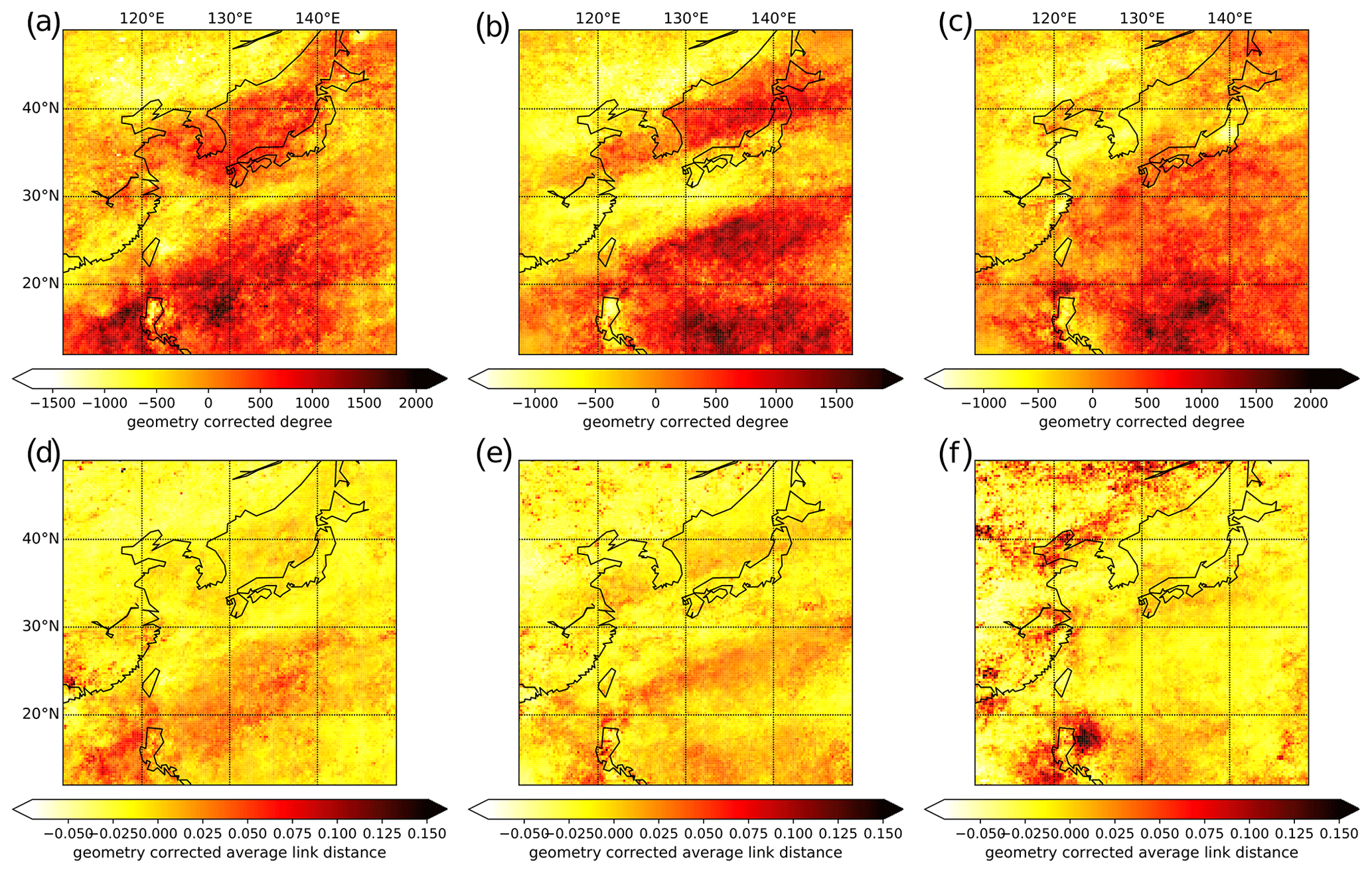
Figure 3 Network evolution during the active Baiu phase from May to July (left to right). Panels (a–c) show the degree patterns of the monthly networks, while panels (d–f) show the respective average link distance patterns.

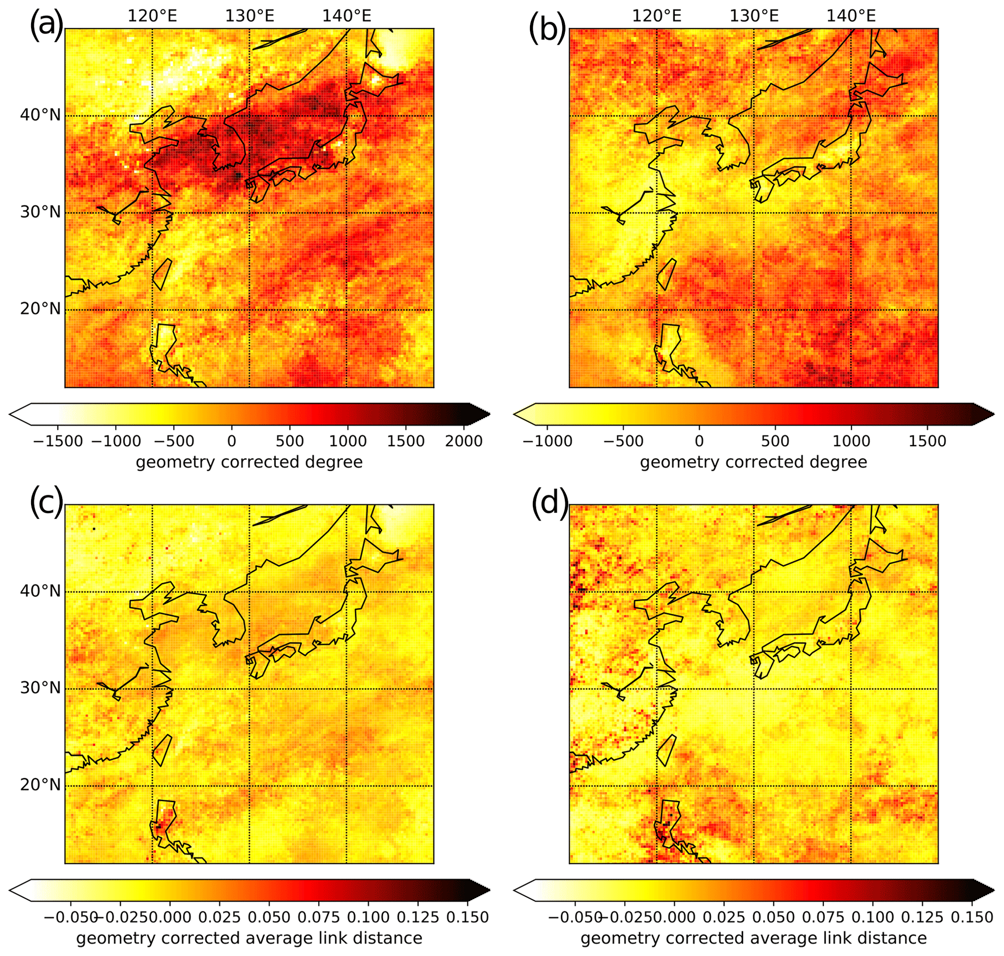
Figure 4 Network evolution before (April, a and c) and after (August, b and d) the active Baiu phase. (a, b) Geometry-corrected node degree and (c, d) average link distance.

The top panels in both figures show the node degree of the different networks and unveil dynamic changes over the EASM season. We confirm that the Baiu front is accompanied by a double-band structure of elevated degrees, with one band south of the front and another covering the Japanese Sea and the northern part of Honshu, which evolve over time and progressively migrate northward. This double-band structure, which is already visible in May in both degree and average link distance (Fig. 3a, d), is intimately related to the evolution of heavy rainfall associated with the Baiu front. In June, the corresponding pattern is most prominent (Fig. 3b, e), and a clear northward shift of the northern band is visible as compared to May. In addition, the degree maximum of the southern band migrates northwestward and exhibits a clearer band structure in the average link distance. This is in line with the development of the Baiu frontal system, which leads to the onset of the Baiu season over Honshu in early June. In July, the northern band with elevated degree is hardly recognizable anymore, while the southern band is further shifted northward, which is in good agreement with the further northward shift of the Baiu front in July (Fig. 3c). Interestingly, we observe a complete disappearance of the previously described link distance pattern (Fig. 3f). This observation is most likely caused by the disappearance of the northern high degree band and therefore the breakdown of the double-band structure (see Sect. 3.3 below). Whether this effect is exclusively caused by some dynamical reorganization of the regional atmospheric circulation or associated with some further northward shift of key patterns out of the study area cannot be further addressed in the context of the present work due to the spatial coverage of the TRMM data set exhibiting some northern boundary.

To capture the full evolution of the Baiu system, we also examine the pre- and post-Baiu phases by analyzing the patterns of degree and average link distance (Fig. 4). In April, we initially observe the double-band as a rather diffuse pattern in both degree and average link distance, with no clear separation between the different regions, which is in agreement with the Baiu onset at the beginning of May for the Okinawa region. Finally, in August, the previously described remaining pattern of elevated node degrees associated with the southern band vanishes as well and is replaced by different structures possibly more strongly affected by tropical cyclone tracks.

3.3 Evolution of the double-band structure

In an attempt to provide some climatological interpretation of the observed network structures, we next investigate the connectivity between the two observed high-degree bands and the role of the elevated average link distances in the respective regions. For this purpose, we first take a closer look at the community structure of the functional network representation covering a period between mid-June and mid-July. This period is chosen here because of the particularly strong double-band signature in June (see Fig. 3) and the fact that it corresponds to the most active phase of the Baiu developmental cycle over Japan (Ozturk et al., 2019). Hence, we expect to observe the clearest topological evidence for connectivity between the two bands in this period of the year – given that they are actually dynamically interconnected.

In Fig. 5a we show the community structure of the network that we obtain when we only analyze the time series segments starting from 14 June and covering a period of 30 d in each year, using the average symmetrization of the event coincidence rates. Notably, we again observe the double-band structure, where one community (colored in dark purple) is split into two spatially distinct parts, reflecting the two areas previously identified as the northern and southern bands in Fig. 3. From this result, we can conclude that the double-band structure in June and July is indeed related to synchronous rainfall activity in two spatially distinct regions, which implies the existence of long-distance dependencies between the two bands and suggests that both structures do not originate from two isolated mechanisms. In addition, we also observe other communities consisting of different parts (Fig. 5a), which indicates that during the peak Baiu phase, heavy rainfall also occurs synchronously between other spatially distinct regions. Since those regions are not characterized by outstanding values of node degree and average link distance in Fig. 3, we consider them here to be less climatologically relevant than the dark purple community representing our double-band pattern.

In order to further examine the general stability of the community pattern during the peak Baiu season, we have followed a cross-validation approach where five reduced data sets have been considered, each of which has 6 years of data missing (results not shown). In two out of the five cases, the community pattern looked almost indistinguishable from the one obtained for the full data set. In two other cases, the more southern community was shifted southward, larger, and separated from the northern one by an additional narrow community. Only one case did not exhibit a clear double-band community but instead two isolated communities representing comparable regions. Taken together, we conclude that the community structure provides some indication for the robustness of our double-band structure. In general, the concept of network communities is not uniquely defined, and it is known that community detection algorithms (including Infomap, which features some stochastic optimization components) tend to exhibit a certain degree of instability in their results. In this spirit, we take the findings from our cross-validation exercise as a strong indicator for qualitatively robust patterns.

While the previously described analyses of the community structures have solely focused on the peak Baiu season, we also consider the temporal evolution of long-distance connectivity associated with the identified double-band community during the entire EASM season. It can already be expected from the spatial precipitation patterns, which change dynamically along the season, that the obtained community structure is not stationary. To quantitatively trace the associated changes in the interconnectivity between the two regions forming the distinct parts of the double-band community during the peak Baiu phase, we define two characteristic regions largely overlapping with that community during mid-June to mid-July (white boxes in Fig. 5a). Then we pursue a sliding window approach by considering only corresponding time series segments of 30 d length from each year with observations, the starting date of which is successively shifted by one day from 1 April to 1 August. For each of the reduced data sets thus obtained, we generate a functional climate network representation as before, resulting in 123 different networks. For each of those networks, we compute the total cross-degree between the two selected regions, the values of which are shown in Fig. 5b.

Figure 5b reveals several features associated with the double-band structure. First, we observe a rapidly increasing total cross-degree between the two regions for time windows starting after 9 May in the case of the maximum symmetrization of the ECA, which exhibits a distinct maximum for windows starting around the mid of June. Second, we find a delayed increase of the total cross degree for the average symmetrization visible only for windows starting after 3 June, also peaking for time windows starting in mid-June. The second finding appears consistent with the mean onset date of the Baiu over Honshu. The earlier signal in case of the maximum symmetrization can be either related to the earlier onset of the Baiu in the region between Okinawa and Honshu or represents a direct precursor of the bidirectional synchronization of the heavy rainfall events developing in the course of the peak Baiu phase. Both aspects would suggest the existence of a physical mechanism that couples the respective regions in a time-dependent manner and thereby potentially affects the onset and progression of the Baiu season. The differences between the two different symmetrization approaches suggest that there is some kind of directed synchronization between the two regions after the onset of the Baiu in the Okinawa region, which gradually transforms into a more symmetric (bidirectional) one as soon as the Baiu-related coherent heavy rainfall activity hits Honshu island.

3.4 Inter-band synchrony of heavy rainfall events

From our initial analysis of the common climatological patterns, it already follows that most of the heavy rainfall associated with the Baiu front falls at the actual position of the front that typically lies above Kyushu and Honshu from mid-June to mid-July (Fig. 2a, b). This implies that the heavy rainfall events over the identified double-band structure do not necessarily correspond to the highest overall rainfall sums across the study area. In order to better understand the synchrony between heavy rainfall in the two bands, we now take a closer look at the situations corresponding to the synchronous heavy rainfall events in both bands.

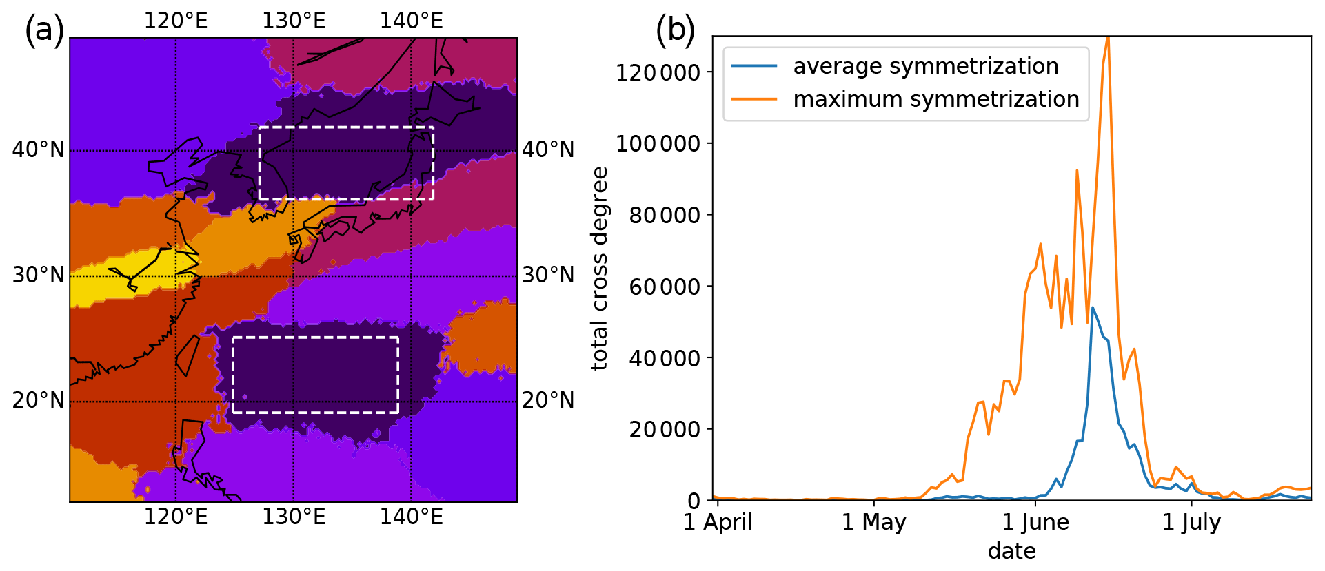
Figure 5 (a) Community structure of the network derived from heavy rainfall events between 14 June and 13 July of all years. (b) Total cross-degree between the regions marked by the white rectangles in (a) for 123 different networks computed from 30 d windows starting between 1 April and 1 August.

To identify those time periods that most likely dominate the specific signatures in the climate network properties described above, we consider the number of grid cells in the two previously defined regions of interest (Fig. 5a) for single days based on each 30 d window. This results in two new time series representing the respective numbers of events in both regions. From those event number series, we again consider the 90th percentile to define those days where the highest numbers of grid points synchronously exhibit heavy rainfall events. To tie in with the previous network analysis, we subsequently calculate the instantaneous event coincidence rate (with again ΔT=3 d) between the two event number time series for each of the 30 d windows used in the previous analysis. Similar to the results for the total cross degree between both regions studied in Sect. 3.3, this provides a time series of event coincidence rates for different windows, which is shown in Fig. 6a together with selected quantiles of a corresponding distribution of event coincidence rates drawn from random event sequences (1000 independent samples) with the same series length and number of events.

Figure 6a reveals two distinct phases of synchrony between spatially extended heavy rainfall activity in both regions of interest (high event coincidence rates) and one phase of effective anti-synchrony (extraordinary low event coincidence rate). Notably, the latter period of anti-synchrony does not coincide with a phase of high cross-degree in the network representation and indicates that during this phase spatially extended heavy rainfall in one region effectively suppresses (rather than promotes) corresponding events in the other and vice versa. This means that synchronous large-scale heavy rainfall events in both regions co-occur less frequently than expected for random sequences, motivating our use of the term anti-synchrony for describing both regions' behavior in the anti-phase according to the timing of heavy rainfall events. The corresponding finding might deserve special attention in future works but will not be further analyzed here since it corresponds to a time period that is likely more strongly affected by tropical cyclones than the developing and peak Baiu phase. Here, we are mainly interested in better understanding the constructive synchrony between both bands. Therefore, in what follows we will focus on the two corresponding periods, one associated with time windows starting at the beginning of April and the other coinciding with the period of elevated total cross-degree between both regions in the developed Baiu phase.

Figure 6 (a) Event coincidence rates between the days with the 10 % most synchronous events in both regions of interest (Fig. 5a) for the same sliding windows as in Fig. 5b. Different shadings represent the corresponding quantiles (0.1, 0.25, 0.75, 0.9) estimated from 1000 surrogate event sequences constructed from the underlying ones by random shuffling of the events.(b, c) Rainfall composites for those days on which the number of heavy rainfall events exceeds its empirical 90th percentile in both regions during the periods (b) 4 April–3 May and (c) 14 June–13 July, respectively.

Table 1 Days with high numbers of grid cells exhibiting heavy precipitation events in the two regions of interest during phase 1 (4 April–3 May, left) and phase 2 (14 June–13 July, right) that have been used for defining the composites shown in Fig. 6b and c, respectively. The numbers of grid points in the two regions of interest (and therefore the maximum possible number of grid points with events per day) are 1375 for the northern region and 1344 for the southern region, respectively.

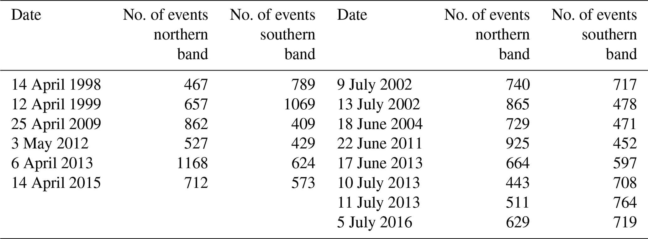
To illustrate the key mechanisms leading to widespread simultaneous heavy rainfall events in both regions, we show composites of daily rainfall sums from days with particularly high “activity” in both regions during both periods (event coincidence rates exceeding the corresponding 75th percentile) in Fig. 6b, c. Both panels focus on those days for which we observe heavy rainfall events occurring simultaneously in both regions, which are listed in Table 1. Specifically, only those days are used here at which the number of grid points with heavy rainfall events exceeds their respective 90th percentile simultaneously in both regions. Although both composites are therefore based on data from a few days only (phase 1: 6 days; phase 2: 8 days), we observe some distinct climatic patterns leading to the elevated event coincidence rates. In phase 1 (Fig. 6b), which is particularly prominent in the 30 d period starting 4 April, heavy rainfall is caused by a major large-scale weather system extending over both regions and the area between them. In phase 2 (Fig. 6c), which coincides with the fully developed Baiu phase over Kyushu and Honshu, we instead observe two spatially separated systems with heavy rainfall (here shown for the time window starting on 14 June). Only the latter configuration is characterized by an elevated cross-degree, since both contiguous heavy rainfall patterns fully fall into the separated regions, while other areas are far less affected by heavy rainfall, which is the major difference to the configuration in phase 1. This result is representative for other time windows with elevated event coincidence rates (not shown).

4 Discussion

4.1 Climatological controls on Baiu dynamics

The results of the network analysis presented in Sect. 3 have been solely based on heavy rainfall events in the considered study area. In order to link the observed spatio-temporal patterns of synchronous heavy precipitation with large-scale atmospheric processes that are more directly reflected by other climate variables, we take an additional look at the associated geopotential height, relative vorticity, and high altitude and low-level wind fields in terms of their mean climatology across the EASM spatial domain and season.

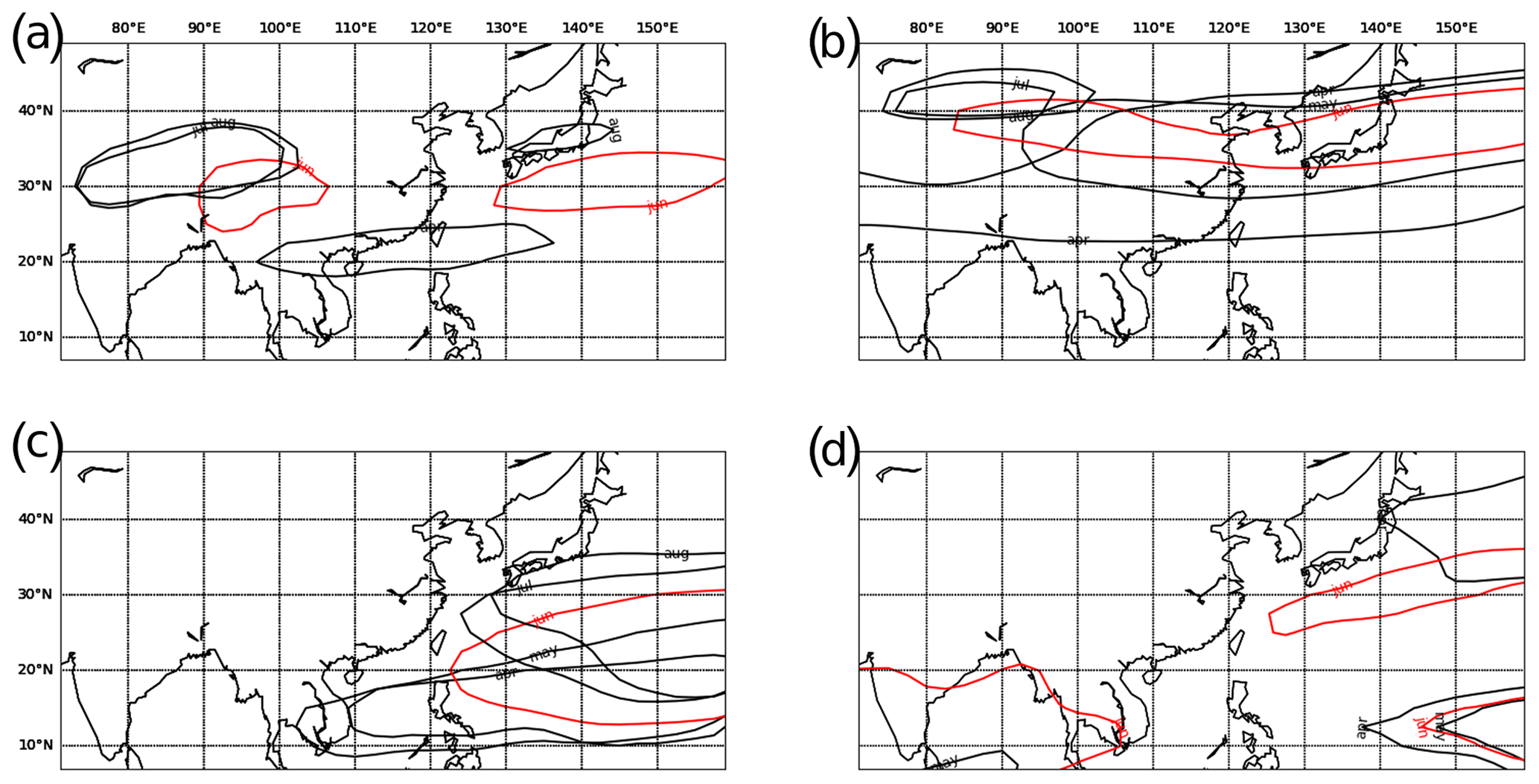
Figure 7 Monthly mean contour of (a) 200 hPa relative vorticity at $\mathrm{2.8}\times {\mathrm{10}}^{-\mathrm{5}}{\text{s}}^{-\mathrm{1}}$, (b) 200 hPa isotachs of 30 ms⁻¹, (c) 500 hPa geopotential height at 5880 m, and (d) 850 hPa isotachs of 7 ms⁻¹ during April–August. Contours in June are colored red.

The development of the Baiu front and associated rainfall is widely known to have a close relationship with the EASM (Chen, 1994). While Baiu is often associated with the frontal development over southern China (as Meiyu) and Taiwan, the Baiu onset time usually coincides with that of the EASM. Moreover, the active Baiu season with intense rainfall is associated with increased moisture transport by southwesterlies in the EASM domain. Several studies have also revealed that the formation of the Baiu front over the Yangtze River valley region in China, as well as Japan, is correlated with the onset of the ISM and have demonstrated that at both intraseasonal and interannual timescales, the precipitation in Kerala, India (commonly used for defining ISM onset), is significantly correlated with that in the Baiu region through the so-called southern mode of teleconnection (Krishnan and Sugi, 2001; Liu and Ding, 2008; Li et al., 2018).

In the context of this teleconnection mode, the South Asian Anticyclone (SAA) plays an important role. Li et al. (2018) indicate that the intensity of the SAA is correlated with the upper-level jet from the Tibetan plateau to the Baiu region, which is known as a favorable factor for the frontal development. Climatologically, the upper-level relative vorticity during April and May is weak over South Asia and East Asia. The SAA first appears in June and further extends during July and August (identified as relative vorticity of the order of $\mathrm{3}\times {\mathrm{10}}^{-\mathrm{5}}{\text{s}}^{-\mathrm{1}}$, see Fig. 7a). The SAA is also part of the zonally oriented upper-level wave train of a cyclone–anticyclone–cyclone pattern identified in the study of Krishnan and Sugi (2001). The cyclone to its east is responsible for the mid-level jet into the Baiu region. When the SAA develops during June the mid-level jet extends from the SAA to the Baiu development region through a latitudinal band at about 35 to 40^∘N, which is remarkably narrow when compared with that in April and May (Fig. 7b). During July and August, this jet retreats to the west. Interestingly, Li et al. (2018) also demonstrated that an intense SAA is consistent with a strong upper-level meridional temperature gradient over southern Japan, which may be related to the midlevel temperature advection during early June reported by Okada and Yamazaki (2012) and the large meridional temperature gradient analyzed in Tomita et al. (2011).

Also relevant to the Baiu development but commonly considered independent of the SAA (correlation coefficient of 0.02 estimated by Li et al., 2018) is the Northwest Pacific Subtropical High (NPSH). At higher altitudes, the NPSH is characterized by a stable low-pressure system that provides the strong upper-level westerly jet south of Japan. The westerlies north of the ridge of the NPSH reach down to the low levels at about the same latitudes (Liu and Ding, 2008) and thereby provide the pre-frontal winds for the Baiu development. Climatologically, the NPSH develops at higher latitudes outside the tropics during June (Fig. 7c). During that month, the northern boundary of the NPSH is at about 30^∘ N and thus the westerlies north of the ridge are located just south of Japan. During July and August, the average ridge expands further to the north, which is consistent with the northward migration of the Baiu front. Compared with the pre-Baiu period of April–May, it is also only in June that the strong westerly belt associated with the NPSH extends from the position of the NPSH in the Pacific Ocean to almost the western coast of the Pacific near Taiwan (Fig. 7d), which provides a favorable wind structure for frontal development.

Considering all observations mentioned above, we suspect that the north–south double-band structure as clearly depicted in the network measures of node degree and average link distance especially during June is a representation of two previously assumed independent factors responsible for the Baiu development: the SAA as part of the coupled ISM and EASM system, and the NPSH that develops over the Pacific Ocean. The synchrony between heavy precipitation events likely controlled by both mechanisms therefore indicates a dynamical coupling between SAA and NPSH that has not been described previously to the best of our best knowledge. We emphasize, however, that our analysis has focused on specific events, while previous work on Baiu dynamics and related phenomena has almost exclusively utilized standard (linear) analysis techniques based on correlations or composites commonly applied to other atmospheric variables (among other reasons, a statistically rigorous evaluation of correlations for daily precipitation data is complicated by the commonly large number of zeros; cf. Ciemer et al., 2018). Therefore, it is possible that the hypothesized coupling might not act persistently but rather intermittently during specific large-scale synoptic situations. A more in-depth investigation on this aspect is outlined as a subject of future research.

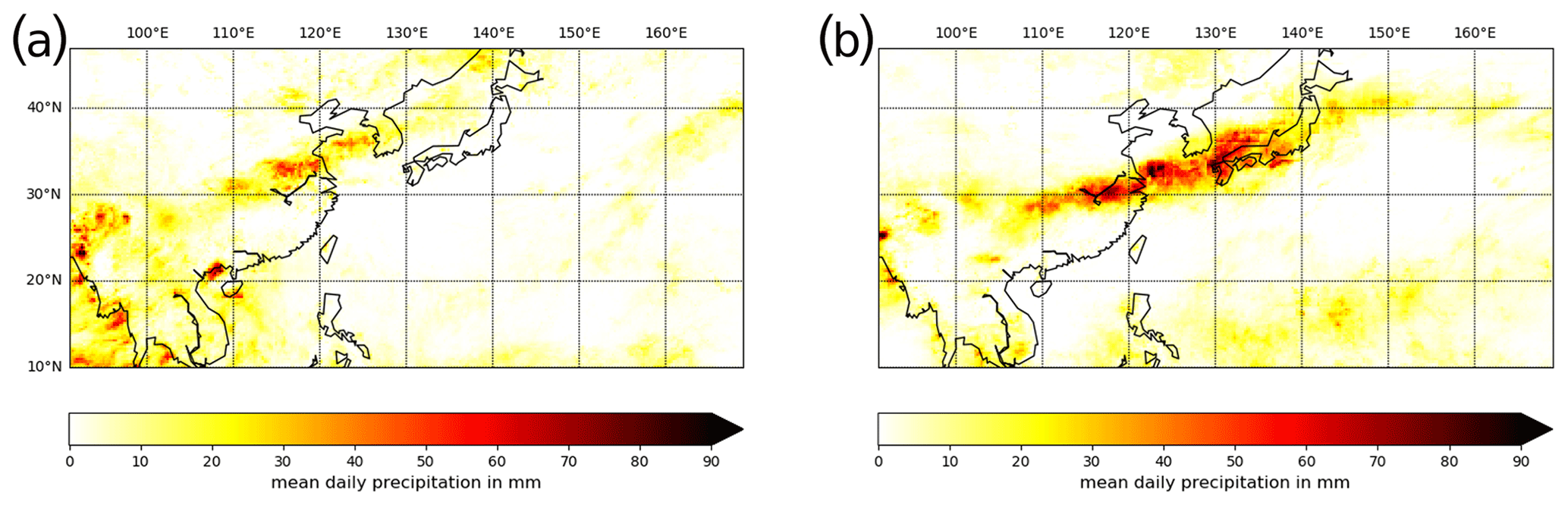
Figure 8 Mean daily precipitation (a) between 29 June and 3 July 1998 and (b) between 25 and 30 June 1999.

4.2 Illustrative examples: 29 June–3 July 1998 and 25–30 June 1999

To further illustrate the atmospheric processes associated with Baiu development, two cases previously analyzed by Guan et al. (2020) are considered in more detail. Guan et al. (2020) termed the southwest-to-northeast development of the Baiu front as a corridor of rainfall. Interestingly, they also identified a double-band structure of synoptic factors facilitating the development of severe rainfall at the front. The first two years of our study period (1998–1999) are among the particularly active Baiu years and clearly highlight the driving synoptic processes. For example, during the period between 29 June and 3 July 1998, it can be seen that severe rainfall occurred in the Bay of Bengal and extended to northeastern China through the frontal rainfall band (Fig. 8a). Between 25 June and 30 June 1999, the Baiu rain band extended more to the east and covered substantial parts of Kyushu and Honshu (Fig. 8b).

The double-band structure found by Guan et al. (2020) consists of a north–south pair of anticyclone and cyclone at low level, which the authors referred to as the Tropical Anomalous Anticyclone (TAAC) and the Midlatitude Anomalous Cyclone (MAC), respectively. From their interannual variability analysis, it is evident that the MAC–TAAC pair was strongly developed in June 1998 (Fig. 9a) with strong southwesterlies driving the cyclonic flow to the north. The anticyclone in the south originated from the NPSH shown in Fig. 7. Associated with this double-band, there was a significant meridional gradient of geopotential height (Fig. 9b). At the same time, the upper-level jet with wind speed over 35 m s⁻¹ was driving the convection at the frontal surface.

As opposed to the former case, in the event of June 1999, the TAAC was similar to the year before, while the MAC was not as strong (Fig. 9c). In addition to the dynamic factors, moisture-related processes are important to organize the convection at the frontal surface. In the case of 1999, moisture was abundant in vast areas in eastern South Asia. Along the southwesterlies extending from the northern side of the NPSH (or TAAC), an updraft existed in the low-level to midlevel areas, which is a key dynamic factor for organizing convection (Tan et al., 2015). Considering the main moisture source is located over southern Asia, advection is the major process to transport the moisture into the frontal zone, with a weak convergence flow over southern Japan enhancing the convection at the front (Fig. 9d). In comparison with the frontal rain bands in Fig. 8, it is evident that the moisture transport by the southwesterlies associated with the MAC enhances the convection at the Baiu front. To the south, since the TAAC is associated with a high-pressure system, rainfall has been suppressed over that region. Nevertheless, the southern band in our network analysis has revealed strong synchrony of heavy rainfall there, likely due to a control by the TAAC.

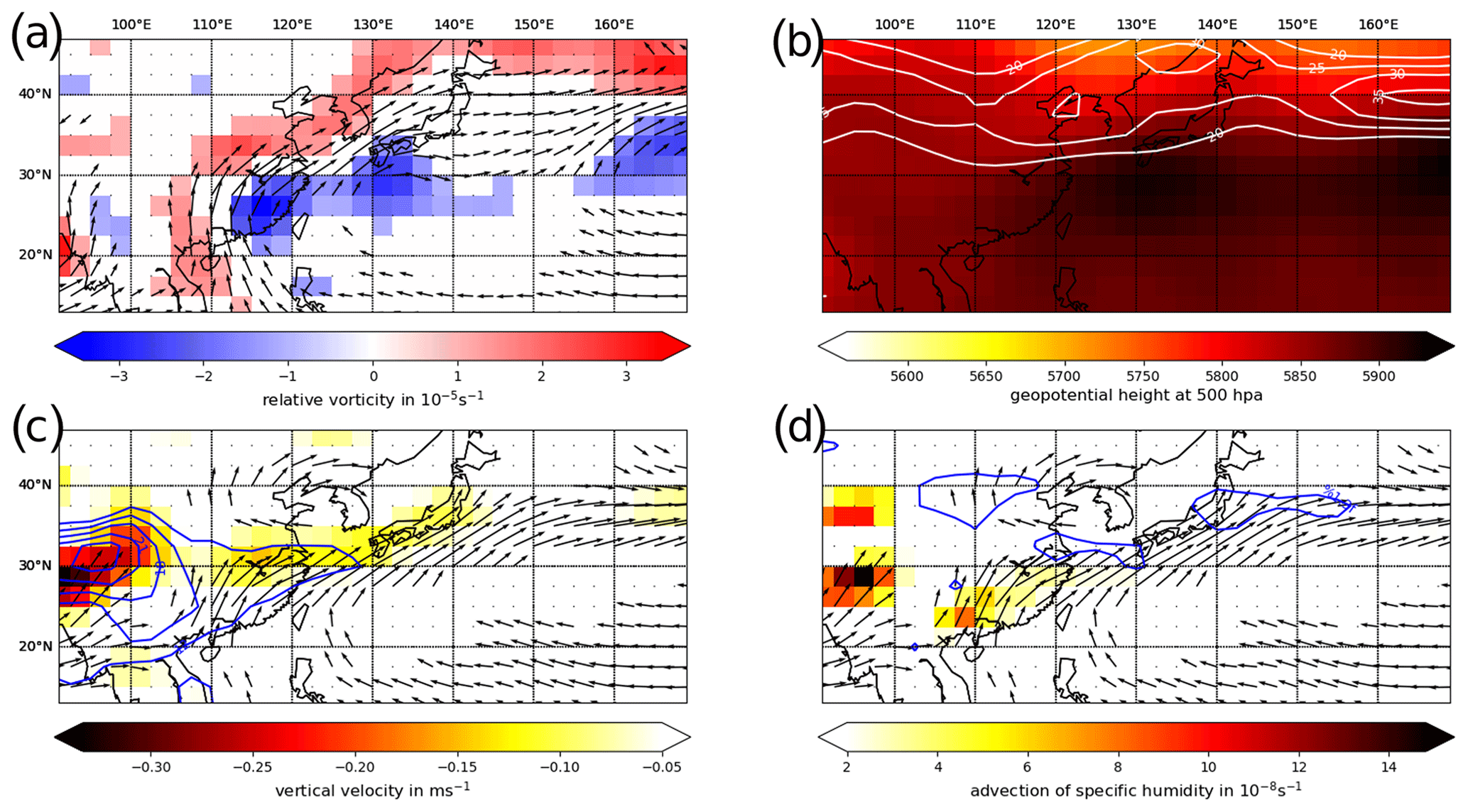
Figure 9 (a) Average (29 June–3 July 1998) 850 hPa winds with speed larger than 5 m s⁻¹ and relative vorticity larger than 10⁻⁵ s⁻¹ (red tones) and smaller than $-{\mathrm{10}}^{-\mathrm{5}}$ s⁻¹ (blue tones). (b) Average (29 June–3 July 1998) 500 hPa geopotential height (shaded) and 200 hPa wind speed larger than 20 m s⁻¹ (white contours). (c) Average (25–30 June 1999) 850 hPa winds with speeds larger than 5 m s⁻¹, specific humidity larger than 12 g kg⁻¹ (blue contour, interval 3 g kg⁻¹) and 700 hPa updraft vertical velocity larger than 0.05 Pa s⁻¹ (shaded). (d) Winds are the same as in (c) but are combined with specific humidity advection larger than $\mathrm{2}\times {\mathrm{10}}^{-\mathrm{8}}$ s⁻¹ (shaded) and divergence at −0.01 m s⁻¹ (i.e., convergence, blue contour).

4.3 Synoptic patterns of days with strong inter-band activity

To further clarify the formation of the double-band structure in the climate network, we study composites of different climatological variables (Fig. 10) corresponding to the same days (see Table 1) as used for the rainfall composites in Fig. 6c, which are closely connected to the elevated cross-degree in the network in the period from mid-June to mid-July.

The relative vorticity (Fig. 10a) highlights the role of the NPSH (blue shading) and the corresponding clockwise rotating low-level winds, leading to the rainfall associated with the southern band. The NPSH-related elevated values of geopotential height are depicted in Fig. 10b together with the 200 hPa wind speed, showing the SAA-related jet closely associated with the northern rainfall band in the Japanese Sea.

Matching with the two regions of spatially coherent distant rainfall, we observe two spatially separated regions of strong updraft, which appear to be connected by the mentioned low-level winds (see Fig. 10c). To investigate the updraft-induced cloud formation, we also show the outgoing longwave radiation (OLR) anomalies in Fig. 10d. The pattern shown by the OLR anomaly during the selected days is very similar to that of the rainfall composite in Fig. 6c, as well as the network measures, and shows negative values connected with enhanced cloud formation in both regions that are linked in the network. Specifically, the southern band is characterized by very low OLR values, which provides an indication for tropical deep convection, while the generally somewhat larger values in the northern band indicate that the convective rainfall in this region instead originates from extratropical processes.

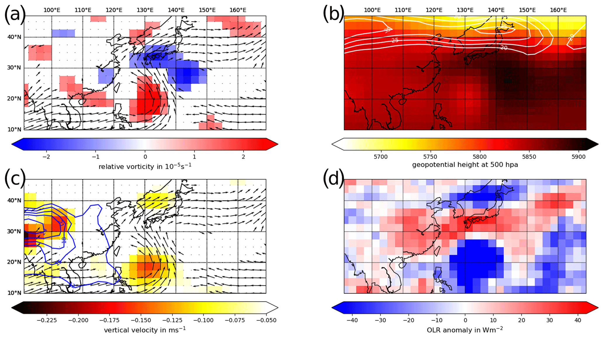
Figure 10 Composites based on the dates with strong inter-band activity (see Fig. 6c and Table 1). (a) Average 850 hPa winds with speed larger than 5 m s⁻¹ and relative vorticity larger than 10⁻⁵ s⁻¹ (red tones) and smaller than $-{\mathrm{10}}^{-\mathrm{5}}$ s⁻¹ (blue tones). (b) Average 500 hPa geopotential height (shaded) and 200 hPa wind speed larger than 20 m s⁻¹ (white contours). (c) Average 850 hPa winds with speed larger than 5 m s⁻¹, specific humidity larger than 12 g kg⁻¹ (blue contour, interval 3 g kg⁻¹) and 700 hPa updraft vertical velocity larger than 0.05 Pa s⁻¹ (shaded). (d) OLR anomalies with respect to the NOAA long-term mean between 1981–2010.

4.4 Insights and perspectives of network analysis

Utilizing our network analysis, we have identified a double-band structure of synchronous heavy rainfall events along the Baiu frontal zone, with the northern band most likely resulting from the upper-level jet originating from the SAA and the southern band representing the low-level jet emanating from the NPSH. Both bands form a single network community persisting during the active Baiu phase (Fig. 5), which demonstrates that the two major (but commonly considered independent) synoptic factors for Baiu development are intimately linked as manifested in the single system variable heavy rainfall. In other words, during Baiu development the heaviest rainfall events north and south of the front are synchronized with a spatial pattern that is distinct in its characteristics as compared to the pre- and post-Baiu periods. This suggests a potential mechanism that could provide a novel approach for developing a predictor scheme for Baiu onset based on network measures, which should be further explored in future studies.

For a dynamical model-based prediction of the onset dates of Baiu but also the closely associated ISM onset dates (Liu and Ding, 2008; Li et al., 2018), the ability of a model to simulate the SAA and the NPSH over the Pacific (and likely also the associated mesoscale convective systems) would affect the prediction skill. The observed double-band structure associated with heavy rainfall north and south of the Baiu front, which to our best knowledge has not been described before, could aid evaluating such dynamical models. Moreover, the mechanism for its generation as discussed above could be further exploited to provide a potential predictor for improved statistical forecasting schemes. Notably, a predictor considering the synchrony revealed by the community structure would complement any prediction based on ISM or SAA alone because the largest community identified by our network analysis comprises the synoptic influence from the Pacific Ocean as well. Although evidence has to be further identified, many years in which the onset date of Baiu was quite different from that of the ISM have been El Niño years (Liu and Ding, 2008). Thus, processes from the Pacific Ocean likely constitute critical factors for Baiu development. Nonetheless, only the mean seasonal evolution of the Baiu has been analyzed in this study, and therefore the presented methodology should be further extended to be able to analyze interannual variability before any improvement on Baiu prediction can be attempted.

5 Conclusions and outlook

In this study, we have investigated the temporal evolution of heavy rainfall patterns related to the East Asian summer monsoon (EASM). Specifically, we have investigated the timing of heavy rainfall events across the monsoon season by utilizing functional climate networks along with event coincidence analysis and have found a previously not reported double-band structure of two spatially distinct regions with synchronous heavy rainfall, the emergence of which appears intimately linked with the onset of the Baiu over Japan.

To extend previous static network-based analyses of Baiu-related rainfall (Ozturk et al., 2018, 2019), we have studied the evolution of heavy rainfall event-based synchrony patterns over time by utilizing a sliding window approach. For time windows of 30 d successively shifted over the period of the EASM from April to August, we have constructed functional climate networks and have characterized the formation and breakdown of a double-band structure, which is visible from the beginning of May to the end of July in the node degree and average link distance patterns of the respective networks. In addition, we have shown that the interconnectivity between the two distinct regions forming this double-band emerges in a complex manner, which is characterized by a directional synchrony pattern emerging with the beginning of the Baiu season in the Okinawa region (mid-May) that tends to develop into a bidirectional relationship at about the time when the Baiu front hits Honshu island in June. We have confirmed this finding by investigating the community structure of the network and have shown that the double-band is, during the peak Baiu phase, indeed represented by a unique spatially split community consisting of two distinct contiguous regions synchronously experiencing heavy rainfall.

We have further shown that the northern band is related to the upper-level jet triggered by the South Asian Anticyclone while the southern band emerges due to the low-level jet resulting from the Northwestern Pacific Subtropical High. As our network analysis has revealed the bidirectional dependence of heavy rainfall related to the two different drivers and that the associated temporal evolution is intimately connected with the onset of the Baiu, we suggest that our findings can contribute to future developments of complementary predictors of Baiu onset based on the identified event synchrony patterns.

Finally, we emphasize that our synoptic analysis has linked the observed double-band structure to two different drivers that have been previously assumed to serve as independent actors in East Asian summer monsoon dynamics. The observation that two associated outstanding regions north and south of the Baiu front are characterized by synchronous heavy rainfall activity may have two possible explanations: either a common driver behind the corresponding processes controlling precipitation dynamics in both regions or a previously disregarded mutual coupling between their respective drivers. In order to reject either of these two possible hypotheses, the more qualitative synoptic analysis performed here needs to be further extended into a quantitative one, going beyond a purely correlative study by explicitly accounting for possible directional cause–effect relationships. Corresponding follow-up investigations using novel tools of statistical climatology like causal effect networks or response-guided causal precursor detection (Runge et al., 2015; Kretschmer et al., 2016; Di Capua et al., 2020) are therefore outlined as relevant topics for future work.