the Creative Commons Attribution 4.0 License.
the Creative Commons Attribution 4.0 License.
 | 15 Oct 2021
Vulnerability of European ecosystems to two compound dry and hot summers in 2018 and 2019
René Orth
Markus Reichstein
Philippe Ciais
Nicolas Viovy
Sönke Zaehle
Peter Anthoni
Almut Arneth
Pierre Gentine
Emilie Joetzjer
Sebastian Lienert
Tammas Loughran
Patrick C. McGuire
Sungmin O
Julia Pongratz
Stephen Sitch
In 2018 and 2019, central Europe was affected by two consecutive extreme dry and hot summers (DH18 and DH19). The DH18 event had severe impacts on ecosystems and likely affected vegetation activity in the subsequent year, for example through depletion of carbon reserves or damage from drought. Such legacies from drought and heat stress can further increase vegetation susceptibility to additional hazards. Temporally compound extremes such as DH18 and DH19 can, therefore, result in an amplification of impacts due to preconditioning effects of past disturbance legacies.
Here, we evaluate how these two consecutive extreme summers impacted ecosystems in central Europe and how the vegetation responses to the first compound event (DH18) modulated the impacts of the second (DH19). To quantify changes in vegetation vulnerability to each compound event, we first train a set of statistical models for the period 2001–2017, which are then used to predict the impacts of DH18 and DH19 on enhanced vegetation index (EVI) anomalies from MODIS. These estimates correspond to expected EVI anomalies in DH18 and DH19 based on past sensitivity to climate. Large departures from the predicted values can indicate changes in vulnerability to dry and hot conditions and be used to identify modulating effects by vegetation activity and composition or other environmental factors on observed impacts.
We find two regions in which the impacts of the two compound dry and hot (DH) events were significantly stronger than those expected based on previous climate–vegetation relationships. One region, largely dominated by grasslands and crops, showed much stronger impacts than expected in both DH events due to an amplification of their sensitivity to heat and drought, possibly linked to changing background CO2 and temperature conditions. A second region, dominated by forests and grasslands, showed browning from DH18 to DH19, even though dry and hot conditions were partly alleviated in 2019. This browning trajectory was mainly explained by the preconditioning role of DH18 on the impacts of DH19 due to interannual legacy effects and possibly by increased susceptibility to biotic disturbances, which are also promoted by warm conditions.
Dry and hot summers are expected to become more frequent in the coming decades, posing a major threat to the stability of European forests. We show that state-of-the-art process-based models could not represent the decline in response to DH19 because they missed the interannual legacy effects from DH18 impacts. These gaps may result in an overestimation of the resilience and stability of temperate ecosystems in future model projections.
- Article
(19017 KB) - Full-text XML
- BibTeX
- EndNote


Extreme dry and hot summers in western and central Europe have become more frequent over the past decades (Coumou and Rahmstorf, 2012; Seneviratne et al., 2014), a trend that is expected to continue as global mean temperatures rise (Barriopedro et al., 2011). Hot extremes in Europe are promoted by changes in atmospheric circulation (Coumou et al., 2015; Drouard et al., 2019) and amplified by strong feedbacks between the land surface and the atmosphere, being therefore also associated with severe droughts (Miralles et al., 2014; Samaniego et al., 2018), i.e. compound dry and hot events (DH).
In Europe, DH events usually have strong negative impacts on ecosystems, such as reduced ecosystem productivity (Ciais et al., 2005; Bastos et al., 2020b). After severe drought and heat stress, plant recovery can be lagged, for example due to reduced growth or non-reversible losses in hydraulic conductance or carbon reserve depletion (Ruehr et al., 2019). This in turn may increase vulnerability to another DH if it occurs before complete recovery. Repeated droughts have been linked to increased forest vulnerability in the northern mid-latitudes, albeit with variable responses (Anderegg et al., 2020). Impaired functioning during the recovery period can additionally increase the hazard of subsequent disturbances, e.g. insect outbreaks (Rouault et al., 2006). However, reductions in leaf area, increases in root allocation (McDowell et al., 2008), or reduced growth, caused by reducing evaporative tissue and enhancing water uptake capacity, could also confer an advantage to subsequent droughts (Gessler et al., 2020). It remains unclear whether the increased vulnerability to a subsequent drought can be explained by compounding hazards (e.g. accumulated water deficits or compound heat) or modulating effects due to vegetation responses to the first event.
In Europe, the summer of 2018 was the hottest since 1500 (Sousa et al., 2020) and associated with an unprecedented area affected by drought (Albergel et al., 2019; Bastos et al., 2020a). This DH event resulted in decreases in ecosystem productivity by up to 50 % in central Europe (Bastos et al., 2020a; Buras et al., 2020) and crop yield losses (Beillouin et al., 2020). Part of the central European region affected by the dry and hot summer in 2018 registered another extremely hot and dry summer in 2019 (Boergens et al., 2020; Sousa et al., 2020).
From a hydrometeorological perspective, each of the dry and hot summers in 2018 and 2019 (DH18 and DH19, respectively) can be considered a multivariate compound event in that both high temperatures and strong drought conditions were observed (Zscheischler and Fischer, 2020). Taken together, they can be considered a temporally compound event (Zscheischler et al., 2020). For example, Boergens et al. (2020) have shown that while soil moisture deficits in summer 2019 were not as pronounced as in 2018, total water storage was lower in 2019 due to the water storage deficit resulting from the 2018 event. Given the unprecedented magnitude of DH18, it is likely that at least some ecosystems had not yet fully recovered in 2019. Therefore, from an ecological perspective, DH19 could additionally be considered a preconditioned compound event, where the impact of DH18 may affect the response to DH19 (Fig. 1). Finally, vulnerability to DH events can be further modulated by long-term environmental changes: water savings from reduced stomatal conductance should attenuate drought stress (Peters et al., 2018), but a concurrent decrease in evapotranspirative cooling along with “hotter droughts” may amplify heat stress (Allen et al., 2015; Obermeier et al., 2018).
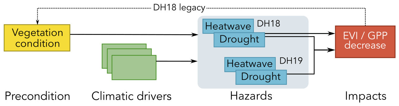
Figure 1Conceptual description of the compound DH18 and DH19 events. Dry and hot conditions in both summers were a result of compounding atmospheric drivers (synoptic patterns, preceding climate anomalies, land–atmosphere interactions). The DH18 impacts were preconditioned by seasonal legacy effects in ecosystem functioning from a sunny and warm spring. We hypothesise that legacies from the DH18 event also acted as a precondition of the response to DH19. Further modulating effects (not shown) include impacts of anthropogenic climate change on drivers, hazards, vegetation conditions, and land cover in modulating responses to hazards.
Separating the modulating effects controlled by vegetation responses to global change or by legacies from past disturbances (Kannenberg et al., 2020) and seasonal legacy effects (Buermann et al., 2018) in observations is problematic as it requires considering the compounding effects of multiple drivers (e.g. synergistic effects of heat and drought stress) and separating the role of seasonal and inter-annual legacies both in physical variables (e.g. soil-moisture depletion) and in vegetation vulnerability to those drivers. This can be done by designing counterfactual scenarios to force process-based models, as has recently been done to evaluate seasonal legacy effects of hot and dry springs (Lian et al., 2020; Bastos et al., 2020a). However, it has been argued that Earth system models fail at modelling woody biomass trajectories following droughts (Anderegg et al., 2015), and thus they might miss inter-annual legacy effects from DH events, although no simulations designed to isolate the individual impact of drought over subsequent years have been performed. Alternatively, statistical models can be used to separate such effects based on observational data (Chan et al., 2021).
Using both remote sensing data and an update to the simulations by Bastos et al. (2020a), we attempt to separate these different effects, namely how the combination of hot and dry conditions affected the vulnerability of ecosystems to the two events (multivariate compound event), how the repetition of a dry and hot summer affected the response to DH19 (temporally compound event), and how inter-annual legacy effects due to impacts of DH18 affected ecosystem vulnerability to DH19 (preconditioned compound event). We first use a statistical modelling approach to evaluate whether signs of increased vegetation vulnerability to DH18 and DH19 can be found and to attribute changes in vulnerability to inter-annual legacies and other modulating effects. We then compare observation-based results to updated simulations by state-of-the-art land surface models and dynamic global vegetation models (for simplicity referred to as LSMs) designed to isolate the impacts of DH18 and their legacy effects (Bastos et al., 2020a).
2.1 Climate variables
In ecological studies, drought is better characterised by soil moisture anomalies i.e. agricultural drought (Sherriff et al., 2011; Seneviratne et al., 2012; Samaniego et al., 2018), than atmospheric drought indices. We therefore base our drought assessment on two complementary soil moisture datasets. The first is the observation-based soil moisture dataset obtained from SoMo.ml (Sungmin and Orth, 2021), used as reference in this study, and the second, for comparison with SoMo.ml, is given by ERA5 volumetric soil water content (Hersbach et al., 2020).
The SoMo.ml data are generated using a long short-term memory neural network model trained with meteorological forcing from ERA5 and land surface characteristics as inputs and global in situ soil moisture measurements (Dorigo et al., 2011; Zeri et al., 2020) as target variables. The data cover soil moisture in the first 50 cm of the soil and are available at 0.25∘ lat/long resolution and daily time steps for the period 2000–2019. We remapped the fields to the finer resolution of the MODIS grid and aggregated the data to monthly means. We then subtracted the mean seasonal cycle and long-term linear trend and divided this by the corresponding standard deviation to obtain standardised soil moisture anomalies (SManom).
Monthly temperature and volumetric soil water content from the ECMWF ERA5 Reanalysis were obtained from the Copernicus Climate Change Service at 0.25∘ lat/long resolution (Hersbach et al., 2020) at monthly time steps, selected for the period 2000–2019 (common with SoMo.ml), and remapped to the finer resolution of the MODIS grid using conservative remapping. Standardised anomalies were calculated as described for SManom for ERA5 temperature and soil moisture fields (Tanom, ). Soil moisture anomalies from ERA5 in layers 1–2 (top 28 cm) are used for comparison of drought conditions with those estimated by SoMo.ml, although the two datasets are not fully independent.
2.2 Vegetation and soil data
We used the 16 d enhanced vegetation index (EVI) from the Moderate Resolution Imaging Spectroradiometer (MODIS) sensor from the MOD13C1 Climate Modeling Grid (CMG) product. The MOD13C1 CMG provides continuous cloud-free spatial composites from 1 km data projected on a 0.05∘ lat/long grid (Didan et al., 2015) and was selected for the period 2001–2019. Standardised EVI anomalies (EVIanom) were calculated following the same approach as for climate variables. The standardisation allows comparing the relative magnitude of anomalies for pixels with distinct temporal variability patterns and with vegetation productivity simulated by LSMs, which have different physical units.
We used land cover distribution in 2018 from the ESA Climate Change Initiative land cover (Kirches et al., 2014) (CCI-LC). The data are originally provided in land cover classes at 300 m spatial resolution and were converted to fractional cover at 0.05∘ lat/long resolution for forest, grassland, and crop classes using the CCI-LC user tool.
We used isohydricity fields from global satellite measurements from Konings et al. (2017) at 1∘ lat/long resolution. Anisohydric plants (low isohydricity) show weak regulation of stomatal opening and prioritise carbon assimilation over water savings during droughts. High isohydric plants show strong stomatal regulation of productivity and thereby preserve water at the cost of carbon assimilation during drought.
We use soil available water capacity (AWC) from Ballabio et al. (2016) and Panagos et al. (2012), which used the Land Use and Cover Area frame Statistical survey (LUCAS) topsoil database to map soil properties at continental scale.
2.3 Outputs from land surface and global dynamic vegetation models
Standardised anomalies of gross primary productivity (GPPanom) and soil moisture (SManom) were estimated by the mean of seven land surface models and dynamic global vegetation models (for simplicity referred to as LSMs) between 1979–2019 from an extension of Bastos et al. (2020a) simulations: a baseline simulation for comparison with observations and a factorial simulation to quantify the individual impact of summer 2018 and its legacy effects, when compared to the reference simulation. A detailed description of the models used and the simulation protocol is provided in Appendix A.
First, all model outputs were remapped to a common 0.25∘ grid, and the multi-model ensemble mean was calculated for the common period with MODIS (2001–2019). The variables were then deseasonalised, detrended, and standardised as was done for the other variables in the study.
3.1 Drought characterisation
We use the observation-based SoMo.ml as a reference dataset to define agricultural drought conditions. Regions with average SManom below −1σ (Seneviratne et al., 2012) during summer (June, July, and August, JJA) are considered drought-affected areas during the DH events. Then, a regional domain affected by both DH18 and DH19 events is selected to evaluate the impacts of two consecutive DH events. Within this region most pixels had negative SManom and the majority registered , but they differ in the magnitude of agricultural drought in DH19. This allows for comparing responses across pixels for different combinations of stress between DH18 and DH19. Since we are interested in evaluating how recovery from DH18 affected impacts of DH19, we limit our analysis to pixels with negative EVIanom in DH18.
3.2 Compound DH18 and DH19 events
3.2.1 DH18 and DH19 impact characterisation
To characterise different response types to DH18 and DH19, we group pixels using unsupervised clustering of EVI during the two extreme summers. Using an unsupervised method allows for avoiding making assumptions about the magnitude of impacts or the trajectory between DH18 and DH19 (DH18 → DH19) when grouping pixels. For this, we applied a k-means cluster analysis (Hamerly and Elkan, 2003) using two features, corresponding to the EVIanom fields in DH18 and DH19. Four clusters captured the most significant differences in the impacts of DH18 and corresponding DH18 → DH19 responses: moderate and strong DH18 impacts and moderate and strong impacts by DH19. These clusters were then used to evaluate how LSMs simulate the summer GPPanom and SManom.
3.2.2 Detecting increased vulnerability to drought and heat stress
To better understand the impacts of the two events, we frame them as a combination of temporally and preconditioning compound events (Fig. 1): a sequence of two DH events, whose impacts may be preconditioned by ecosystem vulnerability to DH, especially in the case of DH19. Vulnerability to DH is defined as the impact of the physical hazard (hot and dry conditions) on vegetation and assessed by remotely sensed EVI and modelled GPP anomalies.
The difference between the reference and factorial simulations by LSMs allow for separating the modulating effects of DH18 legacies to the DH19 impacts (dashed arrow in Fig. 1). Separating the legacies in observations is more challenging because the EVI signal at any time step includes signals from both concurrent climate and past legacies and possibly also long-term global change. To do this, we hypothesise that preconditioning effects due to past disturbance legacies (modulating DH19) and global change (modulating DH18 and DH19) should be detectable by changes in ecosystem sensitivity to similar hazards. Increased vulnerability thus corresponds to EVIanom values lower (more negative or less positive) than those expected for a given drought or temperature anomaly based on past sensitivities. Inversely, increased resistance would result in EVIanom being less negative or more positive than expected for a given SManom.
We assess whether changes in the sensitivity to climate anomalies are detected in DH18 and DH19 using a statistical modelling approach to predict EVIanom in DH18 and DH19 based on 2001–2017 climate–vegetation relationships. We do this in two steps: first by fitting a linear regression model for mean EVIanom in each cluster and then, for more detailed insights, by fitting a random forest model at pixel scale, in which we include potential seasonal legacy effects. In both cases, the training period includes other DH events (Ciais et al., 2005; Orth et al., 2016), with similar climate anomalies, particularly 2003, thereby reducing the risk of attempting to predict EVIanom based on “unseen” climatic conditions.
As a first step, for the spatially averaged variables within each cluster, we fit the following models:
where and correspond to the cluster (Ci) spatial average values of EVIanom and climate variables (growing-season SManom or Tanom), respectively. b0 and b1 are the coefficients of each linear regression trained on 2001–2017 values. Each model is then used to estimate DH18 and DH19 EVIanom. Negative model residuals (observations minus predictions) can indicate increased vulnerability, while positive residuals can be a sign of increased resistance.
However, departures from a linear model could also result from non-linear interactions between soil moisture and temperature or from legacy effects from spring (Bastos et al., 2020a; Lian et al., 2020). To account for such effects and evaluate potential spatial asymmetries in the departures from long-term climate–vegetation relationships, we fit a random forest (RF) model using EVIanom in each pixel (i) from 2001 to 2017 as the target variable, and the corresponding SManom and Tanom in spring (March, April, and May, MAM) and in summer (JJA) as predictors:
To reduce the risk of over-fitting due to the small sample size (17 years) and large number of predictors (4), we fit the RF model on 3×3 moving windows centred around each pixel (i.e. 17×9 samples). We assess the model performance outside of the training samples by calculating the out-of-bag scores in addition to the training sample scores. The importance of each predictor is estimated by the Shapley additive explanation values (Lundberg and Lee, 2017). We then predict EVIanom in DH18 and DH19 using the respective anomalies in , , , and .
The EVIanom predicted by the RF model for DH18 and DH19 corresponds to the expected DH impacts from past relationships between the hazards and impacts in Fig. 1. As for the linear case, the difference between the RF model predictions and the actual EVIanom (model residuals) provides an indication of changes in ecosystem vulnerability to the DH18 and DH19 impacts.
For comparison with LSM simulations, the EVIanom clusters were remapped to 0.25∘ by largest area fraction calculation, and subsequently GPPanom and SManom model ensemble means for each cluster were compared with corresponding EVIanom and ERA5 SManom. We first evaluate the linear relationships between the averaged GPPanom for each cluster and the corresponding climate anomalies for comparison with EVIanom. Following this, we estimate the legacy effects from DH18 on GPPanom during 2019 based on the difference between the reference and factorial LSM simulations.
3.2.3 Modulating effects
To understand how land cover can contribute to modulate the impacts of DH18 and DH19, we analyse the land cover composition of each cluster. Given that central Europe is mostly characterised by a very heterogeneous landscape, we calculate land cover selectivity in each cluster for forests, natural grasslands, and croplands. Selectivity is defined as the difference between the probability a given land cover class being present within a cluster compared to its overall presence in the whole region. The probabilities are calculated by fitting a kernel distribution function to the fractional cover fields for the whole region and for separate clusters. Positive (negative) selectivity means that a given land cover type is more (less) likely to be found in a given cluster compared to its overall presence in the region.
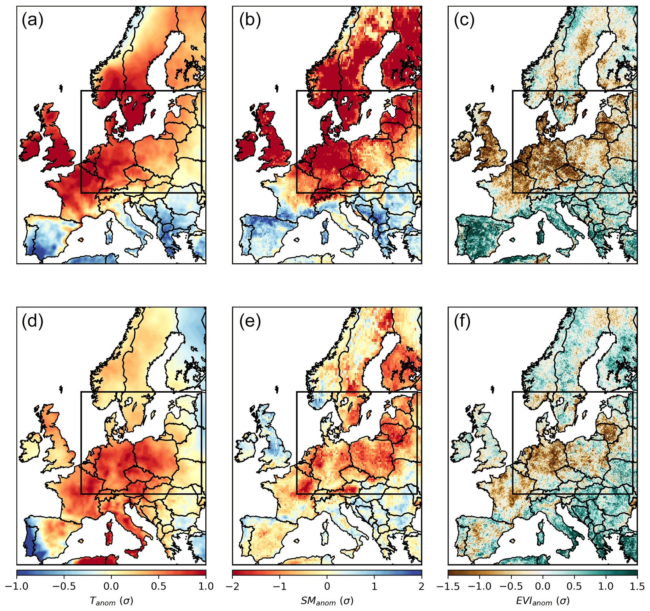
Figure 2Spatial patterns of temperature (Tanom), soil moisture (SManom), and EVI (EVIanom) anomalies during summer 2018 (a–c) and summer 2019 (d–f) for the study region. The study region corresponds to a domain with dry and hot conditions in both 2018 and 2019 summers (DH18 and DH19), delimited by the black rectangle.
For other modulating effects we evaluate how the spatial distribution of EVIanom residuals for DH18 and DH19 relates to climatic and ecological variables: SManom and Tanom in spring and summer, the number of dry months in the year of the DH event and the preceding year (i.e. 2017–2018 for DH18, and 2018–2019 for DH19), EVIanom in the preceding summer (), the number of dry months in a given year and its preceding year (DM), isohydricity (IsoH), and available water capacity (AWC, related to the maximum amount of water available for plants).
We include some of the drivers used to train the temporal climate-driven RF model to diagnose possible changes in the vulnerability explained by stronger vegetation sensitivity to climate anomalies than in the training period. is used to evaluate the preconditioning role of past extreme summers or disturbances (summer is the peak of the growing season in this region). The number of dry months and AWC are also included as they may explain non-linear relationships between SManom and vegetation stress. Isohydricity provides a measure of the degree of stomatal regulation by plants. Since many of these variables have strong spatial co-variation (e.g. Tanom and SManom, we evaluate their relationships with EVIanom residuals by calculating the partial rank correlation (Spearman's ρ) between each variable, controlling for the others separately. Since these effects might depend on land cover type, we analyse separately pixels with high and low tree cover.
To further evaluate how inter-annual legacy effects affect long-term vegetation dynamics, we apply a second temporal RF model to pixel-level EVIanom (Sect. 3.2.2) with as an additional predictor. The model is trained for the period 2002–2017 on 3×3 moving windows and is then used to predict EVIanom in DH18 and DH19. The resulting model residuals were then compared to those of the climate-driven RF model.
4.1 DH18 and DH19 impacts
Following the extreme summer in central Europe in 2018, mild temperatures and strong soil moisture deficits remained until January 2019, when SManom returned to normal conditions (Figs. B1 and B2). In central Europe, June 2019 was extremely hot, but July and August 2019 were milder (Fig. B1, Sousa et al., 2020), and soil moisture deficits became very pronounced in July (Fig. B2). In this region, except for during April 2019, the months preceding summer were not particularly dry and were even slightly wetter than average in February, March, and May, the latter also being colder than average. Therefore, the DH18 and DH19 constitute more a sequence of two compound events than a single drought. The areas experiencing severe dry and hot conditions in both summers correspond to a region covering central and eastern Europe and southern Sweden. This region is our study domain and indicated by the rectangle in Fig. 2). Both DH events led to vegetation browning, though negative EVIanom was more widespread in DH18 than DH19. Within the study region, 79 % of the area showing negative EVIanom in DH18 () also registered negative EVIanom in DH19 ().
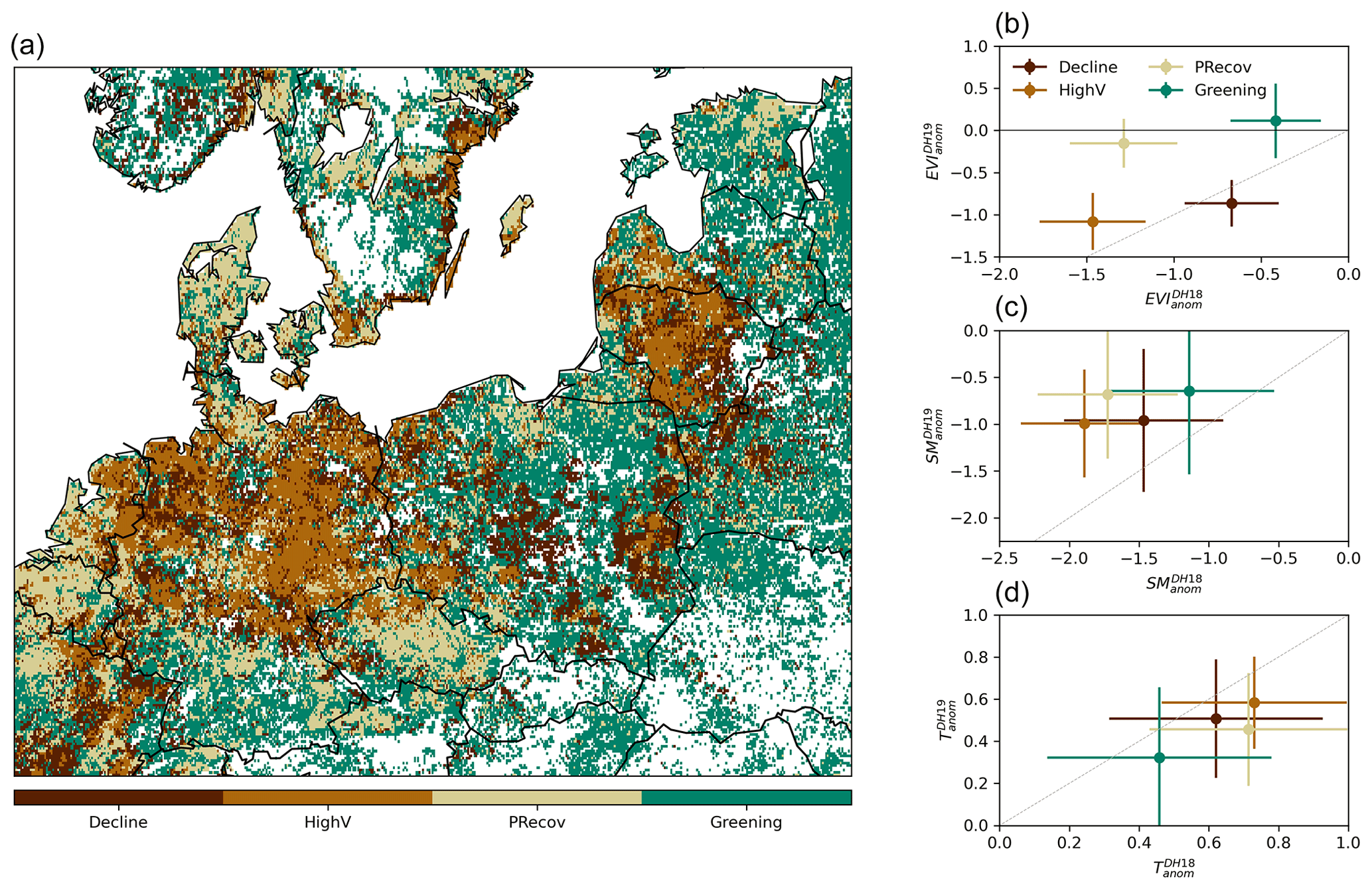
Figure 3Classification of impact groups within the study region in central Europe. Panel (a) shows the spatial distribution of the four clusters from unsupervised classification of (, ) values. The corresponding (, ) distribution in each cluster is indicated in panel (b) (circles indicate the spatial mean and lines the spatial standard deviation within each cluster). The corresponding distributions of SManom and Tanom pairs are shown in panels (c) and (d), respectively. The grey line indicates similar anomalies in the two DH events. Only pixels with negative are considered.
The spatial distribution of the clusters resulting from the unsupervised classification based on (, ) pairs and corresponding centroids are shown in Fig. 3a and b, as well as the corresponding (, ) and (, ) (Fig. 3c and d). The four clusters aggregate pixels according to different impacts in DH18 and DH19. One cluster, covering 20 % of the area, includes pixels with moderate impacts in DH18 and further browning in DH19, being therefore referred to as (CDecline) (dark brown, below the 1:1 line in Fig. 3a). This cluster is associated with mixed cover of forests (10 %–40 %, dominated by needle-leaved forest) and grasslands (15 %–60 %), (Fig. B3). Cluster CHighV (high vulnerability, covering 15 % of the area) corresponds to pixels experiencing strong impacts in both events and is associated with high grassland and cropland fractions and low tree cover. Pixels with strong impacts in DH18 and weakly negative , i.e. partial recovery in DH19 (CPRecov, 21 % of the area), are mainly dominated by croplands. Finally, a group of pixels shows moderate and positive (CGreening, 44 %), corresponding mostly to mixed forest–grassland pixels (30 %–65 % of forest, dominated by needle-leaved forest).
All clusters align along proportional DH18 : DH19 values of SManom and Tanom, with predominantly negative SManom and positive Tanom in both DH events but alleviation of soil moisture deficits and heat stress in DH19 compared to DH18 (Fig. 3). The two recovery clusters (CPRecov and CGreening) correspond to pixels with less severe drought conditions and milder temperatures in DH19, and CGreening corresponds to pixels where dry and hot conditions in DH18 were also more moderate. CHighV corresponds to pixels experiencing drier and hotter anomalies in both summers and accordingly shows stronger impacts. Cluster CDecline, however, shows increasing browning in DH19 in spite of drought and heat stress alleviation (Fig. 3). The distributions of climate anomalies for each cluster overlap each other and, in some cases, the 1:1 line, indicating that the intensity of the hazards (temperature, drought) cannot account for the resulting impacts alone.
4.2 Ecosystem vulnerability to DH18 and DH19
All clusters show significant positive linear relationships between summer EVIanom and SManom and negative linear relationships with Tanom in 2001–2017 (Fig. 4). The relationships include the two extreme summers of 2003 and 2015, which had comparable Tanom and SManom to DH18 and DH19 in most clusters. However, the long-term sensitivities estimated are robust even if these summers are excluded.
The results correspond to a general summer water-limited regime, especially in clusters CDecline, CHighV, and CPRecov, which show stronger sensitivities to Tanom and SManom (slopes in Fig. 4), and higher variance explained by both models (R2 0.58–0.68 for SManom and 0.49–0.55 for Tanom). For these clusters, EVIanom is below the 95 % confidence interval of the long-term linear relationships for DH18 (CPRecov and CHighV) and DH19 (CDecline and CHighV). SManom and Tanom in DH18 and DH19 are generally similar to those of 2003, but DH18 was drier than 2003 in CPRecov and CHighV.
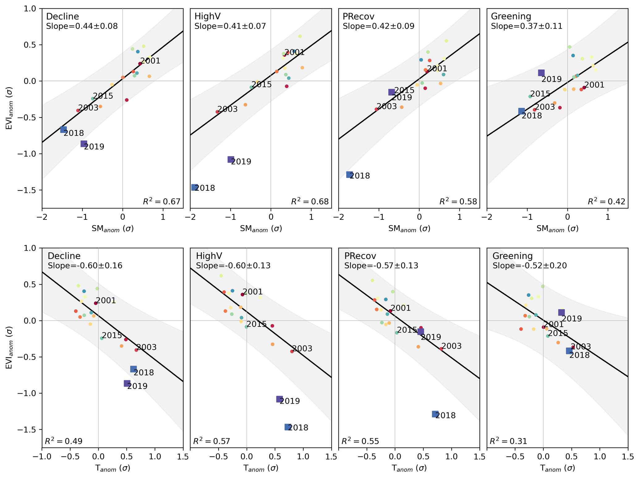
Figure 4Departure of EVIanom in DH18 and DH19 from long-term climate-driven variability. Relationship between EVIanom and SManom (top row) and between EVIanom and Tanom (bottom row) for each individual summer between 2001 and 2019 over the study region. The results are shown separately for the four clusters defined in Fig. 3. The black line and shaded areas show the relationship and respective 95 % confidence intervals obtained by ordinary least-squares linear regression between EVIanom and the respective climate variable for all years between 2001–2017. Values of (EVIanom, SManom) that deviate from the long-term relationships show increased sensitivity to climate anomalies, which can be a sign of increased vulnerability or decline. The colours indicate individual years, ranging from 2001 (red) to 2019 (purple), and square markers indicate 2018 and 2019.
These departures may be related with seasonal legacy effects from the warm spring in DH18 and/or the onset of non-linear responses to heat and drought. To account for these modulating effects, we model long-term (2001–2017) EVIanom–climate relationships using spring and summer SManom and Tanom as predictors using random forest regression (see Sect. 3.2.2). The model is able to predict 48 %–90 % (median and maximum out of bag score across pixels) of the pixel-level temporal variability of summer EVIanom in 2001–2017 (Fig. B4). Analysis of the variable importance shows that the model estimates summer water limitation and negative legacy effects from spring warming (Fig. B5), consistent with a summer water-limited regime and process-based modelling studies (Bastos et al., 2020a; Lian et al., 2020).
As in the linear case, the RF model estimates less negative or more positive EVIanom in DH18 and DH19 than observations (Fig. 5). The residuals are below the range of the training period for the high-impact clusters: CDecline and CPRecov in DH19 and DH18, respectively, and CHighV in both (Fig. 5c). In CGreening, residuals are predominantly positive (i.e. observed EVIanom more positive than predicted), but still partly overlap with the range of residuals in the training period (Fig. 5).
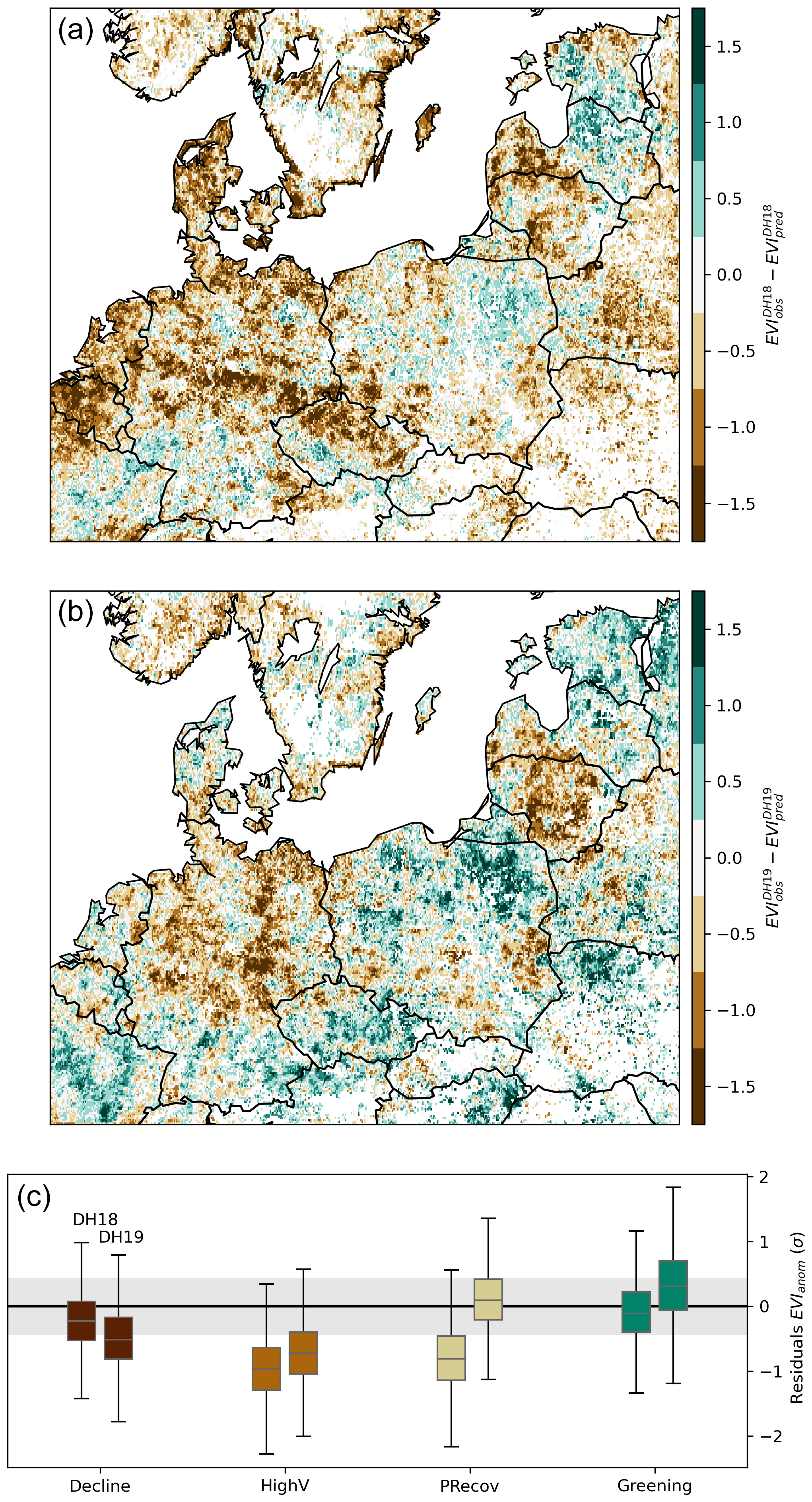
Figure 5Spatial distribution of EVIanom residuals in DH18 (a) and DH19 (b) estimated by the temporal RF model trained for 2001–2017 with spring and summer SManom and Tanom as predictors. The corresponding distribution per cluster for each DH event is shown by the boxplots in panel (c). The shaded grey envelope indicates the range of residuals in the training period.
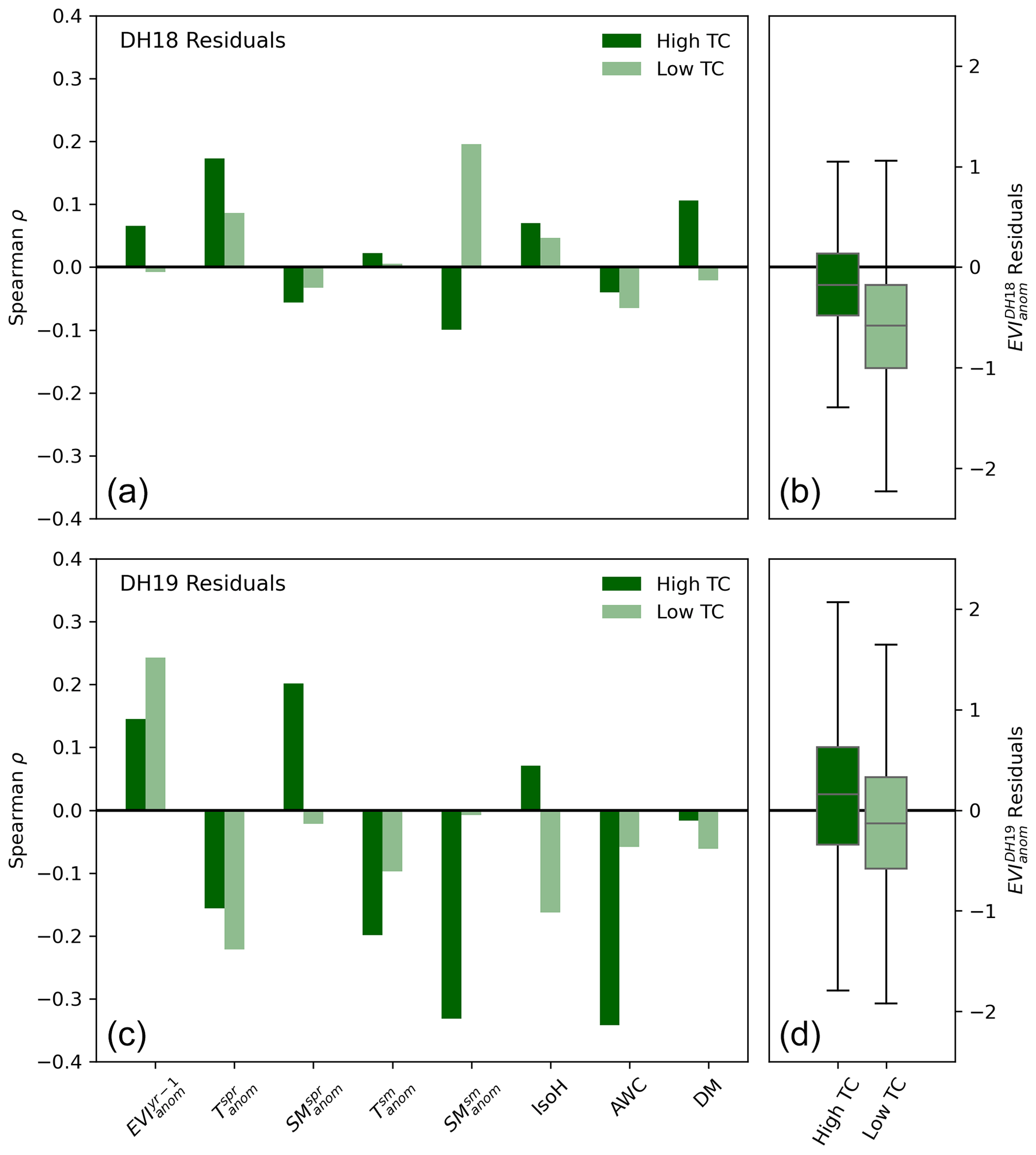
Figure 6Spatial partial correlation (Spearman) between EVIanom residuals and environmental variables in DH18 (a, b) and DH19 (c, d) for pixels with high (dark green, top 5 % tree cover fraction) and low (light green, lowest 5 % tree cover fraction) tree cover (a, c). High tree cover (TC) pixels have tree cover fractions above 58 % and low TC pixels have virtually no trees (TC<0.4 %). The variables considered are spring and summer Tanom and SManom (indicated by superscripts “spr” and “sm”, respectively), EVIanom in the previous growing season (EVIyr−1), plant isohydricity (IsoH), and the number of dry months (DM). Because of the large number of pixels considered, all correlations are significant (). Panels (b) and (d) show the distribution of residuals for pixels with high and low tree cover.
Pixels with high tree cover tend to show less negative or more positive residuals than pixels with low tree cover (<0.4 %) in both DH events (Fig. 6), but in DH19 the range of residuals in high tree cover pixels is larger than DH18, including pixels with strongly negative values. The partial rank correlation of the spatial distribution of EVIanom residuals with respect to different explanatory variables is shown for pixels with high and low tree cover in Fig. 6. Given the large number of pixels, all correlations are significant.
In DH18, Tanom in spring (, + for high and low tree cover) and summer SManom (, − for high tree cover and + for low tree cover) show the strongest relationships with EVIanom residuals. In DH19, (+), , and (−) show strong correlations, with consistent sign for both high and low tree cover pixels. DH19 residuals of pixels with high tree cover show strong correlation with SManom with opposite signs in spring (+) and summer (−) and with AWC (−). In DH19, pixels with low tree cover show negative correlation between IsoH and EVIanom residuals.
To test whether the importance of is particular to DH19 or if it reflects long-term inter-annual legacy effects of anomalies in vegetation activity, we fit a second temporal RF model where is used as an additional predictor (Figs. B4 and B6). Including vegetation condition in the previous summer improves the predictive power of the long-term RF model (72 %–97 % out-of-bag score, compared to 48 %–90 % for the model trained with climate drivers only). Even though the residuals for the training period are considerably reduced relative to the climate-driven model, the residuals for DH18 and DH19 are comparable.
4.3 DH18 and DH19 impacts simulated by LSMs
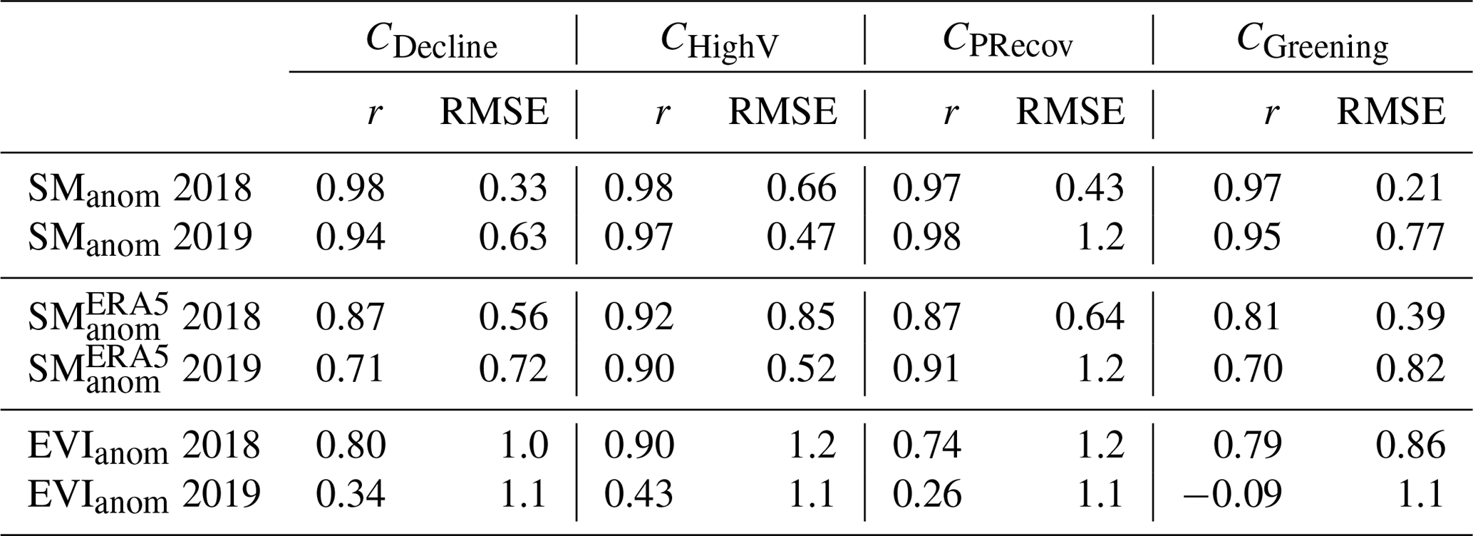
The GPP from the LSM multi-model ensemble mean matches the differences in impacts between clusters in DH18 well (Fig. 7a and b) and the temporal evolution of GPP anomalies during the 2018 growing season (April to September, Table 1), with correlations with EVIanom of 0.74–0.90. Even though the root-mean-squared error (RMSE) is comparable in the two growing seasons, the correlations of GPPanom with growing-season EVIanom are much lower in DH19 (−0.09 to 0.43). GPPanom by LSMs is above average in spring and early summer 2019 for all clusters, and anomalies in DH19 are either more positive or less negative compared to EVIanom.
LSMs simulate a stronger attenuation of drought compared to the observation-based SManom, albeit with consistent relative differences in SManom between clusters (compare Figs. B7 and 3). LSMs simulate the temporal evolution of SManom well in the two growing seasons, with high correlation with both SoMo.ml and (correlations of 0.81–0.98). The RMSE for simulated SManom is generally lower than that of GPPanom.
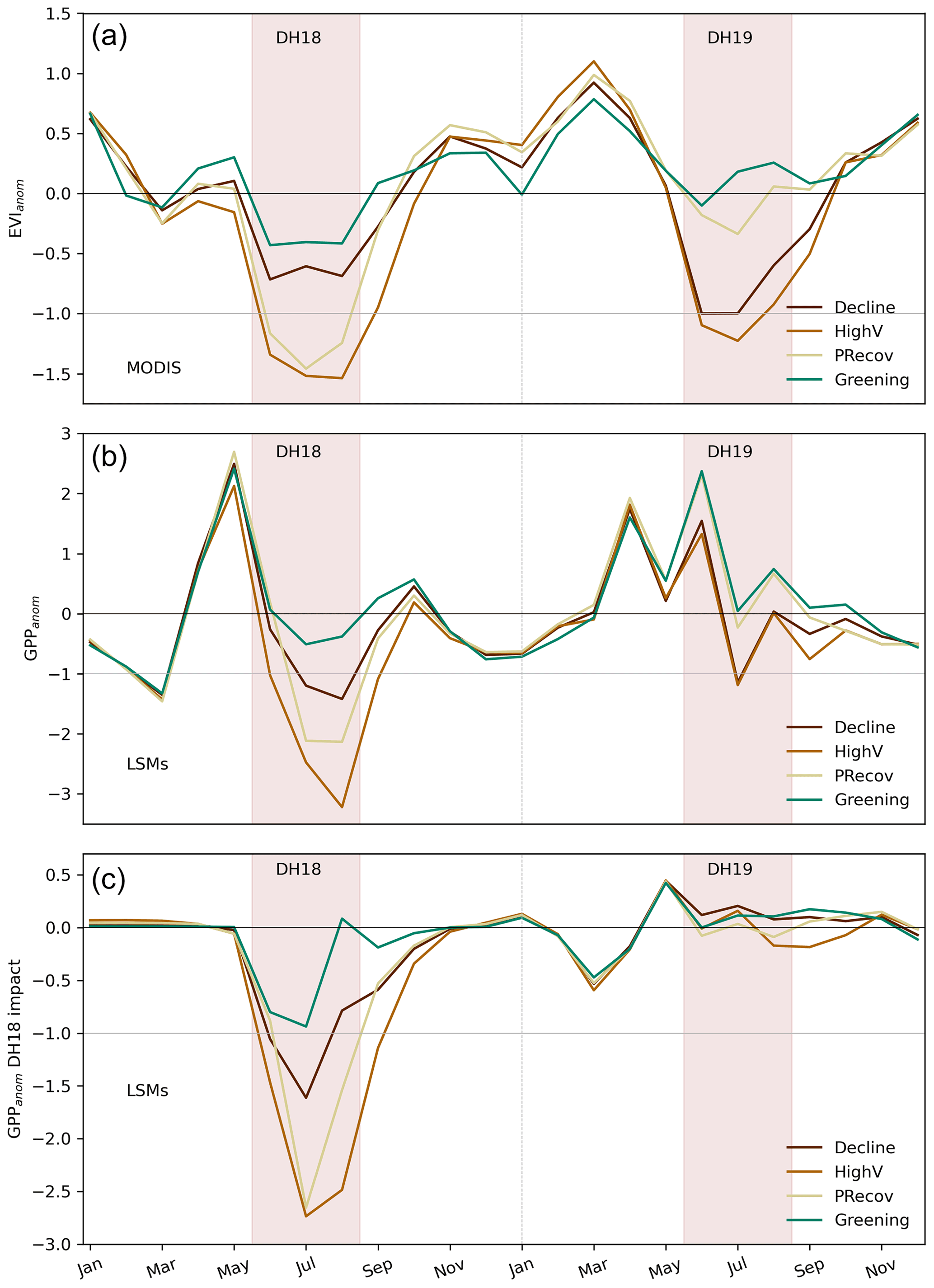
Figure 7Observed and process-based model simulations of 2018/19 impacts. Seasonal evolution of EVIanom (a) and standardised GPP anomalies (GPPanom, b) over the 2-year period for each cluster (defined in Fig. 3 and shown for LSM grid in Fig. B7). Panel (c) shows the difference between the reference and factorial simulations and indicates the impacts of DH18 on GPPanom simulated by models during the event and in the subsequent months until December 2019.
Table 1Correlation between growing season (gs, April–September) SManom simulated by LSMs with SManom from SoMo.ml and ERA5 and of EVIanom with GPP simulated by LSMs.
The sensitivity of GPPanom to simulated SManom and to Tanom (Fig. B8) is consistent with that of EVIanom in all clusters (Fig. 4), although for CPRecov and CGreening the LSMs estimate non-significant negative relationships between GPPanom and Tanom. The deviations of GPPanom from the linear response for CHighV and CPRecov in DH18 are correctly captured by LSMs but this is not the case for DH19 in CDecline.
5.1 Early signs of increased vulnerability
For three clusters covering 56 % of the pixels negatively impacted by DH18, the extremely low EVIanom in response to DH18 and DH19 could not be predicted from EVI–climate relationships in 2001–2017 (Figs. 4 and 5). These departures reveal increased sensitivity to dry and hot conditions and can be a sign of increased ecosystem vulnerability to such events. However, it should be noted that while we focused on pixels that were negatively impacted by DH18, some pixels in the regional domain selected showed greening, even in DH18 (Fig. 2). These regional asymmetries result in partial regional compensation of the DH18 impacts, as shown in Bastos et al. (2020b).
In both DH18 and DH19, higher tree cover fraction is associated with more positive or less negative residuals (Fig. 6), indicating that trees were more resistant to DH than grasses and crops. The predominance of crops and grasslands in CHighV, which had strong negative residuals in both events, and of high tree cover in CGreening also support this effect. Trees can better cope with drought with their deeper rooting depth (Fan et al., 2017) and through the use of carbon reserves to support activity under stress conditions (Wiley, 2020). Moreover, some trees and grasses with stronger stomatal regulation can buffer the drought progression and its impacts by avoiding hydraulic failure (McDowell et al., 2020; Teuling et al., 2010). This is reflected in the small but positive relationship between isohydricity and EVIanom residuals in pixels with high tree cover.
Increased vulnerability may be explained by modulating effects of global change on vegetation condition (e.g. “hotter droughts”, Allen et al., 2015, Fig. 1) and, in the case of DH19, it may be further linked to inter-annual legacies from the impact of DH18. The first should be expressed by relationships between EVIanom residuals and climatic variables. The latter are more difficult to assess without comprehensive data about different competing factors, e.g. defoliation or damage from embolism (Ruehr et al., 2019), higher susceptibility to diseases and pests due to reduced health (McDowell et al., 2020) or increased hazard of insect disturbances due to warm conditions (Rouault et al., 2006; Suzuki et al., 2014). The relationships between EVIanom residuals and provide an approximation but do not allow the identification of the underlying drivers.
In DH18, we find a positive effect of spring warming in vegetation growth, leading to weaker departures from long-term vegetation–climate relationships (observed EVIanom more positive or less negative than modelled), but with associated water depletion amplifying the impacts of DH18 in summer in pixels dominated by grasslands and crops (low tree cover in Fig. 6). These results are in line with Bastos et al. (2020a) that showed contrasting seasonal legacy effects of warm springs in cropland- versus forest-dominated regions.
On the contrary, spring and summer in 2019 (or cooling, see Fig. B1) are negative correlated with EVIanom residuals in both high and low tree cover pixels. This indicates increasing damage from heat stress, for example due to reductions in evapotranspirative cooling (Obermeier et al., 2018) or cascading impacts of compound heat and drought, such as insect attacks (Rouault et al., 2006).
Including in the long-term RF regression model improves the predictive skill for 2001–2017 but does not reduce the residuals in DH18 and DH19. The high correlation between EVIanom residuals and in DH19 can indicate either that pixels strongly impacted by DH18 were associated with amplified impacts by DH19 (negative residuals) or that pixels affected moderately by DH18 (less negative ) were associated with positive residuals, i.e. stronger recovery. Damage to roots and tissues or depletion of carbon reserves from DH18 leading to higher vulnerability to DH19 could explain the positive correlation in high tree cover pixels in CDecline. Conversely, the moderate DH18 impacts in CGreening may have resulted in increased resistance to DH19. The strong correlation found in low tree cover pixels is surprising though, as European crop species tend to be annual plants, and annual species can also be found in many grasslands. For these pixels, it is more likely that the positive correlation is explained by management practices, e.g. through earlier harvest or active reduction of stand density in DH19 (Bodner et al., 2015).
CDecline stands out from the other clusters, in that browning is found in spite of drought alleviation in DH19. The strong negative correlation of residuals with and AWC in forest-dominated pixels is counter-intuitive and suggests that other environmental effects not considered in our analysis may modulate DH19 impacts. Insect outbreaks are a potential candidate to explain such effects: the stronger correlation of residuals with in DH19 could reflect increased susceptibility of impaired trees, combined with favourable climatic conditions for insect growth, reflected in stronger negative effects of in DH19 in high tree cover pixels.
Results from field inventories and forest plots support this hypothesis. Increased tree mortality and insect outbreaks in central Europe during 2018 have been reported (Schuldt et al., 2020). A recent assessment by the German Federal Ministry for Food and Agriculture (BMEL, 2020) reported crown damage in 36 % of all tree types in summer 2019, a 7 % increase compared to 2018 and predominating in trees over 60 years of age. According to this report, the mortality rate in both needle-leaved and broad-leaved trees almost tripled from 2018 to 2019. Although no large-scale data on insect outbreaks are currently available, local authorities in regions where CDecline is prevalent report an increase in tree mortality from bark beetle infestations: the Environment Ministry of North Rhine-Westphalia in western Germany reported soaring rates of spruce affected by severe bark beetle infestations, from about 1 % in 2018 to over 12 % in 2019 (MULNV-NRW, 2019). In the Czech Republic, rates of spruce damaged by bark beetles more than tripled, leading to increased mortality (Hlásny et al., 2021). In Belgium, a “bark beetle task force” was created in September 2018 by the economic office of Wallonia (OEW, 2018). Increased tree mortality and bark beetle infestations have also been reported in eastern France (ONF, 2020).
5.2 Implications for Earth system modelling
Temperate ecosystems are an important global sink of CO2 (Pan et al., 2011) and are not usually considered hotspots of drought risk and environmental degradation under climate change (Vicente-Serrano et al., 2020). Our results show that the past two extreme summers in central Europe reveal the first signs of large-scale enhanced vulnerability in response to DH events (CHighV, CPRecov) and of potential degradation trajectories induced by consecutive events (CDecline). Even though it is limited to 20 % of the study area, the patterns in CDecline highlight the risks associated with more frequent and intense droughts and heatwaves expected in the coming decades (Barriopedro et al., 2011; Boergens et al., 2020; Hari et al., 2020). At the same time, progressive warming conditions can increase the likelihood of compound occurrence of multiple disturbances, such as droughts and insect outbreaks, which are both promoted by warm and dry conditions. Interactions between compounding disturbances can further contribute to forest C losses (Seidl et al., 2017; Kleinman et al., 2019). To anticipate such impacts, process-based modelling of ecosystem response to such events is needed.
The LSMs perform well in simulating the magnitude and evolution of productivity anomalies in 2018 but not in 2019. The recovery simulated by LSMs in DH19 can be partly explained by a strong recovery of modelled soil moisture (Fig. B7) but may also result from limited ability of LSMs to simulate changes in ecosystem vulnerability during the two DH events. The latter is supported by the fact that simulated SManom shows good agreement in the temporal evolution of soil moisture anomalies with both observation-based datasets but not of GPPanom (Table 1).
The comparison of the reference and factorial simulations allows showing that the poor performance in 2019 may be related with interannual legacy effects. LSMs estimate legacies from DH18 only in the early growing season (March to May 2019) but do not estimate any legacy effects in summer (Fig. 7 bottom panel). The poor relationships between EVIanom and simulated GPPanom in response to DH19 indicate that processes controlling legacy effects such as damage from embolism, carbon starvation, and resulting tree mortality or disturbances induced by drought and heat, such as insect outbreaks, currently missing in LSMs, likely explain the amplified impacts of DH19.
LSMs are known to have limited ability to simulate drought-induced stress and tree mortality (Wang et al., 2012) and lack impacts of biotic disturbances, although rudimentary approaches have been attempted (Kautz et al., 2018). These model shortcomings add to limitations in simulating soil moisture variability and transitions between energy-limited and water-limited regimes.
The summers of 2018 and 2019 were both exceptionally hot and dry over central Europe, and both were associated with widespread vegetation browning and tree mortality events. Here we propose an approach that analyses this event as a combination of three types of compound events (Zscheischler et al., 2020) that consider (i) the compound effects of hot and dry conditions, (ii) the effect of repeated stress conditions in 2019, and (iii) the legacy effects from DH18 impacts in preconditioning the impacts of DH19. Using statistical and process-based modelling, we quantify these effects and identify modulating effects, e.g. land cover composition. This approach can be extended to other types of events that may not fall in a single type of compound event.
Based on remote sensing data, we find signs of degradation trajectories in 20 % of the study area, with vegetation browning in spite of drought alleviation in DH19. We showed that inter-annual legacies from DH18 played an important preconditioning role in amplifying the impacts of DH19. While LSMs simulated the impacts of the first event (DH18) well, they showed limited skill in simulating the impacts of the subsequent compound event (DH19).
Our results show that compounding effects of multiple and repeated stressors and ecological dynamics can result in non-linear and unexpected impacts (Schuldt et al., 2020) that LSMs still cannot realistically simulate. Attribution of inter-annual legacy effects from DH18 and of LSM errors to internal processes (e.g. drought-induced damage and mortality) or others such as insect outbreaks remains challenging because up-to-date datasets on tree mortality and tree carbon reserves or spatially explicit information on biotic disturbances are very limited.
Since extreme DH events are projected to become more common in the coming decades, better understanding the interactions and feedbacks between climate extremes, natural disturbances, and ecosystem dynamics is fundamental to anticipate threats to the stability of forests in the temperate regions and elsewhere. Overlooking these effects may result in an overestimation of the resilience of the CO2 sink to climate change.
Land surface and global dynamic vegetation model simulations
We have used output of gross primary productivity (GPP) and simulated soil moisture from seven models that followed the protocol and extended the simulations in Bastos et al. (2020a) up to 2019. These models are ISBA-CTRIP (Joetzjer et al., 2015), JSBACH (Mauritsen et al., 2018), LPJ-GUESS (Smith et al., 2014), LPX-Bern (Lienert and Joos, 2018), OCN (Zaehle et al., 2010), ORCHIDEE (Krinner et al., 2005), and SDGVM (Walker et al., 2017).
The model simulations were run for most models at 0.25∘ spatial resolution for the European domain (32–75∘ N and −11–65∘ E), following a spin-up to equilibrate carbon pools. For the reference simulation, the models were forced with observed CO2 concentration from NOAA/ESRL and changing climate between 1979 and 2019 from ERA5 and fixed land cover map from 2010 from LUH2v2 (Hurtt et al., 2011). An additional simulation was run where the models were forced with changing climate, except June–August 2018, where climatological summer climate conditions were used to force the models as described in Bastos et al. (2020a). This simulation, extended up to December 2019, allows for evaluating the direct impact of DH18 and its inter-annual legacy effects.
For more details about the simulation protocol, we refer the reader to Bastos et al. (2020a).
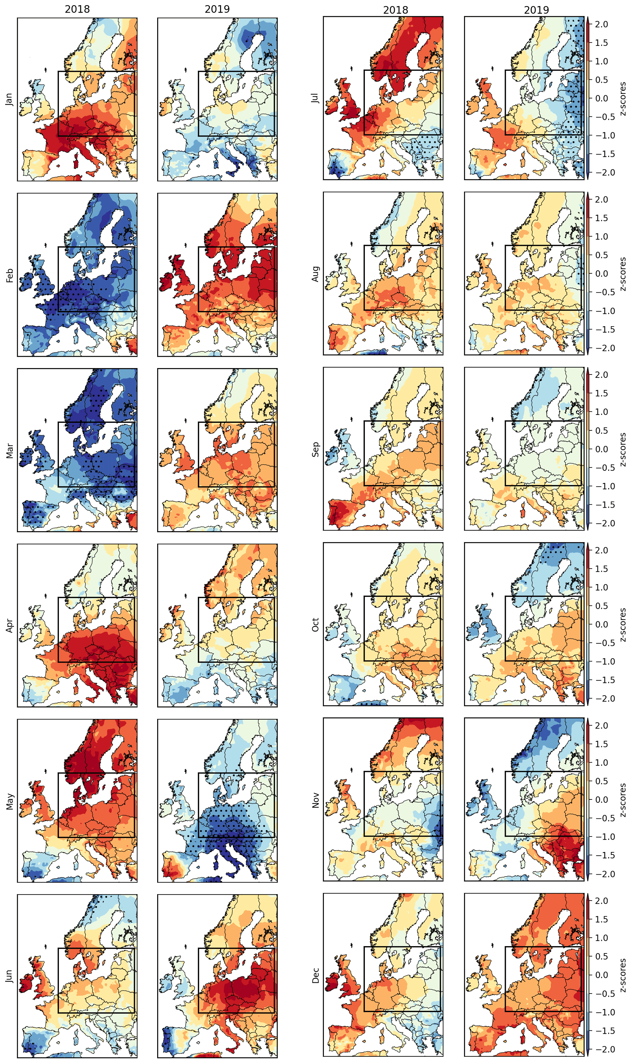
Figure B1Monthly temperature anomalies during 2018 and 2019. The rectangle indicates the study region.
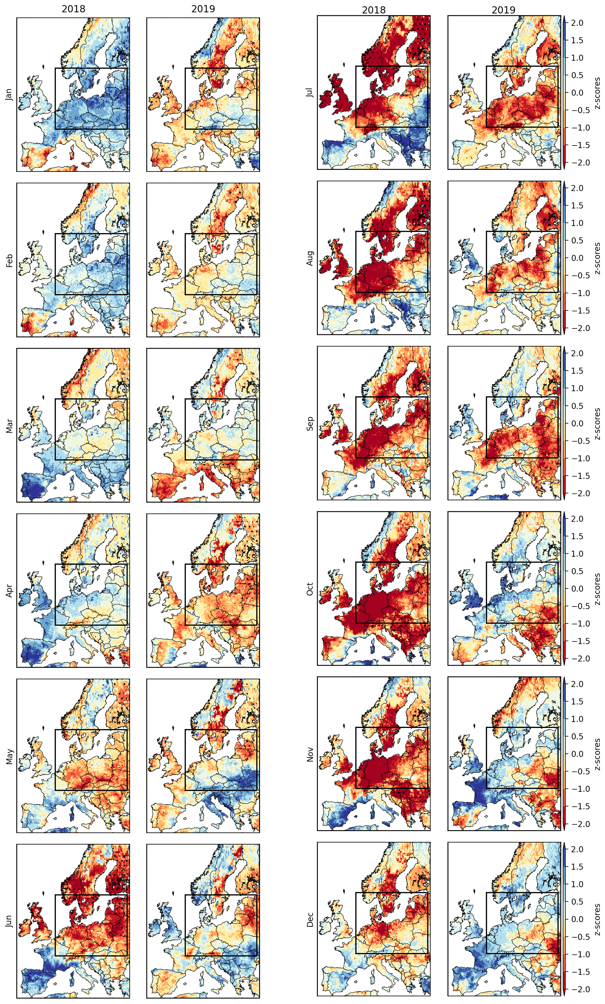
Figure B2Monthly soil moisture anomalies during 2018 and 2019. The rectangle indicates the study region, i.e. the areas experiencing drought conditions () during both DH18 and DH19.
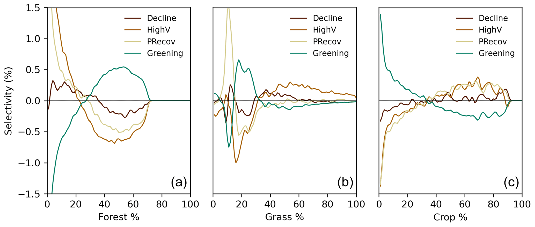
Figure B3Selectivity of different land cover composition for each cluster (Fig. 3). Selectivity is evaluated as the difference between the probability distribution of a given land cover type (forest, a; grassland, b; cropland, c) and the probability distribution of that land cover type in the selected region. If selectivity is positive, the cluster is preferentially composed by the given land cover type and the opposite for negative values. The 2018 land cover classification maps from ESA CCI-LC are used.
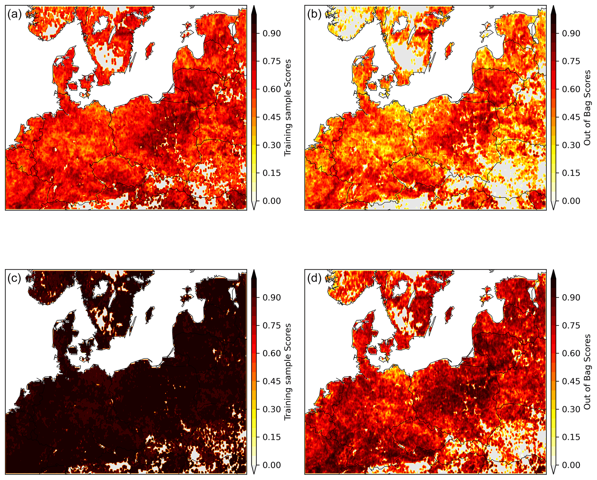
Figure B4Performance of the temporal RF model in predicting EVIanom given by the out-of-bag scores. Panels (a) and (b) show the scores for the climate-driven RF model, and panels (c) and (d) show the corresponding results for the same model but including as an additional predictor.
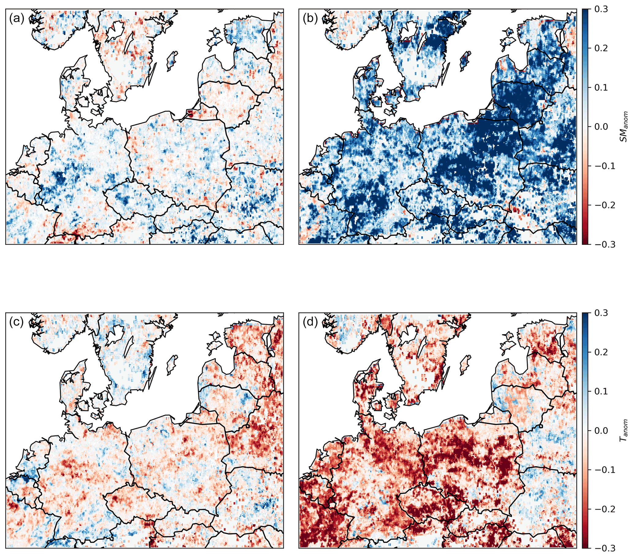
Figure B5Importance of the four predictors used in the RF model to predict EVIanom in spring (a, c) and summer (b, d), SManom (a, b), and Tanom (c, d) calculated from the Shapley additive explanation values.
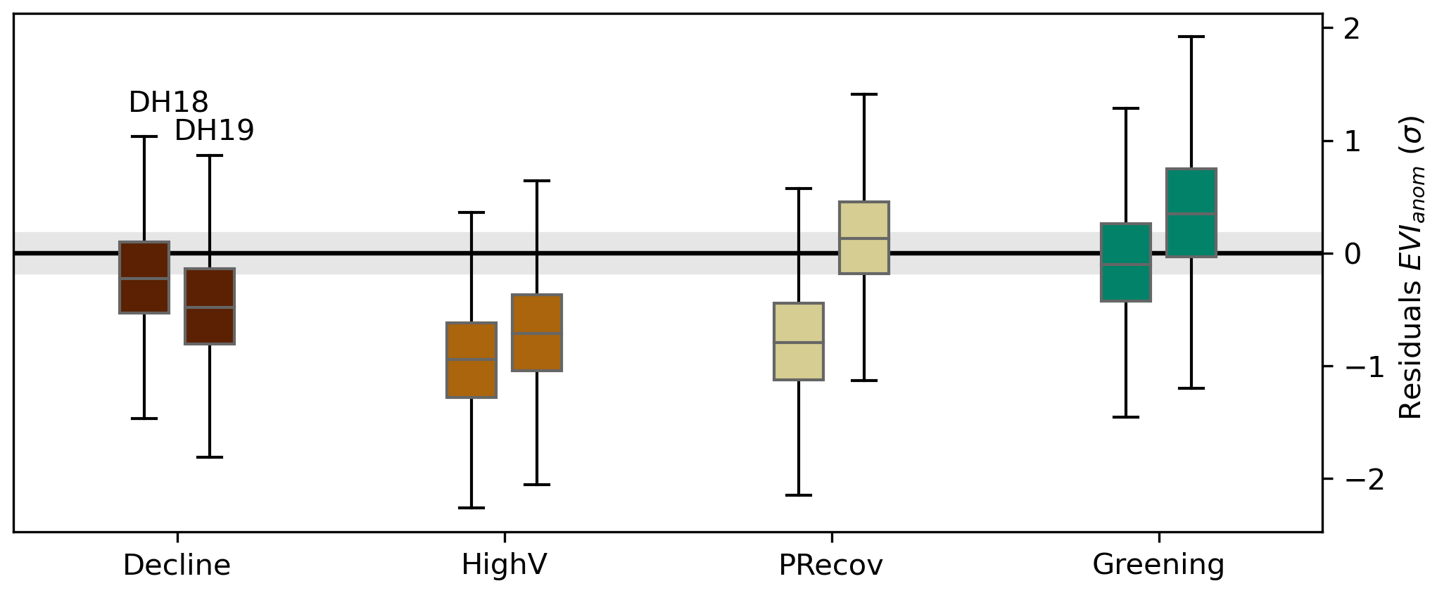
Figure B6The same as in Fig. 5c but for the RF model trained using spring and summer SManom and Tanom as predictors, as well as .
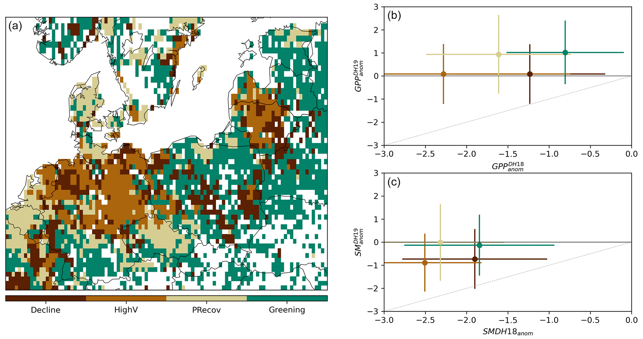
Figure B7Panel (a) shows the spatial distribution of the four clusters from unsupervised classification of (, ) values remapped to the coarser grid of LSMs. The corresponding (, ) values simulated by the multi-model mean in each cluster are indicated in (b) (circles indicate the spatial mean and the lines spatial standard deviation within each cluster). The corresponding distribution of simulated SManom pairs in each cluster are shown in (c). The grey line indicates similar anomalies in the two DH events.
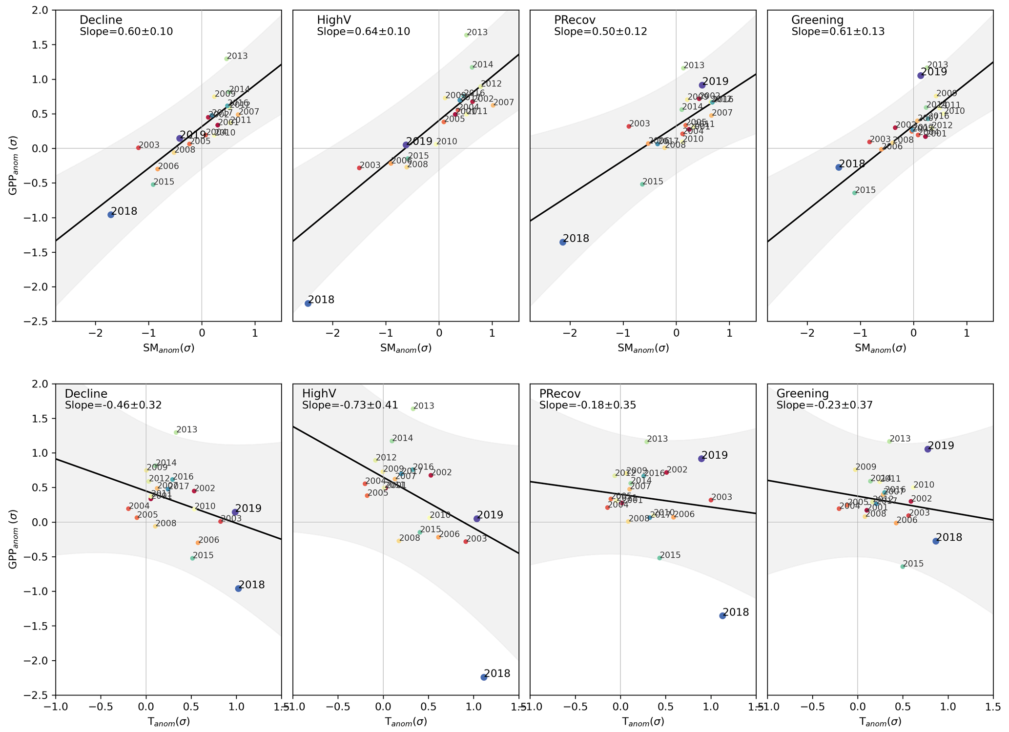
Figure B8The same as Fig. 4 but for GPP and soil moisture anomalies simulated by a subset of land surface models from (Bastos et al., 2020a) extended up to December 2019.
The MOD13C1 data are available through NASA's data catalogue at https://lpdaac.usgs.gov/products/mod13c1v006/ (last access: , NASA Earth Data, 2021). SoMo.ml v1.0 is publicly available via https://doi.org/10.17871/bgi_somo.ml_v1_2020 (O and Orth, 2021). Isohydricity fields are available at https://github.com/agkonings/isohydricity (last access: 25 August 2020; Konings et al., 2017). AWC data are provided by the European Soil Data Centre (ESDAC) through http://esdac.jrc.ec.europa.eu (last access: 20 August 2020). The multimodel mean fields from the LSMs are available at https://doi.org/10.6084/m9.figshare.16645123.v4 (Bastos et al., 2021). The individual LSM model outputs are available upon request to abastos@bgc-jena.mpg.de.
AB designed the study and methodology, conducted the data analysis, and wrote the manuscript. RO, MR, PC, NV, and SZ contributed to initial development of study and to the first manuscript draft. SS and JP helped in designing the LSM simulation protocol, and SS coordinated the LSM modelling effort. SO provided the SoMo.ml dataset. PG contributed with expert knowledge. NV, SZ, PA, AA, PCM, EJ, SL, and TL ran the LSM simulations. All authors participated in the writing of the final version of the manuscript.
The authors declare that they have no conflict of interest.
Publisher's note: Copernicus Publications remains neutral with regard to jurisdictional claims in published maps and institutional affiliations.
This article is part of the special issue “Understanding compound weather and climate events and related impacts (BG/ESD/HESS/NHESS inter-journal SI)”. It is not associated with a conference.
Ana Bastos thanks Ulrich Weber for the preprocessing of the MODIS data and Corinne Le Quéré for providing updated atmospheric CO2 fields for the model simulations. We thank the European Soil Data Centre (ESDAC), http://esdac.jrc.ec.europa.eu, European Commission, Joint Research Centre for making AWC data available and Alexandra Konings for providing the isohydricity dataset.
Ana Bastos received funding
by the European Space Agency Climate Change Initiative ESA-CCI RECCAP2 project (ESRIN/ 4000123002/18/I-NB). Sebastian Lienert and Sönke Zaehle have
received funding from the European Union's Horizon 2020 research and innovation programme (project 4C, Climate-Carbon Interactions in the Coming Century (grant no. 821003)). Sebastian Lienert has received funding from SNSF (grant no. 20020172476). René Orth and Sungmin O acknowledge support by the German Research Foundation (Emmy Noether grant no. 391059971). ORCHIDEE simulations was performed using HPC resources from GENCI-TGCC (grant no. 2020-A0070106328).
The article processing charges for this open-access publication were covered by the Max Planck Society.
This paper was edited by Gabriele Messori and reviewed by three anonymous referees.
Albergel, C., Dutra, E., Bonan, B., Zheng, Y., Munier, S., Balsamo, G., de Rosnay, P., Muñoz-Sabater, J., and Calvet, J.-C.: Monitoring and forecasting the impact of the 2018 summer heatwave on vegetation, Remote Sensing, 11, 520, https://doi.org/10.3390/rs11050520, 2019. a
Allen, C. D., Breshears, D. D., and McDowell, N. G.: On underestimation of global vulnerability to tree mortality and forest die-off from hotter drought in the Anthropocene, Ecosphere, 6, 1–55, 2015. a, b
Anderegg, W. R. L., Hicke, J. A., Fisher, R. A., Allen, C. D., Aukema, J., Bentz, B., Hood, S., Lichstein, J. W., Macalady, A. K., McDowell, N., Pan, Y., Raffa, K., Sala, A., Shaw, J. D., Stephenson, N. L., Tague, C., and Zeppel, M.: Tree mortality from drought, insects, and their interactions in a changing climate, New Phytol., 208, 674–683, 2015. a
Anderegg, W. R. L., Trugman, A. T., Badgley, G., Konings, A. G., and Shaw, J.: Divergent forest sensitivity to repeated extreme droughts, Nat. Clim. Change, 10, 1091–1095, https://doi.org/10.1038/s41558-020-00919-1, 2020. a
Ballabio, C., Panagos, P., and Monatanarella, L.: Mapping topsoil physical properties at European scale using the LUCAS database, Geoderma, 261, 110–123, 2016. a
Barriopedro, D., Fischer, E. M., Luterbacher, J., Trigo, R. M., and García-Herrera, R.: The Hot Summer of 2010: Redrawing the Temperature Record Map of Europe, Science, 332, 220–224, https://doi.org/10.1126/science.1201224, 2011. a, b
Bastos, A., Ciais, P., Friedlingstein, P., Sitch, S., Pongratz, J., Fan, L., Wigneron, J. P., Weber, U., Reichstein, M., Fu, Z., Anthoni, P., Arneth, A., Haverd, V., Jain, A. K., Joetzjer, E., Knauer, J., Lienert, S., Loughran, T., McGuire, P. C., Tian, H., Viovy, N., and Zaehle, S.: Direct and seasonal legacy effects of the 2018 heat wave and drought on European ecosystem productivity, Sci. Adv,, 6, eaba2724, https://doi.org/10.1126/sciadv.aba2724, 2020a. a, b, c, d, e, f, g, h, i, j, k, l, m
Bastos, A., Fu, Z., Ciais, P., Friedlingstein, P., Sitch, S., Pongratz, J., Weber, U., Reichstein, M., Anthoni, P., Arneth, A., Haverd, V., Jain, A., Joetzjer, E., Knauer, J., Lienert, S., Loughran, T., McGuire, P. C., Obermeier, W., Padrón, R. S., Shi, H., Tian, H., Viovy, N., and Zaehle, S.: Impacts of extreme summers on European ecosystems: a comparative analysis of 2003, 2010 and 2018, Philos. T. Roy. Soc. B, 375, 20190507, https://doi.org/10.1098/rstb.2019.0507, 2020b. a, b
Bastos, A., Orth, R., Reichstein, M., Ciais, P., Viovy, N., Zaehle, S., Peter, A., Arneth, A., Gentine, P., Joetzjer, E., Lienert, S., Loughran, T., McGuire, P., O, S., Pongratz, J., and Sitch, S.: Supplementary Data Bastos et al. ESD, figshare [data set], https://doi.org/10.6084/m9.figshare.16645123.v4, 2021. a
Beillouin, D., Schauberger, B., Bastos, A., Ciais, P., and Makowski, D.: Impact of extreme weather conditions on European crop production in 2018, Philos. T. Roy. Soc. B, 375, 20190510, https://doi.org/10.1098/rstb.2019.0510, 2020. a
BMEL: Ergebnisse der Waldzustandserhebung 2019, techreport, Bundesministerium für Ernährung und Landwirtschaft, Bonn, Germany, 2020 (in German). a
Bodner, G., Nakhforoosh, A., and Kaul, H.-P.: Management of crop water under drought: a review, Agron. Sustain. Dev., 35, 401–442, 2015. a
Boergens, E., Güntner, A., Dobslaw, H., and Dahle, C.: Quantifying the Central European Droughts in 2018 and 2019 with GRACE-Follow-On, Geophys. Res. Lett., 47, e2020GL087285, https://doi.org/10.1029/2020GL087285, 2020. a, b, c
Buermann, W., Forkel, M., O'Sullivan, M., Sitch, S., Friedlingstein, P., Haverd, V., Jain, A. K., Kato, E., Kautz, M., Lienert, S., Lombardozzi, D., Nabel, J. E. M. S., Tian, H., Wiltshire, A. J., Zhu, D., Smith, W. K., and Richardson, A. D.: Widespread seasonal compensation effects of spring warming on northern plant productivity, Nature, 562, 110–114, https://doi.org/10.1038/s41586-018-0555-7, 2018. a
Buras, A., Rammig, A., and Zang, C. S.: Quantifying impacts of the 2018 drought on European ecosystems in comparison to 2003, Biogeosciences, 17, 1655–1672, https://doi.org/10.5194/bg-17-1655-2020, 2020. a
Chan, W. C. H., Shepherd, T. G., Smith, K. A., Darch, G., and Arnell, N. W.: Storylines of UK drought based on the 2010–2012 event, Hydrol. Earth Syst. Sci. Discuss. [preprint], https://doi.org/10.5194/hess-2021-123, in review, 2021. a
Ciais, P., Reichstein, M., Viovy, N., Granier, A., Ogee, J., Allard, V., Aubinet, M., Buchmann, N., Bernhofer, C., Carrara, A., Chevallier, F., De Noblet, N., Friend, A. D., Friedlingstein, P., Grunwald, T., Heinesch, B., Keronen, P., Knohl, A., Krinner, G., Loustau, D., Manca, G., Matteucci, G., Miglietta, F., Ourcival, J. M., Papale, D., Pilegaard, K., Rambal, S., Seufert, G., Soussana, J. F., Sanz, M. J., Schulze, E. D., Vesala, T., and Valentini, R.: Europe-wide reduction in primary productivity caused by the heat and drought in 2003, Nature, 437, 529–533, 2005. a, b
Coumou, D. and Rahmstorf, S.: A decade of weather extremes, Nature Clim. Change, 2, 491–496, https://doi.org/10.1038/nclimate1452, 2012. a
Coumou, D., Lehmann, J., and Beckmann, J.: The weakening summer circulation in the Northern Hemisphere mid-latitudes, Science, 348, 324–327, 2015. a
Didan, K., Munoz, A. B., Solano, R., and Huete, A.: MODIS vegetation index user's guide (MOD13 series), University of Arizona: Vegetation Index and Phenology Lab, Tucson, AZ USA, 2015. a
Dorigo, W. A., Wagner, W., Hohensinn, R., Hahn, S., Paulik, C., Xaver, A., Gruber, A., Drusch, M., Mecklenburg, S., van Oevelen, P., Robock, A., and Jackson, T.: The International Soil Moisture Network: a data hosting facility for global in situ soil moisture measurements, Hydrol. Earth Syst. Sci., 15, 1675–1698, https://doi.org/10.5194/hess-15-1675-2011, 2011. a
Drouard, M., Kornhuber, K., and Woollings, T.: Disentangling Dynamic Contributions to Summer 2018 Anomalous Weather Over Europe, Geophys. Res. Lett., 46, 12537–12546, https://doi.org/10.1029/2019gl084601, 2019. a
Fan, Y., Miguez-Macho, G., Jobbágy, E. G., Jackson, R. B., and Otero-Casal, C.: Hydrologic regulation of plant rooting depth, P. Natl. Acad. Sci. USA, 114, 10572–10577, 2017. a
Gessler, A., Bottero, A., Marshall, J., and Arend, M.: The way back: recovery of trees from drought and its implication for acclimation, New Phytol., 228, 1704–1709, https://doi.org/10.1111/nph.16703, 2020. a
Hamerly, G. and Elkan, C.: Learning the K in K-Means, in: Proceedings of the 16th International Conference on Neural Information Processing Systems, NIPS'03, 281–288, MIT Press, Cambridge, MA, USA, 2003. a
Hari, V., Rakovec, O., Markonis, Y., Hanel, M., and Kumar, R.: Increased future occurrences of the exceptional 2018-2019 Central European drought under global warming, Sci. Rep.-UK, 10, 12207, https://doi.org/10.1038/s41598-020-68872-9, 2020. a
Hersbach, H., Bell, B., Berrisford, P., Hirahara, S., Horányi, A., Muñoz-Sabater, J., Nicolas, J., Peubey, C., Radu, R., Schepers, D., Simmons, A., Soci, C., Abdalla, S., Abellan, X., Balsamo, G., Bechtold, P., Biavati, G., Bidlot, J., Bonavita, M., De Chiara, G., Dahlgren, P., Dee, D., Diamantakis, M., Dragani, R., Flemming, J., Forbes, R., Fuentes, M., Geer, A., Haimberger, L., Healy, S., Hogan, R. J., Hólm, E., Janisková, M., Keeley, S., Laloyaux, P., Lopez, P., Lupu, C., Radnoti, G., de Rosnay, P., Rozum, I., Vamborg, F., Villaume, S., and Thépaut, J.-N.: The ERA5 global reanalysis, Q. J. Roy. Meteor. Soc., 146, 1999–2049, https://doi.org/10.1002/qj.3803, 2020. a, b
Hlásny, T., Zimová, S., Merganičová, K., Štěpánek, P., Modlinger, R., and Turčáni, M.: Devastating outbreak of bark beetles in the Czech Republic: Drivers, impacts, and management implications, Forest Ecol. Manage., 490, 119075, https://doi.org/10.1016/j.foreco.2021.119075, 2021. a
Hurtt, G., Chini, L. P., Frolking, S., Betts, R., Feddema, J., Fischer, G., Fisk, J., Hibbard, K., Houghton, R., Janetos, A., et al.: Harmonization of land-use scenarios for the period 1500–2100: 600 years of global gridded annual land-use transitions, wood harvest, and resulting secondary lands, Clim. Change, 109, 117–161, 2011. a
Joetzjer, E., Delire, C., Douville, H., Ciais, P., Decharme, B., Carrer, D., Verbeeck, H., De Weirdt, M., and Bonal, D.: Improving the ISBACC land surface model simulation of water and carbon fluxes and stocks over the Amazon forest, Geosci. Model Dev., 8, 1709–1727, https://doi.org/10.5194/gmd-8-1709-2015, 2015. a
Kannenberg, S. A., Schwalm, C. R., and Anderegg, W. R. L.: Ghosts of the past: how drought legacy effects shape forest functioning and carbon cycling, Ecol. Lett., 23, 891–901, https://doi.org/10.1111/ele.13485, 2020. a
Kautz, M., Anthoni, P., Meddens, A. J., Pugh, T. A., and Arneth, A.: Simulating the recent impacts of multiple biotic disturbances on forest carbon cycling across the United States, Global Change Biol., 24, 2079–2092, 2018. a
Kirches, G., Brockmann, C., Boettcher, M., Peters, M., Bontemps, S., Lamarche, C., Schlerf, M., Santoro, M., and Defourny, P.: Land Cover CCI-Product User Guide-Version 2, ESA Public Document CCI-LC-PUG, UCL-Geomatics, Belgium, 2014. a
Kleinman, J. S., Goode, J. D., Fries, A. C., and Hart, J. L.: Ecological consequences of compound disturbances in forest ecosystems: a systematic review, Ecosphere, 10, e02962, https://doi.org/10.1002/ecs2.2962, 2019. a
Konings, A., Williams, A., and Gentine, P.: Sensitivity of grassland productivity to aridity controlled by stomatal and xylem regulation, Nat. Geosci., 10, 284–288, 2017 (data available at: https://github.com/agkonings/isohydricity, last access: 25 August 2020). a, b
Krinner, G., Viovy, N., de Noblet-Ducoudré, N., Ogée, J., Polcher, J., Friedlingstein, P., Ciais, P., Sitch, S., and Prentice, I. C.: A dynamic global vegetation model for studies of the coupled atmosphere-biosphere system, Global Biogeochem. Cycles, 19, GB1015, https://doi.org/10.1029/2003GB002199, 2005. a
Lian, X., Piao, S., Laurent, Z., Li, X., Li, Y., Huntingford, C., Ciais, P., Cescatti, A., Janssens, I. A., Peñuelas, J., Buermann, W., Chen, A., Li, X., Myneni, R. B., Wang, X., Wang, Y., Yang, Y., Zeng, Z., Zhang, Y., and McVicar, T. R.: Summer soil drying exacerbated by earlier spring greening of northern vegetation, Sci. Adv., 6, eaax0255, https://doi.org/10.1126/sciadv.aax0255, 2020. a, b, c
Lienert, S. and Joos, F.: A Bayesian ensemble data assimilation to constrain model parameters and land-use carbon emissions, Biogeosciences, 15, 2909–2930, https://doi.org/10.5194/bg-15-2909-2018, 2018. a
Lundberg, S. M. and Lee, S.-I.: A unified approach to interpreting model predictions, in: Advances in neural information processing systems, Curran Associates, Inc, available at: https://papers.nips.cc/paper/2017/hash/8a20a8621978632d76c43dfd28b67767-Abstract.html (last acccess: 12 October 2021), 4765–4774, 2017. a
Mauritsen, T., Bader, J., Becker, T., Behrens, J., Bittner, M., Brokopf, R., Brovkin, V., Claussen, M., Crueger, T., Esch, M., Fast, I., Fiedler, S., Fläschner, D., Gayler, V., Giorgetta, M., Goll, D. S., Haak, H., Hagemann, S., Hedemann, C., Hohenegger, C., Ilyina, T., Jahns, T., Jimenéz-de-la-Cuesta, D., Jungclaus, J., Kleinen, T., Kloster, S., Kracher, D., Kinne, S., Kleberg, D., Lasslop, G., Kornblueh, L., Marotzke, J., Matei, D., Meraner, K., Mikolajewicz, U., Modali, K., Möbis, B., Müller, W. A., Nabel, J. E. M. S., Nam, C. C. W., Notz, D., Nyawira, S.-S., Paulsen, H., Peters, K., Pincus, R., Pohlmann, H., Pongratz, J., Popp, M., Raddatz, T. J., Rast, S., Redler, R., Reick, C. H., Rohrschneider, T., Schemann, V., Schmidt, H., Schnur, R., Schulzweida, U., Six, K. D., Stein, L., Stemmler, I., Stevens, B., von Storch, J.-S., Tian, F., Voigt, A., Vrese, P., Wieners, K.-H., Wilkenskjeld, S., Winkler, A., and Roeckner, E.: Developments in the MPI-M Earth System Model version 1.2 (MPI-ESM 1.2) and its response to increasing CO2, J. Adv. Model. Earth Sy., 11, 998–1038, https://doi.org/10.1029/2018MS001400, 2018. a
McDowell, N., Pockman, W. T., Allen, C. D., Breshears, D. D., Cobb, N., Kolb, T., Plaut, J., Sperry, J., West, A., Williams, D. G., and Yepez, E. A.: Mechanisms of plant survival and mortality during drought: why do some plants survive while others succumb to drought?, New Phytol., 178, 719–739, 2008. a
McDowell, N. G., Allen, C. D., Anderson-Teixeira, K., Aukema, B. H., Bond-Lamberty, B., Chini, L., Clark, J. S., Dietze, M., Grossiord, C., Hanbury-Brown, A., Hurtt, G. C., Jackson, R. B., Johnson, D. J., Kueppers, L., Lichstein, J. W., Ogle, K., Poulter, B., Pugh, T. A. M., Seidl, R., Turner, M. G., Uriarte, M., Walker, A. P., and Xu, C.: Pervasive shifts in forest dynamics in a changing world, Science, 368, 6494, https://doi.org/10.1126/science.aaz9463, 2020. a, b
Miralles, D. G., Teuling, A. J., van Heerwaarden, C. C., and Vila-Guerau de Arellano, J.: Mega-heatwave temperatures due to combined soil desiccation and atmospheric heat accumulation, Nat. Geosci., 7, 345–349, https://doi.org/10.1038/ngeo2141, 2014. a
MULNV-NRW: Waldzustandsbericht NRW 2019 (in German), techreport, Ministerium für Umwelt, Landwirtschaft, Natur- und Verbraucherschutz des Landes Nordrhein-Westfalen, 40190 Düsseldorf, Germany, 2019. a
NASA Earth Data: MOD13C1v006, available at: https://lpdaac.usgs.gov/products/mod13c1v006/ (last access: 13 May 2020), NASA [data set], 2021. a
O, S. and Orth, R.: SoMo.ml – Global soil moisture generated from in situ measurements using machine learning, Max Planck Institute for Biochemisty [data set], available at: https://www.bgc-jena.mpg.de/geodb/BGI/somo_ml_v1.php, last access: 12 October 2021. a
Obermeier, W. A., Lehnert, L. W., Ivanov, M. A., Luterbacher, J., and Bendix, J.: Reduced Summer Aboveground Productivity in Temperate C3 Grasslands Under Future Climate Regimes, Earth's Future, 6, 716–729, https://doi.org/10.1029/2018ef000833, 2018. a, b
OEW: Scolytes.be, available at: http://www.scolytes.be/ (last access: 20 August 2020), 2018. a
ONF, O. N. D. F.: Epicéas, sapins, hêtres… Ces arbres qui souffrent de la sécheresse, Tech. rep., Office National des Fôrets, available at: https://www.onf.fr/onf/+/4bd::ces-arbres-forestiers-qui-souffrent-de-la-secheresse.html (last access: 14 October 2021), 2020. a
Orth, R., Zscheischler, J., and Seneviratne, S. I.: Record dry summer in 2015 challenges precipitation projections in Central Europe, Sci. Rep.-UK, 6, 28334, 2016. a
Pan, Y., Birdsey, R. A., Fang, J., Houghton, R., Kauppi, P. E., Kurz, W. A., Phillips, O. L., Shvidenko, A., Lewis, S. L., Canadell, J. G., Ciais, P., Jackson, R. B., Pacala, S. W., McGuire, A. D., Piao, S., Rautiainen, A., Sitch, S., and Hayes, D.: A Large and Persistent Carbon Sink in the World's Forests, Science, 333, 988–993, https://doi.org/10.1126/science.1201609, 2011. a
Panagos, P., Van Liedekerke, M., Jones, A., and Montanarella, L.: European Soil Data Centre: Response to European policy support and public data requirements, Land use policy, 29, 329–338, 2012. a
Peters, W., van der Velde, I. R., van Schaik, E., Miller, J. B., Ciais, P., Duarte, H. F., van der Laan-Luijkx, I. T., van der Molen, M. K., Scholze, M., Schaefer, K., Vidale, P. L., Verhoef, A., Wårlind, D., Zhu, D., Tans, P. P., Vaughn, B., and White, J. W. C.: Increased water-use efficiency and reduced CO2 uptake by plants during droughts at a continental scale, Nat. Geosci., 11, 744–748, 2018. a
Rouault, G., Candau, J.-N., Lieutier, F., Nageleisen, L.-M., Martin, J.-C., and Warzée, N.: Effects of drought and heat on forest insect populations in relation to the 2003 drought in Western Europe, Ann. Forest Sci., 63, 613–624, 2006. a, b, c
Ruehr, N. K., Grote, R., Mayr, S., and Arneth, A.: Beyond the extreme: recovery of carbon and water relations in woody plants following heat and drought stress, Tree Physiol., 39, 1285–1299, 2019. a, b
Samaniego, L., Thober, S., Kumar, R., Wanders, N., Rakovec, O., Pan, M., Zink, M., Sheffield, J., Wood, E. F., and Marx, A.: Anthropogenic warming exacerbates European soil moisture droughts, Nat. Clim. Change, 8, 421–426, https://doi.org/10.1038/s41558-018-0138-5, 2018. a, b
Schuldt, B., Buras, A., Arend, M., Vitasse, Y., Beierkuhnlein, C., Damm, A., Gharun, M., Grams, T. E. E., Hauck, M., Hajek, P., Hartmann, H., Hiltbrunner, E., Hoch, G., Holloway-Phillips, M., Körner, C., Larysch, E., Lübbe, T., Nelson, D. B., Rammig, A., Rigling, A., Rose, L., Ruehr, N. K., Schumann, K., Weiser, F., Werner, C., Wohlgemuth, T., Zang, C. S., and Kahmen, A.: A first assessment of the impact of the extreme 2018 summer drought on Central European forests, Basic Appl. Ecol., 45, 86–103, 2020. a, b
Seidl, R., Thom, D., Kautz, M., Martin-Benito, D., Peltoniemi, M., Vacchiano, G., Wild, J., Ascoli, D., Petr, M., and Honkaniemi, J.: Forest disturbances under climate change, Nat. Clim. Change, 7, 395–402, 2017. a
Seneviratne, S. I., Nicholls, N., Easterling, D., Goodess, C., Kanae, S., Kossin, J., Luo, Y., Marengo, J., McInnes, K., and Rahimi, M.: Changes in climate extremes and their impacts on the natural physical environment, Managing the risks of extreme events and disasters to advance climate change adaptation, A Special Report of Working Groups I and II of the Intergovernmental Panel on Climate Change (IPCC), Cambridge University Press, Cambridge, UK, and New York, NY, USA, 109–230, 2012. a, b
Seneviratne, S. I., Donat, M. G., Mueller, B., and Alexander, L. V.: No pause in the increase of hot temperature extremes, Nat. Clim. Change, 4, 161–163, https://doi.org/10.1038/nclimate2145, 2014. a
Sherriff, R. L., Berg, E. E., and Miller, A. E.: Climate variability and spruce beetle (Dendroctonus rufipennis) outbreaks in south-central and southwest Alaska, Ecology, 92, 1459–1470, 2011. a
Smith, B., Wårlind, D., Arneth, A., Hickler, T., Leadley, P., Siltberg, J., and Zaehle, S.: Implications of incorporating N cycling and N limitations on primary production in an individual-based dynamic vegetation model, Biogeosciences, 11, 2027–2054, https://doi.org/10.5194/bg-11-2027-2014, 2014. a
Sousa, P. M., Barriopedro, D., García-Herrera, R., Ordóñez, C., Soares, P. M. M., and Trigo, R. M.: Distinct influences of large-scale circulation and regional feedbacks in two exceptional 2019 European heatwaves, Communications Earth & Environment, 1, 48, https://doi.org/10.1038/s43247-020-00048-9, 2020. a, b, c
Sungmin, O. and Orth, R.: Global soil moisture data derived through machine learning trained with in-situ measurements, Sci. Data, 8, 170, https://doi.org/10.1038/s41597-021-00964-1, 2021. a
Suzuki, N., Rivero, R. M., Shulaev, V., Blumwald, E., and Mittler, R.: Abiotic and biotic stress combinations, New Phytol., 203, 32–43, https://doi.org/10.1111/nph.12797, 2014. a
Teuling, A. J., Seneviratne, S. I., Stockli, R., Reichstein, M., Moors, E., Ciais, P., Luyssaert, S., van den Hurk, B., Ammann, C., Bernhofer, C., Dellwik, E., Gianelle, D., Gielen, B., Grunwald, T., Klumpp, K., Montagnani, L., Moureaux, C., Sottocornola, M., and Wohlfahrt, G.: Contrasting response of European forest and grassland energy exchange to heatwaves, Nat. Geosci., 3, 722–727, https://doi.org/10.1038/ngeo950, 2010. a
Vicente-Serrano, S. M., McVicar, T. R., Miralles, D. G., Yang, Y., and Tomas-Burguera, M.: Unraveling the influence of atmospheric evaporative demand on drought and its response to climate change, Wiley Interdisciplinary Reviews: Climate Change, 11, e632, https://doi.org/10.1002/wcc.632, 2020. a
Walker, A. P., Quaife, T., van Bodegom, P. M., De Kauwe, M. G., Keenan, T. F., Joiner, J., Lomas, M. R., MacBean, N., Xu, C., Yang, X., et al.: The impact of alternative trait-scaling hypotheses for the maximum photosynthetic carboxylation rate (Vcmax) on global gross primary production, New Phytol., 215, 1370–1386, 2017. a
Wang, W., Peng, C., Kneeshaw, D. D., Larocque, G. R., and Luo, Z.: Drought-induced tree mortality: ecological consequences, causes, and modeling, Environ. Rev., 20, 109–121, https://doi.org/10.1139/a2012-004, 2012. a
Wiley, E.: Do Carbon Reserves Increase Tree Survival during Stress and Following Disturbance?, Current Forestry Reports, 6, 1–12, 2020. a
Zaehle, S., Friend, A. D., Friedlingstein, P., Dentener, F., Peylin, P., and Schulz, M.: Carbon and nitrogen cycle dynamics in the O-CN land surface model: 2. Role of the nitrogen cycle in the historical terrestrial carbon balance, Global Biogeochem. Cycles, 24, GB1006, https://doi.org/10.1029/2009GB003522, 2010. a
Zeri, M., Costa, J. M., Urbano, D., Cuartas, L. A., Ivo, A., Marengo, J., dos and Santos Alvalá, R. C.: A soil moisture dataset over the Brazilian semiarid region, Mendeley Data [data set], V2, https://doi.org/10.17632/xrk5rfcpvg.2, 2020. a
Zscheischler, J. and Fischer, E. M.: The record-breaking compound hot and dry 2018 growing season in Germany, Weather Climate Extremes, 29, 100270, https://doi.org/10.1016/j.wace.2020.100270, 2020. a
Zscheischler, J., Martius, O., Westra, S., Bevacqua, E., Raymond, C., Horton, R. M., van den Hurk, B., AghaKouchak, A., Jézéquel, A., Mahecha, M. D., Maraun, D., Ramos, A. M., Ridder, N. N., Thiery, W., and Vignotto, E.: A typology of compound weather and climate events, Nat. Rev. Earth Environ., 1, 333–347, https://doi.org/10.1038/s43017-020-0060-z, 2020. a, b