the Creative Commons Attribution 4.0 License.
the Creative Commons Attribution 4.0 License.
 | 06 Nov 2020
Semi-equilibrated global sea-level change projections for the next 10 000 years
Jonas Van Breedam
Heiko Goelzer
Philippe Huybrechts
The emphasis for informing policy makers on future sea-level rise has been on projections by the end of the 21st century. However, due to the long lifetime of atmospheric CO2, the thermal inertia of the climate system and the slow equilibration of the ice sheets, global sea level will continue to rise on a multi-millennial timescale even when anthropogenic CO2 emissions cease completely during the coming decades to centuries. Here we present global sea-level change projections due to the melting of land ice combined with steric sea effects during the next 10 000 years calculated in a fully interactive way with the Earth system model of intermediate complexity LOVECLIMv1.3. The greenhouse forcing is based on the Extended Concentration Pathways defined until 2300 CE with no carbon dioxide emissions thereafter, equivalent to a cumulative CO2 release of between 460 and 5300 GtC. We performed one additional experiment for the highest-forcing scenario with the inclusion of a methane emission feedback where methane is slowly released due to a strong increase in surface and oceanic temperatures. After 10 000 years, the sea-level change rate drops below 0.05 m per century and a semi-equilibrated state is reached. The Greenland ice sheet is found to nearly disappear for all forcing scenarios. The Antarctic ice sheet contributes only about 1.6 m to sea level for the lowest forcing scenario with a limited retreat of the grounding line in West Antarctica. For the higher-forcing scenarios, the marine basins of the East Antarctic Ice Sheet also become ice free, resulting in a sea-level rise of up to 27 m. The global mean sea-level change after 10 000 years ranges from 9.2 to more than 37 m. For the highest-forcing scenario, the model uncertainty does not exclude the complete melting of the Antarctic ice sheet during the next 10 000 years.
- Article
(13386 KB) - Full-text XML
-
Supplement
(6456 KB) - BibTeX
- EndNote


Modern sea-level rise started at the end of the 1800s and has accelerated over the course of the 20th century (Church and White, 2011; Hay et al., 2015) with an unprecedented rate over the observational era during the first part of the 21st century (Watson et al., 2015). The rate of sea-level rise was 2.5 times faster during the last decade than during most of the 20th century (Oppenheimer et al., 2019). So far, the horizon for most global mean sea-level change projections has been the end of the 21st century (Jackson and Jevrejeva, 2016; Kopp et al., 2017; Goelzer et al., 2020b; Seroussi et al., 2020). Sea-level change projections beyond 2300 are scarce (Clark et al., 2016). However, due to the long lifetime of carbon dioxide in the atmosphere (Archer et al., 2009b) and the thermal inertia of the climate system (Solomon et al., 2009; Gillett et al., 2011; Goelzer et al., 2012), sea level is expected to continue to rise on a multi-centennial to multi-millennial timescale. Moreover, the large ice sheets themselves have a very long response time to any perturbations (Golledge, 2020) with the longest response time exceeding several millennia for changes in the surface mass balance and ice discharge in Antarctica (Alley and Whillans, 1984; Mengel et al., 2016).
Several feedbacks in the climate system reinforce an initial perturbation and on a multi-millennial timescale, a climate-warming–methane feedback might initiate. The increase in polar temperatures slowly releases methane from permafrost regions and accelerates climate change on a centennial timescale (Schuur et al., 2015). It is believed that a warming ocean could potentially also release a massive amount of methane from methane clathrates, somewhat similar to what is thought to have happened at the Palaeocene–Eocene Thermal Maximum (PETM; Zeebe and Zachos, 2013). This event took place at about 56 Ma and was characterized by a rapid global temperature rise of more than 5 ∘C in addition to a strong background warming, probably caused by the massive release of methane from clathrate hydrates (Dickens, 2011). These methane hydrates were released due to thermodynamic changes in the sediments where the hydrates are stored and this might happen again under long-term future climate warming (Dean et al., 2018).
On a multi-millennial timescale, changes in land ice volume (mass contribution) together with ocean density changes from thermal expansion (thermosteric contribution) and haline contraction (halosteric contribution) are the main components contributing to global sea-level change (Miller et al., 2005). The mass contribution comes from melting or growing of the Antarctic ice sheet, the Greenland ice sheet, and glaciers and ice caps. The steric contribution is the expansion of ocean water when it gets warmer and less saline or, conversely, the contraction when water is cooling and gets saltier (Feistel, 2010). The magnitude of thermal expansion depends on the climatic temperature forcing and on the rate of oceanic heat uptake. Because of the large mass and slow turnover time of the deep ocean, the oceanic heat content (and hence thermal expansion) will continue to rise in the ocean for multiple centuries, even when surface warming has halted. Haline contraction – or the expansion of ocean water due to freshening – is a smaller, though not negligible component of steric sea-level change.
Physically based models have been used to study the different components contributing to global sea level on a multi-millennial timescale. For example, long-term ice sheet evolution and resulting sea-level change projections have been made for the next few millennia for the Greenland ice sheet (Charbit et al., 2008; Robinson et al., 2012; Applegate et al., 2015), the Antarctic ice sheet (Huybrechts, 1993; Golledge et al., 2015; Pollard et al., 2015; Winkelmann et al., 2015; DeConto and Pollard, 2016), or both (Vizcaíno et al. 2008; Huybrechts et al., 2011). Among those studies, few had a full coupling between the ice sheet, the ocean, and the atmospheric component (Charbit et al., 2008; Vizcaíno et al., 2008; Huybrechts et al., 2011). One study used a full coupling only between the ice sheets and the atmosphere (Robinson et al., 2012), while most other studies (Huybrechts, 1993; Applegate et al., 2015; Golledge et al., 2015; Pollard et al., 2015; Winkelmann et al., 2015; DeConto and Pollard, 2016) used ice sheet models that were one-way forced without the inclusion of freshwater forcing of the ocean or the albedo–temperature feedback.
Existing long-term sea-level change projections including both the changes in land ice volume and the steric components extend for the next 2000 years (Levermann et al., 2013) or 10 000 years (Clark et al., 2016). However, these studies did not take the full coupling between the ice sheets, the ocean, and the atmosphere into account, which becomes important when the ice sheets lose large volumes of freshwater. Goelzer et al. (2012) studied the committed sea-level rise at the end of 3000 CE with a coupled model approach for a range of idealized CO2 scenarios. So far, the study of semi-equilibrated sea-level changes including all components of future sea-level change with the incorporation of feedbacks between the climate components has not been performed because of the high computational cost. The trade-off between model complexity and model interactions on a multi-millennial timescale adopted here consists of the use of the Earth system model of intermediate complexity LOVECLIM with a lower resolution but with full coupling.
In this study, we project the global mean sea-level changes for the next 10 000 years in a fully interactive way between all major components in the climate system. The duration of the simulations allows the climate system to reach a semi-equilibrated state, a long time after the cessation of anthropogenic greenhouse gas emissions. The greenhouse gas forcing follows the Extended Concentration Pathway (ECP) scenarios (Meinshausen et al., 2011) to span the likely range in emission uncertainties with the inclusion of a methane emission feedback in a warming climate.
High-resolution general circulation models (GCMs) are the best tools to project climate changes until the end of the century or a few hundred years after that, but they are computationally too expensive to make millennial to multi-millennial projections. Earth system models of intermediate complexity (EMICs) have a lower resolution and therefore allow for longer simulations such as simulating the climate over the last millennium (Eby et al., 2013) or exploring climate–carbon-cycle feedbacks during the next 1000 years (Zickfeld et al., 2013). With recent progress in computational power, it is expected that Earth system models with a higher spatial resolution will be able to simulate the climate over the last millennium (Jungclaus et al., 2017). Here we make use of the EMIC LOVECLIMv1.3 (Goosse et al., 2010) for the projections of global sea-level change on a multi-millennial timescale. LOVECLIM is one of the few EMICs (together with CLIMBER and UVic; Eby et al., 2013) with an ice sheet component (AGISM) that is fully coupled to the other components of the climate system (ECBilt for the atmosphere; CLIO for the ocean and sea ice; VECODE for the terrestrial biosphere), allowing for multi-millennial projections of sea-level change. ECBilt is a quasi-geostrophic atmospheric model with truncation T21, corresponding to a resolution in longitude and latitude of approximately 5.625∘ and three vertical levels (Opsteegh et al., 1998). The surface air temperature in the coarse-resolution atmospheric component is extrapolated from higher levels based on reference profiles from NCEP-NCAR reanalysis (Kalnay et al., 1996). The surface wind in LOVECLIM is calculated as a fraction (0.8) of the surface wind speed at the 800 hPa level (Goosse et al., 2010). CLIO is a global free surface ocean GCM coupled to a thermodynamic sea-ice model, with a resolution of 3∘ in longitude and latitude and 20 unevenly spaced vertical levels (Goosse and Fichefet, 1999). AGISM, the ice sheet model component consists of 3-D thermomechanically coupled ice sheet models for the Greenland ice sheet and the Antarctic ice sheet (Huybrechts and de Wolde, 1999). The ice sheet models include an isostasy model that consists of an elastic lithosphere on top of a viscous asthenosphere to simulate bedrock elevation changes in response to ice sheet changes. They are run at a resolution of 10 km for the Greenland ice sheet and 20 km for the Antarctic ice sheet. The relatively coarse resolution is necessary to allow for long integrations. The global glacier melt algorithm is based on the model of Raper and Braithwaite (2006) that considers a total sea-level equivalent (SLE) of 0.241 m (mountain glaciers contain 41 % of this estimate, while the ice caps are responsible for the other 59 % of sea-level rise, SLR, potential). This is at the lower end of the range of total recent estimates of ice volume (0.24–0.40 m SLE) stored in all ∼ 215 000 glaciers on Earth (Farinotti et al., 2019), partly explained by the fact that the glacier model excludes glaciers in the periphery of the Greenland and Antarctic ice sheets. The steric sea-level change component is calculated based on regional changes in ocean temperature and salinity. The ocean carbon cycle is not activated and greenhouse gas concentrations are prescribed (see Sect. 3 and Appendix A).
The model has been used previously for ice sheet and climate change projections for periods in the past (Loutre et al., 2014; Goelzer et al. 2016a, b) and the future (Huybrechts et al., 2011; Goelzer et al., 2012). The version used here differs from LOVECLIMv1.3 for the Antarctic ice sheet component by including surface ablation on the ice shelves, an important process under future atmospheric warming. A tundra warming feedback is also included for retreating ice sheets by making a distinction between snow/ice albedo and tundra albedo. The snow/ice albedo is replaced by tundra albedo (with a lower albedo) once the ice sheet margin is retreating on land. In order to better represent the climate forcing for the ice sheet models, temperature and precipitation anomalies are applied to the average over a reference period (1970–2000) to eliminate the climatic model bias for the present day. The surface mass balance is calculated using the positive degree day (PDD) method for both ice sheets. The melt is parameterized based on the yearly sum of daily average temperatures above 0 ∘C to determine the melt potential. The melt potential is used to melt snow or ice, with different conversion factors (degree day factors) for snow and ice. The rain limit determines whether precipitation falls as snow or as rain. An increase in precipitation will add mass to the ice sheet surface as long as temperatures are lower than the rain limit (1 ∘C in our simulations). Retention and refreezing of meltwater in the snowpack are also included. The PDD model has the advantage that it is calculated on the high-resolution grid of the ice sheet model in comparison to an energy balance model from a coarse-resolution climate model. The Antarctic ice sheet model uses the shallow ice approximation (SIA) for grounded ice and the shallow shelf approximation (SSA) for the ice shelves coupled across a one-grid-cell-wide transition zone. Basal melting is calculated as a function of the mean oceanic heat input into the ice shelf cavities. Sea-level changes resulting from the melting of the marine-based parts of the Antarctic ice sheet are corrected for bedrock elevation changes (Goelzer et al., 2020a). The Greenland ice sheet model is identical to previous versions of the model employed within the LOVECLIM framework (Goelzer et al., 2012, 2016a, b). Both ice sheet models have recently participated in the ISMIP6 initiative (Goelzer et al., 2020b; Seroussi et al., 2020).
Since many physical parameters in a climate model are uncertain, LOVECLIM is used to explore the climate response for a large combination of climate model parameter sets (Loutre et al., 2011). Here we have evaluated four different model parameter sets by testing the sea-level contribution for the period 1900–2300 CE. The four model parameter sets (P11, P22, P32a, P32b; see Table S3 in the Supplement) differ in their sensitivity to the applied greenhouse forcing (P32b and P32a > P22 > P11) and freshwater forcing in the North Atlantic (P32a, P32b, and P22 > P11). All climate model parameter sets yield climate simulations in agreement with observations over the past 500 years (Loutre et al., 2011). Model parameter set P22 is chosen for the multi-millennial integrations because of its mid-range contribution to sea level at 2100 CE and 2300 CE in comparison with recent studies (Pörtner et al., 2019; Calov et al., 2018; Bulthuis et al., 2019; Tables S1–S2 and Fig. S1 in the Supplement) and its agreement in polar temperature forcing at the end of the 21st century. The mean annual temperature anomalies over the ice sheets for 2070–2100 relative to 1970–2005 (+4.6 ∘C over Greenland and +3.8 ∘C over Antarctica for Representative Concentration Pathway 8.5, RCP8.5) correspond well with the mid- to upper ranges of Atmosphere–Ocean General Circulation Model (AOGCM) projections over the polar regions (Fettweis et al., 2013; Barthel et al., 2020). With an equilibrium climate sensitivity of 2.3 ∘C, the model parameter set is at the lower end of IPCC AR5 estimates (likely range of 1.5–4.5 ∘C) due to a cold bias in the tropics.
The Greenland ice sheet and Antarctic ice sheet are spun-up from stand-alone experiments forced with reconstructed temperature forcing above the ice sheet following ice core records for respectively two and four glacial–interglacial cycles to carry their long-term ice sheet history (Huybrechts et al., 2011; Goelzer et al., 2012). A quasi-equilibrium experiment is run with the aim of getting a climate in equilibrium at 1500 CE with the ice sheet forcing. The ice sheet models in this experiment evolve very slowly for a fixed climate forcing. The climate model on the other hand is subject to changes in the ice sheet models (changes in freshwater flux, albedo, and height changes) and equilibrates to these boundary conditions. At the end of the quasi-equilibrium run (after 2500 years when the temperature and ice sheet volume changes become negligible), a steady state is reached. A control experiment with constant pre-industrial greenhouse gas forcing showed that the drift in climate and ice sheet components is negligible. The climate information present at the end of the quasi-equilibrium experiment is used as input for the initialization of the fully coupled experiments starting at 1500 CE.
The fully coupled model is run from 1500 to 2000 CE. LOVECLIM is forced during this historical period with known greenhouse gas concentrations, total solar irradiance, and volcanic forcing. Now, all components of LOVECLIM interact dynamically and are run as an ensemble of five members. The ensemble members are identical except for small perturbations in the initial boundary conditions of the atmospheric component. Next, the ensemble runs are iterated with an updated reference state for the ice sheet models to determine whether there is convergence for the climatic information (e.g. Greenland and Antarctic temperature forcing, oceanic heat content, and meridional overturning circulation variability). The experiment performing best at representing the climate over the last 500 years is chosen as input for the long-term future projections. The Greenland and Antarctic ice sheet geometry at the start of the future projections (2000 CE) is shown in Fig. 1.
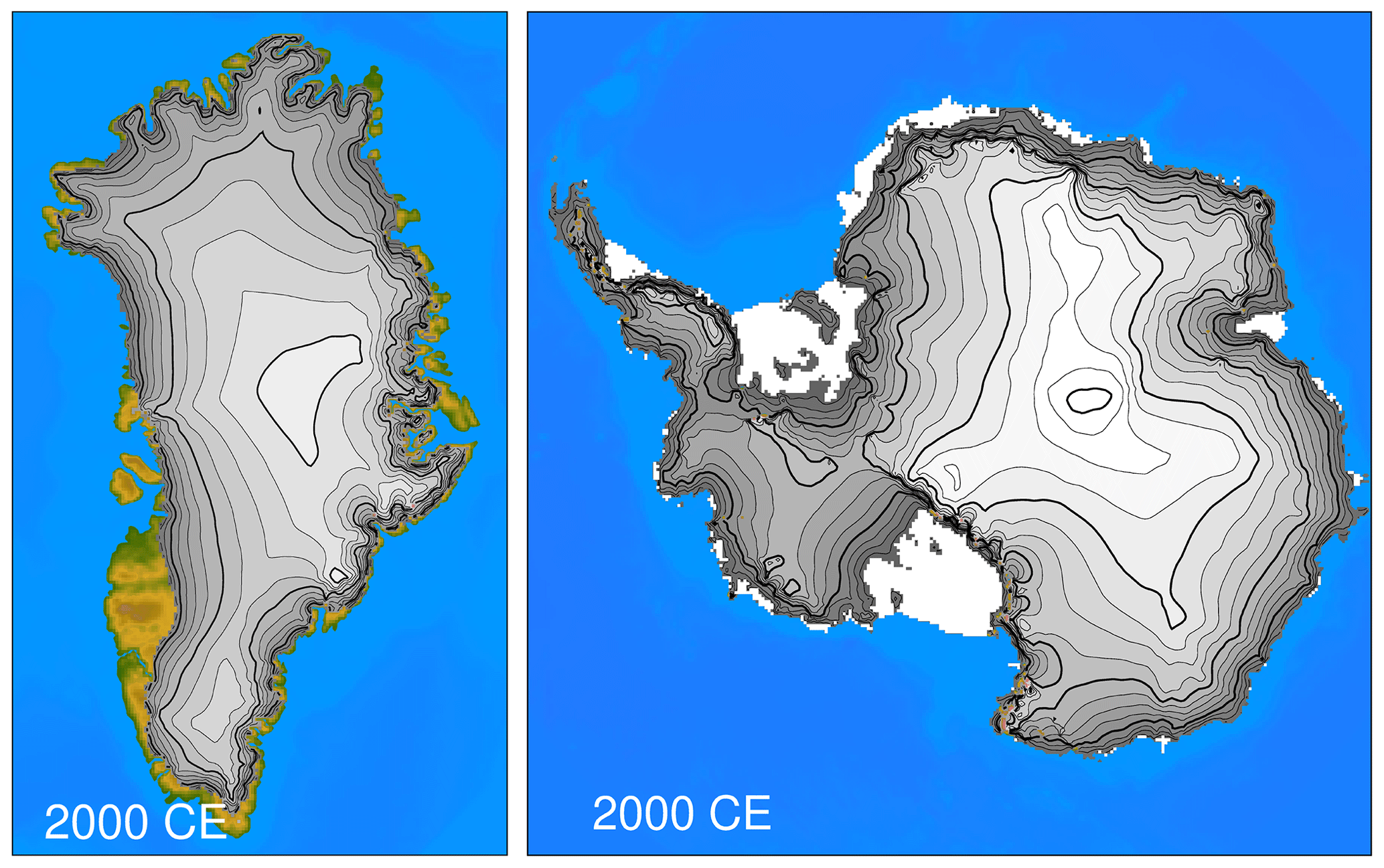
Figure 1The Greenland ice sheet and the Antarctic ice sheet geometry after the spin-up procedure at 2000 CE.
Six different forcing scenarios are constructed to span a large range of future greenhouse gas forcing. The main difference between the different scenarios is the atmospheric carbon dioxide forcing. Four of the CO2 forcing scenarios are extensions of the ECP scenarios (Meinshausen et al., 2011) and will be introduced here as Multi-Millennial Concentration Pathways (MMCPs) with the same designation as the RCP scenarios (MMCP2.6, MMCP4.5, MMCP6.0, and MMCP8.5). The scenarios range from a peak in the CO2 concentration of 443 ppmv in 2053 CE with temporarily negative emissions thereafter (MMCP2.6) to a peak of 1962 ppmv in 2250 CE (MMCP8.5). Estimates of the total recoverable carbon (oil, gas, lignite, and coal) reserves (the total exploitable carbon) and resources (total carbon mass stored on earth, including the non-exploitable carbon) are disputed, ranging from <1500 GtC reserves and 4000 GtC resources (Hasselmann et al., 2003) up to 2900 GtC reserves and 11 000 GtC resources (McGlade and Ekins, 2015). In this study, the MMCP scenarios (extended ECP scenarios with zero emissions after 2300 CE) are equivalent to a total cumulative emission ranging from less than 200 GtC for scenario MMCP2.6 to more than 5000 GtC for scenario MMCP8.5 relative to the year 2000 CE (see Appendix A: Table A3). This is comparable to the study from Clark et al. (2016) with an emission pulse of 1280–5120 GtC but well below the study from Winkelmann et al. (2015), which assumes a total carbon release of up to 10 000 GtC.
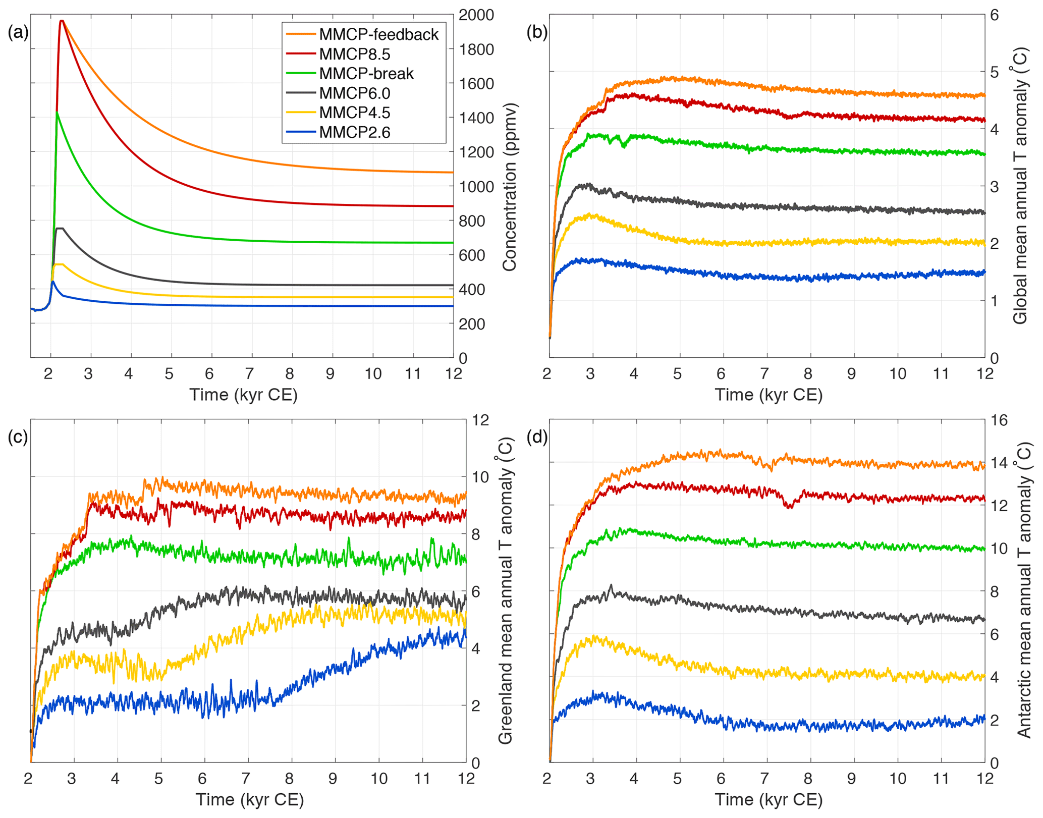
Figure 2(a) Atmospheric CO2 concentration scenario from 1500 CE to 12 000 CE for the six different forcing scenarios. (b) Global mean temperature change for the historical period 1500–2000 CE and the future projections, (c) Greenland mean temperature change, and (d) Antarctic mean temperature change for the six forcing scenarios. All temperature projections are shown as an anomaly to a reference period 1970–2000.
Two additional scenarios are constructed because of the large difference in emissions between MMCP6.0 and MMCP8.5 and to allow for an upper-end scenario that exceeds MMCP8.5 because of a methane emission feedback. The first one assumes that CO2 concentrations follow ECP8.5 but emissions will cease completely by the year 2150 CE. This scenario is referred to as MMCP-break and is an intermediate forcing scenario between MMCP6.0 and MMCP 8.5. The second additional scenario (MMCP-feedback) is similar to MMCP8.5 up to 2250 CE but assumes that methane emissions increase as a feedback to the warming climate (Table A3). The size of the methane reservoir is a major unknown and estimates range from 500–3000 GtC (Piñero et al., 2013) to 5000–20 000 GtC (Dickens, 2011). Ruppel and Kessler (2017) made an extensive review to estimate the size of the methane hydrate reservoir and finds a converging value of around 2000 GtC. MMCP-feedback assumes a moderate methane release from methane hydrates of 600 GtC by adding constantly CO2 after 2250 CE (from the peak concentration onwards) until the end of the simulations (equivalent to a release of 6.15 GtC per 100 years), in accordance with the experiments of Archer et al. (2009a). It is thought that methane hydrate dissolution caused a strong increase in atmospheric CO2 levels with a possible total release of >5000 GtC during the PETM (Dickens, 2011). This release would have been caused by an initial warming trigger and might have lasted for more than 100 kyr (Zeebe and Lourens, 2019). Therefore, our estimate of the strength of the methane emission feedback is in the same order of magnitude as the methane emission rate during the PETM (5 GtC per 100 years). Also, it is thought that it takes a long time (>10 000 years) before a significant part of the sediment has warmed in response to the ocean bottom temperature increase (Zeebe, 2013), supporting our conservative methane release in comparison to the size of the methane reservoir. At least 50 % of the methane released from the hydrates would be anaerobically oxidized inside the seafloor, and an additional part is converted into CO2 in the water column by aerobic oxidation (Treude et al., 2003). In our experiments, it is assumed that the methane released from methane hydrates is completely oxidized into CO2 when it reaches the atmosphere. Note that this approach neglects the short-term warming effect of methane when it is released. Also, in our RCP-based scenarios, we do not include a case where carbon dioxide removal (CDR) technologies become so efficient that CO2 levels might drop below present-day levels in the next decades, even though scenario MMCP2.6 includes the use of CDR technologies to achieve negative emissions after 2050 CE.
The carbon dioxide concentrations follow the ECP scenarios until 2300 CE with zero emissions thereafter (Fig. 2a). Impulse response functions are used to construct the falloff of carbon dioxide concentrations (Appendix A). Carbon cycle models show that a perturbation of CO2 can remain in the atmosphere for tens of thousand of years (Archer et al., 2009b; Lord et al., 2016). After a perturbation, atmospheric carbon is taken up by the land biosphere (∼100 years), ocean invasion (10–1000 years), CaCO3 weathering (1000–10 000 years), and silicate weathering (10 000–1 000 000 years) to eventually restore the initial concentrations (Ciais et al., 2013). The more carbon is emitted, the slower the uptake of carbon dioxide in the ocean due to the reduction in buffering capacity (Archer et al., 2009b). The constructed carbon dioxide concentrations for the next 10 000 years take these effects into account in a schematic way and are shown in Fig. 2a. Methane (average lifetime of 9 years) and nitrous oxide (average lifetime of 131 years) concentrations are kept constant at their concentration in 2300 CE (Meinshausen et al., 2011) because the natural emission rate is high and the natural emission rate is expected to increase in a warming climate (Kirschke et al., 2013; Griffis et al., 2017). Methane and nitrous oxide and other greenhouse gases follow the trajectory until 2300 CE as presented in Meinshausen et al. (2011) and either decrease to zero when the trend is declining and the lifetime of the gases is short (chlorofluorocarbons, CCl4, and CH3CCl3) or stay constant over the next 10 000 years when the overall trend is unclear (hydrofluorocarbons and hydrochlorofluorocarbons).
The orbital parameter variations and insolation changes are accounted for. However, the insolation differences in the polar regions are rather small (summer insolation will slightly increase in the Northern Hemisphere and decrease in the Southern Hemisphere compared to the present day) on account of a low eccentricity (eccentricity will decrease further from the present-day value of 0.0167 to 0.0116 at 12 000 CE), and therefore its influence on the radiative forcing is limited. The future solar cycles are unknown and therefore the last 11-year solar cycle is repeated for the next 10 000 years.
The following section shows the climate response to the greenhouse gas forcing and insolation variations. Next, the sea-level changes resulting from mass changes of the Greenland ice sheet (GrIS), the Antarctic ice sheet (AIS), glaciers and ice caps, and the steric contribution to sea-level are shown. The relative importance of each contribution to global mean sea level (GMSL) following a specific scenario is discussed. Additionally, the interactions between the Greenland ice sheet and the Atlantic Meridional Overturning Circulation (AMOC) and the Antarctic ice sheet and Antarctic Bottom Water (AABW) are addressed. Finally, the uncertainty in GMSL rise is assessed for the extreme forcing scenarios MMCP2.6 and MMCP-feedback using different climatic model parameters.
4.1 Climate response
Global mean surface air temperature (SAT) is projected to increase between 1.7 and 5 ∘C following the strong increase in greenhouse gas forcing (Fig. 2b). In the polar regions, the reduction in sea-ice area and its large effect on absorption of heat through the ocean surface albedo leads to an amplified response to the climatic forcing. Moreover, the height–mass-balance feedback and the albedo–temperature feedback cause the GrIS mean annual SAT to rise even further as ice is melting. This is most obvious for the mean annual SAT anomaly using scenarios MMCP2.6 to MMCP-break where the SAT increased strongly when the GrIS melted an equivalent of around 2 m of sea level (Fig. 2c). The increase in Antarctic mean temperature over the next 10 000 years shows a very large spread between the different scenarios. This is partly caused by a decreasing sea-ice area trend and its influence on the albedo, where the retreat will be larger for the high-forcing scenarios (Fig. 3). The simulated SAT for the Greenland and Antarctic region are provided at 2000 CE, 3000 CE, and 12 000 CE (Figs. S2, S3 and S4). The influence of the orbital parameter changes results in an increased forcing above the GrIS and a decreased forcing above the AIS during the next 10 000 years compared to the present day (Fig. 4). Snow accumulation is projected to increase for all forcing scenarios due to the increase in atmospheric water vapour, whereas the increase in accumulation will be larger for the strongest warming scenarios (up to 16 % for scenario MMCP-feedback over the Antarctic continent). Freshwater fluxes from the Greenland and Antarctic ice sheets lead to temporarily reduced temperatures and a delayed peak warming over the ice sheets.
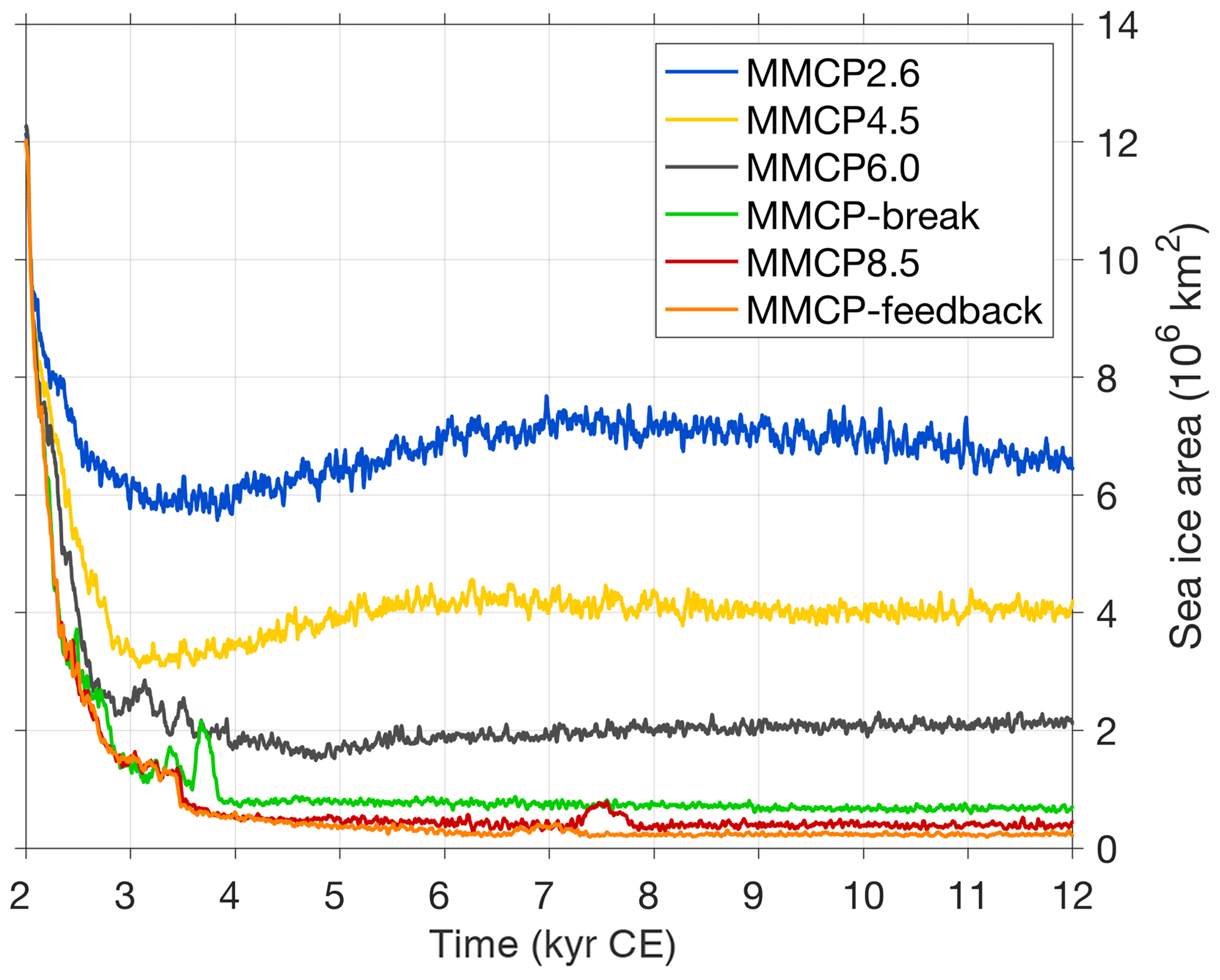
Figure 3Mean sea-ice area evolution in the Southern Ocean for the six different forcing scenarios.

Figure 4Summer insolation at 70∘ N (June) and 70∘ S (December) from 130 kyr ago at the onset of the last interglacial to the next 50 kyr. The period of our study is highlighted with vertical red lines.
4.2 The steric component
The steric component of GMSL change shows an increase following global mean temperature perturbations with the longer response time for the higher-forcing scenarios. Steric sea level rises rapidly before showing a period of stabilization for all scenarios. Except for scenarios MMCP2.6 and MMCP4.5, this period is followed by another more gradual increase in sea-level rise during the second half of the simulations (Fig. 5). This is most pronounced for scenarios MMCP6.0 and MMCP-break, where the steric contribution to GMSL rise reaches 0.3 and 0.4 m respectively between 7000 CE and 12 000 CE. Oceanic temperatures have already equilibrated to the forcing, and at 12 000 CE, deep ocean temperatures are slightly lower than temperatures at 7000 CE, following the slow decrease in global mean temperature anomalies (Fig. 6). Therefore, we attribute the sea-level rise during the second half of the simulations to the continued freshwater release from the Antarctic ice sheet. On the other hand, the steric contribution to GMSL slightly decreases for scenarios MMCP2.6 and MMCP4.5 after a peak at 3000 CE. Freshwater fluxes are still high due to a slow melting of the GrIS, suggesting that the lower increase in global mean temperatures decreases the response time. At the end of the simulations, the total range of the steric component to GMSL change is between 0.4 (MMCP2.6) and 3 m (MMCP-feedback).
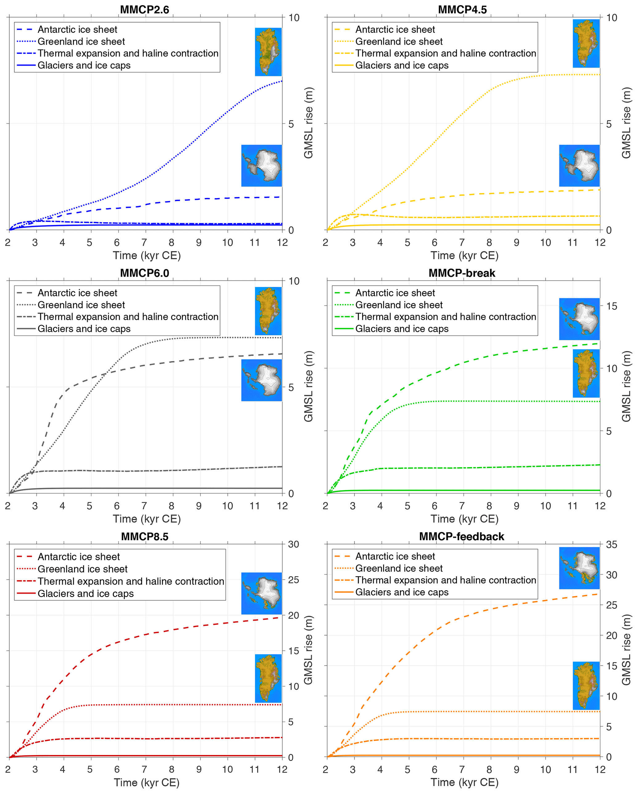
Figure 5The contribution of the different components to GMSL rise during the next 10 000 years for each of the forcing scenarios. The ice sheet geometry of Greenland and Antarctica is shown at the end of the simulations.

Figure 6Ocean temperature anomaly across the Atlantic ocean using scenario MMCP2.6 at 2100 CE (a), 2300 CE (b), 7000 CE, and (c), 12 000 CE (d) and using scenario MMCP-feedback at 2100 CE (e), 2300 CE (f), 7000 CE (g), and 12 000 CE (h).
4.3 The Greenland ice sheet and the AMOC
The GrIS volume changes because of an imbalance between the surface mass balance (SMB), i.e. the difference between accumulation and ablation, and iceberg calving at the ice sheet margin. Surface runoff is projected to increase for all the forcing scenarios, though the magnitude differs significantly. After 4000 years, surface runoff exceeds accumulation and the surface mass balance becomes negative even for the lowest forcing scenario (Fig. 7c). In scenario MMCP-feedback, this might happen already at the end of the 21st century (Fig. 7d). When looking at all the mass balance components, one can see that the relative importance of iceberg calving decreases when the ice sheet retreats on land. The large amounts of meltwater result in a total freshwater flux anomaly of 0.03 to 0.05 Sv for the three higher-forcing scenarios and are sustained for 1000 to 1500 years (Fig. 8a). The AMOC almost completely shuts down for the two highest-forcing scenarios (Fig. 9). This results in a local cooling south of the GrIS and a delayed peak warming above the Greenland ice sheet (most pronounced for MMCP-feedback; Fig. 2c), pointing to the importance of simulations with a coupled ocean–atmosphere–ice-sheet model. The AMOC recovers again after the ice sheet has melted entirely and even becomes stronger for the higher-forcing scenarios (Fig. 10).
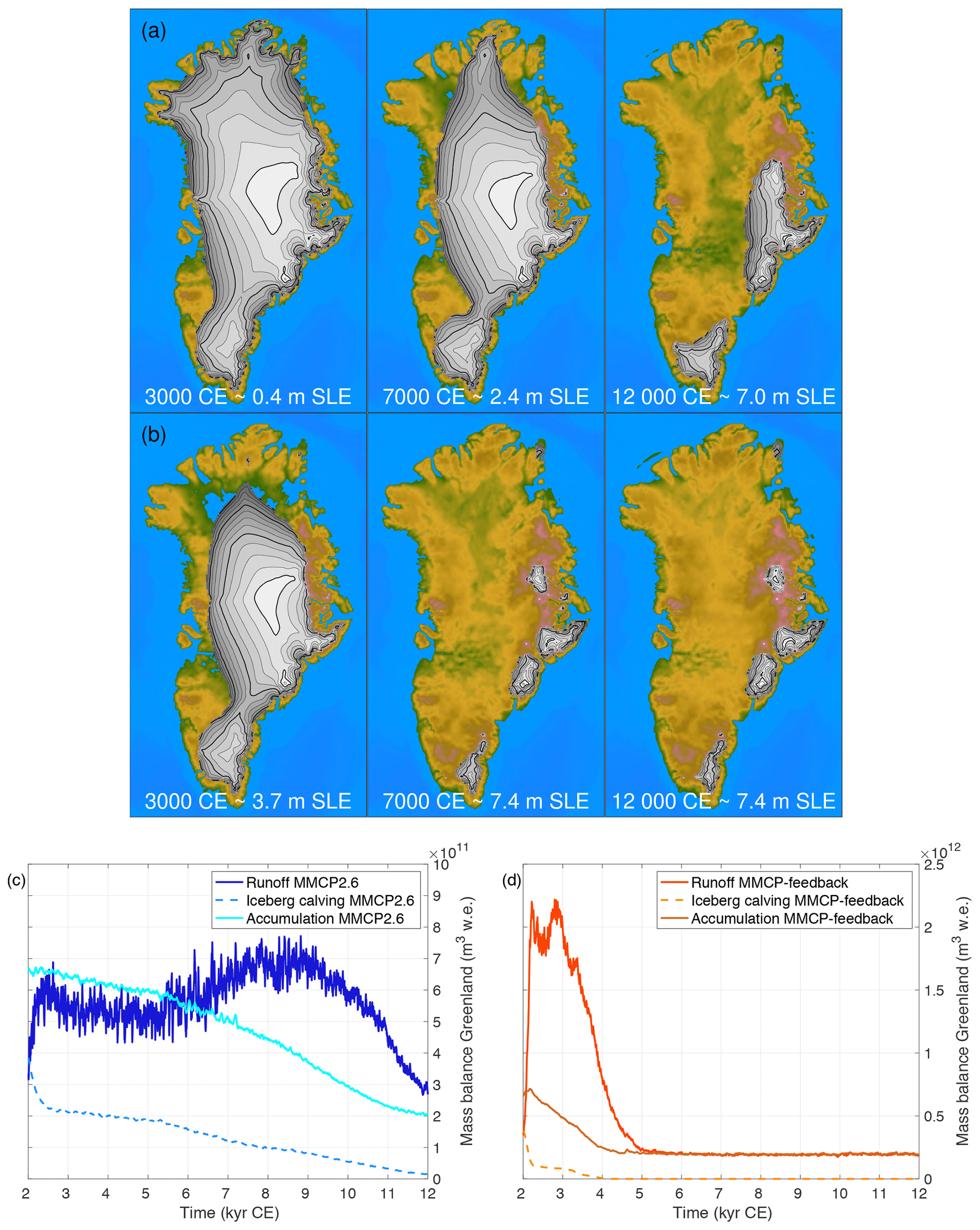
Figure 7(a) Greenland ice sheet configuration at 3000 CE, 7000 CE, and 12 000 CE using scenario MMCP2.6 and (b) MMCP-feedback. Main mass balance components explaining the change in ice sheet geometry for scenarios MMCP2.6 (c) and MMCP-feedback (d). Note that the land–sea mask has not changed due to the change in GMSL but only due to isostatic changes.
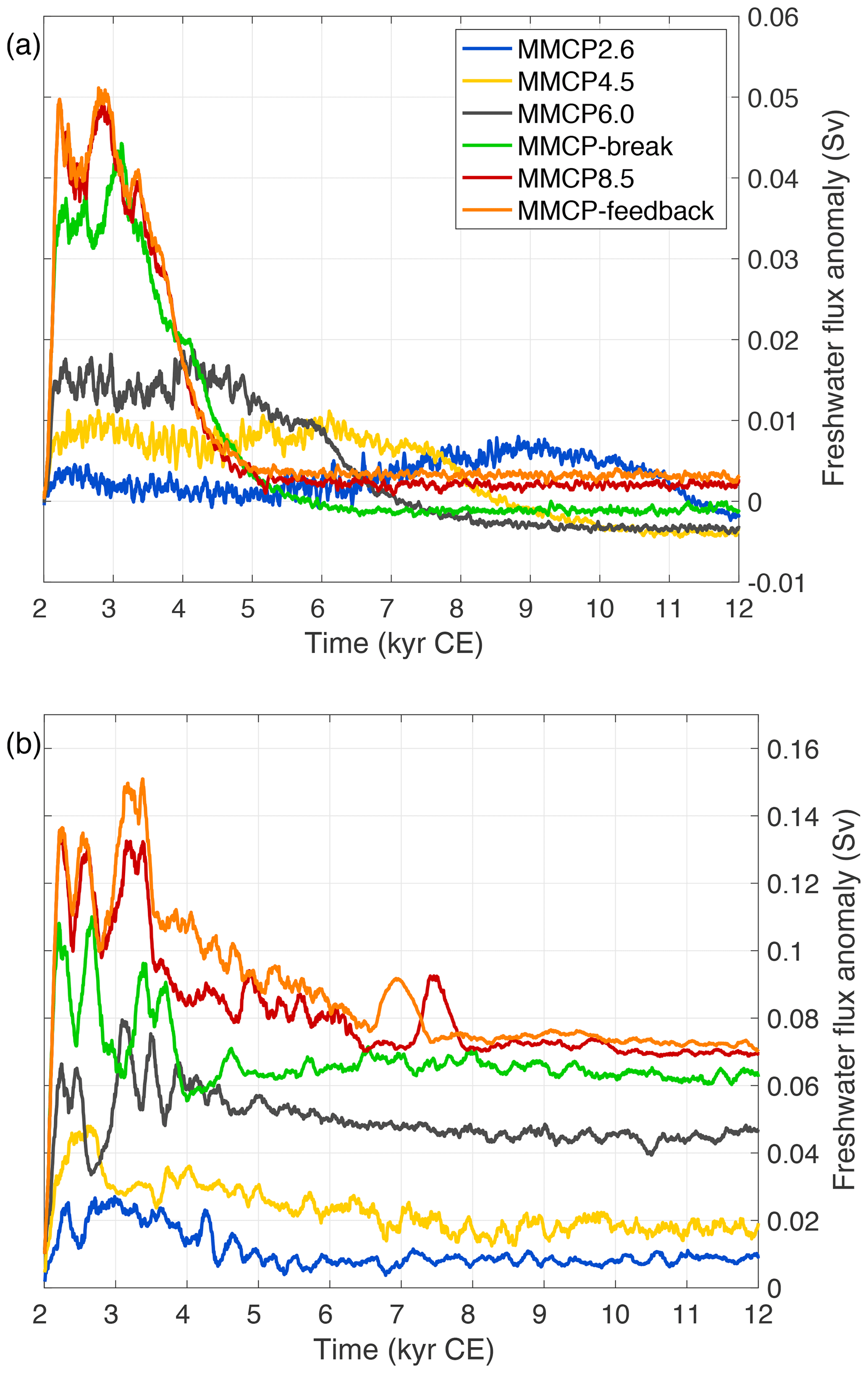
Figure 8Freshwater flux anomalies with respect to 1970–2000 from (a) the Greenland ice sheet and (b) the Antarctic ice sheet for the six different forcing scenarios.
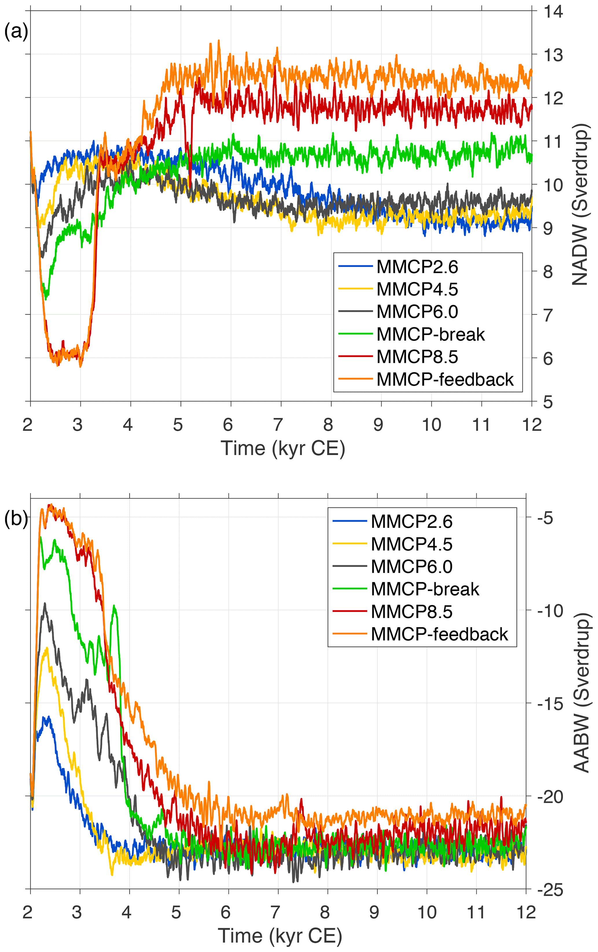
Figure 9Mean annual strength of the North Atlantic Deepwater (NADW) (a) and the Antarctic Bottom Water (AABW) (b) formation from 2000 CE to 12 000 CE. AABW is defined as the maximum of the global meridional overturning streamfunction in the bottom cell and NADW as the maximum of the meridional overturning circulation in the Greenland, Iceland, and Norwegian seas.
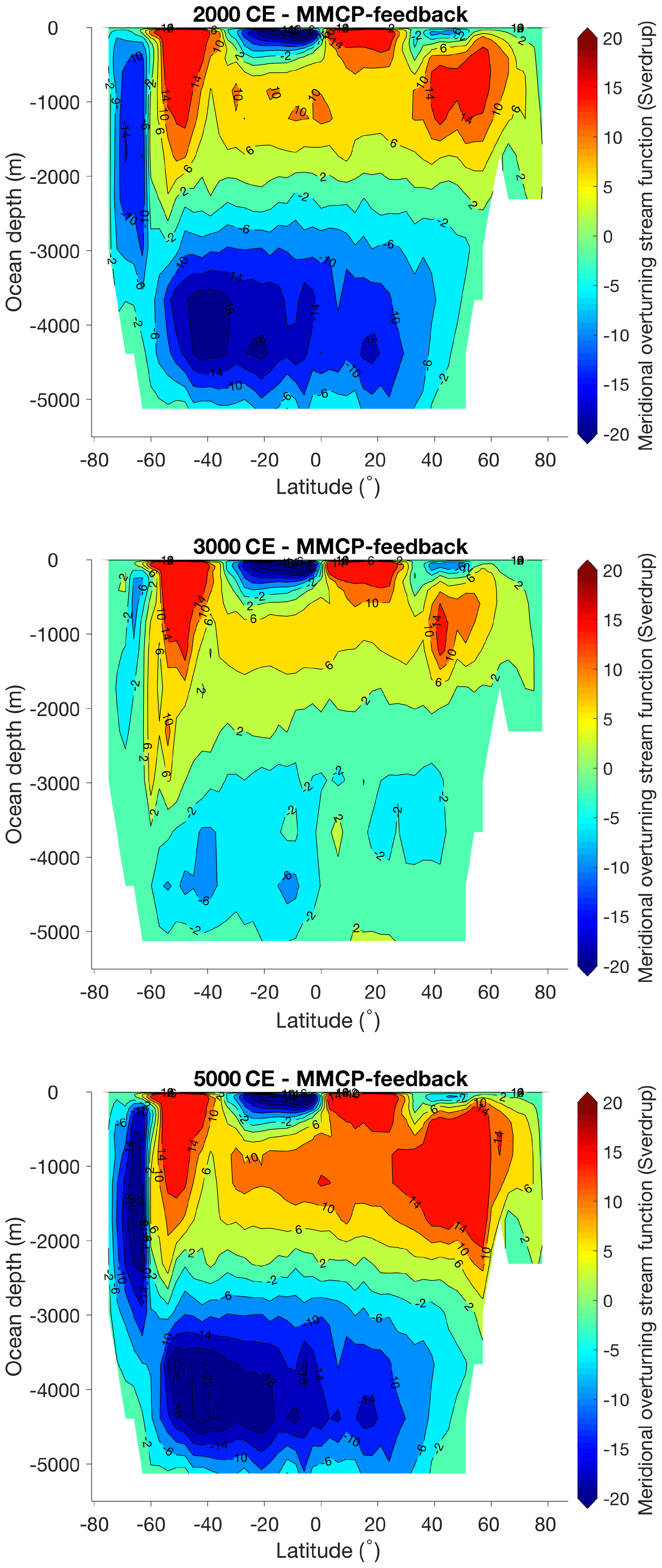
Figure 10Meridional overturning stream function for the global ocean at 2000 CE, 3000 CE, and 5000 CE using forcing scenario MMCP-feedback.
4.4 The Antarctic ice sheet and AABW
The Antarctic continent is very cold, and there is almost no surface melt over the grounded ice at present. There is a very distinct response of the AIS to a low or a high forcing in terms of mass loss. Looking at the two extremes, ice discharge at the grounding line is projected to increase slightly for scenario MMCP2.6, similar to previous suggestions that increased ice discharge is a response to increased accumulation (Winkelmann et al., 2012). The ice shelves thin for 1700 years because of atmospheric warming, while basal melting rates below the ice shelves remain low with a mean value of 0.3 m yr−1 over all the ice shelves. The ice shelves lose two-thirds of their volume, but they recover again to reach their initial volume after 5000 years when surface ablation becomes negligible. In scenario MMCP-feedback, even the large ice shelves around Antarctica disappear nearly completely after 300 years as a combination of atmospheric warming (and subsequent surface ablation) and a quadrupling in ice shelf basal melt rates. Ice discharge across the grounding line is projected to increase for about 500 years and drops below present-day values after 1700 years when the West Antarctic Ice Sheet has collapsed and the East Antarctic Ice Sheet starts to retreat land inwards. The increase in surface runoff is even stronger and exceeds accumulation at the end of the first millennium for about 3000 years, after which surface runoff and ice discharge along the grounding line stabilize and account each for about half of the mass loss (Fig. 11d). The freshwater input in the Southern Ocean increases with 0.14 Sv for the highest-forcing scenario and remains elevated until the end of the simulations with an anomaly of 0.07 Sv due to continued ice sheet melting and increased runoff over land (Fig. 8b). As a consequence of the freshwater release into the Southern Ocean, the strength of AABW declines with 23 % for MMCP2.6 and up to 77 % for MMCP-feedback during the next 500 years due to rapid ice sheet melting (Fig. 9b). These freshwater fluxes from the AIS lead to reduced oceanic warming in the vicinity of Antarctica and relatively low basal melt rates in our experiments (mean basal melt rates of 0.5–1.1 m yr−1 for scenario MMCP-feedback during the coming centuries). Mean SAT anomalies above the Antarctic ice sheet reach a maximum between 5000 and 6000 CE when the ice sheet retreats on land and the albedo–temperature feedback sets in (Fig. 2d). The mass balance components stabilize during the second half of the simulations with iceberg calving and ablation both accounting for half of the mass loss, a situation comparable to the Greenland ice sheet today.
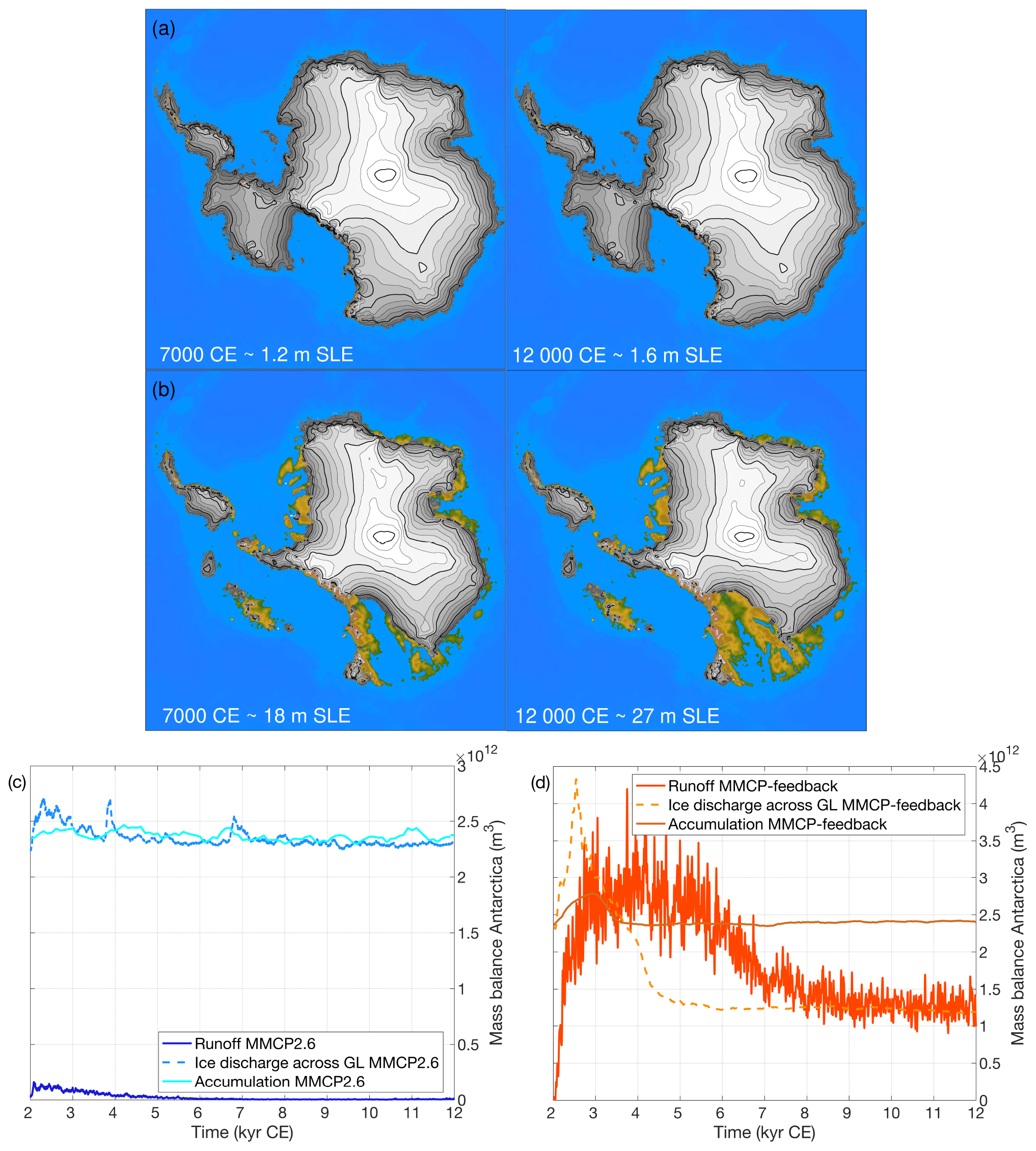
Figure 11(a) Antarctic ice sheet configuration at 7000 CE and 12 000 CE using scenario MMCP2.6 and (b) MMCP-feedback. Only grounded ice is shown. Main mass balance components (over grounded ice) explaining the change in ice sheet geometry for scenarios MMCP2.6 (c) and MMCP-feedback (d). GL: grounding line. Note that the land–sea mask has not changed due to the change in GMSL but only due to isostatic changes.
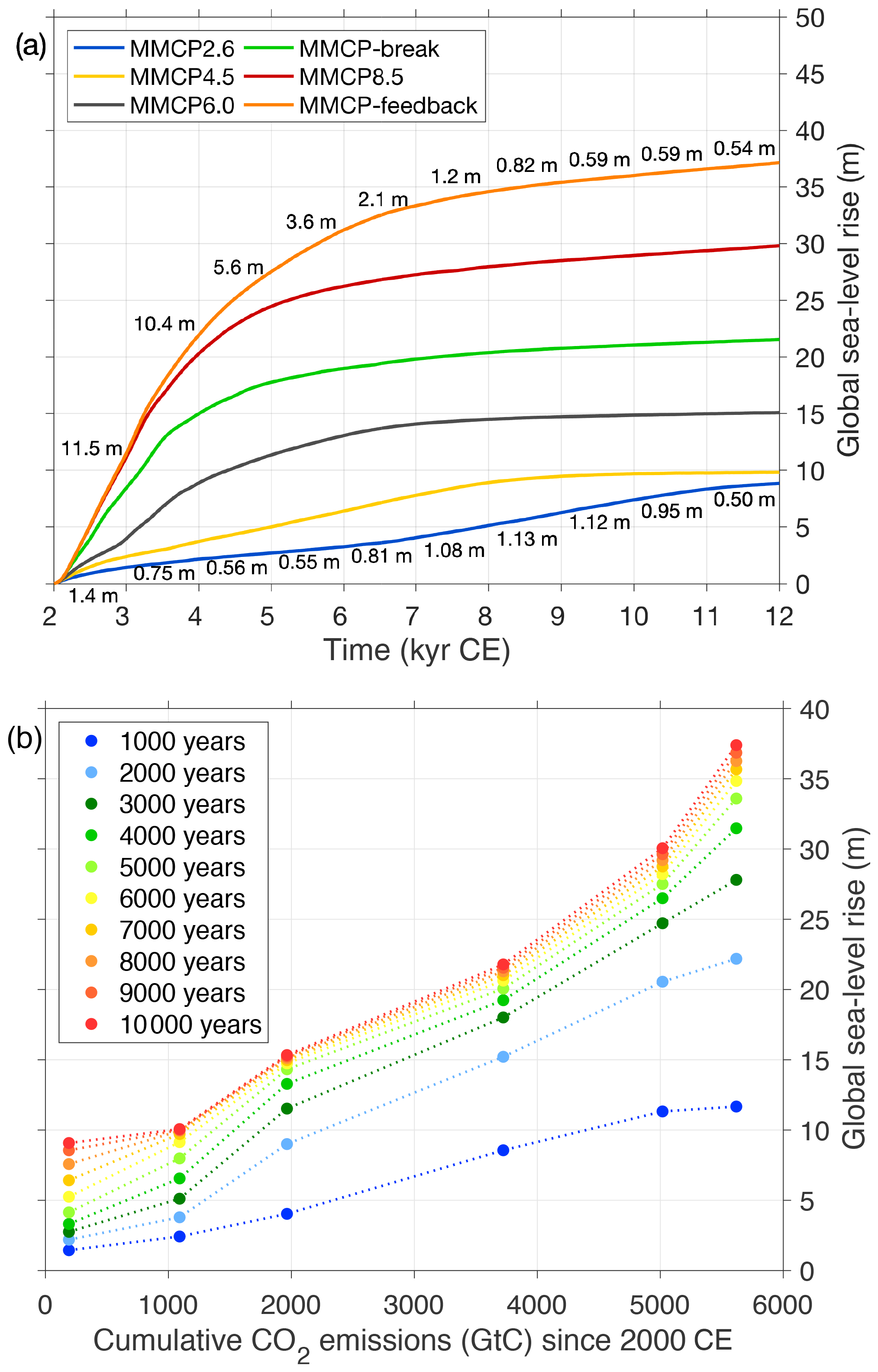
Figure 12(a) GMSL rise as the sum of the contributions from the AIS, the GrIS, glaciers and ice caps, and the steric component. The rate of sea-level rise during each millennium is indicated for the lowest and highest scenarios. (b) GMSL rise for a given cumulative CO2 emission at the end of each millennium until 12 000 CE.
There is a very large difference in ice sheet geometry of the AIS after 10 000 years for the lowest- and highest-forcing scenario. In scenario MMCP2.6, the grounding line retreats mostly in the Weddell Sea and the Ross Sea basin, with almost no retreat for the East Antarctic Ice Sheet (Fig. 11a). For the high emission pathway, the West Antarctic Ice Sheet collapses and grounding line retreat initiates in the Wilkes subglacial basin (Fig. 11b). Due to isostatic rebound of the Earth's crust, more land is exposed above sea level at 12 000 CE compared to the situation at 7000 CE and the ice sheet margin becomes land-based for most of East Antarctica as has been proposed for warm intervals during the mid-Miocene (Gasson et al., 2016; Frigola et al., 2018).
4.5 Glaciers and ice caps
Glaciers and ice caps have a decadal to century timescale response and are vulnerable to small perturbations in the climate forcing. For the highest-forcing scenarios MMCP-break, MMCP8.5, and MMCP-feedback, the glaciers and ice caps melt away entirely in the coming 1000 to 2000 years. Under scenario MMCP2.6 it takes up to 3000 years before the glaciers and ice caps lose most of their ice volume. On the multi-millennial timescale, the differences in the glaciers' and ice caps' contribution to sea-level change are very small compared to the other components with total contributions between 0.23 and 0.24 m for any of the forcing scenarios.
Total GMSL changes in our experiments range between 9.2 and 37.4 m at the end of the 10 000 year experiments (Fig. 12a). Moreover, the rates of GMSL rise vary substantially between the different scenarios and over time. We investigate the relation between cumulative CO2 emissions and GMSL change, somewhat similar to the notion of a relationship between global warming and cumulative CO2 emissions by a certain time, expressed as the transient climate response to cumulative carbon emissions (TCRE; Matthews et al., 2018) or the multi-millennial climate response to cumulative carbon emissions (MCRE; Frölicher and Paynter, 2015). In Fig. 12b, the realized GMSL rise after each 1000 years is shown as a function of the total cumulative CO2 emission after 2000 CE for each experiment.
In the case of total cumulative CO2 emission exceeding 2000 GtC, GMSL change rates are highest during the first 2 millennia. However, when cumulative CO2 emissions stay below 200 GtC (MMCP2.6), the peak rates in GMSL change occur only 4000 to 8000 years from now due to slow melting of the GrIS and ensuing feedbacks. A total sea-level rise of 9.2 m is achieved after 10 000 years, even though CO2 emissions already ceased before the mid-21st century. For the other experiments, the rate of sea-level change decreases with time. All experiments approach a semi equilibrium after 10 000 years (Fig. 12a). The rate of global sea-level change is then still positive for all simulations, albeit reduced to about 0.05 m per century for the experiment with the largest cumulative CO2 emission (MMCP-feedback). This reflects the long equilibration time for the ice sheets and the ocean within the coupled climate system to adapt to temperature changes.
In our simulations, Greenland is the largest contributor to GMSL rise up to a cumulative CO2 emission of 2000 GtC. The grounding line of the West Antarctic Ice Sheet (WAIS) retreats several 100 km inland using scenario MMCP2.6 and MMCP4.5. The WAIS disintegrates completely for cumulative CO2 emissions around 2000 GtC, but East Antarctica still remains mostly unaffected. For higher cumulative emissions, marine-based parts of East Antarctica start to disintegrate and Antarctica becomes the largest source for GMSL rise.
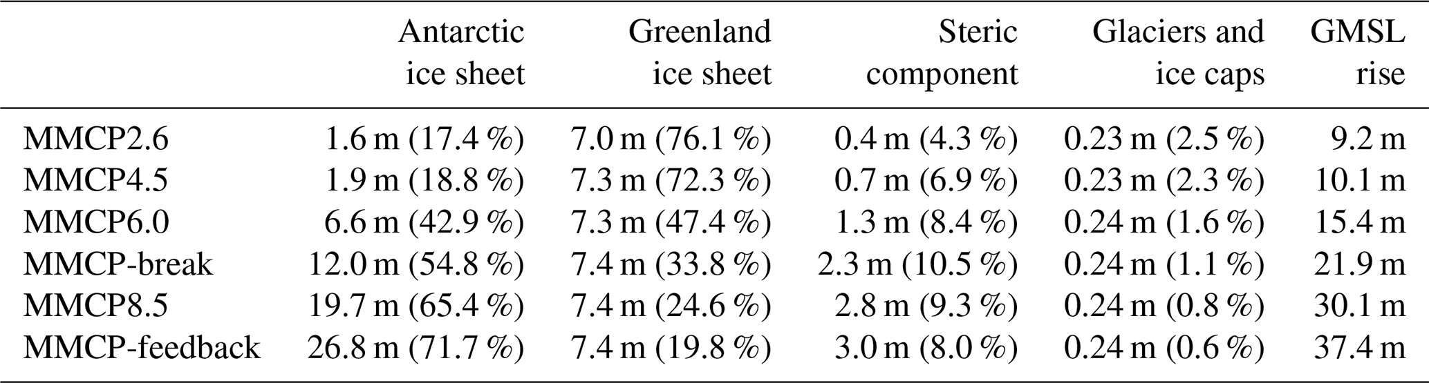
The total sea-level rise at 12 000 CE includes the (nearly) entire melt of the Greenland ice sheet as well as glaciers and ice caps. The spread is largest for the Antarctic contribution taken over all scenarios, ranging from 1.6 to 27 m (corresponding to ∼200 to ∼5000 GtC cumulative CO2 emissions after 2000 CE). The steric contribution ranges between 0.4 and 3 m. Table 1 gives an overview of the sea-level contribution and the relative share to GMSL of each component for all forcing scenarios.
Table 1Sea-level contribution from the different components contributing to GMSL change for scenarios MMCP2.6, MMCP4.5, MMCP6.0, MMCP-break, MMCP8.5, and MMCP-feedback, shown in metres and as a percentage of GMSL change.
The uncertainty in the future sea-level change projections, related to the climatic parameters in LOVECLIM, is evaluated by running the coupled model for three different climatic parameter combinations (P32a, P22, and P11). As explained in the model description, the main difference is denoted by the first digit and represents a measure of the model climate sensitivity (CS) where the CS is largest for P32a and lowest for P11 (more information on the parameter differences can be found in the Supplement). There is limited model uncertainty in GMSL change during the next 10 000 years for the lowest-forcing scenario MMCP2.6. GMSL rise ranges between 7.5 m for parameter set P11 to 9.2 m for parameter set P22. For scenario MMCP-feedback, the range in GMSL rise is very large going from about 19.9 m for parameter set P11 to 77.0 m for parameter set P32a (Fig. 13). The maximum sea-level rise consists of a contribution of 63 m from the AIS, 7.3 m from the GrIS, 5.8 m from the steric component, and 0.24 m from glaciers and ice caps. Note that the contribution of 63 m from the AIS is more than the estimate of 58 m SLE stored in the AIS volume (Fretwell et al., 2013) due to the inclusion of bedrock elevation changes after isostatic unloading and its influence on sea-level rise (Goelzer et al., 2020a).
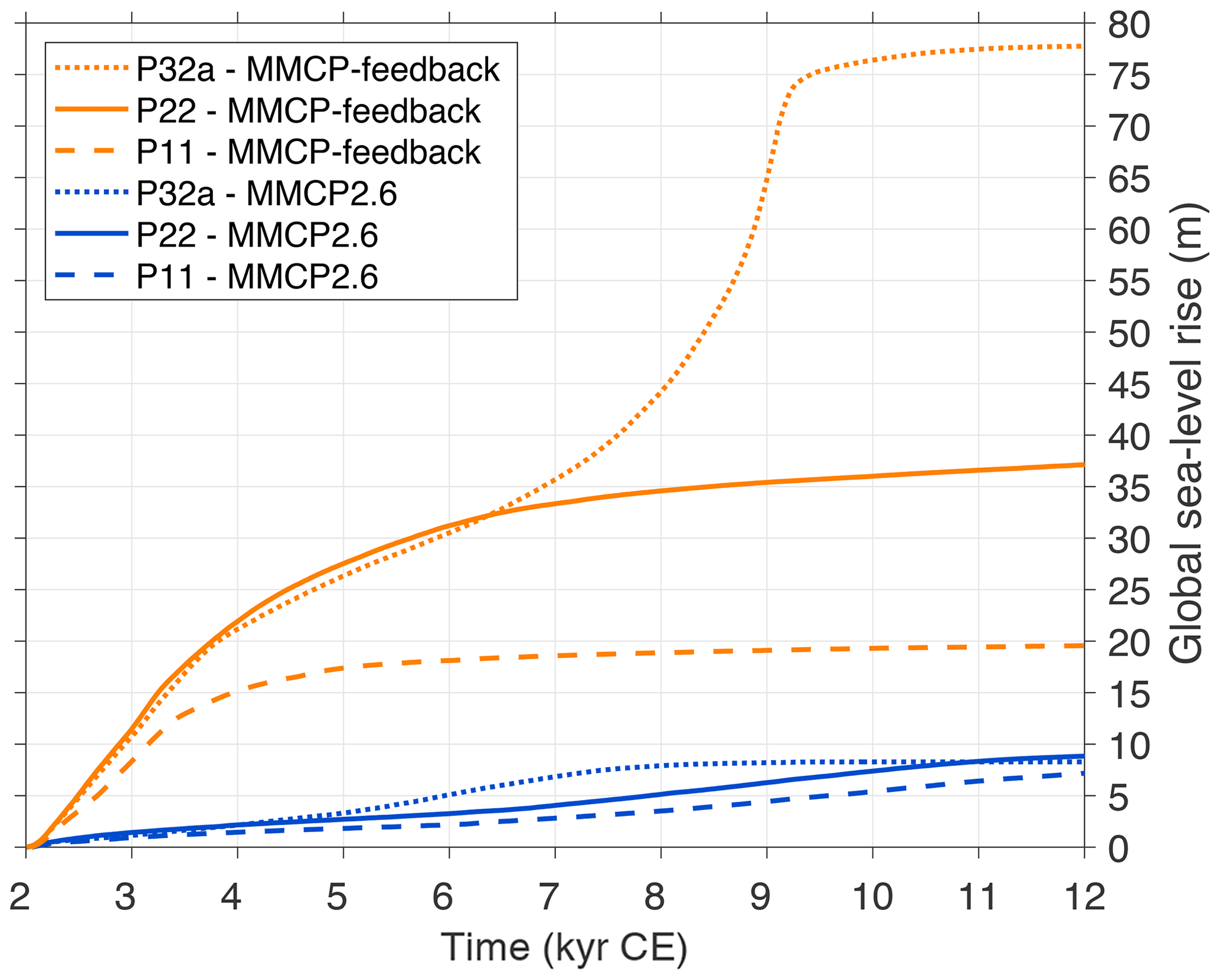
Figure 13Global sea-level rise for three different climatic parameter sets of LOVECLIM using forcing scenario MMCP2.6 and MMCP-feedback. GMSL change from our preferred parameter set P22 is given in solid lines.
The large uncertainty that arises using scenario MMCP-feedback comes mainly from the AIS. Especially the acceleration in GMSL using parameter set P32a is remarkable, where the fastest rates in sea-level rise occur around 7000 years from now. In this experiment, a very strong albedo–temperature feedback initiates once a significant part of the ice sheet retreats on land. The ice melts at a rate of 30 m SLE in 1500 years. This freshwater input is even larger than meltwater pulse 1A around 14.6 ka BP, where the global meltwater input is estimated to have been between 14 and 25 m in 400–500 years (Cronin, 2012), albeit in a situation where initially 3 times more ice volume was present.
An interesting test for our sea-level change projections can be provided by the geological record of sea-level high stands as a function of the reconstructed atmospheric carbon dioxide concentration. Estimates of paleo sea-level variations range from a lowstand of −120 m for CO2 concentrations around 180 ppmv during glacial intervals of the Quaternary to a highstand of +65 m for CO2 concentrations up to 1200 ppmv during the Eocene (Alley et al., 2005; Foster and Rohling, 2013). Such data suggest a linear sigmoidal behaviour for (semi)-equilibrated periods in the past, where sea-level high stands change abruptly for deviations in the greenhouse gas forcing from the pre-industrial period due to the build-up of the large Northern Hemisphere ice sheets during glacial periods and the total melting of the Greenland and Antarctic ice sheets for a high-CO2 greenhouse world during the Eocene (Fig. 14). Assuming that our climate (and sea-level change) components are nearly equilibrated after 10 000 years, we compare our GMSL changes with the geological archive (Foster and Rohling, 2013). For this comparison, it is important to realize that the timescale of carbon input in the atmosphere may be a critical parameter as the peak atmospheric CO2 concentration shows a strong dependence on the emission pathway. However, simulations with biogeochemical models show that the mean atmospheric CO2 concentration over multiple kiloyears is mostly independent of the duration of carbon release (Zeebe and Zachos, 2013). Moreover, on a multi-centennial timescale, global mean temperature perturbations converge to a single value, suggesting a pathway independence of cumulative emissions (Zickfeld et al., 2012; Rogelj et al., 2016). We therefore opt to average the CO2 concentration over the next 10 000 years, suggesting that the mean concentration represents the multi-millennial temperature change at best.
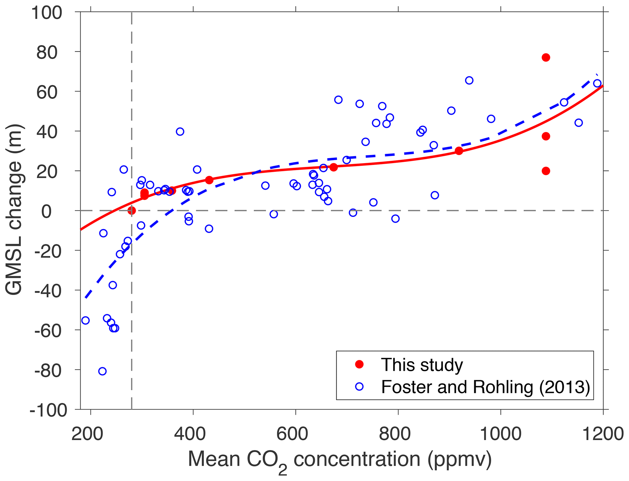
Figure 14Semi-equilibrated GMSL change projections at 12 000 CE compared to the geological record of sea-level high stands (Foster and Rohling, 2013) for a given atmospheric CO2 concentration. The atmospheric CO2 concentrations used for the projections of GMSL are averaged over the 10 000-year simulation. The horizontal line at 0 m GMSL change represents the present-day situation. For scenario MMCP2.6 and MMCP-feedback, the GMSL uncertainty is given by including the experiments with the three different climatic parameter sets. The red line is the best fit for the data from our study, while the blue line is the best fit for the Foster and Rohling (2013) data.
Figure 14 shows the GMSL change after 10 000 years as a function of the mean atmospheric CO2 compared with the geological archive. We compared the best fit of the data obtained in this paper (red line; polynomial with exponent 3) with the best fit of the geological data (blue line, polynomial with exponent 2; data from Foster and Rohling, 2013). The fitted lines compare quite well. There is a somewhat larger discrepancy for the lowest CO2 concentrations, because we do not include sea-level projections for CO2 concentrations below pre-industrial levels. The geological estimates of sea-level high stands include data that are affected by the hysteresis effect between ice sheet growth and ice sheet decay, where an ice sheet can either exist or not exist at a certain CO2 level depending on its history (Pollard and DeConto, 2005). In this regard, higher CO2 values are needed to melt ice sheets than to make them grow. Also the effect of a different paleotopography might have had an influence on the inception of ice on paleo timescales where the AIS could grow for higher CO2 values during the Oligocene than at present due to the higher bedrock topography (Paxman et al., 2019). Both arguments suggest that our curve (red line) is expected to be below the best estimate of the geological data (blue line), requiring higher CO2 levels to melt the ice sheets on Earth in the future than during periods in geological history.
Glaciers and ice caps are the second-largest contributor to present-day GMSL rise (after the thermosteric component) and will continue to be a major source of sea-level rise during the next century (Huss and Hock, 2015; Hock et al., 2019; Marzeion et al., 2020). At the end of the 21st century, the global glacier volume is projected to decrease by between 21 % (MMCP2.6) and 24 % (MMCP8.5) of its current value. The contribution to GMSL from glaciers and ice caps melting generally corroborates the findings by Hock et al. (2019), who found that by the end of the 21st century mountain glaciers and ice caps lose between 11 %–25 % (RCP2.6) and 25 %–47 % (RCP8.5) of their volume. For scenario MMCP8.5, our results are below the average estimates at the end of the 21st century because of the rather low climate sensitivity in LOVECLIM. At the end of the simulations, the lower sensitivity of our glacier model to the high-forcing scenarios is irrelevant, and glaciers and ice caps will lose 96 %–100 % of their volume for any of the forcing scenarios. Raper and Braithwaite (2006) and Goelzer et al. (2012) found that glaciers and ice caps disappear completely for a global warming of around 4 ∘C by the end of the third millennium.
The steric sea-level contribution has a sensitivity of between 0.27 and 0.68 m ∘C−1 in our study, where the stronger forcing scenarios have the higher contribution due to the additional effect of haline contraction. Levermann et al. (2013) identified a similar linear relation between thermal expansion and global mean temperatures of 0.2 to 0.63 m ∘C−1. Hieronymus (2019) assessed several coupled climate models that include ocean circulation changes and found an updated sensitivity of 0.51 to 0.83 m ∘C−1 of surface warming. The higher sensitivity is present in climate models that show an increase in AMOC strength. However, the AMOC strength (temporarily) decreases in our experiments, especially in the simulations where the GrIS is melting fast. Therefore, the higher sensitivity reported by Hieronymus (2019) might be an overestimation in future scenarios where the ice sheets will melt strongly, due to the neglection of ice-sheet–ocean interactions.
The largest (scenario-based) uncertainty in future multi-millennial sea-level rise comes from the polar ice sheets. In our simulations, the melting of the entire GrIS takes about 10 000 years for a mean SAT anomaly of 2 ∘C with respect to 1970–2000 CE. In higher scenarios, the GrIS needs between 8000 years for MMCP4.5 with a mean SAT anomaly of 5.1 ∘C and 2000 years for MMCP-feedback with a mean SAT anomaly of 9.8 ∘C, to disintegrate entirely. Robinson et al. (2012) found the temperature threshold for melting the entire Greenland ice sheet to lie between 0.8 and 3.2 ∘C, with a long decay time for temperatures close to this threshold. Since the temperature anomaly in scenario MMCP2.6 is close to this threshold, it takes about 10 000 years in our simulations to melt the entire GrIS. According to Aschwanden et al. (2019), the GrIS will lose between 72 % and 100 % of its volume by the end of the next millennium, using an extreme melt forcing and neglecting the temporary cooling effect of a reduced AMOC. Other studies found that the GrIS could disappear in less than 3000 years for a constant CO2 forcing exceeding 1100 ppmv (Alley et al., 2005; Driesschaert et al., 2007; Huybrechts et al., 2011), in the same range as our simulations even though the results are not entirely comparable owing to a different time evolution of the CO2 and temperature forcing.
The AMOC in LOVECLIM exhibits a monostable behaviour where the recovery to the initial state starts as soon as the meltwater pulse halts. An EMIC intercomparison study found that seven models show a bistable regime and four others a monostable regime following a freshwater perturbation in the North Atlantic (Rahmstorf et al., 2005). A monostable regime of the AMOC is simulated in most GCMs where a freshwater pulse leads to a temporary reduction in the AMOC strength and a recovery when the freshwater pulse terminates (Liu et al., 2014). However, it is speculated that a monostable regime might be caused by a negative salinity bias in GCMs (Mecking et al., 2017) and that a bistable regime would explain the rapid climatic changes during the deglaciation better (Ganopolski and Rahmstorf, 2001). The equilibrium response of the ocean suggests that the AMOC strength will also increase in response to atmospheric warming, possibly due to a decrease in sea-ice area (Jansen et al., 2018). Several studies found that the AMOC was also stronger during the mid-Pliocene, in the absence of freshwater feedbacks due to ice sheet melting (Chandan and Peltier, 2017; Chan and Abe-Ouchi, 2020). Our study supports the increase in the AMOC strength when the freshwater forcing halts.
The marine-based WAIS is considered the most vulnerable part of the AIS and collapses for cumulative CO2 emission exceeding ∼1100 GtC. The Wilkes subglacial basin in East Antarctica becomes ice-free in scenarios MMCP-break, MMCP8.5, and MMCP-feedback. The Aurora Basin also loses its ice cover for scenario MMCP-feedback. The ice sheet respectively contributes 12, 19.6, and 27 m to sea level following scenarios MMCP-break, MMCP8.5, and MMCP-feedback (Fig. 5). Our numbers for MMCP8.5 are comparable to the study by Golledge et al. (2015), equally based on an extension of the ECP8.5 scenario with constant forcing after 2300 CE. They found that AIS retreat over the Wilkes and Aurora basins would contribute up to 11.4 m to GMSL after 5000 years and 15.7 m after 50 000 years. In the simulations of Winkelmann et al. (2015), the grounding line retreats significantly along the WAIS for a cumulative emission of 1000 GtC, while in East Antarctica the retreat is most rapid for the Wilkes and Aurora subglacial basins and initiates for a cumulative CO2 emission of 2500 GtC. Considering a cumulative CO2 emission of 10 000 GtC, Winkelmann et al. (2015) even found that the Antarctic ice sheet could nearly disappear entirely. However, that is an extreme scenario at the upper end of potential carbon reserves and resources available for combustion, which we did not consider in the present paper.
Even though the resolution of the ice sheet models and the climate model is relatively coarse, especially to simulate the retreat along the outlet glaciers in Greenland and the grounding line retreat in the most sensitive Antarctic regions such as Thwaites or Pine Island glaciers in West Antarctica, we have confidence that the model is performing quite well to simulate the ice sheet response on the millennial timescale. Marine-terminating glaciers along the Greenland ice sheet will retreat in the coming decades and the SMB will dominate the Greenland mass loss. The Antarctic ice sheet model run at 20 km resolution is too coarse to simulate fast-flowing glaciers in great detail, and the omission of sub-grid scale mechanisms makes the model less sensitive in the short term to basal melting (Levermann et al., 2020, Seroussi et al., 2020). However, the grounding line retreats on land in Antarctica for most scenarios and also here, the influence of SMB processes becomes more important. Because of the rather low contribution of the AIS to sea-level by 2300 CE for scenario MMCP2.6 and the lower sensitivity to grounding line retreat compared to other ice sheet models (Levermann et al., 2020), we assume that our lowest sea-level change value is a conservative estimate.
It should be noted that our ice sheet models do not include hydrofracturing. Hydrofracturing may significantly speed up Antarctic ice sheet decay as achieved by the marine ice cliff instability (MICI) mechanism (Pollard et al., 2015). DeConto and Pollard (2016) find Antarctic ice sheet volume losses equivalent to a freshwater input into the surrounding ocean in excess of 1 Sv, much larger than the peak freshwater input in our simulations of 0.15 Sv. However, the MICI is controversial for its large contribution to sea level already at the end of the 21st century (e.g. Edwards et al., 2019).
Clark et al. (2016) found the AIS to be the largest contributor to sea-level rise after 10 000 years for all of the scenarios they considered. Moreover, it is suggested that the sensitivity of GMSL change to atmospheric CO2 decreases for higher cumulative CO2 emissions with a logarithmic relation between both. For the first 2 millennia, our results show a similar behaviour, but at the end of the 10 000-year simulations, GMSL increased more for the higher-emission scenarios, and a stronger non-linear relationship between GMSL and cumulative CO2 emissions was established. Part of the discrepancy can be explained by the difference between scenario MMCP8.5 and MMCP-feedback. Both scenarios assume the same peak CO2 values, but the latter adds more carbon to the atmosphere after 10 000 years due to the methane emission feedback. Another difference with our experiments is that we include the albedo–temperature feedback, which gains importance once the Antarctic ice sheet retreats inland.
Oppositely to previous modelling studies investigating the Antarctic ice sheet evolution on a multi-millennial timescale (Winkelmann et al., 2015; DeConto and Pollard, 2016; Clark et al., 2016), we include the two-way feedbacks between the ice sheets, the atmosphere, and the ocean. Large amounts of freshwater – due to the melting of the ice shelves and grounded ice from Antarctica – enter the Southern Ocean and impact on Antarctic Bottom Water (AABW) and sea-ice formation (Swingedouw et al., 2008; Goelzer et al., 2016a, b). On the other hand, freshwater fluxes from melting the GrIS strongly reduce the North Atlantic Deepwater (NADW) formation and weaken the AMOC. The interhemispheric see–saw effect is understood as weakening NADW formation, leading to a reduced transport of cold water to the Antarctic leading to a warming of the Antarctic continent (Stocker, 1998). However, in our future warming simulations, the AIS is also melting and freshwater fluxes act as a negative feedback by limiting the ocean temperature increase locally. The observed limited warming in our simulations is supported by a study from Swingedouw et al. (2009), who found regional cooling of up to 10 ∘C following a freshwater release of 1 Sv in the Southern Ocean. In contrast, other studies suggest an increase in sea-ice area due to large freshwater pulses (Swingedouw et al., 2008; Goelzer et al., 2016b) where the ocean stratification increases beneath the ocean surface leading ultimately to ice shelf melting at depth (Golledge et al., 2014). This positive feedback is not observed in our simulations, where the sea-ice area (and volume) declines strongly in all our experiments and almost all sea ice disappears for the three highest-forcing scenarios at the end of the first millennium (Fig. 3).
In this paper we have assessed multi-millennial sea-level change projections having fully interactive ice sheet components as obtained within the Earth system model of intermediate complexity LOVECLIM. Global mean sea level is shown to continuously rise during the next 10 000 years for all scenarios considered. These build further on IPCC RCP/ECP scenarios with emission pathways ranging from temporarily negative emissions to burning ∼5000 GtC with the addition of a methane emission feedback. Using the RCP-based scenarios, our sea-level change projections are found to be irreversible on a 10 000-year timescale, even for the lowest-forcing scenario based on extending scenario RCP2.6/ECP2.6 with zero emissions.
The interactive nature of our model study on the multi-millennial timescale is important to simulate most climatic feedbacks in an accurate way. Ice-sheet–ocean interactions result in temporarily large perturbations in the ocean circulation with freshwater fluxes from the GrIS leading to a strongly reduced AMOC strength and local cooling. Apart from the local cooling effect and its influence on atmospheric temperatures in the vicinity of the Greenland ice sheet, our findings suggest that the reduced AMOC also lowers the contribution from the steric component to GMSL. Freshwater fluxes from the AIS lead to reduced oceanic warming in the vicinity of Antarctica and relatively low basal melt rates. Ice-sheet–atmosphere interactions on a multi-millennial timescale are important to take into account because of the SMB–elevation feedback that sets in when the ice sheet starts to melt and the surface elevation decreases. The strong albedo–temperature feedback initiates when the ice sheets retreat on land, where temperatures increase due to an increase in the tundra-like surface type (in addition to the effect of a reduced sea-ice area). As a consequence, surface melting accelerates once a critical area of land becomes ice-free.
It is found that the Greenland ice sheet will melt entirely over the next 10 000 years, but the rate of sea-level rise is determined by the forcing scenario. Oppositely, the fate of the Antarctic ice sheet is largely dependent on the future greenhouse gas forcing scenario considered. For the lowest forcing scenario, there is only a limited retreat of the grounding line in West Antarctica and the East Antarctic Ice Sheet remains mostly unaffected, resulting in a limited sea-level contribution of 1.6 m. For the highest-forcing scenarios, the West Antarctic Ice Sheet is found to collapse entirely and there is significant marginal ice sheet retreat along the East Antarctic Ice Sheet with a total volume loss of around 27 m SLE. The steric sea-level change component continues to contribute to sea-level rise as long as there is a freshwater influx, even though the bulk of the oceanic heat increase takes place in the first centuries after the steep rise in temperatures. It is the only component contributing to sea level that reaches a peak during the coming millennia and decreases slowly towards the end of the simulations (only for the two lowest scenarios) following a slight global cooling trend after a few thousand years. Glaciers and ice caps are the smallest component in the sea-level budget and disappear relatively fast during the coming centuries.
We have identified the existence of a threshold in total cumulative CO2 emissions for which GMSL is dominated by the melting of the Greenland ice sheet or the Antarctic ice sheet. In our simulations, GMSL rise is dominated by the melting of the Greenland ice sheet for a total cumulative CO2 emission of up to 1100 GtC (after 2000 CE). Under these scenarios, GMSL is found to quasi stabilize between 9.2 and 15 m above current levels. For the higher-emission scenarios, the AIS contribution exceeds the GrIS contribution after 1000 years due to grounding line retreat and surface melting in East Antarctica, and total GMSL rise after 10 000 years ranges between 22 and 37.4 m. Near the end of the simulations, the rate of sea-level change decreases to values below 0.05 m per century for all forcing scenarios and sea-level approaches a semi-equilibrated state.
We assume that an impulse response function (IRF) represents the time-dependent abundance of a gas after an additional emission pulse (Joos et al., 2013; Maier-Reimer and Hasselmann, 1987). After the peak concentration, the CO2 concentration decreases exponentially reaching a short-term equilibrium (after 1000 years) and a long-term equilibrium (after 10 000 years) based on Eqs. (1) and (2) (Solomon et al., 2009). The time constants used for the two exponentials do not have a process-based meaning but are fitting parameters to best represent the wide range of IRFs present in the literature. The peak airborne fraction (AFpeak), the short-term stabilization level , and the long-term stabilization level (∗ can be replaced by l and s in Eq. 2) represent the different theoretical neutralization processes.
where is equilibrium CO2 concentration after 1000 years, is equilibrium CO2 concentration after 10 000 years, is peak CO2 concentration, λs is short-term decay rate, λl is long-term decay rate, and t is time (between peak concentration and 12 000 CE).
where = 280 ppmv, AF is equilibrium airborne fraction, and AFpeak is peak airborne fraction.
The instantaneous or peak airborne fraction (AFpeak) is the atmospheric CO2 peak concentration as a percentage of the total released CO2 (Archer and Brovkin, 2008). AFequi measures the fraction of emitted CO2 that remains in the atmosphere after 1000 years (AF) and 10 000 years (AF) respectively. The main principle is that the more CO2 is emitted in the atmosphere, the lower the capacity of the ocean to buffer the excess of carbon due to the limited size of the ocean (Archer et al., 2009a). Dissolved carbon in the ocean consists of bicarbonate () and carbonate ions (). The latter buffers the ocean against CO2 invasion but is less abundant than bicarbonate. Depletion of the bicarbonate ions starts with increasing atmospheric CO2 concentrations. As a consequence, the buffering capacity of the ocean decreases with higher-CO2 atmospheric injections (Archer and Brovkin, 2008).
The airborne fractions are chosen in accordance with the values present in the literature (Table A1) and extrapolated for the scenarios that do not correspond to the CO2 emission pulses (Table A2). The peak airborne fraction after a pulse injection of CO2 is 100 % and therefore not completely comparable with the more gradual injections as assumed by the MMCP scenarios. Therefore, these peak airborne fractions are scaled to the peak airborne fractions for a slower injection of CO2 where the peak atmospheric CO2 value is between 50 % and 70 % of the real atmospheric CO2 emissions (Archer and Brovkin, 2008).
Table A1Estimates of CO2 airborne fractions available in the literature 1000 and 10 000 years after a pulse of CO2 into the atmosphere.
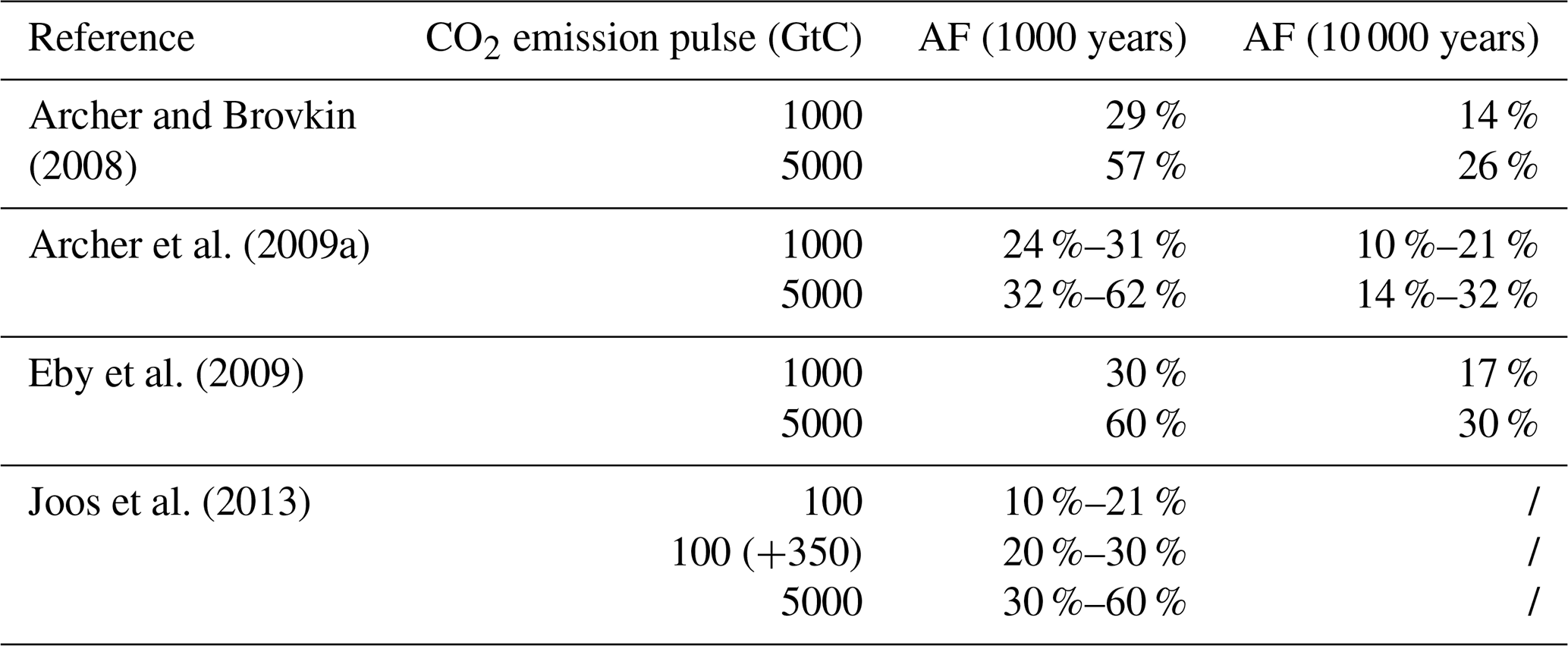
Table A2Average equilibrium airborne fractions for total emissions of around 500 to 5000 GtC according to the values given in Table A1. The equilibrium airborne fraction for 2000 GtC is extrapolated from the average equilibrium airborne fraction for the 1000 GtC and 5000 GtC scenarios. The instantaneous airborne fraction is the airborne fraction reached after 1 year (AFpeak). Airborne fractions after 1000 and 10 000 years are given. The columns highlighted in bold give the fractions of atmospheric CO2 still present 1000 and 10 000 years after the peak concentration. The numbers in the first column denote the cumulative emissions CO2 emissions with respect to pre-industrial levels.
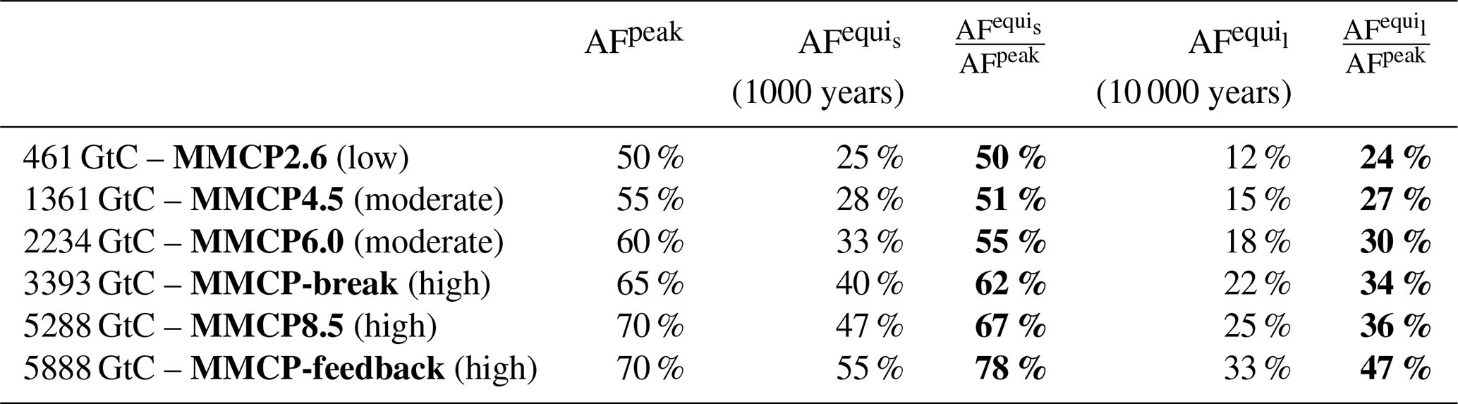
Table A3Different CO2 scenarios used in the simulations with their time of peak concentration, the values for the peak concentration, the mean concentration over the next 10 000 years, and the equivalent total emissions (calculated as in Meinshausen et al., 2011). The total cumulative emissions are an approximation for the RCP scenarios (the numbers give the total fossil fuel cumulative CO2 emissions expressed in gigatonnes of Carbon for the period 2000–2300 CE). These numbers are on top of the cumulative CO2 emissions before 2000 CE given in brackets (about 270 GtC; Ciais et al., 2013).

The LOVECLIM v1.3 model code can be downloaded from https://www.elic.ucl.ac.be/modx/index.php?id=289 (last access: 6 October 2020) (ELIC members, 2020). Model output data are available upon author request.
The supplement related to this article is available online at: https://doi.org/10.5194/esd-11-953-2020-supplement.
PH, HG, and JVB designed the experiments and JVB carried them out. HG and PH developed the model code. JVB prepared the paper with contributions from all co-authors.
The authors declare that they have no conflict of interest.
We would like to thank two anonymous reviewers and Paolo Scussolini for their detailed comments and useful feedback.
Pierre Regnier and Pierre Friedlingstein are acknowledged for their discussions on the applied impulse response function and the use of the constructed carbon dioxide scenarios. We acknowledge support through the Belgian Federal Science Policy Office within its Research Programme on Science for a Sustainable Development under contract SD/CS/06A (iCLIPS) and the Belgian National Agency for Radioactive Waste and enriched Fissile Material (ONDRAF/NIRAS).
This research has been supported by the Belgian Federal Science Policy Office (grant no. SD/CS/06A).
This paper was edited by Zhenghui Xie and reviewed by Paolo Scussolini and two anonymous referees.
Alley, R. B. and Whillans, I. M.: Response of the East Antarctica ice sheet to sea-level rise, J. Geophys. Res., 89, 6487–6493, https://doi.org/10.1029/JC089iC04p06487, 1984.
Alley, R. B., Clark, P. U., Huybrechts, P., and Joughin, I.: Ice-Sheet and Sea-Level Changes, Science, 310, 456–460, https://doi.org/10.1126/science.1114613, 2005.
Applegate, P. J., Parizek, B. R., Nicholas, R. E., Alley, R. B., and Keller, K.: Increasing temperature forcing reduces the Greenland Ice Sheet's response time scale, Clim. Dynam., 45, 2001–2011, https://doi.org/10.1007/s00382-014-2451-7, 2015.
Archer, D. and Brovkin, V.: The millennial atmospheric lifetime of anthropogenic CO2, Climatic Change, 90, 283–297, https://doi.org/10.1007/s10584-008-9413-1, 2008.
Archer, D., Eby, M., Brovkin, V., Ridgwell, A., Cao, L., Mikolajewicz, U., Caldeira, K., Matsumoto, K., Munhoven, G., Montenegro, A., and Tokos, K.: Atmospheric Lifetime of Fossil Fuel Carbon Dioxide, Annu. Rev. Earth Planet. Sci., 37, 117–134, https://doi.org/10.1146/annurev.earth.031208.100206, 2009a.
Archer, D., Buffett, B., and Brovkin, V.: Ocean methane hydrates as a slow tipping point in the global carbon cycle, P. Natl. Acad. Sci. USA., 106, 20596–20601, https://doi.org/10.1073/pnas.0800885105, 2009b.
Aschwanden, A., Fahnestock, M. A., Truffer, M., Brinkerhoff, D. J., Hock, R., Khroulev, C., Mottram, R., and Khan, S. A.: Contribution of the Greenland Ice sheet to sea level over the next millennium, Sci. Adv., 5, eaav9396, https://doi.org/10.1126/sciadv.aav9396, 2019.
Barthel, A., Agosta, C., Little, C. M., Hattermann, T., Jourdain, N. C., Goelzer, H., Nowicki, S., Seroussi, H., Straneo, F., and Bracegirdle, T. J.: CMIP5 model selection for ISMIP6 ice sheet model forcing: Greenland and Antarctica, The Cryosphere, 14, 855–879, https://doi.org/10.5194/tc-14-855-2020, 2020.
Bulthuis, K., Arnst, M., Sun, S., and Pattyn, F.: Uncertainty quantification of the multi-centennial response of the Antarctic ice sheet to climate change, The Cryosphere, 13, 1349–1380, https://doi.org/10.5194/tc-13-1349-2019, 2019.
Calov, R., Beyer, S., Greve, R., Beckmann, J., Willeit, M., Kleiner, T., Rückamp, M., Humbert, A., and Ganopolski, A.: Simulation of the future sea level contribution of Greenland with a new glacial system model, The Cryosphere, 12, 3097–3121, https://doi.org/10.5194/tc-12-3097-2018, 2018.
Chan, W.-L. and Abe-Ouchi, A.: Pliocene Model Intercomparison Project (PlioMIP2) simulations using the Model for Interdisciplinary Research on Climate (MIROC4m), Clim. Past, 16, 1523–1545, https://doi.org/10.5194/cp-16-1523-2020, 2020.
Chandan, D. and Peltier, W. R.: Regional and global climate for the mid-Pliocene using the University of Toronto version of CCSM4 and PlioMIP2 boundary conditions, Clim. Past, 13, 919–942, https://doi.org/10.5194/cp-13-919-2017, 2017.
Charbit, S., Paillard, D., and Ramstein, G.: Amount of CO2 emissions irreversibly leading to the total melting of Greenland, Geophys. Res. Lett., 35, 1–5, https://doi.org/10.1029/2008GL033472, 2008.
Church, J. A. and White, N. J.: Sea-Level Rise from the Late 19th to the Early 21st Century, Surv. Geophys., 32, 585–602, https://doi.org/10.1007/s10712-011-9119-1, 2011.
Ciais, P., Sabine, C., Bala, G., Bopp, L., Brovkin, V., Canadell, J., Chhabra, A., DeFries, R., Galloway, J., Heimann, M., Jones, C., Quéré, C. Le, Myneni, R. B., Piao, S., and Thornton, P.: Carbon and Other Biogeochemical Cycles, in: Climate Change 2013: The Physical Science Basis. Contribution of working group I to the Fifth Assessment Report of the Intergovernmental Panel on Climate Change, edited by: Stocker, T. F., Qin, D., Plattner, G.-K., Tignor, M., Allen, S. K., Boschung, J., Nauels, A., Xia, Y., Bex, V., and Midgley, P. M., Cambridge University Press, Cambridge, United Kingdom and New York, NY, USA, 2013.
Clark, P. U., Shakun, J. D., Marcott, S. A., Mix, A. C., Eby, M., Kulp, S., Levermann, A., Milne, G. A., Pfister, P. L., Santer, B. D., Schrag, D. P., Solomon, S., Stocker, T. F., Strauss, B. H., Weaver, A. J., Winkelmann, R., Archer, D., Bard, E., Goldner, A., Lambeck, K., Pierrehumbert, R. T., and Plattner, G. K.: Consequences of twenty-first-century policy for multi-millennial climate and sea-level change, Nat. Clim. Chang., 6, 360–369, https://doi.org/10.1038/nclimate2923, 2016.
Cronin, T. M.: Rapid sea-level rise, Quaternary Sci. Rev., 56, 11–30, https://doi.org/10.1016/j.quascirev.2012.08.021, 2012.
Dean, J. F., Middelburg, J. J., Röckmann, T., Aerts, R., Blauw, L. G., Egger, M., Jetten, M. S. M., de Jong, A. E. E., Meisel, O. H., Rasigraf, O., Slomp, C. P., in't Zandt M. H., and Dolman, A. J.: Methane Feedbacks to the Global Climate System in a Warmer World, Rev. Geophys., 56, 207–250, https://doi.org/10.1002/2017RG000559, 2018.
DeConto, R. M. and Pollard, D.: Contribution of Antarctica to past and future sea-level rise, Nature, 531, 591–597, https://doi.org/10.1038/nature17145, 2016.
Dickens, G. R.: Down the Rabbit Hole: toward appropriate discussion of methane release from gas hydrate systems during the Paleocene-Eocene thermal maximum and other past hyperthermal events, Clim. Past, 7, 831–846, https://doi.org/10.5194/cp-7-831-2011, 2011.
Driesschaert, E., Fichefet, T., Goosse, H., Huybrechts, P., Janssens, I., Mouchet, A., Munhoven, G., Brovkin, V., and Weber, S. L.: Modeling the influence of Greenland ice sheet melting on the Atlantic meridional overturning circulation during the next millennia, Geophys. Res. Lett., 34, 1–5, https://doi.org/10.1029/2007GL029516, 2007.
Eby, M., Zickfeld, K., Montenegro, A., Archer, D., Meissner, K. J., and Weaver, A. J.: Lifetime of Anthropogenic Climate Change: Millennial Time Scales of Potential CO2 and Surface Temperature Perturbations, J. Climate, 22, 2501–2511, https://doi.org/10.1175/2008JCLI2554.1, 2009.
Eby, M., Weaver, A. J., Alexander, K., Zickfeld, K., Abe-Ouchi, A., Cimatoribus, A. A., Crespin, E., Drijfhout, S. S., Edwards, N. R., Eliseev, A. V., Feulner, G., Fichefet, T., Forest, C. E., Goosse, H., Holden, P. B., Joos, F., Kawamiya, M., Kicklighter, D., Kienert, H., Matsumoto, K., Mokhov, I. I., Monier, E., Olsen, S. M., Pedersen, J. O. P., Perrette, M., Philippon-Berthier, G., Ridgwell, A., Schlosser, A., Schneider von Deimling, T., Shaffer, G., Smith, R. S., Spahni, R., Sokolov, A. P., Steinacher, M., Tachiiri, K., Tokos, K., Yoshimori, M., Zeng, N., and Zhao, F.: Historical and idealized climate model experiments: an intercomparison of Earth system models of intermediate complexity, Clim. Past, 9, 1111–1140, https://doi.org/10.5194/cp-9-1111-2013, 2013.
Edwards, T. L., Brandon, M. A., Durand, G., Edwards, N. R., Golledge, N. R., Holden, P. B., Nias, I. J., Payne, A. J., Ritz, C., and Wernecke, A.: Revisiting Antarctic ice loss due to marine ice-cliff instability, Nature, 566, 58–64, https://doi.org/10.1038/s41586-019-0901-4, 2019.
ELIC members: LOVECLIM version 1.3, available at: https://www.elic.ucl.ac.be/modx/index.php?id=289, last access: 6 October 2020.
Farinotti, D., Huss, M., Fürst, J. J., Landmann, J., Machguth, H., Maussion, F., and Pandit, A.: A consensus estimate for the ice thickness distribution of all glaciers on Earth, Nat. Geosci., 12, 168–173, https://doi.org/10.1038/s41561-019-0300-3, 2019.
Feistel, R.: Extended equation of state for seawater at elevated temperature and salinity, Desalination, 250, 14–18, https://doi.org/10.1016/j.desal.2009.03.020, 2010.
Fettweis, X., Franco, B., Tedesco, M., van Angelen, J. H., Lenaerts, J. T. M., van den Broeke, M. R., and Gallée, H.: Estimating the Greenland ice sheet surface mass balance contribution to future sea level rise using the regional atmospheric climate model MAR, The Cryosphere, 7, 469–489, https://doi.org/10.5194/tc-7-469-2013, 2013.
Foster, G. L. and Rohling, E. J.: Relationship between sea level and climate forcing by CO2 on geological timescales, P. Natl. Acad. Sci. USA, 110, 1209–1214, https://doi.org/10.1073/pnas.1216073110, 2013.
Fretwell, P., Pritchard, H. D., Vaughan, D. G., Bamber, J. L., Barrand, N. E., Bell, R., Bianchi, C., Bingham, R. G., Blankenship, D. D., Casassa, G., Catania, G., Callens, D., Conway, H., Cook, A. J., Corr, H. F. J., Damaske, D., Damm, V., Ferraccioli, F., Forsberg, R., Fujita, S., Gim, Y., Gogineni, P., Griggs, J. A., Hindmarsh, R. C. A., Holmlund, P., Holt, J. W., Jacobel, R. W., Jenkins, A., Jokat, W., Jordan, T., King, E. C., Kohler, J., Krabill, W., Riger-Kusk, M., Langley, K. A., Leitchenkov, G., Leuschen, C., Luyendyk, B. P., Matsuoka, K., Mouginot, J., Nitsche, F. O., Nogi, Y., Nost, O. A., Popov, S. V., Rignot, E., Rippin, D. M., Rivera, A., Roberts, J., Ross, N., Siegert, M. J., Smith, A. M., Steinhage, D., Studinger, M., Sun, B., Tinto, B. K., Welch, B. C., Wilson, D., Young, D. A., Xiangbin, C., and Zirizzotti, A.: Bedmap2: improved ice bed, surface and thickness datasets for Antarctica, The Cryosphere, 7, 375–393, https://doi.org/10.5194/tc-7-375-2013, 2013.
Frigola, A., Prange, M., and Schulz, M.: Boundary conditions for the Middle Miocene Climate Transition (MMCT v1.0), Geosci. Model Dev., 11, 1607–1626, https://doi.org/10.5194/gmd-11-1607-2018, 2018.
Frölicher, T. L. and Paynter, D. J.: Extending the relationship between global warming and cumulative carbon emissions to multi-millennial timescales, Environ. Res. Lett., 10, 075002, https://doi.org/10.1088/1748-9326/10/7/075002, 2015.
Ganopolski A. and Rahmstorf S.: Rapid changes of glacial climate simulated in a coupled climate model, Nature, 409, 153–158, https://doi.org/10.1038/35051500, 2001.
Gasson, E., DeConto, R. M., Pollard, D., and Levy, R. H.: Dynamic Antarctic ice sheet during the early to mid-Miocene, P. Natl. Acad. Sci. USA, 113, 3459–3464, https://doi.org/10.1073/pnas.1516130113, 2016.
Gillett, N. P., Arora, V. K., Zickfeld, K., Marshall, S. J., and Merryfield, W. J.: Ongoing climate change following a complete cessation of carbon dioxide emissions, Nat. Geosci., 4, 83–87, https://doi.org/10.1038/ngeo1047, 2011.
Goelzer, H., Huybrechts, P., Raper, S. C. B., Loutre, M. F., Goosse, H., and Fichefet, T.: Millennial total sea-level commitments projected with the Earth system model of intermediate complexity LOVECLIM, Environ. Res. Lett., 7, 045401, https://doi.org/10.1088/1748-9326/7/4/045401, 2012.
Goelzer, H., Huybrechts, P., Loutre, M.-F., and Fichefet, T.: Impact of ice sheet meltwater fluxes on the climate evolution at the onset of the Last Interglacial, Clim. Past, 12, 1721–1737, https://doi.org/10.5194/cp-12-1721-2016, 2016a.
Goelzer, H., Huybrechts, P., Loutre, M.-F., and Fichefet, T.: Last Interglacial climate and sea-level evolution from a coupled ice sheet-climate model, Clim. Past, 12, 2195–2213, https://doi.org/10.5194/cp-12-2195-2016, 2016b.
Goelzer, H., Coulon, V., Pattyn, F., de Boer, B., and van de Wal, R.: Brief communication: On calculating the sea-level contribution in marine ice-sheet models, The Cryosphere, 14, 833–840, https://doi.org/10.5194/tc-14-833-2020, 2020a.
Goelzer, H., Nowicki, S., Payne, A., Larour, E., Seroussi, H., Lipscomb, W. H., Gregory, J., Abe-Ouchi, A., Shepherd, A., Simon, E., Agosta, C., Alexander, P., Aschwanden, A., Barthel, A., Calov, R., Chambers, C., Choi, Y., Cuzzone, J., Dumas, C., Edwards, T., Felikson, D., Fettweis, X., Golledge, N. R., Greve, R., Humbert, A., Huybrechts, P., Le clec'h, S., Lee, V., Leguy, G., Little, C., Lowry, D. P., Morlighem, M., Nias, I., Quiquet, A., Rückamp, M., Schlegel, N.-J., Slater, D., Smith, R., Straneo, F., Tarasov, L., van de Wal, R., and van den Broeke, M.: The future sea-level contribution of the Greenland ice sheet: a multi-model ensemble study of ISMIP6, The Cryosphere Discuss., https://doi.org/10.5194/tc-2019-319, in review, 2020b.
Golledge, N. R.: Long-term projections of sea-level rise from ice sheets, Wiley Interdiscip. Rev. Clim. Change, 11, e634, https://doi.org/10.1002/wcc.634, 2020.
Golledge, N. R., Menviel, L., Carter, L., Fogwill, C. J., England, M. H., Cortese, G., and Levy, R. H.: Antarctic contribution to meltwater pulse 1A from reduced Southern Ocean overturning, Nat. Commun., 5, 5107, https://doi.org/10.1038/ncomms6107, 2014.
Golledge, N. R., Kowalewski, D. E., Naish, T. R., Levy, R. H., Fogwill, C. J., and Gasson, E. G. W.: The multi-millennial Antarctic commitment to future sea-level rise, Nature, 526, 421–425, https://doi.org/10.1038/nature15706, 2015.
Goosse, H. and Fichefet, T.: Importance of ice-ocean interactions for the global ocean circulation: A model study, J. Geophys. Res.-Oceans, 104, 23337–23355, https://doi.org/10.1029/1999jc900215, 1999.
Goosse, H., Brovkin, V., Fichefet, T., Haarsma, R., Huybrechts, P., Jongma, J., Mouchet, A., Selten, F., Barriat, P.-Y., Campin, J.-M., Deleersnijder, E., Driesschaert, E., Goelzer, H., Janssens, I., Loutre, M.-F., Morales Maqueda, M. A., Opsteegh, T., Mathieu, P.-P., Munhoven, G., Pettersson, E. J., Renssen, H., Roche, D. M., Schaeffer, M., Tartinville, B., Timmermann, A., and Weber, S. L.: Description of the Earth system model of intermediate complexity LOVECLIM version 1.2, Geosci. Model Dev., 3, 603–633, https://doi.org/10.5194/gmd-3-603-2010, 2010.
Griffis, T. J., Chen, Z., Baker, J. M., Wood, J. D., Millet, D. B., Lee, X., Venterea, R. T., and Turner, P. A.: Nitrous oxide emissions are enhanced in a warmer and wetter world, P. Natl. Acad. Sci. USA, 114, 12081–12085, https://doi.org/10.1073/pnas.1704552114, 2017.
Hasselmann, K., Latif, M., Hooss, G., Azar, C., Edenhofer, O., Jaeger, C. C., Johannessen, O. M., Kemfert, C., Welp, M., and Wokaun, A.: The Challenge of Long-Term Climate Change, Science, 302, 1923–1925, https://doi.org/10.1126/science.1090858, 2003.
Hay, C. C., Morrow, E., Kopp, R. E., and Mitrovica, J. X.: Probabilistic reanalysis of twentieth-century sea-level rise, Nature, 517, 481–484, https://doi.org/10.1038/nature14093, 2015.
Hieronymus, M.: An update on the thermosteric sea level rise commitment to global warming, Environ. Res. Lett., 14, 054018, https://doi.org/10.1088/1748-9326/ab1c31, 2019.
Hock, R., Bliss, A., Marzeion, B., Giesen, R. H., Hirabayashi, Y., Huss, M., Radic, V., and Slangen, A. B. A.: GlacierMIP – A model intercomparison of global-scale glacier mass balance models and projections, J. Glaciol., 65, 453–467, https://doi.org/10.1017/jog.2019.22, 2019.
Huss, M. and Hock, R.: A new model for global glacier change and sea-level rise, Front. Earth Sci., 3, 54, https://doi.org/10.3389/feart.2015.00054, 2015.
Huybrechts, P.: Glaciological Modelling of the Late Cenozoic East Antarctic Ice Sheet: Stability or Dynamism?, Geogr. Ann. Ser. A, Phys. Geogr., 75, 221–238, https://doi.org/10.1080/04353676.1993.11880395, 1993.
Huybrechts, P. and de Wolde, J.: The Dynamic Response of the Greenland and Antarctic Ice Sheets to Multiple-Century Climatic Warming, J. Climate, 12, 2169–2188, https://doi.org/10.1175/1520-0442(1999)012<2169:tdrotg>2.0.co;2, 1999.
Huybrechts, P., Goelzer, H., Janssens, I., Driesschaert, E., Fichefet, T., Goosse, H., and Loutre, M. F.: Response of the Greenland and Antarctic Ice Sheets to Multi-Millennial Greenhouse Warming in the Earth System Model of Intermediate Complexity LOVECLIM, Surv. Geophys., 32, 397–416, https://doi.org/10.1007/s10712-011-9131-5, 2011.
Jackson, L. P. and Jevrejeva, S.: A probabilistic approach to 21st century regional sea-level projections using RCP and High-end scenarios, Global Planet. Change, 146, 179–189, https://doi.org/10.1016/j.gloplacha.2016.10.006, 2016.
Jansen, M. F., Nadeau, L.-P., and Merlis, T. M.: Transient versus Equilibrium Response of the Ocean's Overturning Circulation to Warming, J. Climate, 31, 5147–5163, https://doi.org/10.1175/JCLI-D-17-0797.1, 2018.
Joos, F., Roth, R., Fuglestvedt, J. S., Peters, G. P., Enting, I. G., von Bloh, W., Brovkin, V., Burke, E. J., Eby, M., Edwards, N. R., Friedrich, T., Frölicher, T. L., Halloran, P. R., Holden, P. B., Jones, C., Kleinen, T., Mackenzie, F. T., Matsumoto, K., Meinshausen, M., Plattner, G.-K., Reisinger, A., Segschneider, J., Shaffer, G., Steinacher, M., Strassmann, K., Tanaka, K., Timmermann, A., and Weaver, A. J.: Carbon dioxide and climate impulse response functions for the computation of greenhouse gas metrics: a multi-model analysis, Atmos. Chem. Phys., 13, 2793–2825, https://doi.org/10.5194/acp-13-2793-2013, 2013.
Jungclaus, J. H., Bard, E., Baroni, M., Braconnot, P., Cao, J., Chini, L. P., Egorova, T., Evans, M., González-Rouco, J. F., Goosse, H., Hurtt, G. C., Joos, F., Kaplan, J. O., Khodri, M., Klein Goldewijk, K., Krivova, N., LeGrande, A. N., Lorenz, S. J., Luterbacher, J., Man, W., Maycock, A. C., Meinshausen, M., Moberg, A., Muscheler, R., Nehrbass-Ahles, C., Otto-Bliesner, B. I., Phipps, S. J., Pongratz, J., Rozanov, E., Schmidt, G. A., Schmidt, H., Schmutz, W., Schurer, A., Shapiro, A. I., Sigl, M., Smerdon, J. E., Solanki, S. K., Timmreck, C., Toohey, M., Usoskin, I. G., Wagner, S., Wu, C.-J., Yeo, K. L., Zanchettin, D., Zhang, Q., and Zorita, E.: The PMIP4 contribution to CMIP6 – Part 3: The last millennium, scientific objective, and experimental design for the PMIP4 past1000 simulations, Geosci. Model Dev., 10, 4005–4033, https://doi.org/10.5194/gmd-10-4005-2017, 2017.
Kalnay, E., Kanamitsu, M., Kistler, R., Collins, W., Deaven, D., Gandin, L., Iredell, M., Saha, S., White, G., Woollen, J., Zhu, Y., Chelliah, M., Ebisuzaki, W., Higgins, W., Janowiak, J., Mo, K. C., Ropelewski, C., Wang, J., Leetmaa, A., Reynolds, R., Jenne, R., and Joseph, D.: The NCEP/NCAR 40-year reanalysis project, B. Am. Meteorol. Soc., 77, 437–471, https://doi.org/10.1175/1520-0477(1996)077<0437:TNYRP>2.0.CO;2, 1996.
Kirschke, S., Bousquet, P., Ciais, P., Saunois, M., Canadell, J. G., Dlugokencky, E. J., Bergamaschi, P., Bergmann, D., Blake, D. R., Bruhwiler, L., Cameron-Smith, P., Castaldi, S., Chevallier, F., Feng, L., Fraser, A., Heimann, M., Hodson, E. L., Houweling, S., Josse, B., Fraser, P. J., Krummel, P. B., Lamarque, J. F., Langenfelds, R. L., Le Quéré, C., Naik, V., O'doherty, S., Palmer, P. I., Pison, I., Plummer, D., Poulter, B., Prinn, R. G., Rigby, M., Ringeval, B., Santini, M., Schmidt, M., Shindell, D. T., Simpson, I. J., Spahni, R., Steele, L. P., Strode, S. A., Sudo, K., Szopa, S., Van Der Werf, G. R., Voulgarakis, A., Van Weele, M., Weiss, R. F., Williams, J. E., and Zeng, G.: Three decades of global methane sources and sinks, Nat. Geosci., 6, 813–823, https://doi.org/10.1038/ngeo1955, 2013.
Kopp, R. E., DeConto, R. M., Bader, D. A., Hay, C. C., Horton, R. M., Kulp, S., Oppenheimer, M., Pollard, D., and Strauss, B. H.: Evolving Understanding of Antarctic Ice-Sheet Physics and Ambiguity in Probabilistic Sea-Level Projections, Earth's Futur., 5, 1217–1233, https://doi.org/10.1002/2017EF000663, 2017.
Levermann, A., Clark, P. U., Marzeion, B., Milne, G. A., Pollard, D., Radic, V., and Robinson, A.: The multimillennial sea-level commitment of global warming, P. Natl. Acad. Sci. USA, 110, 13745–13750, https://doi.org/10.1073/pnas.1219414110, 2013.
Levermann, A., Winkelmann, R., Albrecht, T., Goelzer, H., Golledge, N. R., Greve, R., Huybrechts, P., Jordan, J., Leguy, G., Martin, D., Morlighem, M., Pattyn, F., Pollard, D., Quiquet, A., Rodehacke, C., Seroussi, H., Sutter, J., Zhang, T., Van Breedam, J., Calov, R., DeConto, R., Dumas, C., Garbe, J., Gudmundsson, G. H., Hoffman, M. J., Humbert, A., Kleiner, T., Lipscomb, W. H., Meinshausen, M., Ng, E., Nowicki, S. M. J., Perego, M., Price, S. F., Saito, F., Schlegel, N.-J., Sun, S., and van de Wal, R. S. W.: Projecting Antarctica's contribution to future sea level rise from basal ice shelf melt using linear response functions of 16 ice sheet models (LARMIP-2), Earth Syst. Dynam., 11, 35–76, https://doi.org/10.5194/esd-11-35-2020, 2020.
Liu, W., Liu, Z., and Brady, E. C.: Why is the AMOC Monostable in Coupled General Circulation Models?, J. Climate, 27, 2427–2443, https://doi.org/10.1175/JCLI-D-13-00264.1, 2014.
Lord, N. S., Ridgwell, A., Thorne, M. C., and Lunt, D. J.: An impulse response function for the “long tail” of excess atmospheric CO2 in an Earth system model, Global Biogeochem. Cy., 30, 2–17, https://doi.org/10.1002/2014GB005074, 2016.
Loutre, M. F., Mouchet, A., Fichefet, T., Goosse, H., Goelzer, H., and Huybrechts, P.: Evaluating climate model performance with various parameter sets using observations over the recent past, Clim. Past, 7, 511–526, https://doi.org/10.5194/cp-7-511-2011, 2011.
Loutre, M. F., Fichefet, T., Goosse, H., Huybrechts, P., Goelzer, H., and Capron, E.: Factors controlling the last interglacial climate as simulated by LOVECLIM1.3, Clim. Past, 10, 1541–1565, https://doi.org/10.5194/cp-10-1541-2014, 2014.
Maier-Reimer, E. and Hasselmann, K.: Transport and storage of CO2 in the ocean – an inorganic ocean-circulation carbon cycle model, Clim. Dynam., 2, 63–90, https://doi.org/10.1007/BF01054491, 1987.
Marzeion, B., Hock, R., Anderson, B., Bliss, A., Champollion, N., Fujita, K., Matthias, H., Immerzeel, W. W., Kraaijenbrink, P., Malles, J.-H., Maussion, F., Radic ì, V., Rounce, D. R., Sakai, A., Shannon, S., van de Wal, R., and Zekollari, H.: Partitioning the uncertainty of ensemble projections of global glacier mass change, Earth's Future, 8, e2019EF001470, https://doi.org/10.1029/2019EF001470, 2020.
Matthews, H. D., Zickfeld, K., Knutti, R., and Allen, M. R.: Focus on cumulative emissions, global carbon budgets and the implications for climate mitigation targets, Environ. Res. Lett., 13, 010201, https://doi.org/10.1088/1748-9326/aa98c9, 2018.
McGlade, C. and Ekins, P.: The geographical distribution of fossil fuels unused when limiting global warming to 2 ∘C, Nature, 517, 187–190, https://doi.org/10.1038/nature14016, 2015.
Mecking, J. V., Drijfhout, S. S. Jackson, L. C., and Andrews, M. B.: The effect of model bias on Atlantic freshwater transport and implications for AMOC bi-stability, Tellus A, 69, 1299910, https://doi.org/10.1038/35051500, 2017.
Meinshausen, M., Smith, S. J., Calvin, K., Daniel, J. S., Kainuma, M. L. T., Lamarque, J-F., Matsumoto, K., Montzka, S. A., Raper, S. C. B., Riahi, K., Thomson, A., Velders, G. J. M., and van Vuuren, D. P. P.: The RCP greenhouse gas concentrations and their extensions from 1765 to 2300, Climatic Change, 109, 213–241, https://doi.org/10.1007/s10584-011-0156-z, 2011.
Mengel, M., Levermann, A., Frieler, K., Robinson, A., Marzeion, B., and Winkelmann, R.: Future sea level rise constrained by observations and long-term commitment, P. Natl. Acad. Sci. USA, 113, 2597–2602, https://doi.org/10.1073/pnas.1500515113, 2016.
Miller, K. G., Kominz, M. A., Browning, J. V., Wright, J. D., Mountain, G. S., Katz, M. E., Sugarman, P. J., Cramer, B. S., Christie-Blick, N., and Pekar, S. F.: The Phanerozoic Record of Global Sea-Level Change, Science, 310, 1293–1298, https://doi.org/10.1126/science.1116412, 2005.
Oppenheimer, M., Glavovic, B., Hinkel, J., van de Wal, R. S. W., Magnan, A., Abd-Elgawad, A., Cai, R., Cifuentes Jara, M., DeConto, R., Ghosh, T., Hay, J., Isla, F., Marzeion, B., Meyssignac, B., and Sebesvari, Z.: Sea Level Rise and Implications for Low Lying Islands, Coasts and Communities, in: IPCC Special Report on the Ocean and Cryosphere in a Changing Climate, edited by: Pörtner, H.-O., Roberts, D. C., Masson-Delmotte, V., Zhai, P., Tignor, M., Poloczanska, E., Mintenbeck, K., Nicolai, M., Okem, A., Petzold, J., Rama, B., and Weyer, N., p. 169, in press, 2019.
Opsteegh, J. D., Haarsma, R. J., Selten, F. M., and Kattenberg, A.: ECBILT: A dynamic alternative to mixed boundary conditions in ocean models, Tellus A, 50, 348–367, https://doi.org/10.3402/tellusa.v50i3.14524, 1998.
Paxman, J. G., Jamieson S. S. R., Hochmuth, K., Gohl, K., Bentley, M. J., Leitchenkov, G., and Ferracioli, F.: Reconstructions of the Antarctic topography since the Eocene-Oligocene boundary, Palaeogeogr. Palaeocl., 535, 109346, https://doi.org/10.1016/j.palaeo.2019.109346, 2019.
Piñero, E., Marquardt, M., Hensen, C., Haeckel, M., and Wallmann, K.: Estimation of the global inventory of methane hydrates in marine sediments using transfer functions, Biogeosciences, 10, 959–975, https://doi.org/10.5194/bg-10-959-2013, 2013
Pollard, D. and DeConto, R. M.: Hysteresis in Cenozoic Antarctic ice-sheet variations, Global Planet. Change, 45, 9–21, https://doi.org/10.1016/j.gloplacha.2004.09.011, 2005.
Pollard, D., DeConto, R. M., and Alley, R. B.: Potential Antarctic Ice Sheet retreat driven by hydrofracturing and ice cliff failure, Earth Planet. Sci. Lett., 412, 112–121, https://doi.org/10.1016/j.epsl.2014.12.035, 2015.
Pörtner, H.-O., Roberts, D. C., Masson-Delmotte, V., Zhai, P., Tignor, M., Poloczanska, E., Mintenbeck, K., Nicolai, M., Okem, A., Petzold, J., Rama, B., and Weyer, N. W. (Eds.): IPCC Special Report on the Ocean and Cryosphere in a Changing Climate (SROCC), Cambridge University Press, in press, 2019.
Rahmstorf, S., Crucifix, M., Ganopolski, A., Goosse, H., Kamenkovich, I., Knutti, R., Lohmann, G., Marsh, R., Mysak, L. A., Wang, Z., and Weaver, A. J.: Thermohaline circulation hysteresis: A model intercomparison, Geophys. Res. Lett., 32, L23605, https://doi.org/10.1029/2005GL023655, 2005.
Raper, S. C. B. and Braithwaite, R. J.: Low sea level rise projections from mountain glaciers and icecaps under global warming, Nature, 439, 311–313, https://doi.org/10.1038/nature04448, 2006.
Robinson, A., Calov, R., and Ganopolski, A.: Multistability and critical thresholds of the Greenland ice sheet, Nat. Clim. Chang., 2, 429–432, https://doi.org/10.1038/nclimate1449, 2012.
Rogelj, J., Schaeffer, M., Friedlingstein, P., Gillett, N. P., van Vuuren, D. P., Riahi, K., Allen, M., and Knutti, R.: Differences between carbon budget estimates unravelled, Nat. Clim. Chang., 6, 245–252, https://doi.org/10.1038/nclimate2868, 2016.
Ruppel, C. D. and Kessler, J. D.: The interaction of climate change and methane hydrates, Rev. Geophys., 55, 126–168, https://doi.org/10.1002/2016RG000534, 2017.
Schuur, E. A. G., McGuire, A. D., Schädel, C., Grosse, G., Harden, J. W., Hayes, D. J., Hugelius, G., Koven, C. D., Kuhry, P., Lawrence, D. M., Natali, S. M., Olefeldt, D., Romanovsky, V. E., Schaefer, K., Turetsky, M. R., Treat, C. C., and Vonk, J. E.: Climate change and the permafrost feedback, Nature, 520, 171–179, https://doi.org/10.1038/nature14338, 2015.
Seroussi, H., Nowicki, S., Payne, A. J., Goelzer, H., Lipscomb, W. H., Abe Ouchi, A., Agosta, C., Albrecht, T., Asay-Davis, X., Barthel, A., Calov, R., Cullather, R., Dumas, C., Gladstone, R., Golledge, N., Gregory, J. M., Greve, R., Hatterman, T., Hoffman, M. J., Humbert, A., Huybrechts, P., Jourdain, N. C., Kleiner, T., Larour, E., Leguy, G. R., Lowry, D. P., Little, C. M., Morlighem, M., Pattyn, F., Pelle, T., Price, S. F., Quiquet, A., Reese, R., Schlegel, N.-J., Shepherd, A., Simon, E., Smith, R. S., Straneo, F., Sun, S., Trusel, L. D., Van Breedam, J., van de Wal, R. S. W., Winkelmann, R., Zhao, C., Zhang, T., and Zwinger, T.: ISMIP6 Antarctica: a multi-model ensemble of the Antarctic ice sheet evolution over the 21st century, The Cryosphere Discuss., https://doi.org/10.5194/tc-2019-324, in review, 2020.
Solomon, S., Plattner, G. K., Knutti, R., and Friedlingstein, P.: Irreversible climate change due to carbon dioxide emissions, P. Natl. Acad. Sci. USA, 106, 1704–1709, https://doi.org/10.1073/pnas.0812721106, 2009.
Stocker, T. F.: The Seesaw Effect, Science, 282, 61–62, https://doi.org/10.1126/science.282.5386.61, 1998.
Swingedouw, D., Fichefet, T., Huybrechts, P., Goosse, H., Driesschaert, E. and Loutre, M. F.: Antarctic ice-sheet melting provides negative feedbacks on future climate warming, Geophys. Res. Lett., 35, 2–5, https://doi.org/10.1029/2008GL034410, 2008.
Swingedouw, D., Fichefet, T., Goosse, H., and Loutre, M. F.: Impact of transient freshwater releases in the Southern Ocean on the AMOC and climate, Clim. Dynam., 33, 365–381, https://doi.org/10.1007/s00382-008-0496-1, 2009.
Treude, T., Boetius, A., Knittel, K., Wallmann, K., and Jørgensen, B. B.: Anaerobic oxidation of methane above gas hydrates at Hydrate Ridge, NE Pacific Ocean, Mar. Ecol.-Prog. Ser., 264, 1–14, https://doi.org/10.3354/meps264001, 2003.
Vizcaíno, M., Mikolajewicz, U., Gröger, M., Maier-Reimer, E., Schurgers, G., and Winguth, A. M. E.: Long-term ice sheet-climate interactions under anthropogenic greenhouse forcing simulated with a complex Earth System Model, Clim. Dynam., 31, 665–690, https://doi.org/10.1007/s00382-008-0369-7, 2008.
Watson, C. S., White, N. J., Church, J. A., King, M. A., Burgette, R. J., and Legresy, B.: Unabated global mean sea-level rise over the satellite altimeter era, Nat. Clim. Chang., 5, 565–568, https://doi.org/10.1038/nclimate2635, 2015.
Winkelmann, R., Levermann, A., Martin, M. A., and Frieler, K.: Increased future ice discharge from Antarctica owing to higher snowfall, Nature, 492, 239–242, https://doi.org/10.1038/nature11616, 2012.
Winkelmann, R., Levermann, A., Ridgwell, A., and Caldeira, K.: Combustion of available fossil fuel resources sufficient to eliminate the Antarctic Ice Sheet, Sci. Adv., 1, 1–6, https://doi.org/10.1126/sciadv.1500589, 2015.
Zeebe, R. E. and Lourens, L. J.: Solar System chaos and the Paleocene-Eocene boundary age constrained by geology and astronomy, Science, 365, 926–929, https://doi.org/10.1126/science.aax0612, 2019.
Zeebe, R. E. and Zachos, J. C.: Long-term legacy of massive carbon input to the Earth system: Anthropocene versus Eocene, Philos. T. R. Soc. A, 371, 20120006, https://doi.org/10.1098/rsta.2012.0006, 2013.
Zickfeld, K., Arora, V. K., and Gillett, N. P.: Is the climate response to CO2 emissions path dependent?, Geophys. Res. Lett., 39, 1–6, https://doi.org/10.1029/2011GL050205, 2012.
Zickfeld, K., Eby, M., Weaver, A. J., Alexander, K., Crespin, E.,Edwards, N. R., Eliseev, A. V., Feulner, G., Fichefet, T., Forest, C. E., Friedlingstein, P., Goosse, H., Holden, P. B., Joos, F., Kawamiya, M., Kicklighter, D., Kienert, H., Matsumoto, K., Mokhov, I. I., Monier, E., Olsen, S. M., Pedersen, J. O. P., Perrette, M., Philippon-Berthier, G. G., Ridgwell, A., Schlosser, A., Schneider Von Deimling, T., Shaffer, G., Sokolov, A., Spahni, R., Steinacher, M., Tachiiri, K., Tokos, K. S., Yoshimori, M., Zeng, N., and Zhao, F.: Long-Term Climate Change Commitment and Reversibility: An EMIC Intercomparison, J. Climate, 26, 5782–5809, https://doi.org/10.1175/jcli-d-12-00584.1, 2013.
- Abstract
- Introduction
- Model description and initialization
- Scenario description
- Climate response and global sea-level budget of individual terms
- Global mean sea-level change
- Global mean sea-level change uncertainty
- Long-term sea-level rise in the light of the geological record
- Discussion
- Conclusions
- Appendix A: Construction of the carbon dioxide concentration scenarios
- Code and data availability
- Author contributions
- Competing interests
- Acknowledgements
- Financial support
- Review statement
- References
- Supplement