the Creative Commons Attribution 4.0 License.
the Creative Commons Attribution 4.0 License.
 | 03 Nov 2020
Effect of changing ocean circulation on deep ocean temperature in the last millennium
Jeemijn Scheen
Thomas F. Stocker
Paleoreconstructions and modern observations provide us with anomalies of surface temperature over the past millennium. The history of deep ocean temperatures is much less well-known and was simulated in a recent study for the past 2000 years under forced surface temperature anomalies and fixed ocean circulation. In this study, we simulate the past 800 years with an illustrative forcing scenario in the Bern3D ocean model, which enables us to assess the impact of changes in ocean circulation on deep ocean temperature. We quantify the effect of changing ocean circulation by comparing transient simulations (where the ocean dynamically adjusts to anomalies in surface temperature – hence density) to simulations with fixed ocean circulation. We decompose temperature, ocean heat content and meridional heat transport into the contributions from changing ocean circulation and changing sea surface temperature (SST). In the deep ocean, the contribution from changing ocean circulation is found to be as important as the changing SST signal itself. Firstly, the small changes in ocean circulation amplify the Little Ice Age signal at around 3 km depth by at least a factor of 2, depending on the basin. Secondly, they fasten the arrival of this atmospheric signal in the Pacific and Southern Ocean at all depths, whereas they delay the arrival in the Atlantic between about 2.5 and 3.5 km by two centuries. This delay is explained by an initial competition between the Little Ice Age cooling and a warming due to an increase in relatively warmer North Atlantic Deep Water at the cost of Antarctic Bottom Water. Under the consecutive Atlantic meridional overturning circulation (AMOC) slowdown, this shift in water masses is inverted and ageing of the water causes a late additional cooling. Our results suggest that small changes in ocean circulation can have a large impact on the amplitude and timing of ocean temperature anomalies below 2 km depth.
- Article
(10947 KB) - Full-text XML
- BibTeX
- EndNote


The climate period from 1200 to 1750 CE manifests modes of natural variability and response to solar and volcanic forcing without the substantial anthropogenic radiative forcing from increased greenhouse gas concentrations (Masson-Delmotte et al., 2013). A growing paleoclimatic database of surface reconstructions exists that quantifies this natural variability with at least continental resolution (Mann et al., 1998, 2009; McGregor et al., 2015; Neukom et al., 2019; PAGES 2k Consortium, 2013; Emile-Geay et al., 2017). Early instrumental records, based on surface measurements and their combination with models, permit the separation of climate responses due to solar and volcanic forcing respectively (Brönnimann et al., 2019), but oceanic reconstructions below the sea surface are scarce for the last millennium (Moffa-Sánchez et al., 2019). Therefore, models can be of great value by simulating past and present deep ocean temperatures in agreement with paleoclimatic reconstructions at the surface.
This study focuses on the propagation of atmospheric temperature anomalies into the deep ocean and is motivated by Gebbie and Huybers (2019), who investigated this during the past 2000 years. They used an ocean model with fixed circulation, which they inferred from modern observations and constrained by measurements of the legendary HMS Challenger expedition of 1872–1876. The changes they found in deep ocean temperature in the Atlantic and Pacific are delayed responses to variations of the forced surface climate. We wonder to what extent their results would be different with a model that permits a dynamical response of the circulation to the forcing. In this study, we test this with the Bern3D model.
Previous studies have pointed out that temperature cannot always be approximated as a passive tracer, since it induces circulation changes, which influence the patterns of heat uptake (Banks and Gregory, 2006; Xie and Vallis, 2011; Winton et al., 2013; Marshall et al., 2015; Garuba and Klinger, 2016). These authors used various approaches to separate the effects of changing circulation (also called redistribution transport) and changing sea surface temperature (SST). Banks and Gregory (2006), Marshall et al. (2015) and Garuba and Klinger (2016) used a passive tracer that diagnoses the effect of changing SST only, whereas Xie and Vallis (2011) used a tracer diagnosing the effect of changing circulation only, and Winton et al. (2013) ran simulations with artificially fixed (FIX) ocean circulation in addition to transient (TRA) simulations with dynamically changing circulation. Here we follow the latter approach, although with ocean-only simulations in order to make sure that fixed and transient simulations undergo the exact same surface boundary conditions. By prescribing these SST and sea surface salinity (SSS) fields, we cannot quantify differences in global ocean heat uptake that arise from different ocean–atmosphere interactions, as was done in Winton et al. (2013). In exchange, this allows us to quantify the downward propagation of small temperature anomalies to the abyss and the spatial pattern of heat uptake without biases due to ocean–atmosphere feedbacks, which differ between transient and fixed simulations.
The paper is organized as follows. Section 2 presents the model and the methods needed to disentangle surface signal changes from those caused by circulation changes. In Sect. 3, we analyse the propagation of temperature signals into the deep ocean and decompose them according to different physical mechanisms. Section 4 investigates the causes of leads and lags registered at depth in the different ocean basins, including their sensitivity to changes in mixing and wind stress. In Sect. 5, we compare our results with the study of Gebbie and Huybers (2019), and we conclude in Sect. 6.
2.1 Model description
We use an earth system model of intermediate complexity (EMIC), the Bern3D model version 2.0, developed by Ritz et al. (2011) and systematically constrained by observations (Roth et al., 2014). The model consists of a three-dimensional dynamic ocean circulation model with 32 depth layers coupled to a one-layer atmosphere and a land biosphere. The ocean component of the model is based on frictional geostrophic balance equations (Edwards et al., 1998; Müller et al., 2006), and the atmosphere consists of an energy balance model including a parametrized hydrological cycle (Ritz et al., 2011). The Bern3D has an equilibrium climate sensitivity of 3.0 ∘C in the standard version. Seasonally varying winds are added as a fixed forcing. Sea-ice growth and melt are thermodynamically simulated. The horizontal grid resolution is 40×41 cells, and the time step is 3.8 d (Roth et al., 2014, Appendix A). Because of its relatively coarse resolution and reduced complexity in the atmosphere, the model is well suited for long simulations and sensitivity studies. For example, 5000 model years can be simulated within 24 h.
Here, we use the idealized age tracer, which provides information about changes in the absolute strength of the circulation, and a number of dye tracers to identify relative changes in water masses. The idealized ocean age tracer (England, 1995; Hall and Haine, 2002) records the time since water was last in contact with the atmosphere. It satisfies the transport equation like any other conservative tracer implemented in the ocean model with the additional production term 1 yr yr−1. When water reaches the surface, the ideal age is reset to zero. Dye tracers track the water that originates from a certain surface area of the ocean, e.g. the Southern Ocean (SO; Fig. A1). At the surface we restore the tracer concentration to the value 100 % in the area of origin of the specific dye tracer, and 0 % elsewhere. Restoring is not instantaneous but occurs on a timescale of 20 d in order to avoid numerical problems. Ideal age and dye tracers are spun up simultaneously with the circulation such that they are at their equilibrium distribution at the start of the experiments.
2.2 Radiative forcing of medieval cooling and early industrial warming
We simulate the past 800 years followed by 800 years in the future, using an idealized radiative forcing (Fig. 1a). Simulations start from a pre-industrial steady state at 1200 CE. The amplitudes of the medieval cooling (1200–1750 CE), also referred to as the Little Ice Age (LIA), and the subsequent industrial warming (1750–2000 CE) are followed by 800 years of constant radiative forcing. Our illustrative scenario represents this by a linear decrease in radiative forcing by −0.55 W m−2 over 1200–1750 CE followed by an increase to +1.4 W m−2 from 1750 to 2000, after which it is constant. The forcing was chosen to get a global average SST time series that is comparable to Gebbie and Huybers (2019). Possible radiative forcings due to land-use change, volcanic eruptions or solar irradiation are not considered in our illustrative scenario.
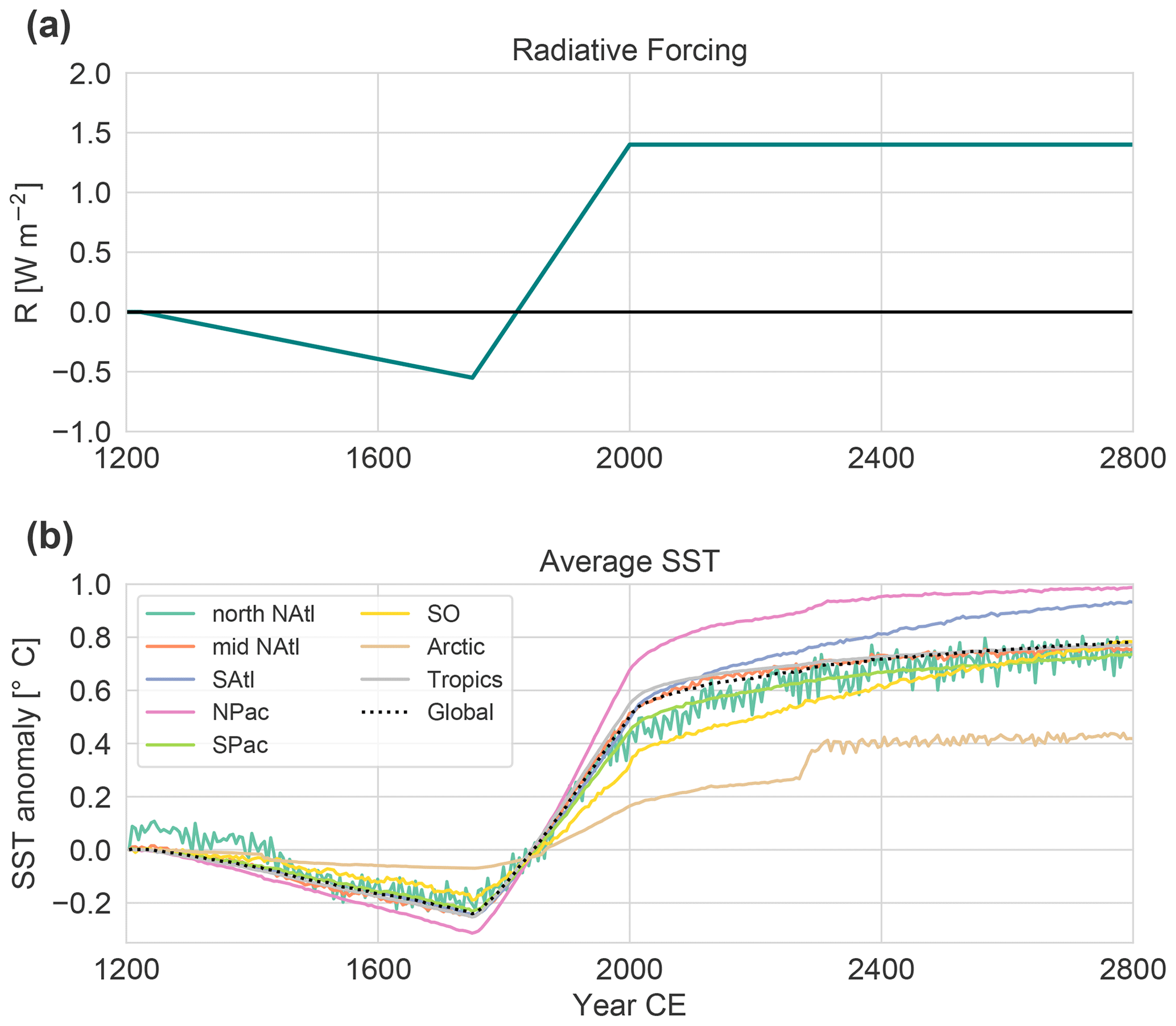
Figure 1(a) Idealized radiative forcing, which is used in the case of coupled simulations (OcAtmTRA and OcAtmFIX; see Table 1). (b) Sea surface temperature anomaly as a result of the forcing in (a): globally (black, dotted line) and averaged per region (colours, defined in Fig. A1). The global average SST at 1200 CE is 18.0 ∘C.
While the exact radiative forcing is of lesser relevance here, we note that the global average SST anomalies are comparable with reconstructions (PAGES 2k Consortium, 2013; Rayner et al., 2003). Our global SST anomaly shows a cooling amplitude of −0.24 K followed by a +0.74 K warming until 2000 CE (Fig. 1b) and approximately follows the SST variations reported by Gebbie and Huybers (2019) (−0.27; +0.87 K; from their Fig. 1a), which are in turn based on proxy reconstructions from the PAGES 2k Consortium (PAGES 2k Consortium, 2013) before 1950 CE and instrumental data from HadISST after 1870 CE (Rayner et al., 2003). For the overlap period (1870–1950), Gebbie and Huybers (2019) take a weighted linear combination of the two such that their resulting warming amplitude (+0.87 K) is higher than the proxy-only signal (PAGES 2k Consortium, 2013: +0.53 K), because the instrumental data exhibit a larger amplitude of industrial warming.
2.3 Simulations with fixed and transient ocean circulation
Quantification of the influence of changing ocean circulation on the tracer distributions of temperature and salinity is not trivial, because temperature and salinity are “active” tracers, which influence the ocean circulation through changes in density. We disentangle the effects caused by changes in the surface values from those caused by circulation changes by requiring for every experiment two simulations: one in which the ocean circulation adjusts transiently to the buoyancy distribution and one in which the circulation is kept constant; both are forced with identical surface boundary conditions.
Simulations with fixed ocean circulation are implemented by using diagnosed values of the density at every grid cell from one annual cycle at steady state. The velocities in x, y and z directions follow from frictional geostrophic and hydrostatic balance. Therefore, the circulation, including advection, diffusion and convection, is maintaining a perpetual seasonal cycle and does not respond to SST changes impacted by atmospheric changes at the ocean surface. Note that unphysical effects could arise, e.g. when convection still operates, although the water column at that location could now be stably stratified. This approach allows us to isolate the effect of changing ocean circulation by taking the difference between a transient and a fixed run under the same boundary conditions. This is realized by a series of ocean-only simulation pairs, summarized in Table 1.
Table 1Simulations performed in this study.

a Simulations are either run using the coupled Bern3D (with radiative forcing in the atmosphere as in Fig. 1a) or as ocean-only Bern3D (prescribed SST, SSS and sea ice from OcAtmTRA or OcAtmTRALong). b Ocean circulation can be fixed or transient, i.e. responding to SST and SSS changes. c In sensitivity simulations, the mixing parameter KD (diapycnal diffusivity) and wind stress τwind are varied.
Crucial to our approach is that these boundary conditions must be identical at the atmosphere–ocean interface and not, for example, at the top of the atmosphere. When we use the fully coupled Bern3D with transient ocean circulation (OcAtmTRA) and with fixed circulation (OcAtmFIX; not used elsewhere) under the same radiative forcing, the resulting two simulations possess different SST and SSS patterns, because ocean–atmosphere feedbacks differ between the transient and fixed case, as was already suggested by Garuba and Klinger (2016). These SST differences are small, but of the same order of magnitude as the changes in deep ocean temperature, and would therefore mask the signal we want to detect. We resolve this by running the model in an ocean-only mode that is forced with the same SST, SSS and sea ice in both transient and fixed simulations. The possibility to run the Bern3D model under time-varying surface boundary conditions has been newly implemented for this study. For every time step of the 1600 simulation years, the SST, SSS and sea ice of surface grid cells are set to the corresponding value in the (latitude, longitude, time step) boundary conditions that are obtained from a previous coupled transient simulation OcAtmTRA over 1600 years (Fig. 1). All ocean-only simulations in Table 1 are run under identical surface boundary conditions saved from the OcAtmTRA simulation from the year 1200 to 2800 CE. The coupled and ocean-only models are forced with the same seasonally varying wind field climatology.
2.4 Steady state
The coupled simulations are run to equilibrium under pre-industrial conditions. When switching to the ocean-only configuration, a model drift is observed that requires an extension of the spin-up. The ocean-only model is run for another 5000 years using the steady state SST, SSS and sea ice distributions from a period of 100 years, repeated 50 times. Afterwards, the ocean-only simulations OcTRA and OcFIX are started. During the extended spin-up, adjustments of the global ocean circulation take place: the steady state Atlantic meridional overturning circulation (AMOC) maximum decreases by 1.5 Sv and the strength of the global meridional overturning circulation (MOC) decreases by 0.8 Sv. Deep ocean temperatures are 0.3 to 0.6 ∘C colder below 3 km, because of a relative increase in Antarctic Bottom Water (AABW) with respect to North Atlantic Deep Water (NADW), and are up to 0.2 ∘C warmer in the depth range from 500 to 3000 m due to an absolute decrease in NADW. By the end of this additional spin-up, the residual drift of basin-mean ocean temperature at 3 km depth during the last 500 simulation years is less than K yr−1 in the Pacific and less than K yr−1 in the Atlantic. Sensitivity simulations with varying mixing and wind stress require their own steady state. For each of these four simulation pairs, we perform a similar 5000-year ocean-only spin-up, but with the respective parameter values given in Table 1.
3.1 Circulation change
Figure 2 shows the responses of the MOCs in the Atlantic (AMOC), the Indo-Pacific (IPMOC) and the Southern Ocean (SOMOC) for the ocean-only simulations forced by the imposed surface fields during the 1600 simulation years. Maxima and minima are evaluated below a depth of 400 m in order to avoid shallow Ekman-driven overturning cells. The Atlantic, Pacific and Indian basins are defined as being between 35∘ S and 70∘ N, and the SO extends southward of 35∘ S throughout this study, unless indicated otherwise. By design, the circulation is constant over time in the fixed case. During the medieval cooling, the AMOC increases slightly by ∼0.2 Sv, whereas the negative IPMOC and SOMOC both strengthen by ∼0.7 Sv. Industrial warming starting in 1750 causes the AMOC to slow down by 1.5 Sv, whereas both the IPMOC and SOMOC weaken by about ∼2.2 Sv until 2000. This 1.5 Sv AMOC slowdown is within the 1σ CMIP5 range of fully coupled AOGCMs under low emission forcing (Collins et al., 2019). After 2000, the AMOC maximum recovers under the constant forcing with a relaxation timescale of about 470 years, whereas the IPMOC takes significantly longer to reach equilibrium, and for this case a well-constrained timescale cannot be determined from the present simulations. The SOMOC does not recover but weakens by an additional ∼1.3 Sv over the final 800 years.
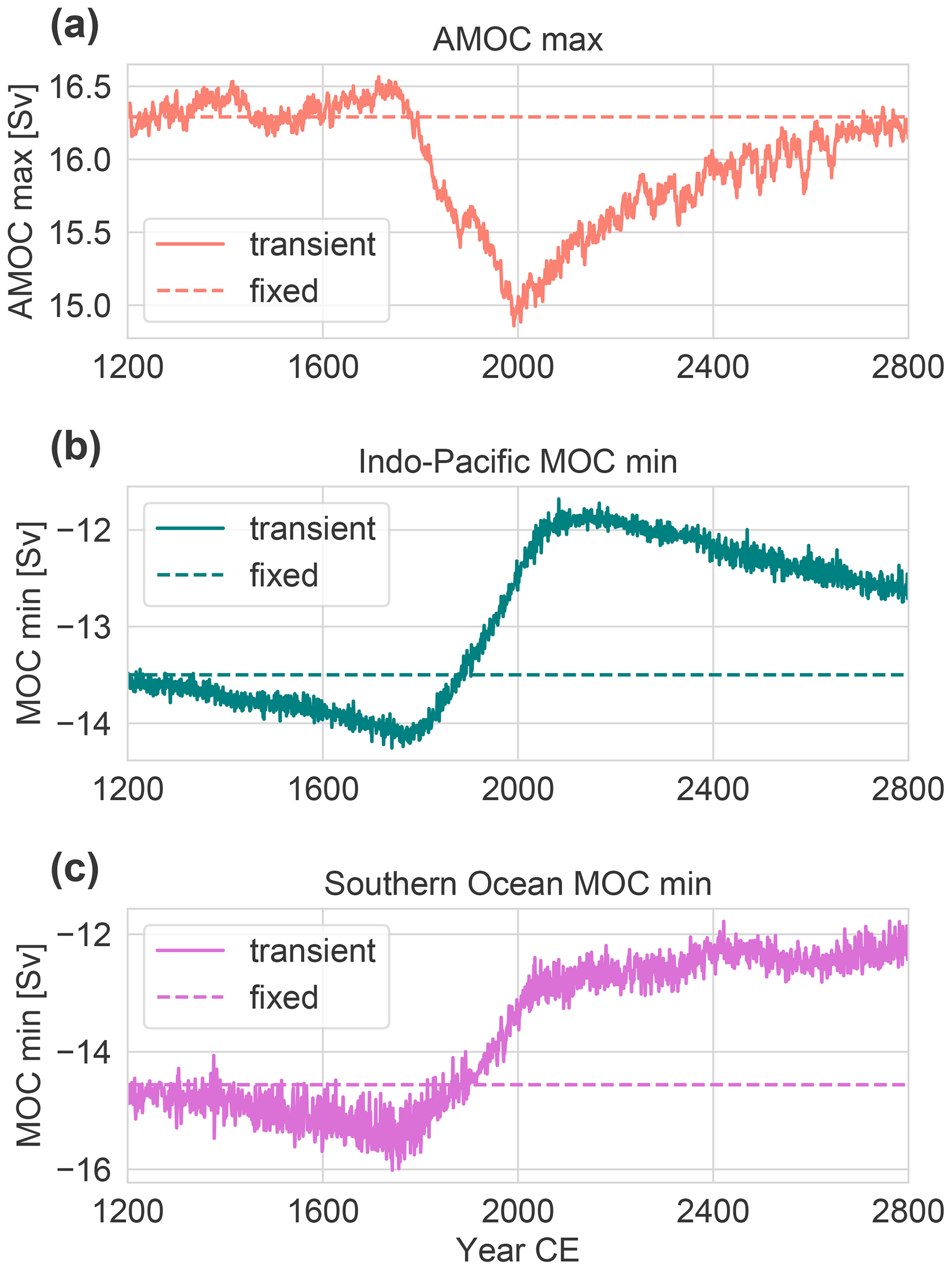
Figure 2Response of the maximum and minimum values of the meridional overturning circulation (MOC) to imposed SST, SSS and sea ice (Fig. 1b). (a) Atlantic MOC maximum, (b) minimum of the MOC in the combined Pacific and Indian basins (IPMOC) and (c) in the Southern Ocean (SOMOC). Simulations OcTRA (transient) and OcFIX (fixed) are shown.
The overturning stream functions are shown in Fig. 3 at 1205 CE as well as their anomalies in the years 1750 and 2000 CE (simulation OcTRA). The AMOC deepens during the medieval cooling phase, which leads to an increase of about 0.8 Sv at 2 km depth, although the maximum AMOC increased by only ∼0.2 Sv by 1750 (Fig. 2a). The largest changes of the AMOC occur during the industrial warming at depths of 2 km by reaching up to 2 Sv, and the reduction of overturning occupies the entire Atlantic ocean basin from 1 to 3 km depth. IPMOC changes are primarily located in the Southern Hemisphere with a strengthening of the circulation below 3 km at the southern margin of the basin during the medieval cooling, and a subsequent weakening above 3 km. The global MOC shows a strong bipolar response to the medieval cooling and industrial warming. That is, the absolute value of MOC strength increases in both hemispheres from 1205 to 1750, and a subsequent opposite and stronger response is simulated during the industrial warming.
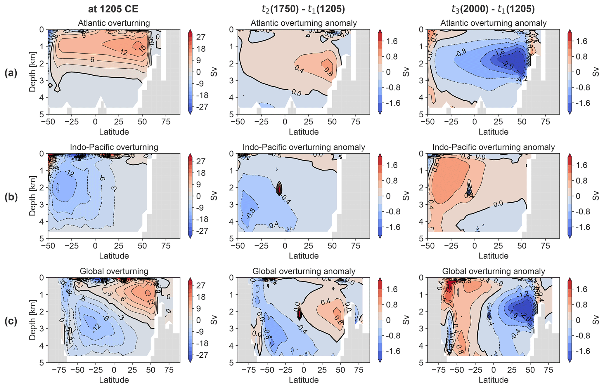
Figure 3Meridional overturning circulation for the transient ocean-only simulation OcTRA for (a) the Atlantic (AMOC), (b) the Indo-Pacific (IPMOC) and (c) globally at different time steps: at the start (1205 CE) and the anomalies at the coldest point of the Little Ice Age (1750 CE) and in 2000 CE. Values are averages over 15 years (for 1205–1220 CE) and 30 years (around 1750 and 2000 CE). Note the changing colour bar and latitude axis. The overturning stream function is positive (red) for water rotating clockwise and negative (blue) for water rotating anticlockwise.
3.2 Propagation of temperature anomalies into the deep ocean
We now turn to the propagation of the atmospheric temperature anomaly into the deep ocean. Figure 4a and b show Hovmöller diagrams illustrating the development of the basin-averaged temperature anomalies as a function of depth for each ocean basin. Temperature anomalies are small and reported here in units of centi-Kelvin (1 cK = 10−2 K). The propagation of the LIA cooling into the deep ocean is clearly visible, followed by the industrial warming signal. Qualitatively distinct patterns for the transient (TRA) and fixed (FIX) circulations emerge in all basins with a generally faster and stronger transfer of the anomalies to the deep ocean in the TRA case. However, local differences appear, particularly in the Atlantic Ocean. For TRA, the deep Atlantic shows an isolated cold anomaly at about 3 km depth, which develops by the end of the medieval cooling period and persists for several centuries. This feature, observed in the more realistic TRA simulation, suggests that the cold anomaly created by the pre-industrial cooling can be detected long into the future. It is evident that this anomaly is a result of the changes in MOC, as the fixed circulation case does not exhibit this isolated anomaly. In the year 2000 in TRA, the cooling is still strong and occurs below 2.5 km depth in the Atlantic, whereas for FIX much weaker cooling is confined to below 3 km. On the other hand, in the Pacific basin, where the MOC changes during the warming are generally smaller, the signal propagation into the deep ocean is rather uniform and follows the surface forcing with a delay due to ocean circulation. Here, the faster signal transfer to further depths in TRA is particularly evident. The SO also shows a uniform signal propagation with a faster transfer in TRA.

Figure 4(a, b) Hovmöller diagrams of temperature anomalies in centi-Kelvin (1 cK = 10−2 K) over depth. Values are basin averages of the Atlantic or Pacific (35∘ S–70∘ N) or the Southern Ocean (<35∘ S). Colour levels increase in steps of 5 cK from −20 to 20 cK and in steps of 10 cK otherwise. Red lines track the minimum temperature anomaly and indicate where the temperature trend changes from cooling to warming. (c) The lag in occurrence of the transient minimum temperature anomaly with respect to the fixed anomaly. This equals the red line in (a) minus the red line in (b). (d) Temperature anomalies from (a, b) are repeated for a fixed 3.1 km depth. Pink and green arrows indicate lags (positive) and leads (negative) of the transient with respect to fixed simulation in the temperature trend change at this depth (also indicated in c). Results are for simulations OcTRA (transient) and OcFIX (fixed).
In the Atlantic, the more effective downward propagation of negative temperature anomalies in TRA is linked to water mass changes in the proportion of AABW versus NADW, as AABW water is about 3 ∘C colder than NADW. At the end of the simulation (2800 CE), relatively more cold AABW at the expense of NADW is observed at depths from 2 to 4 km, which correspond to the location of the persistent cold anomaly. This is illustrated by dye tracers tracking AABW and NADW in Fig. A3. The opposite (an increase in NADW at the expense of AABW) occurs above 2 km and below 4 km, explaining the stronger Atlantic warming in TRA at these depths. In the Pacific, the more effective downward transport in TRA is explained by increased inflow of deep southern water during the cooling, and afterwards the positive IPMOC anomaly causes less inflow of cold AABW during the subsequent warming and hence a more effective warming at depth in TRA than in FIX (see Fig. 3). The SO is already warming in the year 2000 for both TRA and FIX, because of its high ventilation rate. This ventilation rate in the SO (Figs. 8d and 9d) agrees well with radiocarbon-based observations (Gebbie and Huybers, 2012) in the average and maximum SO water age, although qualitatively the Bern3D deep water formation occurs too far south (since it is enhanced with a prescribed salt flux in the Ross and Weddell seas).
The red lines in Fig. 4a and b track the minimum temperature anomaly at every depth. This helps us identify whether the deep ocean at present (2000 CE) is still cooling (red line to the right of vertical line) or already warming. Leads and lags of the temperature minimum of the two simulations FIX and TRA can be readily determined. Figure 4c provides the depth dependence of the lag of the temperature minimum in TRA with respect to that in FIX. The temperature minimum in TRA in the Pacific and the SO appears earlier, and this lead grows up to 150 years at depth. In the Atlantic, this structure is interrupted by a strong lag between 2.5 and 4 km of over 200 years. Hence, changing circulation accelerates the propagation of the downward signal everywhere except in the Atlantic between 2.5 and 3.5 km depth, providing a mechanism for ocean memory of past changes in surface climate. In Sect. 4, we will carry out sensitivity tests to assess the robustness of our findings.
Figure 4d presents the time series view of temperature anomalies at 3.1 km, the depth where the strongest differences between the basins are found. Here, changes in ocean circulation delay the arrival of industrial warming by more than 200 years in the deep Atlantic, whereas they accelerate the arrival by about 120 and 150 years in the deep Pacific and deep SO, respectively. Another notable feature is that the amplitude is higher for TRA than for FIX in each basin. As discussed in Sect. 4, this is a robust feature. Similarly, Xie and Vallis (2011) found that changing ocean circulation increases the effective depth to which anomalous heat reaches under their warming experiments. They attribute this to changing circulation allowing for more heat uptake via (a) reducing average SST and (b) reducing surface heat loss at high latitudes.
3.3 Decomposition of temperature anomalies
Anomalies of the transport of a quantity Q=Q(x, y, z), vQ, in the ocean can be decomposed into contributions originating from changes in transport velocity v and in the quantity itself. Following Winton et al. (2013), we write
where Q0 and v0 are the steady state values of the quantity Q and the transport velocity v (including advection, diffusion and convection), and Q′ and v′ are their deviations. Here, Q can be any quantity transported in the ocean, e.g. temperature, salinity, heat. We consider the heat content density:
where Cp=3981 J kg−1 K−1 is the specific heat capacity, ρ0=1027 kg m−3 is the reference water density obtained from the average seawater density in steady state, and T is the potential temperature. With Q as heat content density, the first term on the right hand side of Eq. (1) represents the steady state heat transport, and the second and third terms, v′Q0 and v0Q′, quantify anomalous heat transport due to changes in circulation and in SST, respectively. The last term is quadratic in the deviations and hence small. Based on an analysis of global means in a climate change experiment with a 1 % per year increase in CO2 and evaluated for the year 100, Winton et al. (2013) give an estimate of .
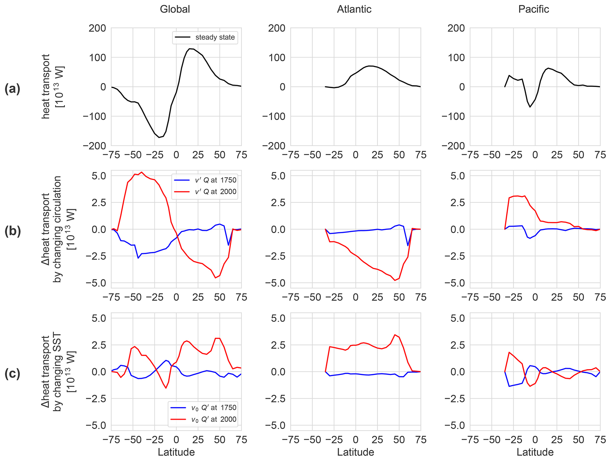
Figure 5(a) Global and basin northward meridional heat transport in the ocean at steady state, OcFIX (t=1200). Meridional heat transport anomaly due to (b) changing circulation and (c) changing SST. The coldest time of the LIA is shown in blue (1750 CE) and the industrial warming phase in red (2000 CE). Note the different order of magnitude on the y axis. Results are derived from simulations OcTRA and OcFIX (see text) and variables v and Q refer to Eq. (1).
We can find the contribution of each term in Eq. (1) by making use of experiments OcTRA () and OcFIX (): v0Q0 is calculated from OcTRA or OcFIX for the year 1200; v′Q from the difference between the two, i.e. OcTRA – OcFIX; and v0Q′ results from the difference of OcFIX and its steady state, i.e. OcFIX – OcFIX (t=1200). The sum of all these indeed corresponds to OcTRA, which equals vQ. As mentioned by Winton et al. (2013), it is not possible to separate the terms , because the model only exhibits changing circulation v′ under , as otherwise surface density is unchanged. A difference between this study and Winton et al. (2013) is that in our set-up Q′ is the same for fixed and for transient simulations, since it is determined by the prescribed SSTs, which are identical for OcFIX and OcTRA.
The decomposition of the northward global heat transport vQ is shown in Fig. 5. The response of the meridional heat flux during the medieval cooling occurs primarily in the Southern Hemisphere and is caused by a strengthening of the circulation in the SO and Indo-Pacific and hence a stronger southward heat transport with only small changes in the Atlantic basin. The industrial warming is characterized by a decreasing poleward heat flux in both hemispheres. In the south, this is primarily due to changes in the Pacific circulation and changing SST and circulation in the SO. In the Northern Hemisphere, the weakening poleward heat transport is due to changes in the Atlantic Ocean. Here, changing circulation dominates in the form of a weakening overturning, which is only partly compensated by anthropogenic warming of the upper ocean.
We compare the meridional heat flux anomaly due to changing circulation during the industrial warming phase (Fig. 5b) to Winton et al. (2013) (their Fig. 5: bottom, black line). The shape of this redistribution heat transport in our Fig. 5b is comparable to Winton et al. (2013), but it is about an order of magnitude smaller. The warming experiment of Winton et al. (2013) is driven by a 1 % CO2 increase per year for 100 years, which corresponds to a radiative forcing of 4.5 W m−2, whereas the radiative forcing in our experiment is only 1.4 W m−2. The redistribution heat transport could also be smaller in our case because atmospheric processes are better represented in GCMs (general circulation models), such as the GFDL model used in Winton et al. (2013). The hydrological cycle of the Bern3D EMIC model reacts too weakly compared to another GCM, CESM version 1.0.1, for an ensemble member over the past millennium. Here the Bern3D SSS anomalies were an order of magnitude too low, although showing the same qualitative patterns.
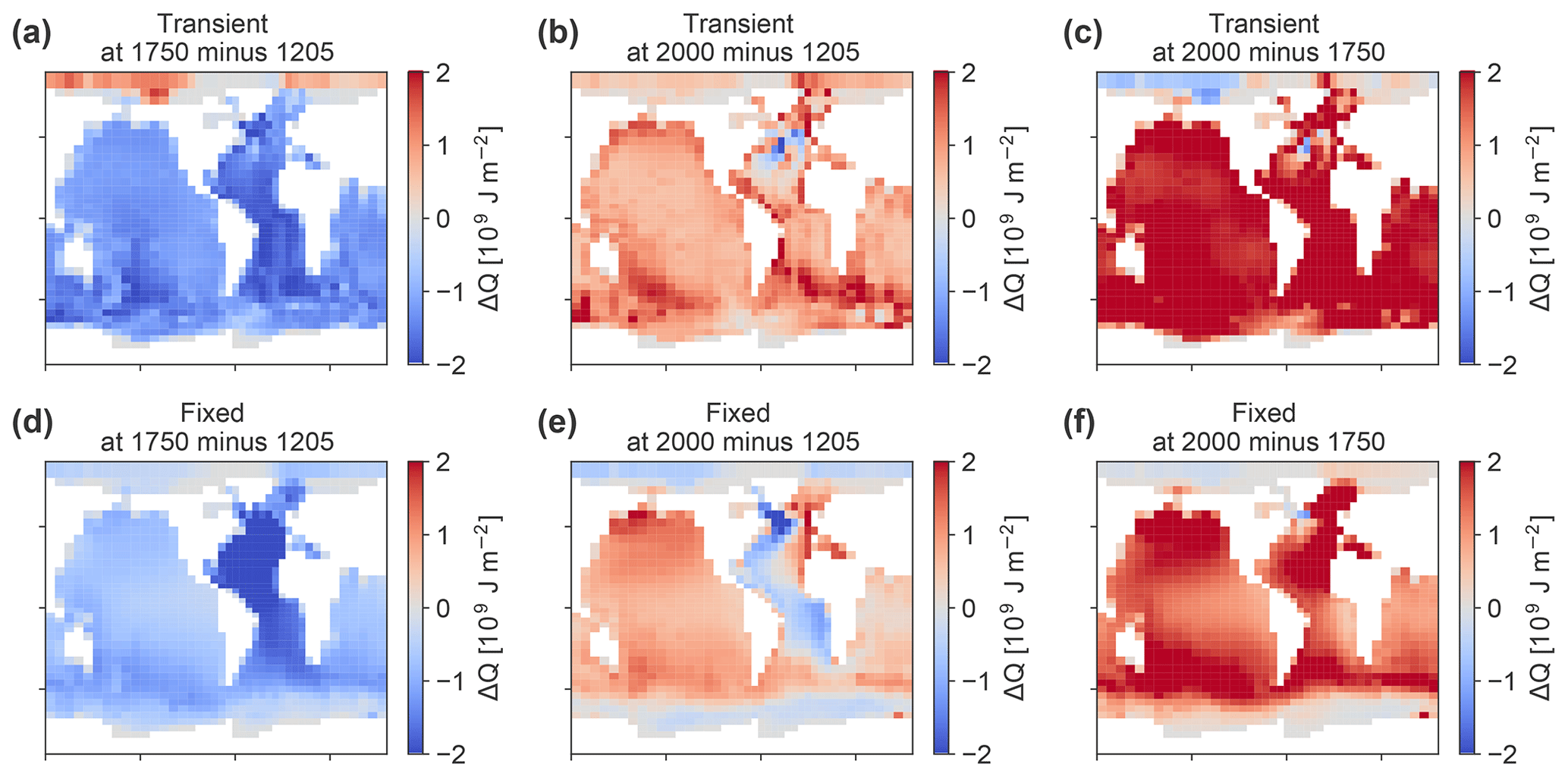
Figure 6Ocean heat areal density (OHD) anomalies for transient and fixed circulation. (a, b) Anomalies in 1750 and 2000 CE, both with respect to the year 1205 for case OcTRA and (d, e) for case OcFIX. (c, f) Anomalies in 2000 CE are also shown with respect to year 1750.
In addition to heat transport, the column-integrated heat content density per unit area, hereafter called ocean heat areal density (OHD), informs about the distribution of heat uptake. OHD is given as
where H is the total height of the water column. OHD anomalies in the years 1750 and 2000 are shown in Fig. 6. The medieval cooling causes a decrease in OHD globally (except in the Arctic in TRA), with relatively homogeneous cold anomalies in TRA, whereas FIX possesses the strongest cooling in the Atlantic in the year 1750. For FIX, the 550 years of cooling were not enough to reach the old waters in the deep Pacific, but in TRA stronger Pacific anomalies are caused by circulation changes, which overlay the steady state transport of anomalous heat. In 2000 CE compared to 1205 CE (Fig. 6b and e), FIX still bears the signature of the LIA in the Atlantic, Arctic and SO. In TRA, this heat deficit has disappeared with the exception of a small region in the North Atlantic. It is evident that the transient response of the circulation determines the magnitude and regional distribution of the memory of past sea surface temperature anomalies.
Comparing OHD in 2000 to 1750 CE instead (Fig. 6c and f), and hence only considering anomalies during the warming period, gives a different picture. All heat anomalies are much larger, since the LIA cooling is not subtracted in this case. In TRA the OHD anomalies are larger than in FIX, confirming once more our finding that signals are propagating more effectively, i.e. with a larger amplitude, into the ocean in TRA than in FIX. Further, hardly any negative anomalies are present anymore in TRA and FIX in 2000 when taken with respect to 1750. That is, the warming hole in TRA (Fig. 6b) mainly originates as a residual from the 1200–1750 LIA cooling and is not due to the AMOC slowdown from 1750 to 2000 in our ocean-only setting.
The global ocean heat content (OHC) is given by . The contributions of circulation and SST changes are determined by taking the difference between OcTRA and OcFIX respectively, taking the anomalies of OcFIX with respect to its steady state. The result is given in Fig. 7. The decrease in OHC during the LIA is clearly dominated by changing SST, which globally has an effect about 3 times larger than changing circulation. During the warming, changing circulation and changing SST have a similar influence on a global scale with a slight dominance of the former before about 2300 CE; afterwards changing SST takes over to some extent, because the effect of changing circulation decreases with recovering AMOC. The time evolution of the partitioning of OHC into circulation- and SST-related anomalies is different in the two basins (Fig. 7b and c). The medieval cooling of OHC is completely dominated by SST changes in the Atlantic, whereas the Pacific features an about equal contribution of circulation- and SST-related changes. The two effects contribute significantly in both basins under industrial warming, with a larger component of changing SST in the case of the Atlantic. As expected, changing SST contributes in both basins to an OHC decrease under LIA cooling and an increase under global warming. In contrast, changing circulation has an unexpected effect in the case of the Atlantic under the LIA cooling: it slightly counteracts the global cooling. This is also visible in Fig. 6, where the Atlantic cooled more in OcFIX (Fig. 6d) than in OcTRA (Fig. 6a).
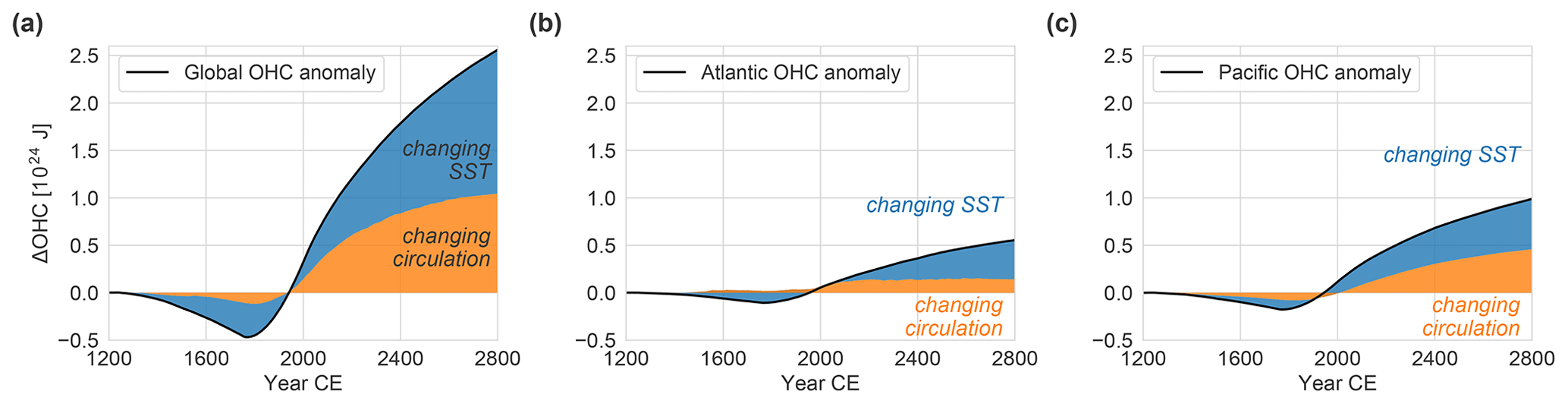
Figure 7Ocean heat content anomaly decomposed in contributions due to changing SST and due to changing circulation for (a) the global ocean, (b) the Atlantic and (c) the Pacific basin, derived from simulations OcTRA and OcFIX.
In this section, we have decomposed heat transport and OHC into the contributions of changing circulation and changing SST. Recall that the Hovmöller diagrams in Fig. 4a and b presented basin-averaged temperature anomalies over depth. These temperature anomalies, which are directly related to OHC (Eq. 3), can readily be decomposed as well: the OcFIX anomalies in Fig. 4b already equal the contribution of changing SST, and the contribution of changing circulation is found by subtracting column OcFIX from OcTRA. The result (Fig. A2) confirms that changing SST causes the expected downward propagation of cooling and warming, whereas changing circulation causes the persistent cold anomaly in the Atlantic around 3 km depth with an enhanced warming above and below this depth in addition to an enhanced warming after 2000 CE in the Pacific and SO.
3.4 Explaining the leads and lags
Now we turn our attention to deep ocean temperature and the effects acting on it in a more local framework: our aim is to gain more understanding of the leads and lags that we observed at 3.1 km depth in the different basins in Fig. 4. We distinguish two effects that influence deep ocean temperature: (1) the history of SSTs and (2) changing circulation, which we now split in two subeffects: (2a) shifts in water mass distribution, which determine where regional SST anomalies are carried, and (2b) the absolute overturning rate, i.e. how fast deep ocean water is replenished. In this section, we discuss these effects qualitatively with the help of Figs. 1b, 8 and 9. In Sect. B, rough quantitative estimates of these effects are computed (results in Table B3; interpretation in Sect. B5).
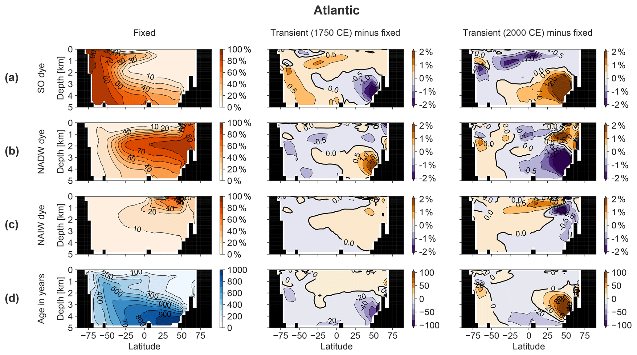
Figure 8Zonally averaged meridional section of the Atlantic basin, including the SO sector, showing (a) Southern Ocean dye tracer, (b) North Atlantic Deep Water dye tracer, (c) North Atlantic Intermediate Water dye tracer and (d) ideal age. Columns show the fixed-circulation simulation (OcFIX) and the anomaly of transient (OcTRA) with respect to fixed dye tracer in 1750 (coldest time in LIA) and 2000 CE. Units for dye are a fraction of initial dye concentration at the surface, in percent.
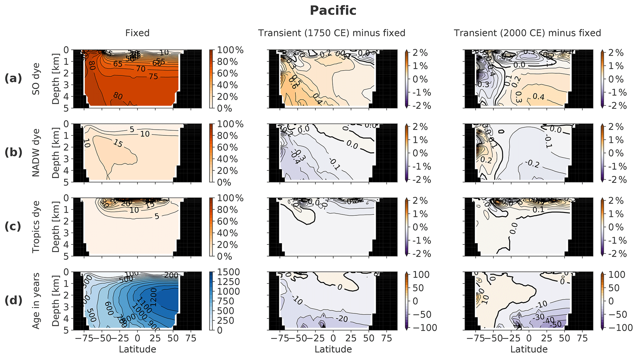
Figure 9Zonally averaged meridional section of the Pacific basin, including the SO sector, showing (a) Southern Ocean dye tracer, (b) North Atlantic Deep Water dye tracer, (c) tropics dye tracer and (d) ideal age. Columns show the fixed-circulation simulation (OcFIX) and the anomaly of transient (OcTRA) compared to fixed dye tracer in 1750 (coldest time in LIA) and 2000 CE. Units for dye are a fraction of initial dye concentration at the surface, in percent. Colour levels for Pacific anomalies increase in steps of 0.1 % dye or 10 years of age.
Firstly, historical SST anomalies differ between regions such that deep water formation regions experience different surface temperature trends. As an illustration, we refer back to Fig. 1b for our idealized forcing. Recall that regions are defined in Fig. A1 and correspond to the source regions of different dye tracers. We notice relatively high amplitudes in the North Pacific and South Atlantic, and low amplitudes in the Arctic, but these regions play a minor role in determining the ocean temperature at depth. The larger variability of northern North Atlantic SST is due to convection occurring in only 40 grid cells there. This region's SST (NADW formation) sees no clear cooling during the first two centuries but catches up with the global average cooling trend afterwards. The Southern Ocean SST (AABW and AAIW) starts cooling rapidly, but with a smaller amplitude than the global average. Comparing these two most important water masses, we conclude that NADW sees less of the LIA cooling than AABW during 1200–1400 CE, but more during 1500–1750 CE.
Let us turn to effect 2a, shifts in the distribution of water masses, which are illustrated by means of dye tracers. The meridional distribution of the water masses that dominate the abyss is shown in Fig. 8a–c (Atlantic) and Fig. 9a–c (Pacific). We track the combined water masses of AABW and Antarctic Intermediate Water (AAIW) with one Southern Ocean dye. First we discuss the changes in 1750: the largest water mass changes occur in the North Atlantic at 3 km depth, where the NADW fraction increases by about 2 percentage points at the expense of AABW (3 ∘C colder than NADW). This has a warming effect that counteracts the LIA cooling in the Atlantic. In the deep Pacific, however, slightly more AABW flows in from the south at the expense of NADW. Analogously, this has a cooling effect and enlarges the propagation of the LIA cooling in the transient case. In the year 2000, dye tracers in the Atlantic reveal a pattern that is opposite to 1750, so they track a cooling at 3.1 km depth. In the Pacific (excluding the SO sector), the same qualitative water mass anomalies as in 1750 are still present, but displaced northwards. This slower water mass renewal is due to the longer residence time of waters in the Pacific. Opposite trends are developing in the SO. This is because of a delay: the amount of SO water mass is already decreasing in 2000 (and NADW increasing) but the decrease initiated only around 1900 CE, such that the water mass anomaly built up over 1200–1900 CE is not compensated for yet (not shown).
Effect 2b is the absolute overturning rate, estimated by changing water age. In principle it is possible that the rate at which water masses refresh would change without any change in the relative composition of water masses. For instance, AABW and NADW would then still be present in the same proportion, but a general speed-up of the circulation (a faster overturning) would make the water age younger. Intuitively, a strengthening of the global MOC brings more cold polar surface water to the abyss resulting in a global cooling of the deep ocean, because downward heat diffusion from low-latitude surfaces is opposed by upwelling of colder deep water. From the ideal water age in 1750 CE in Figs. 8d and 9d, we see that the water becomes younger by up to ∼40 years in the deep Atlantic and up to ∼10 years in the deep Pacific at 3 km depth. In 2000 CE, the age anomalies are in the other direction, as expected: the deep North Atlantic ages by more than 100 years, whereas the Pacific SO becomes ∼5 years older. The rest of the Pacific continues to become younger, which is again due to a delay, and the water will become older, with respect to 1200 CE, in 2100 CE (not shown). We conclude that effect 2b causes the deep Atlantic to see an older, and hence warmer, signal during the LIA cooling and a younger, and hence colder (noting that the ∼500 yr old water in 2000 CE still sees SSTs of 1500 CE), signal during the warming period after 1750. This contributes to a delay during both periods. We expect that the influence in the Pacific and SO is minor because of the small changes in age. This is confirmed by Sect. B5, which states that effect 2b only has an impact that is significantly non-zero in the case of the Atlantic in 2000 CE, in which case it indeed leads to a strong cooling. This effect 2b is even the main cause of the persistent cold anomaly in the deep Atlantic (Fig. A2a): estimated as 48 % in addition to 32 % of the cooling by effect 1 and 19 % by effect 2a.
Summarizing the above and Sect. B, we can explain the strong lag, i.e. persistent cold anomaly, in the deep Atlantic (Fig. 4d). Here SST and water mass changes counteract each other in 1750: they contribute roughly equally but with opposite signs, causing this significant delay in the arrival of the LIA cooling. In the year 2000, the effect of water ages comes into play and together with changing water masses now strongly enhances the amplitude of the cooling, which arrives relatively late. In the Pacific and SO, no counteracting effects are observed. SST and water mass changes both contribute a cooling such that the arrival of the LIA at depth is fastened and enhanced, which explains the observed leads and the larger amplitude for TRA.
The leads and lags of temperature minima from the LIA cooling (Fig. 4c and d) are determined by model-dependent changes in circulation, including advection, diffusion and convection. In this section, we test how robust the leads and lags are under varying key model parameters for mixing and wind. We run additional transient and fixed simulations with halved and doubled mixing and wind stress, respectively (Table 1). The changes are applied globally and uniformly. Figure 10 summarizes the resulting leads (negative) and lags (positive) throughout the water column of TRA with respect to FIX simulations.
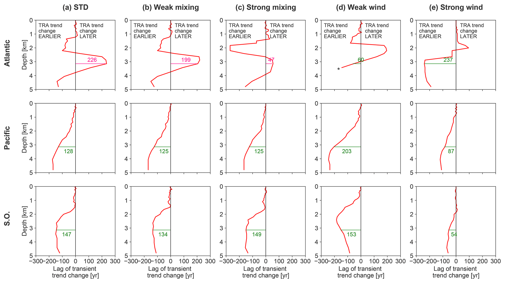
Figure 10Lags (positive) or leads (negative) in the arrival of the warming at each depth (transient minus fixed simulation). Results are shown for (a) the standard simulations OcTRA and OcFIX (repeated from Fig. 4c), (b, c) simulations with varying mixing (OcTRA_weakmix and OcFIX_weakmix in b and OcTRA_strongmix and OcFIX_strongmix in c) and (d, e) varying wind stress (OcTRA_weakwind and OcFIX_weakwind in d and OcTRA_strongwind and OcFIX_strongwind in e). Numbers indicate the values of leads and lags at 3.1 km depth. * For (d), the red line stops in the Atlantic below 3.4 km, because the LIA cooling anomaly is not detectable in OcFIX_weakwind at these depths such that its trend change is undefined.
An overall picture appears of leads in the Atlantic that are interrupted by a depth range of lags, and leads throughout the Pacific and SO. These lags in the Atlantic are located between about 2.5 and 4 km for standard, weak mixing and strong mixing simulations, but they are shifted upwards for weak and strong wind, from 1.5 to 3 km and from 1.5 to 2 km, respectively. Therefore, our finding that changing circulation delays the propagation of the downward signal in a certain depth range in the Atlantic but accelerates it everywhere else is robust, with the precise depth range boundaries depending on model parameters.
At a fixed 3.1 km depth, the leads and lags are relatively robust under varying mixing, but not under varying wind, especially in the Atlantic. The diapycnal diffusivity KD is halved or doubled to vary mixing (Fig. 10b and c). In the Atlantic, weak mixing does not have much influence, but strong mixing makes the ∼226 yr lag almost disappear. This is explained by the presence of two local temperature minima in the Atlantic for OcFIX (Fig. 4b), OcFIX_weakmix and OcFIX_strongmix. Only in the case of OcFIX_strongmix, the global minimum, which is marked to compute the lag, is shifted towards the second local minimum. A change in FIX compared to the standard simulation OcFIX is possible, since the steady states for weak and strong mixing are different (Figs. A4–A5). Lead times in the Pacific and SO stay within the range of 125 to 150 years and are hence insensitive to these rather large changes in KD. Steady states possess especially different MOCs for halved and doubled wind stress τwind. Increasing wind stress almost doubles the MOC in the Northern Hemisphere and creates a strong Deacon cell in the SO, i.e. Ekman-driven equatorward flow. This causes large differences in simulated leads and lags for varying wind (Fig. 10d and e). The lag in the Atlantic becomes a lead instead, whereas the leads in the Pacific and SO range from about 50 to 200 years.
For the standard simulation, amplitudes of LIA cooling were considerably larger in TRA than in FIX at 3.1 km depth, as noted previously in Fig. 4d. This property is robust under varying mixing and wind: all sensitivity simulations possess larger TRA than FIX amplitudes at 3.1 km in all basins, except strong wind in the Atlantic (not shown). Thus, circulation changes enhance the amplitude, and hence detectability, of deep ocean temperature anomalies.
Our study was motivated by the earlier study of Gebbie and Huybers (2019) (GH19, henceforth), who interpreted deep ocean temperature anomalies with an inverse model with fixed circulation, inferred from oceanographic measurements from the late 19th century and modern observations. Early transects in the Atlantic and Pacific oceans are available from the expedition of the HMS Challenger of 1872–1876, and modern data were obtained during WOCE in the 1990s. As a result, the circulation state in the model of GH19 corresponds well with observations and with measured ventilation rates. GH19 have identified coolings and warmings at a depth range of 1800 to 2600 m, which they attribute to remnant deep ocean signals of surface climate change. They find that the deep Pacific has been cooling during that period, but the deep Atlantic, particularly in the Northern Hemisphere, has been strongly warming.
We refer back to the basin-averaged Hovmöller diagrams in Fig. 4a and b. These compare directly to Fig. 1c and b from GH19, though with a different time axis: we show 1200–2800 CE, whereas they simulate 0–2000 CE, including a medieval warm period around 600 CE. The downward propagation of temperature anomalies in the Pacific qualitatively agrees between the two studies. The result of GH19 in the Atlantic is qualitatively similar to our FIX case but not to TRA, which is as expected since their model has a fixed circulation. This confirms again that the persistent cold anomaly in the deep Atlantic observed for the Bern3D TRA originates from circulation changes, i.e. from an increase in southern sourced water at this depth (Fig. A3). We expect that most models with transient circulation show this behaviour under AMOC slowdown, but the strength and timing of the persistent cold anomaly will be model-dependent. Quantitative amplitudes of deep ocean cooling until 2000 CE are similar in the Pacific in the two studies, but GH19 show slightly stronger cooling in the Atlantic (up to 20 cK instead of 15 cK), which also extends deeper.
Now we answer the question of whether in the simulations the deep ocean (2 km and deeper) at present is still cooling from the LIA or already warming. Recall that the red lines in Fig. 4a and b help us identify whether the deep ocean at present (2000) is still cooling (red line to the right of 2000) or already warming (red line to the left of 2000). GH19 predicted that the deep Pacific is still cooling at present, but the deep Atlantic is already warming. For the Pacific, this is consistent with our FIX case but not with TRA, which is thought to be more realistic than FIX. In our study, most of the deep Atlantic water column is still cooling at present for both TRA and FIX (although the 2–3 km part is already warming in FIX).
In addition, we reproduce Fig. 2 from GH19 (repeated in Fig. 11c) for the two cases of OcTRA and OcFIX (Fig. 11a and b), which focus on a depth of about 2 km. Note that in our TRA case it makes a significant difference which depth we consider, whereas their anomalies travel down more uniformly over depth. At 2 km depth, the fingerprint of circulation changes is not as strong as for instance at 3 km. Figure 11a and b show a widespread warming trend from 1875 to 1995 CE in both cases in the North Atlantic. However, both cases also exhibit a cooling trend during this time interval in some limited areas of the North Atlantic. For TRA, cooling is simulated in the northeast Atlantic, whereas FIX shows cooling in the northwestern part of the North Atlantic. In the Pacific, warming (TRA) or cooling (FIX) trends are very small. In our FIX simulation, a cooling trend is found in the Pacific, but it is rather weak, and the southwestern Pacific is warmer in 1995 compared to 1875 CE. The differences between Challenger and WOCE data, as well as the model simulation of GH19 (Fig. 11c), show a clear remnant cooling trend in the Pacific in this depth range around 2 km.
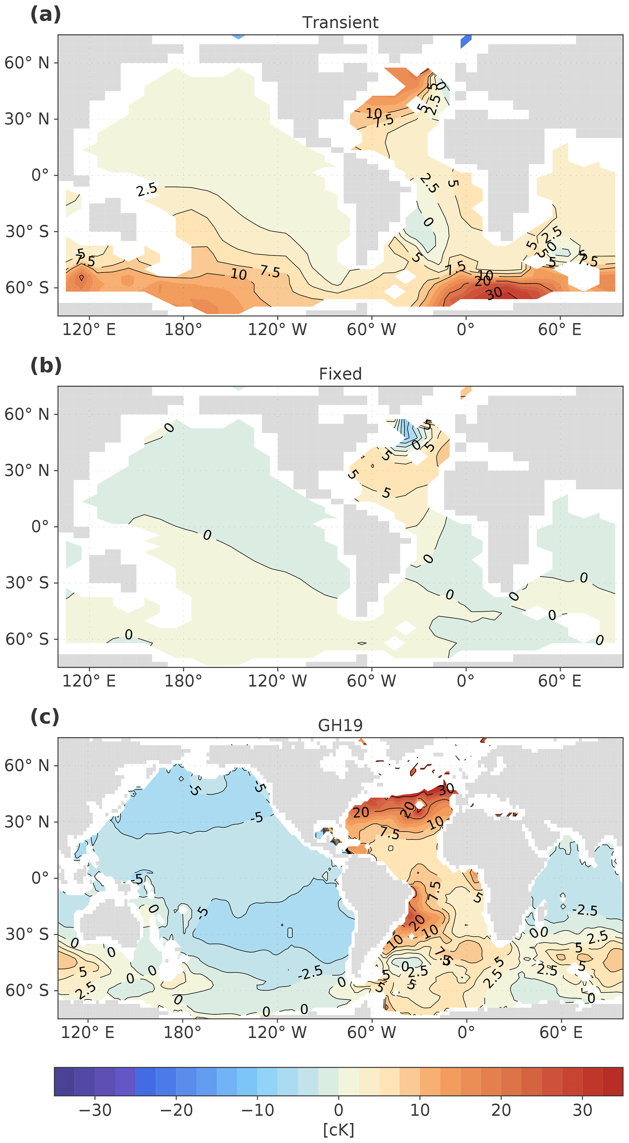
Figure 11Comparison with Fig. 2 of Gebbie and Huybers (2019) for the two cases of transient and fixed circulation. Deep ocean temperature anomalies are determined between 1872 and 1876 (Challenger expedition) and between 1990 and 2002 (WOCE campaign) and averaged over the depth of 1800 to 2600 m, for (a) simulation OcTRA (transient), (b) simulation OcFIX (fixed) and (c) the model output of Gebbie and Huybers (2019), Fig. 2, repeated here for easy comparison.
The fact that the deep Pacific cooling is weak in our simulations could be caused by the choice of our forcing, which is simpler than that used by GH19 with less climate fluctuations and has a slightly smaller industrial warming amplitude. We have ignored climate variations before the year 1200, whereas GH19 start at 0 CE and simulate an early medieval warm period before 1200. An additional Bern3D experiment (simulations OcTRALong and OcFIXLong) with a medieval warm period before 1200 (similar in amplitude to GH19) showed that this does not alter our main results. Figure A6a and b only show subtle differences compared to Fig. 4a and b from ca. 1600 CE onward. For example, the preceding medieval warm period delays the arrival times of the temperature minimum in the Atlantic between 2 and 3 km by only 10 (FIX) to 35 (TRA) years. A notable difference is also that the cooling in the Pacific no longer penetrates below 2 km for OcFIXLong (in the case of OcFIX the cooling here was less than 5 cK).
Understanding the evolution of deep ocean temperature brings insight into the ocean heat content and its rate of change and is important for the initialization of historical and present-day simulations. We found that even the relatively small changes in ocean circulation during the last 800 years have a profound impact on deep ocean temperature. While changing ocean circulation fastens the arrival of cold and warm atmospheric temperature anomalies in the deep Pacific and deep SO, it delays the arrival of this signal in the deep Atlantic between about 2.5 and 3.5 km depth. This lag in the deep Atlantic is two centuries in our simulations and is caused first by a relative increase in NADW at the cost of AABW during the LIA cooling, followed by an older water age under AMOC slowdown during industrial warming. Moreover, circulation changes enhance the amplitude of deep ocean temperature fluctuations in all three major basins, thus making atmospheric anomalies better detectable in the deep ocean.
We have decomposed heat transport and OHC anomalies into the contributions of changing circulation and changing SST. Poleward heat transport decreased under early industrial warming, in which the effect of changing circulation was dominating. Our second decomposition showed that OHC anomalies were for about one-third caused by changing circulation during the LIA cooling (hence two-thirds by changing SST), whereas both effects had an approximately equal contribution under industrial warming. We conclude that ocean heat uptake is not solely dominated by atmospheric temperature anomalies, but changing ocean circulation has a significant impact.
Lastly, we assessed the robustness of leads and lags under varying mixing and wind strengths. The transient simulation, where ocean circulation adjusts dynamically, still had a larger amplitude than the fixed-circulation simulation in almost all cases and basins. At the fixed depth of interest of 3.1 km, the circulation-caused leads in the deep Pacific and SO versus lags in the deep Atlantic were quantitatively quite robust under varying mixing, but not under varying wind stress. Throughout the water column, the qualitative result of leads in the Pacific and SO is robust under our sensitivity tests. The same holds for the interesting observation of leads in the Atlantic that are interrupted by lags at a certain depth range (either around 2 or around 3 km).
We are aware that our results are to a certain extent model-dependent and therefore we welcome more research concerning the propagation of past surface temperature anomalies to the abyss in other models. The modelled age of deep waters and the relative response of AMOC versus SOMOC strength under changing SST are especially important possible biases for this study. In the Bern3D model, the deep North Atlantic is too old compared to radiocarbon observations (Gebbie and Huybers, 2012), which correspond to the ages in the observation-based model of GH19. These observations show radiocarbon ages of up to 600 years in the North Atlantic (zonal average), whereas we find ideal ages over 900 years (Fig. 8). The sensitivity simulations with strong mixing have a smaller bias in North Atlantic water age (maximum age ca. 800 year) and still show a temperature propagation very comparable to Fig. 4 (not shown). We conclude that this model bias is likely not responsible for the main differences between GH19 and our study. Another weakness of the coupled Bern3D model is the representation of atmospheric processes, in particular the hydrological cycle. As such, the generated time-varying SSS field could be replaced in future work by a more realistic SSS from another coupled model or via paleoreconstructions (e.g. the PHYDA database of Steiger et al., 2018).
In this paper, we kept ocean–atmosphere feedbacks identical between transient and fixed simulations, by prescribing the same SST and SSS time series. We needed this for a correct comparison of the propagation of (identical) sea surface temperature to depth. In reality, ocean–atmosphere feedbacks and SST patterns are different when the ocean circulation is allowed to dynamically adjust, i.e. in transient simulations (Winton et al., 2013). These effects come on top of the contribution of changing circulation we found. It would be interesting to find a way to combine our approach with the approach of Winton et al. (2013) such that deep ocean temperatures can be compared in an unbiased way without losing the ability to study different ocean–atmosphere feedbacks.
In our case study of the past 800 years, we chose an idealized forcing, whereas Gebbie and Huybers (2019) used a forcing with more high-frequency SST fluctuations, which is more realistic but also harder to interpret. Moreover, one could use an even more realistic forcing by prescribing time-varying SST fields with trends that differ between regions, for example with different times of occurrence of the LIA, by obtaining them directly from recent paleoreconstructions (Neukom et al., 2019) instead of from the simulation OcAtmTRA. In a more general view, we would be able to understand how any historical SST record travels down to the deep ocean when we understand the effective depth to which surface temperature anomalies travel (Xie and Vallis, 2011) as a function of the anomaly's frequency and amplitude, and depending on changes in ocean circulation that are a response to this cooling or warming.
A1 General figures
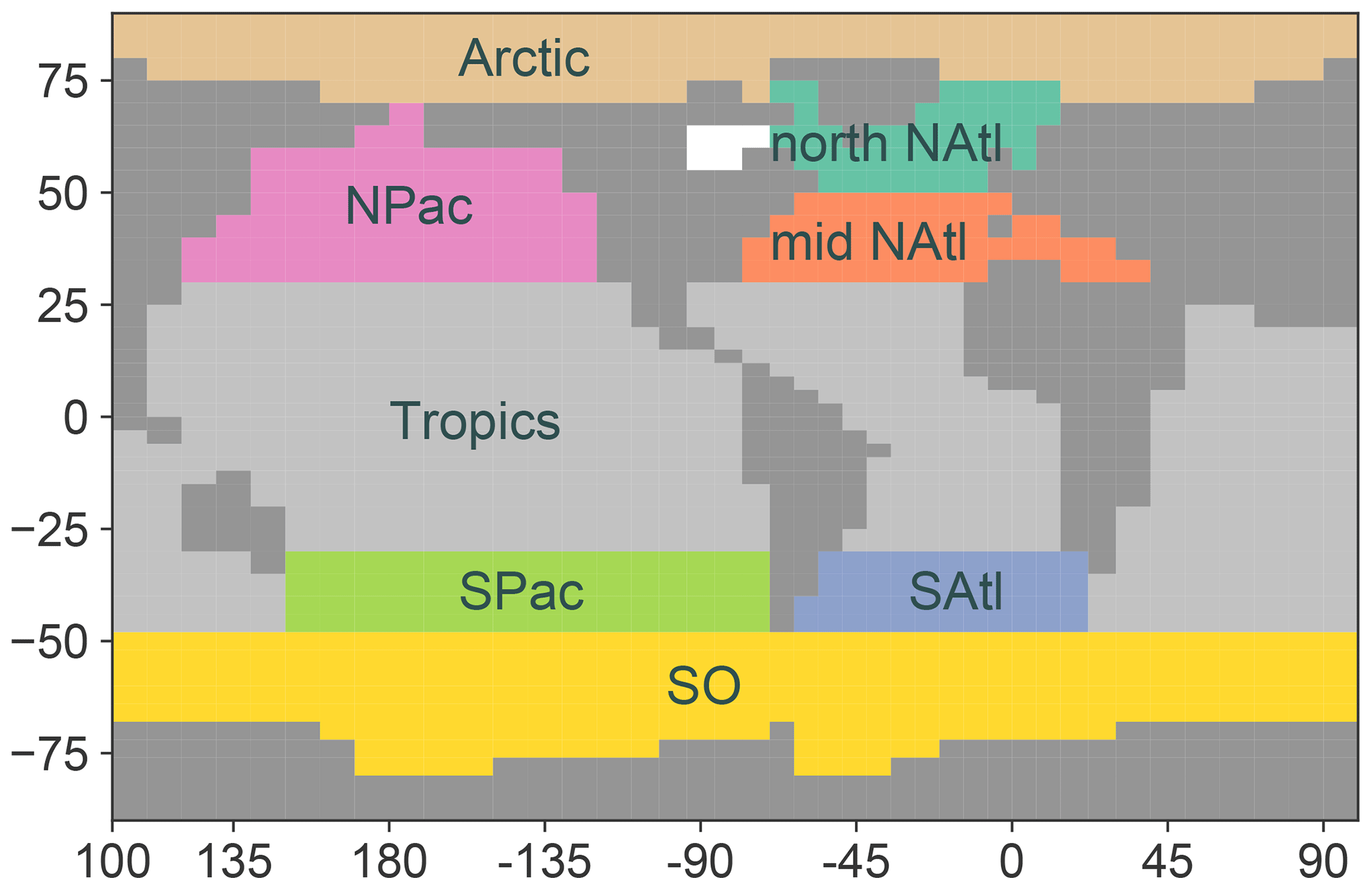
Figure A1Definition of areas as used for regional SST averages on the Bern3D model grid (Fig. 1b, same colours). Simultaneously, these surface areas define where the eight dye tracers originate (Figs. 8, 9 and A3). The dye tracers are named after the water masses they follow: Arctic, North Pacific Intermediate Water (NPIW, in the area NPac), Tropics, South Pacific Intermediate Water (SPIW, in the area SPac), Southern Ocean (SO), North Atlantic Deep Water (NADW, in the area north NAtl), North Atlantic Intermediate Water (NAIW, in the area mid NAtl) and South Atlantic Intermediate Water (SAIW, in the area SAtl). Together they cover the whole ocean surface except the Hudson Bay. The SO dye tracer contains both AABW and AAIW.
A2 Figures regarding standard simulations OcTRA and OcFIX
Figure A3 shows that the water mass shift between SO dye and relatively warmer NADW in Fig. A3a and b explains the observed temperature propagation in the Atlantic (Fig. 4a), which shows a persistent cold anomaly between 2 and 4 km combined with enhanced warming above 2 and below 4 km depth. In this argumentation we used the fact that NADW dye tracer also reaches below 4 km, e.g. occupying 10 %–30 % of the water mass in the South Atlantic at this depth (Fig. 8b). This percentage is larger than expected, because NADW water travelling via the SO back into the deep Atlantic without touching the surface still retains the NADW signature.

Figure A2Hovmöller diagrams of temperature anomalies over depth, decomposed into the effects of (a) changing circulation and (b) changing SST with (c) the total. (a–c) Same as Fig. 4a minus b, Fig. 4b and a (see main text). Values are in centi-Kelvin (1 cK = 10−2 K) and are basin averages of the Atlantic or Pacific (35∘ S–70∘ N) or the Southern Ocean (<35∘ S). Colour levels increase in steps of 5 cK from −20 to 20 cK and in steps of 10 cK otherwise.
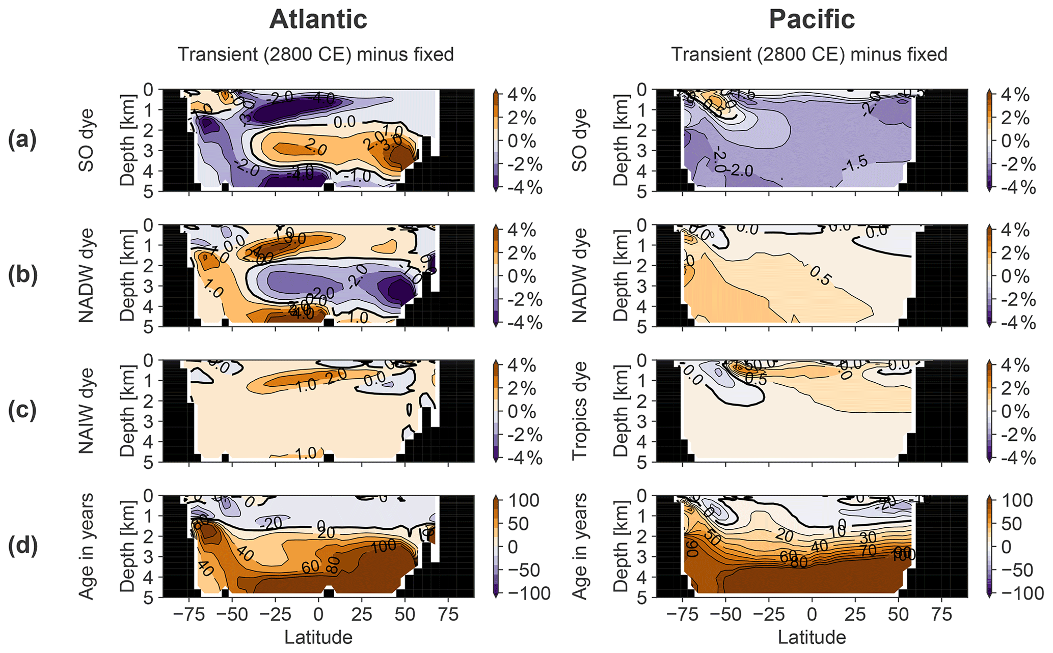
Figure A3Zonally average meridional sections of the Atlantic and Pacific basins, including their Southern Ocean sector. Shown are the anomalies of transient (OcTRA) with respect to fixed (OcFIX) dye tracer for the year 2800 CE (the end of the simulation) of (a) Southern Ocean dye tracer, (b) North Atlantic Deep Water dye tracer, (c) North Atlantic Intermediate Water dye tracer (for Atlantic) and tropics dye tracer (for Pacific), and (d) ideal age. Units for dye are a fraction of initial dye concentration at the surface, in percent.
A3 Figures regarding sensitivity-test simulations
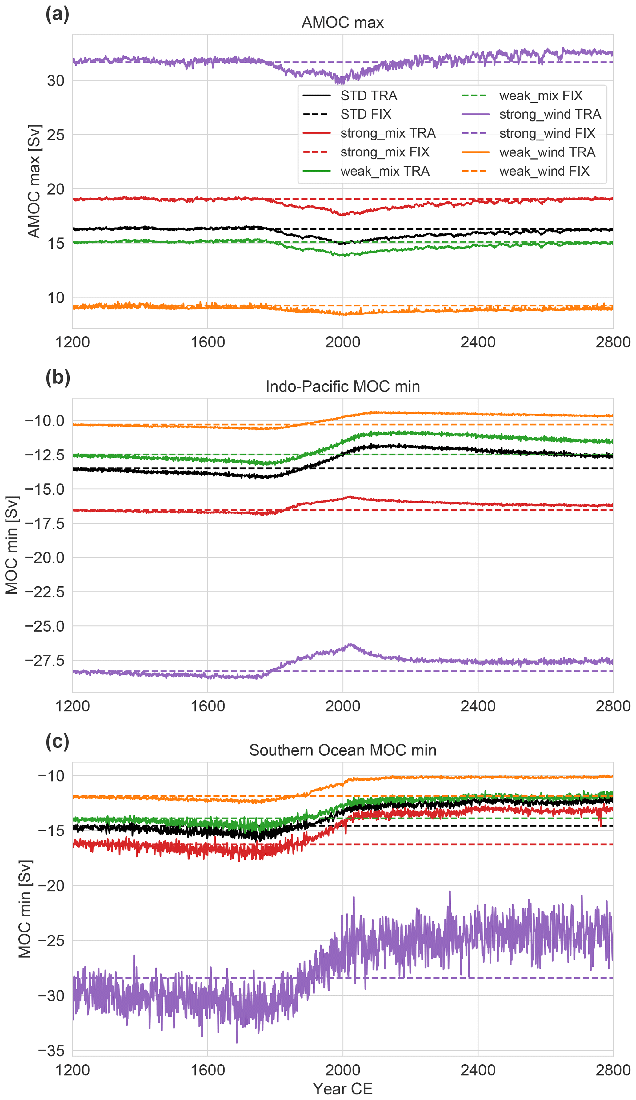
Figure A4For simulations with varying parameters: (a) Atlantic Meridional Overturning Circulation (AMOC) maximum, (b) minimum of the MOC in the combined Pacific and Indian basin (IPMOC) and (c) in the Southern Ocean (SOMOC). Either the wind stress or mixing (i.e. diapycnal diffusivity parameter) is doubled or halved, respectively. TRA stands for transient simulations and FIX for fixed-circulation simulations.

Figure A5Global overturning circulation in a steady state (15-year average) for sensitivity simulations (see Fig. 3c for the standard simulations). The overturning stream function is positive (red) for water rotating clockwise and negative (blue) for water rotating anticlockwise.
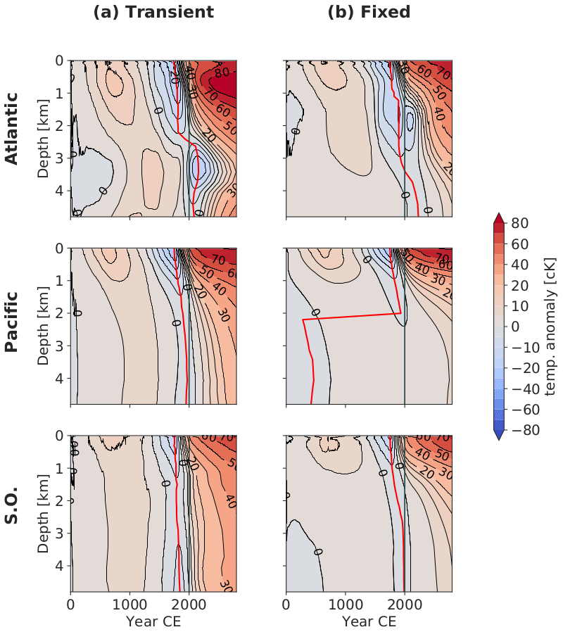
Figure A6Hovmöller diagrams as in Fig. 4a and b (see caption there) but now for simulations (a) OcTRALong (transient) and (b) OcFIXLong (fixed). The minimum temperature anomaly (red line) jumps for the fixed simulation, because no cooling is detected in the Pacific below 2 km. Note the extended time axis from 0 to 2800 CE, because a medieval warm period (MWP) is now included. For OcTRALong and OcFIXLong, SST, SSS and sea ice boundary conditions are read in from a coupled simulation OcAtmTRALong starting at 0 CE with a MWP. For consistency with the later simple evolution, the MWP radiative forcing from 0 to 1200 CE is chosen to be triangular-shaped with a maximum of 0.35 W m−2 at 600 CE (resulting in an SST amplitude comparable to Gebbie and Huybers, 2019). From 1200 CE the forcing is identical to the forcing in Fig. 1a.
This Appendix is related to Sect. 3.4, which discusses the same effects only qualitatively. In this section, we quantitatively estimate the contribution of multiple effects on the deep ocean temperature at 3 km. Instead of a true decomposition, we present a rough estimate of each contribution. This provides more insight into the origin of the leads and lags between TRA and FIX observed at 3 km in the different basins. The results of these calculations are given in Table B3 and interpreted in Sect. B5.
We are about to quantify the following effects:
-
changing SST
-
changing circulation:
- 2a.
water masses
- 2b.
water age.
- 2a.
Throughout this section, variables are only considered at the depth slice of 3.1 km, and within a certain basin, namely the Atlantic, Pacific or Southern Ocean (SO). Typically, variables are computed at steady state, t0=1200 CE, or at a certain time step of interest, , 2000] CE.
Temperature anomalies T=T(t) at 3.1 km depth can be written in terms of water masses i:
where Ti(t) is the typical temperature of a certain water mass and fi(t) is this water mass' fraction between 0 and 1. The sum runs over all water masses i∈ [NADW, NAIW, SAIW, SO, Arctic, NPIW, SPIW, Tropics]. This corresponds to our eight dye tracers, which span the entire ocean surface (Fig. A1). Dropping the time dependence and writing Ti(t) and fi(t) as a sum of their steady state at t0 (subscript 0) and deviation (primed) yields
This decomposition is the main idea of this Appendix. In the following, we reformulate the last three terms one by one, making them more concrete such that we can compute them. The main outcomes are presented in the accompanying Tables; other diagnosed values used can readily be obtained from the available code (python notebook). Results are summarized in Table B3 and their interpretation discussed in Sect. B5.
B1 Effect 1: changing SST
First, we estimate the term corresponding to effect 1, changing SST, at a fixed time of interest t* and depth 3.1 km by
where fi is the fraction of water mass i (between 0 and 1) taken as a basin average at the 3.1 km depth layer and computed at steady state t0. The average corresponds to the average surface temperature anomaly of dye tracer i averaged over the time interval [, ], where amin and amax are the minimum and maximum ideal age at 3.1 km depth occurring in the basin of interest. This is just one of the possible choices that can be made in order to estimate the history of surface temperatures that water mass i has seen at the times of subduction. This choice corresponds to picking a certain time interval in Fig. 1b before the time step of interest t*, which should represent the times of subduction. Here we chose a non-weighted average over all possible times of subduction based on the ideal age tracer a. Note that this is an approximation, because the true age of, for example, the NADW fraction of a certain water parcel is unknown. We only have the ideal age tracer at our disposal, which is the average over the entire probability density function of ages within a water parcel (grid cell) and for example also takes the age of the AABW fraction of this water parcel into account. A second assumption in our approach is taking the average temperature of the surface where a water mass originates as the typical water mass temperature.
Writing out the averaging procedure,
and combining this with the previous gives one final equation for effect 1:
Here, we emphasized that amin and amax are diagnosed at time t0 for effect 1. If either of the times at the integral boundaries occurs before the start of the simulation t0, then the values at t0 are taken, which are representative since the ocean was in steady state before t0. The results of applying Eq. (B1) are shown in Table B1.
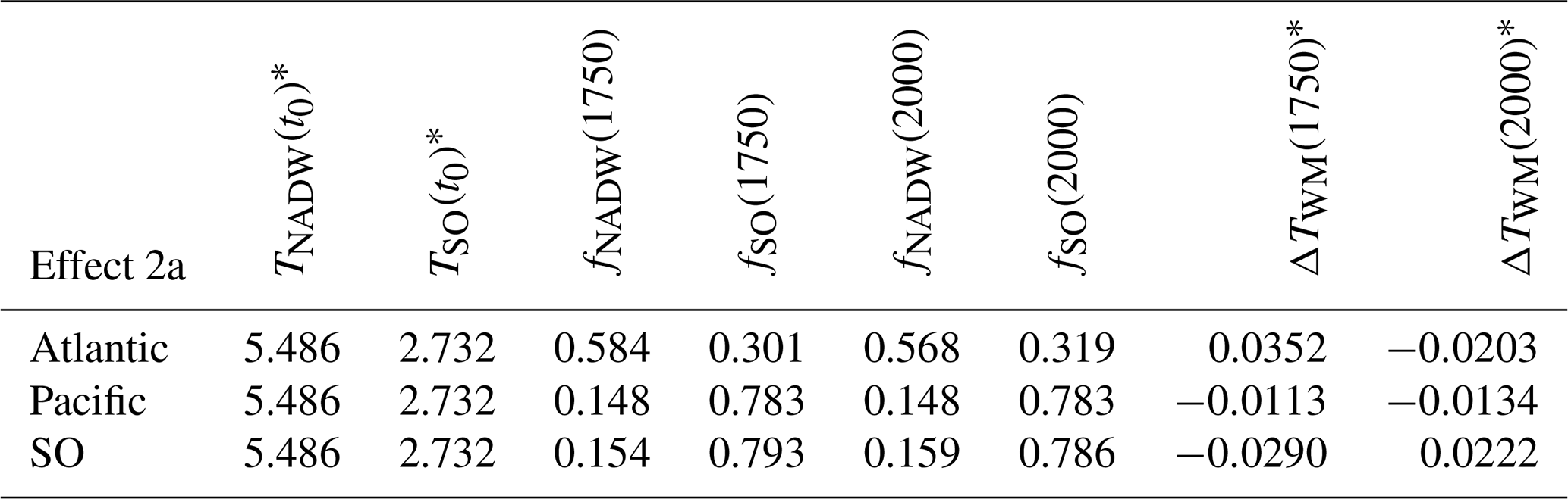
B2 Effect 2a: changing water masses
For effect 1, we multiplied the deviation in water mass temperature with the water mass fraction at steady state. For effect 2a, changing water masses, we now do the opposite: we take the product of the steady state water mass temperature with the deviation of the water mass fraction, again at a time of interest t* and at depth 3.1 km. This gives us the change in temperature at 3.1 km due to water mass changes:
where Ti(t0) is the typical temperature of water mass i at steady state t0, based again on its surface temperature. Note that Ti(t0) relates to ΔTi(t) in Eq. (B1) as . The results are shown in Table B2. The choice of basin does not influence Ti by definition, since the water mass temperature is diagnosed on its specific surface (Fig. A1).
B3 Effect 2b: changing water age
Changing ocean circulation consists of the combined effect of (a) changing water masses (diagnosed by dye tracers) and (b) changing water age (diagnosed by the ideal age tracer). If we adapt the simplified view of two deep water formation end members or pumps, located in the North Atlantic and in the Southern Ocean, then this distinction corresponds to (a) changing the ocean volume filled by each pump (one of the pumps fills more of the ocean volume and the other less) and (b) both pumps increase (decrease) equally in strength such that they turn over faster (slower) within their own overturning cell, which causes a younger (older) water age. It is in principle possible that one of these effects occurs independently without the other, but in reality they typically occur simultaneously and are hard to separate; when an overturning cell increases or decreases in strength, it usually also becomes deeper or shallower. We try this separation nevertheless and estimate the effect of changing water age, representing absolute overturning rate.
Changing water age alters effect 1, changing SST. Since the ages amin and amax shift towards younger (older) values under stronger (weaker) absolute overturning, the ideal ages amin, amax in Eq. (B1) must now be evaluated at t* instead of t0. This gives the effect of water age
where we subtracted effect 1 in order to find only the adjustment due to effect 2b. Since the resulting contribution of water age changes ΔTWA(t*) is relatively small, the diagnosed values of amin(t*), amax(t*) and needed for the calculation are not shown here. The result ΔTWA(t*) is displayed directly in summary Table B3 in cK.
B4 Interaction
The interaction is small, but computed for completeness by combining the deviations of Ti and fi and summing again over all water masses i:
All quantities required for this were already diagnosed and (partly) shown in Tables B1 and B2. The result of Eq. (B4) is directly shown below in the respective column in Table B3.
B5 Final results and interpretation
We summarize the above and compare the contribution of each effect in Table B3, by converting Celsius to centi-Kelvin, by rounding to 2 significant figures with a maximum of 3 decimals and by adding percentages. This table summarizes how much each of the effects, which are discussed qualitatively in Sect. 3.4, quantitatively impacts total deep ocean temperature anomalies, although uncertainties are large (indicated by the “Residual” column; discussion of uncertainty in Sect. B6).
First, the effect of SST history (effect 1) at a fixed 3.1 km depth contributes a cooling in 1750 CE in the deep Atlantic and SO, but no SST-caused cooling reaches the deep Pacific yet. In 2000 CE, the cooling contribution reached the deep Pacific and is still present at this depth in the other basins.
Second, Table B3 confirms the expectation in Sect. 3.4, based on NADW and SO dye tracers, that in 1750 effect 2a (shifting water masses) leads to a warming in the Atlantic and a cooling in the Pacific at 3.1 km. Note that now all eight water masses are taken into account such that a second-order effect is present: relatively more deep water formation water masses (NADW and AABW) relative to other water masses under the LIA forcing, which leads to an additional cooling. In the year 2000, we see a cooling in the Atlantic and Pacific at this depth, again confirming the expectations from dye tracers in Sect. 3.4, whereas the SO warms. Water mass anomalies in 2000 south of 35∘ S (Figs. 8 and 9) show that the SO warming is caused by more NADW-sourced water and less local SO water.
For effect 2b, many values in Table B3 have different signs than expected from the analysis of small ideal age anomalies in Sect. 3.4. We conclude that the values indicated as ≤2 % are indeed not significantly different from zero. Thus, effect 2b has a very small impact at 3.1 km, except in the case of the Atlantic in 2000, where we also observed the largest change in ideal age.
Finally, we compare the relative contributions of effects 1, 2a and 2b. The change in absolute overturning rate, which is estimated via water age, has practically no influence in all cases except the Atlantic in 2000 CE, where the largest overturning anomalies take place. In all other cases, deep ocean temperature anomalies are determined by the interplay of SST and water mass changes. In the Atlantic, SST and water mass changes contribute roughly equally in 1750 but with opposite signs. Therefore, the shifted water masses cause a delay in the arrival of LIA cooling at depth until 1750. In 2000, both water masses and water ages now strongly enhance the amplitude of the cooling, which arrives relatively late. As such, the arrival of the industrial warming is delayed as well. These mechanisms explain the two-century lag observed in the Atlantic and correspond nicely to Fig. 4d, where we see the amplitude of TRA dampened until 1750 but enhanced until 2000 (and further in time). In the Pacific and SO, the contribution of water mass changes generally dominates over SST (except for the SO in 2000). These water mass changes contribute with the same sign as the forcing such that they fasten and enhance the arrival of anomalies at depth. This explains the leads observed in the Pacific and SO and the larger amplitudes in TRA.
B6 Uncertainty
Finally, we make a few closing remarks about uncertainty.
We note that the estimate of effect 1 (changing SST) has a large uncertainty, which explains a substantial amount of the residual column. This is due to the usage of the ideal age tracer as an estimate for the age of a specific water mass, as mentioned above. For example, a water parcel with 75 % NADW with age 200 years and 25 % AABW with age 600 years gives an ideal age of 300 years. In this example, effect 1 is estimated with an NADW age of 300 years and an AABW age of 300 years. This uncertainty of effect 1 can be quantified, because we can also compute effect 1 directly from the output of OcFIX, which gives the “perfect” SST contribution, i.e. exactly as simulated in the Bern3D model. For completion, we list the values of the perfect SST contribution here, in the same order as the rows in Table B3: −0.45, −1.25, −5.07, −6.80, −1.7 and −2.65 cK. Using these perfect values for the SST contribution would result in better residual values: −1.00, −1.36, 0.40, 0.18, −1.63 and 1.15 cK. We did not use these values for consistency reasons, as they do not correspond to the estimates for effect 2b, which is based on effect 1. We conclude that in most cases one-third to two-thirds of the residual is explained by the uncertainty in effect 1.
Effect 2a (changing water masses) is thought to be well-known, since it does not use the ideal age tracer to estimate water mass age. The uncertainty in effect 1 propagates in effect 2b (changing water ages), since it is based on effect 1. As an uncertainty estimate for effect 2b, we take the percentage uncertainty in the SST contribution quantified above and take the same percentage as uncertainty for effect 2b. This gives an uncertainty of roughly 200 % to 300 % for most basins and most time steps. Note that this uncertainty is not symmetric, since the SST estimate is generally too small, and thus we also expect effect 2b to be too small rather than too large (in absolute values). Scaling the percentage contribution of effect 2b (Table B3) by a factor of 2 or 3 typically changes values of 2 % to a maximum of 6 %, and hence they are still very small. We conclude that the uncertainty in effect 2b is large, but this does not change our main message of effect 2b being small in all cases, except perhaps in the Atlantic in 2000 CE.
Table B1Computing effect 1, changing SST. The first six columns containing data present a subset of the diagnosed values needed for the computation: as an example, only water masses NADW and SO and only are shown. The two rightmost columns show the result of effect 1 by using Eq. (B1), where all eight water masses were taken into account.

a Ages amin and amax are in years. b Averaged temperatures and results ΔTSST are in ∘C.
Table B2Computing effect 2a, changing water masses. The first six columns containing data present a subset of the diagnosed values needed for the computation: as an example, only water masses NADW and SO are shown. In addition, fi(t0) from Table B1 are used. The two rightmost columns show the result of effect 2a by using Eq. (B2), where all eight water masses were taken into account.
* Temperatures are in ∘C.
Table B3Summary of quantification of how different effects act on the deep ocean temperature at 3.1 km, per basin and at times of interest 1750 CE and 2000 CE. All values are temperature anomalies with respect to 1200 CE in centi-Kelvin (cK). Percentages are added in parentheses, where the residual is excluded; i.e. 100 % corresponds to the sum of effects 1, 2a, 2b and their interaction. For the percentage, the absolute value of each contribution is taken.
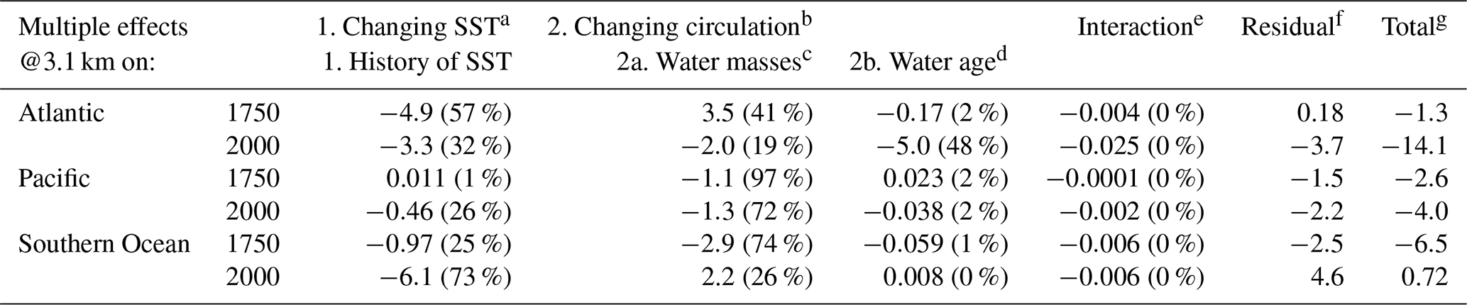
a Results are taken over from Table B1 and converted to cK. b Changing circulation consists of the – not necessarily independent – subeffects 2a and 2b. c Results are taken over from Table B2 and converted to cK. d The water-age contribution follows from Eq. (B3). e The interaction is the cross term of deviations between effect 1 and 2a and follows from Eq. (B4). f The residual equals the total minus effects 1, 2a, 2b and the interaction. It represents unaccounted effects and uncertainties in the calculations. g The total of all effects is given by the model output of OcTRA, which is averaged at 3.1 km within the basin of interest.
The Bern3D model is closed-source, but the output of all model simulations used in this study is available in netCDF format (Scheen et al., 2020). The analysis code that was used to make the figures and to perform the calculations in Appendix B is available as a well-documented python notebook (Scheen, 2020). In the case of questions or suspected bugs, please contact Jeemijn Scheen. For Fig. 11c, data were used from https://www2.whoi.edu/staff/ggebbie/ (last access: 8 September 2020) (Gebbie and Huybers, 2020).
JS carried out the numerical simulations, implementation and analysis. TFS conceived the original idea and supervised the project. JS lead the writing of the paper. Both authors contributed to the interpretation of the results.
The authors declare that they have no conflict of interest.
We thank Woon Mi Kim and Angelique Hameau for providing the sea surface salinity output of CESM1.0.1 during the past millennium. We gratefully acknowledge Thomas L. Frölicher for helpful comments on an earlier version of the manuscript and two anonymous reviewers for their constructive feedback, which improved the paper. We thank Geoffrey Gebbie for providing the data for Fig. 11c and details on their analysis.
This research has been supported by the Swiss National Science Foundation (grant no. SNF 200020_172745).
This paper was edited by Gerrit Lohmann and reviewed by two anonymous referees.
Banks, H. T. and Gregory, J. M.: Mechanisms of ocean heat uptake in a coupled climate model and the implications for tracer based predictions of ocean heat uptake, Geophys. Res. Lett., 33, L07608, https://doi.org/10.1029/2005GL025352, 2006. a, b
Brönnimann, S., Franke, J., Nussbaumer, S., Zumbühl, H., Steiner, D., Trachsel, M., Hegerl, G., Schurer, A., Worni, M., Malik, A., Flückiger, J., and Raible, C.: Last phase of the Little Ice Age forced by volcanic eruptions, Nat. Geosci., 12, 650–656, https://doi.org/10.1038/s41561-019-0402-y, 2019. a
Collins, M., Sutherland, M., Bouwer, L., Cheong, S.-M., Frölicher, T., Jacot Des Combes, H., Koll Roxy, M., Losada, I., McInnes, K., Ratter, B., Rivera-Arriaga, E., Susanto, R. D., Swingedouw, D., and Tibig, L.: Extremes, Abrupt Changes and Managing Risk, in: IPCC Special Report on the Ocean and Cryosphere in a Changing Climate, edited by: Pörtner, H.-O., Roberts, D. C., Masson-Delmotte, V., Zhai, P., Tignor, M., Poloczanska, E., Mintenbeck, K., Alegría, A., Nicolai, M., Okem, A., Petzold, J., Rama, B., and Weyer, N., available at: https://www.ipcc.ch/srocc/chapter/chapter-6/ (last access: 20 August 2020), 2019. a
Edwards, N. R., Willmott, A. J., and Killworth, P. D.: On the Role of Topography and Wind Stress on the Stability of the Thermohaline Circulation, J. Phys. Oceanogr., 28, 756–778, https://doi.org/10.1175/1520-0485(1998)028<0756:OTROTA>2.0.CO;2, 1998. a
Emile-Geay, J., McKay, N., Kaufman, D., Von Gunten, L., Wang, J., Anchukaitis, K., Abram, N., Addison, J., Curran, M., Evans, M., Henley, B., Hao, Z., Martrat, B., McGregor, H., Neukom, R., Pederson, G., Stenni, B., Thirumalai, K., Werner, J., and Zinke, J.: A global multiproxy database for temperature reconstructions of the Common Era, Scient. Data, 4, 170088, https://doi.org/10.1038/sdata.2017.88, 2017. a
England, M. H.: The Age of Water and Ventilation Timescales in a Global Ocean Model, J. Phys. Oceanogr., 25, 2756–2777, https://doi.org/10.1175/1520-0485(1995)025<2756:TAOWAV>2.0.CO;2, 1995. a
Garuba, O. A. and Klinger, B. A.: Ocean Heat Uptake and Interbasin Transport of the Passive and Redistributive Components of Surface Heating, J. Climate, 29, 7507–7527, https://doi.org/10.1175/JCLI-D-16-0138.1, 2016. a, b, c
Gebbie, G. and Huybers, P.: The Mean Age of Ocean Waters Inferred from Radiocarbon Observations: Sensitivity to Surface Sources and Accounting for Mixing Histories, J. Phys. Oceanogr., 42, 291–305, https://doi.org/10.1175/JPO-D-11-043.1, 2012. a, b
Gebbie, G. and Huybers, P.: The Little Ice Age and 20th-century deep Pacific cooling, Science, 363, 70–74, https://doi.org/10.1126/science.aar8413, 2019. a, b, c, d, e, f, g, h, i, j, k
Gebbie, G. and Huybers, P.: Data behind Fig. 2 of Gebbie & Huybers 2019, available at: https://www2.whoi.edu/staff/ggebbie/, last access: 8 September 2020. a
Hall, T. and Haine, T.: On Ocean Transport Diagnostics: The Idealized Age Tracer and the Age Spectrum, J. Phys. Oceanogr., 32, 1987–1991, https://doi.org/10.1175/1520-0485(2002)032<1987:OOTDTI>2.0.CO;2, 2002. a
Mann, M., Bradley, R., and Hughes, M.: Global-Scale Temperature Patterns and Climate Forcing Over the Past Six Centuries, Nature, 392, 779–787, https://doi.org/10.1038/33859, 1998. a
Mann, M. E., Zhang, Z., Rutherford, S., Bradley, R. S., Hughes, M. K., Shindell, D., Ammann, C., Faluvegi, G., and Ni, F.: Global Signatures and Dynamical Origins of the Little Ice Age and Medieval Climate Anomaly, Science, 326, 1256–1260, https://doi.org/10.1126/science.1177303, 2009. a
Marshall, J., Scott, J., Armour, K., Campin, J.-M., Kelley, M., and Romanou, A.: The ocean's role in the transient response of climate to abrupt greenhouse gas forcing, Clim. Dynam., 44, 2287–2299, https://doi.org/10.1007/s00382-014-2308-0, 2015. a, b
Masson-Delmotte, V., Schulz, M., Abe-Ouchi, A., Beer, J., Ganopolski, A., González Rouco, J. F., Jansen, E., Lambeck, K., Luterbacher, J., Naish, T., Osborn, T., Otto-Bliesner, B., Quinn, T., Ramesh, R., Rojas, M., Shao, X., and Timmermann, A.: Chapter 5: Information from Paleoclimate Archives, in: Climate Change 2013: The Physical Science Basis, Contribution of Working Group I to the Fifth Assessment Report of the Intergovernmental Panel on Climate Change, edited by: Stocker, T. F., Qin, D., Plattner, G.-K., Tignor, M., Allen, S. K., Boschung, J., Nauels, A., Xia, Y., Bex, V., and Midgley, P. M., Cambridge University Press, Cambridge, 383–464, available at: https://archive.ipcc.ch/pdf/assessment-report/ar5/wg1/WG1AR5_Chapter05_FINAL.pdf (last access: 15 May 2020), 2013. a
McGregor, H. V., Evans, M. N., Goosse, H., Leduc, G., Martrat, B., Addison, J. A., Mortyn, P. G., Oppo, D. W., Seidenkrantz, M.-S., Sicre, M.-A., Phipps, S. J., Selvaraj, K., Thirumalai, K., Filipsson, H. L., and Ersek, V.: Robust global ocean cooling trend for the pre-industrial Common Era, Nat. Geosci., 8, 671–677, https://doi.org/10.1038/ngeo2510, 2015. a
Moffa-Sánchez, P., Moreno-Chamarro, E., Reynolds, D. J., Ortega, P., Cunningham, L., Swingedouw, D., Amrhein, D. E., Halfar, J., Jonkers, L., Jungclaus, J. H., Perner, K., Wanamaker, A., and Yeager, S.: Variability in the Northern North Atlantic and Arctic Oceans Across the Last Two Millennia: A Review, Paleoceanogr. Paleocl., 34, 1399–1436, https://doi.org/10.1029/2018PA003508, 2019. a
Müller, S. A., Joos, F., Edwards, N. R., and Stocker, T. F.: Water Mass Distribution and Ventilation Time Scales in a Cost-Efficient, Three-Dimensional Ocean Model, J. Climate, 19, 5479–5499, https://doi.org/10.1175/JCLI3911.1, 2006. a
Neukom, R., Steiger, N., Gómez-Navarro, J. J., Wang, J., and Werner, J. P.: No evidence for globally coherent warm and cold periods over the preindustrial Common Era, Nature, 571, 550–554, https://doi.org/10.1038/s41586-019-1401-2, 2019. a, b
PAGES 2k Consortium: Continental-scale temperature variability during the past two millennia, Nat. Geosci., 6, 339–346, https://doi.org/10.1038/ngeo1834, 2013. a, b, c, d
Rayner, N. A., Parker, D. E., Horton, E. B., Folland, C. K., Alexander, L. V., Rowell, D. P., Kent, E. C., and Kaplan, A.: Global analyses of sea surface temperature, sea ice, and night marine air temperature since the late nineteenth century, J. Geophys. Res.-Atmos., 108, 4407, https://doi.org/10.1029/2002JD002670, 2003. a, b
Ritz, S. P., Stocker, T. F., and Joos, F.: A Coupled Dynamical Ocean–Energy Balance Atmosphere Model for Paleoclimate Studies, J. Climate, 24, 349–375, https://doi.org/10.1175/2010JCLI3351.1, 2011. a, b
Roth, R., Ritz, S. P., and Joos, F.: Burial-nutrient feedbacks amplify the sensitivity of atmospheric carbon dioxide to changes in organic matter remineralisation, Earth Syst. Dynam., 5, 321–343, https://doi.org/10.5194/esd-5-321-2014, 2014. a, b
Scheen, J.: Effect of changing ocean circulation on deep ocean temperature in the last millennium: code, Zenodo, https://doi.org/10.5281/zenodo.4022947, 2020. a
Scheen, J., Gebbie, G., and Stocker, T. F.: Effect of changing ocean circulation on deep ocean temperature in the last millennium: simulation output data, Zenodo, https://doi.org/10.5281/zenodo.4022927, 2020. a
Steiger, N., Smerdon, J., Cook, E., and Cook, B.: A reconstruction of global hydroclimate and dynamical variables over the Common Era, Scient. Data, 5, 180086, https://doi.org/10.1038/sdata.2018.86, 2018. a
Winton, M., Griffies, S. M., Samuels, B. L., Sarmiento, J. L., and Frölicher, T. L.: Connecting Changing Ocean Circulation with Changing Climate, J. Climate, 26, 2268–2278, https://doi.org/10.1175/JCLI-D-12-00296.1, 2013. a, b, c, d, e, f, g, h, i, j, k, l, m
Xie, P. and Vallis, G.: The passive and active nature of ocean heat uptake in idealized climate change experiments, Clim. Dynam., 38, 667–684, https://doi.org/10.1007/s00382-011-1063-8, 2011. a, b, c, d
- Abstract
- Introduction
- Modelling framework
- Results and discussion
- Sensitivity of leads and lags
- Comparison to Gebbie and Huybers (2019)
- Conclusions and outlook
- Appendix A: Figures
- Appendix B: Quantification of effects causing leads and lags at 3 km
- Code and data availability
- Author contributions
- Competing interests
- Acknowledgements
- Financial support
- Review statement
- References