the Creative Commons Attribution 4.0 License.
the Creative Commons Attribution 4.0 License.
 | 16 Jul 2020
Climate change in a conceptual atmosphere–phytoplankton model
Rudolf Dániel Prokaj
István Scheuring
Tamás Tél
We develop a conceptual coupled atmosphere–phytoplankton model by combining the Lorenz'84 general circulation model and the logistic population growth model under the condition of a climate change due to a linear time dependence of the strength of anthropogenic atmospheric forcing. The following types of couplings are taken into account: (a) the temperature modifies the total biomass of phytoplankton via the carrying capacity; (b) the extraction of carbon dioxide by phytoplankton slows down the speed of climate change; (c) the strength of mixing/turbulence in the oceanic mixing layer is in correlation with phytoplankton productivity. We carry out an ensemble approach (in the spirit of the theory of snapshot attractors) and concentrate on the trends of the average phytoplankton concentration and average temperature contrast between the pole and Equator, forcing the atmospheric dynamics. The effect of turbulence is found to have the strongest influence on these trends. Our results show that when mixing has sufficiently strong coupling to production, mixing is able to force the typical phytoplankton concentration to always decay globally in time and the temperature contrast to decrease faster than what follows from direct anthropogenic influences. Simple relations found for the trends without this coupling do, however, remain valid; just the coefficients become dependent on the strength of coupling with oceanic mixing. In particular, the phytoplankton concentration and its coupling to climate are found to modify the trend of global warming and are able to make it stronger than what it would be without biomass.
- Article
(2887 KB) - Full-text XML
-
Supplement
(239 KB) - BibTeX
- EndNote


Large-scale general circulation models typically take into account the interaction of the atmosphere with land vegetation and marine biomass production in the form of a huge number of parametrized processes (see, e.g., Marinov et al., 2010; Zhong et al., 2011; Mongwe et al., 2018; Wilson et al., 2018). A basic understanding of such coupling is, however, easier to obtain in low-order conceptual models, where even analytic results may be available. Probably the most important component that needs to be included in such conceptual models is the phytoplankton content of the ocean.
Oceans are the major sink for the atmospheric CO2 (Hader et al., 2014; Li et al., 2012). CO2 is either stored as dissolved inorganic carbon or transferred to the underlying sediment by biological carbon pump. The motor of the biological pump is phytoplankton, which is one of the major components of the global carbon cycle, hence influencing decisively atmospheric CO2 (Hutchins and Fu, 2017; Sanders et al., 2014; Turner, 2005; Falkowski et al., 2000). Besides, phytoplankton is responsible for nearly half of the total primary production on Earth (Basu and Mackey, 2018). Consequently, it is extremely important to understand the interaction of phytoplankton in oceans with effects contributing to global climate change. However, the task is very challenging; change in atmospheric CO2 level can have opposite impacts on processes influencing the phytoplankton and the intensity of the biological carbon pump. Increased atmospheric CO2 level increases ocean temperature, decreases pH, increases water stratification, and influences general oceanic circulation. These can all modify the net productivity and the composition of phytoplankton and can have either a positive or negative net effect on the biological carbon pump (Basu and Mackey, 2018, and references therein).
In spite of the current trend to include biogeochemistry in climate models (see, e.g., Schlunegger et al., 2019), a basic understanding of such processes is still limited. It is still under debate whether net primary production is increasing or decreasing in coupled carbon–climate models as a consequence of warming-induced production increase and stronger nutrient limitations induced by increased stratification (Laufkötter et al., 2015). The situation appears to be similar to the understanding of thermal or fluid dynamical concepts decades ago. The study of, e.g., the energy balance (Ghil, 1976) or the thermohaline circulation (Stommel, 1961) started with elementary conceptual models which later evolved into more complex ones and are by now decisive components of cutting-edge climate models. We therefore propose here to study a conceptual atmosphere–phytoplankton model where emphasis is on a proper choice of couplings (feedbacks). Thus, in our model, an increase in the global temperature affects the global primary production of ocean. As we emphasize above, phytoplankton plays significant role in the global CO2 balance (De La Rocha and Passow, 2014; Falkowski, 2014; Guidi et al., 2016); hence our aim is to take an elementary description of phytoplankton dynamics coupled to an elementary model of the atmosphere. The direct effect of increased CO2 concentration on phytoplankton dynamics can be stimulating or inhibiting; we study both scenarios. As atmospheric model, we use Lorenz's elementary global circulation model (Lorenz, 1984), which was extended to mimic climate change (Drótos et al., 2015). The global phytoplankton concentration is represented by a simple logistic model in which the carrying capacity is coupled with the CO2 content (direct effect) depending also on the concentration itself and on the wind energy influencing the oceanic mixing layer (indirect effect of climate change).
An appropriate treatment of even elementary models describing climate change is not obvious, since basic parameters change with time, and, therefore, traditional long-time averages cannot be used to define (in the sense of any statistical quantifiers) a state of the climate. An emerging new view, already embraced by Drótos et al. (2015), follows a different route to obtain information on instantaneous statistical quantifiers (e.g., expected, average properties) of the climate. Since our information on the actual state of the climate is incomplete, one imagines an ensemble of parallel Earth systems carrying parallel climate realizations subjected to the same set of physical laws, boundary conditions, and external forcing but with different initial conditions. Then the chaotic or turbulence-like properties of the climate dynamics allows for distinct climate realizations (for a review, see Tél et al., 2019). These realizations, however, cannot be arbitrary, since only those that are compatible with physical laws and the given forcing are permitted. The ensemble of realizations defines a probability distribution of all the relevant variables at any instant of time from which one can obtain expected ensemble average properties of the climate (for more details, and mathematical aspects, see Sect. 5).
It is therefore natural to use the ensemble view in our conceptual biogeochemistry model, too. The ensemble approach in it corresponds to generating parallel atmosphere–phytoplankton realizations from different initial conditions. In our model, the number of variables is four; hence the snapshot attractor in the full state space is difficult to visualize. We therefore concentrate on ensemble averages, and the internal variability will be expressed in terms of variances. We include, in a simple heuristic form, important feedbacks in the model: (a) the change in the atmospheric temperature that modifies phytoplankton concentration; (b) the extraction of CO2 by phytoplankton; and (c) wind energy that enhances the strength of turbulence in the oceanic mixing layer, which increases the phytoplankton production (Estrada and Berdalet, 1997; Peters and Marrasé, 2000; Jäger et al., 2010).
The paper is organized as follows. In Sect. 2 we describe the model and define the relevant coupling parameters. Without mixing, exact relations can be derived. The most important of these are summarized in Sect. 3, while details of the calculations are relegated to Sect. S1 in the Supplement . In the presence of mixing, numerical simulations are carried out in the spirit of snapshot attractors. The results are summarized in Sect. 4 where one learns that the extraction effect of CO2 has the least influence on the general behavior in the presence of mixing. The feedback of the temperature contrast on the phytoplankton concentration has important consequences, but these are suppressed by a sufficiently strong mixing, which converts the typical phytoplankton concentration to always decay in time, and surprisingly, the typical temperature contrast is found to decrease faster than that solely by direct anthropogenic effects. Planar sections of the 4-dimensional snapshot attractor underlying the dynamics are presented in Sect. 5, and our conclusions are drawn in Sect. 6. Additional figures are presented in Sect. S2 in the Supplement . A list of variables and parameters is given in Sect. S3, while Sect. S4 contains a sample of the C code applied during numerical simulations.
The physical content of Lorenz's atmospheric circulation model for the midlatitudes (Lorenz, 1984, 1990) on one hemisphere is the following. The main forcing is the temperature difference Te−Tp between the Equator and the pole. This is proportional to model variable F influencing most directly the wind speed of the Westerlies represented by x. As an effect of baroclinic instability, cyclonic activity facilitates poleward heat transport, two modes of which are represented by y and z. The model reads as follows:
For the parameter setting we take the common choice: , b=4, and G=1. The equations appear in a dimensionless form with the time unit corresponding to 5 d.
By using time-dependent forcing, F(t), as Drótos et al. (2015), we also model the contribution of the varying CO2 content in association with the greenhouse effect. Besides the variation in CO2 due to effects appearing in F(t), the extraction of CO2 by phytoplankton is also included into our model. The CO2 content stored in marine ecosystems or buried in the seabed is correlated with primary production (Falkowski et al., 1998, 2003). Thus, as discussed in the Introduction, modeling the interaction of phytoplankton and atmospheric dynamics is a good proxy for the studying marine ecosystem interaction with atmospheric dynamics. Hence, we couple the Lorenzian atmospheric dynamics to that of the photosynthesizing oceanic biomass, assumed to be dominated by phytoplankton of concentration c(t). The temperature contrast parameter thus also depends on the global phytoplankton concentration c: , with a form to be given below.
Spatial inhomogeneities in nutrient and consequently phytoplankton content due to, e.g., oceanic eddies and upwellings are known to play an important local role in nature. However, a global atmospheric model like Eq. (1) can adequately be coupled only to a global phytoplankton dynamics model. Therefore, the concentration itself is assumed in this simple setup to follow a logistic population growth
Carrying capacity K is taken to depend on the average temperature of the hemisphere or, equivalently, on the temperature contrast F. As a consequence, K depends on time also via the concentration c: . We shall see that an important oceanic effect, that of the turbulence in the mixing layer, can be incorporated into carrying capacity K, although only on a global scale. Parameter r sets the growth rate of the phytoplankton. If, e.g., r=1, the phytoplankton characteristic time is d, as that of the atmosphere. This latter choice will be kept throughout the paper. The assumption of Eq. (2) for the global phytoplankton dynamics tacitly implies that phytoplankton biomass determines the total biomass of the oceans and also that no catastrophic events (no mass extinction or invasion of species) can take place in this model.
A basic feature of the observed climate change on Earth is that the polar temperature Tp(t) increases, while the equatorial one Te remains practically constant (Serezze and Francis, 2006; Blunden and Arndt, 2013). We can thus write in suitable units the temperature contrast parameter as . The mean temperature in these units is then . We are interested in dominant, leading-order effects and assume therefore the carrying capacity to be coupled linearly by a small coupling constant to the mean temperature relative to some reference state of mean temperature Tr, in which the temperature contrast parameter is . The temperature difference T−Tr is then . We therefore write
where Kr is the carrying capacity in the reference state characterized by Fr. Coefficient α represents coupling (a) between the carrying capacity K and climate change, represented by F, and shall be called the enrichment parameter; see Fig. 1 where the full set of feedbacks considered in the model is schematically presented. This coupling may be either positive or negative. For example, increased CO2 level enhances the efficiency of photosynthesis (α>0); however, acidification because of increased CO2 levels depresses respiration (α<0) (Reid et al., 2009; Mackey et al., 2015). Similarly, increased water temperature can have both a positive and negative effect on phytoplankton biomass in different regions of Earth (Chust et al., 2014; Roberts et al., 2017). We shall, therefore, allow for both positive and negative values of α with small.
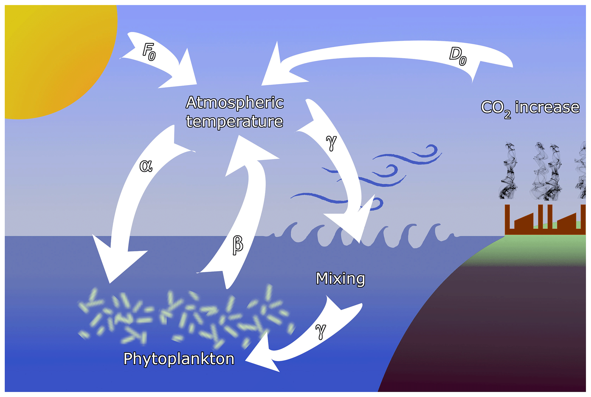
Figure 1Sketch of the feedbacks considered in the model. Temperature contrast F0 between the pole and the Equator, containing also seasonal variability, is augmented by anthropogenic effects D0. The main interactions are (α) the enrichment effect of atmospheric temperature on phytoplankton, (β) the extraction of CO2 by phytoplankton, and (γ) oceanic mixing, driven by atmospheric dynamics, affecting phytoplankton productivity.
Phytoplankton dynamics influences the temperature contrast. If concentration c increases, the temperature contrast F increases, too, because the biomass extracts more CO2. In leading order, we therefore express the concentration-dependent temperature contrast parameter as a linear function of the concentration:
with a small β>0, where cr is the phytoplankton concentration in the reference state. Coefficient β represents coupling (b) due to the extraction of CO2 by phytoplankton, and we therefore call β the extraction parameter (see Fig. 1). The second term, F0(t), represents the primary external forcing due to the CO2 content of anthropogenic origin. The increase in both F0 and (c(t)−cr) leads to an increase in the temperature contrast F(t). With this form of F the carrying capacity (3) is
Without a restriction of generality, we can choose the reference carrying capacity to be Kr=1, implying a reference concentration cr=1. This choice only rescales parameters α and β in Eqs. (3) and (4), respectively.
Starting from negative times, we assume the Earth system to be in climatic and population dynamical equilibrium up to time t=0. This state, chosen as the reference state, is characterized by a time-independent mean temperature Tr, concentration cr=Kr, and F0(t)=Fr. At time zero, climate change sets in expressed by a linear decrease in the primary temperature contrast as follows:
expressing direct anthropogenic effects, with a decrease parameter for t>0 (Drótos et al., 2015). Since 1 year corresponds to 73 time units (365 d), 1 year = 73, this form expresses that the temperature contrast decreases by 2 units over 100 years. We shall take Fr=9.5, with which the temperature contrast would go down, after a climate change period of 150 years and without any change in the biomass concentration, to 6.5. We stop the climate change scenario in year 150 because the model from Eq. (1) loses its global chaotic property, which is a prerequisite even for a minimal climate model, for small F.
With this scenario in Eq. (6) of the anthropogenic influence, the carrying capacity K(t) is, in rescaled units,
where D0=0 for t≤0 and for t>0.
We can model seasonality, too, as Lorenz also did (Lorenz, 1990), by augmenting Eq. (6) with a periodic term as follows:
His choice was A=2 with , which we shall adopt. Our climate change starts with year 0, and this year begins at the time instant t=0. Note that this time instant belongs to an autumnal equinox according to Eq. (8), and, furthermore, Fr−D0t can be considered as the annual mean temperature contrast. Any time t mod 73=0 coincides with other autumnal equinoxes, and results will be presented on this day of the year throughout the paper.
Up to this point, the atmospheric variables have not entered the concentration dynamics. Without the linear and constant terms (representing dissipation and forcing, respectively), Eq. (1) would conserve the total kinetic energy
of the atmosphere. From the point of view of the biomass, it is natural to assume that the activity of the atmosphere influences the ocean dynamics within its uppermost mixing layer (Sverdrup, 1953; Whitt et al., 2017), in particular, the strength of turbulence, and hence the depth of mixing layer. Note that component represents the contribution of zonal winds to the total atmospheric energy, while represents wind energy stemming from cyclonic activity. The depth of the mixing layer and, consequently, the carrying capacity are assumed to increase linearly with E in our model, with a small coupling constant. The most general form of the carrying capacity K is thus
Here is the strength of a weak coupling (c) due to oceanic mixing what we call the (oceanic) mixing parameter. This provides a feedback between the phytoplankton dynamics and the climatic variables (see Fig. 1).
Without mixing (γ=0), Eq. (2) can be solved by a simple ansatz of c(t), irrespective of the atmospheric dynamics. This leads to analytic results concerning some properties of the model, which are summarized in Sect. S1. As an example, we give here two simple relations which help one to understand the general tendencies of the system. Equation (2) with (9) is shown for γ=0 to possess linear behavior for long times, inherited from the temperature contrast of anthropogenic origin as follows:
Naively, one expects that an increased CO2 level (smaller F in Eq. 1) leads to a higher carrying capacity and concentration of the phytoplankton, and a slower decrease of the temperature contrast, i.e., S (D) should increase (decrease) with the enrichment parameter. However, only calculating the precise dependence can reveal whether these trends are important or hardly discernible. The linear coefficient slope S in the phytoplankton concentration's time dependence is found to be
The approximate equality reflects that the product α⋅β is quadratically small, since both the enrichment parameter α and the extraction parameter β are small quantities. Hence the leading-order behavior in α is linear. This relation shows that for a positive (negative) coupling, α the phytoplankton concentration increases (decreases) proportionally with the enrichment parameter α and with the slope D0 of the anthropogenic temperature contrast.
The linear coefficient in the temperature contrast is
The approximate equality provides, again, the leading-order behavior in α. The relation indicates that in the case of a positive enrichment parameter α, the phytoplankton dynamics weakens the climate change, weakens the trend from D0 to D in the temperature contrast, as expected. Quite surprisingly, however, the effect is rather weak since α⋅β is quadratically small. Relations (11) and (12) also suggest that the role of (a weak) extraction coupling is not essential; the leading behavior in S is independent of β. Its effect is weak also in D. This quantity coincides with the anthropogenic slope D0 for β=0 (as also follows from Eq. 4); it deviates from D0 very little otherwise.
It is worth noting that relations (11) and (12) remain valid for the time-averaged trends in the presence of a seasonal periodicity, as also shown in Sect. S1. Relations (11) and (12) are independent of initial conditions; they represent the snapshot attractor of the problem projected on variable c. This attractor is fixed-point-like but changes in time (moves uniformly or with an oscillation superimposed when seasonality is taken into account). There is, however, no internal variability in the concentration variable c, although an extended, fractal snapshot attractor underlies the atmospheric variables exactly as in the model of Drótos et al. (2015), where phytoplankton dynamics was not taken into account.
In the interesting case of non-negligible mixing, no analytic result can be obtained. This implies a nontrivial biomass dynamics for γ>0, a dynamics exhibiting internal variability in variable c, too. To explore this regime, we carried out a sequence of numerical simulations of the full four-variable dynamics. The following parameters are kept fixed (as indicated in the previous section): r=1, , Fr=9.5, A=2, and . We vary α, β, and γ. Equations (1) and (2) with (4), (8), and (9) are solved with the classical fourth-order Runge–Kutta method with a fixed timestep years.
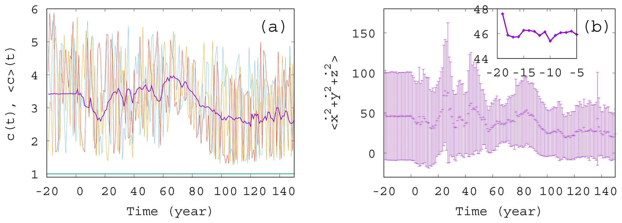
Figure 2Ensemble properties before (t<0) and after (t>0) the onset of climate change. (a) Phytoplankton concentration c as a function of time for three random initial conditions in different colors for α=0.05, β=0.1, and γ=0.1. The purple line is the ensemble average for 50 000 trajectories started with random initial positions in the range ; ; and at year −20. The green line (close to c=1) shows the expected phytoplankton concentration without any mixing (γ=0) as predicted by Eq. (10). (The increase for t>0 is so weak that one hardly recognizes it on this graph.) (b) Time dependence of the ensemble average (dark violet “+” marks) of the total atmospheric kinetic energy for the same ensemble as the one used for c in panel (a). Violet bars indicate the standard deviation. The inset shows the blowup of the initial part of the average in panel (b).
To start with, Fig. 2a shows a few individual concentration realizations (colored lines) c(t) for a mixing parameter γ=0.1 (α=0.05 and β=0.1), along with the ensemble average of 50 000 realizations initiated at years (purple line). Here and in what follows angled brackets will always denote averages taken with respect to our ensemble at a given time instant, t. The individual cases are all rather different. For t<0 there is no climate change, but nevertheless, the individual time series c(t) exhibits strong variance, very similar to those observed for t>0; i.e., they are unable to properly reflect the ensemble and, in particular, the lack of climate change for t<0. The ensemble average, , however, provides a plateau here up to t=0, indicating clearly the stationarity of the climate and, therefore, of the biomass dynamics in this range. In Fig. 2b we display the source of the time variability in the phytoplankton concentration, the total kinetic energy of the atmosphere at each time instant. The deviation of the individual ensemble member time series from the average is represented here by means of the standard deviation evaluated over the ensemble (violet bars). The average kinetic energy, along with its ensemble variance, is also constant before the climate change and starts an irregular time dependence right after t=0. One can observe that the kinetic energy strongly influences the phytoplankton concentration (via the carrying capacity K in Eq. 9), but the concentration itself contributes to the CO2 content and to the temperature contrast F – see Eq. (4) – forcing the atmosphere (as will be demonstrated in Fig. 3). The feedback of the atmosphere on phytoplankton is rather strong in this setup with γ=0.1, also expressed by the strong difference between the green line (obtained for γ=0) and the purple line in Fig. 2a illustrating that this coupling leads to an enormously enhanced biomass concentration.
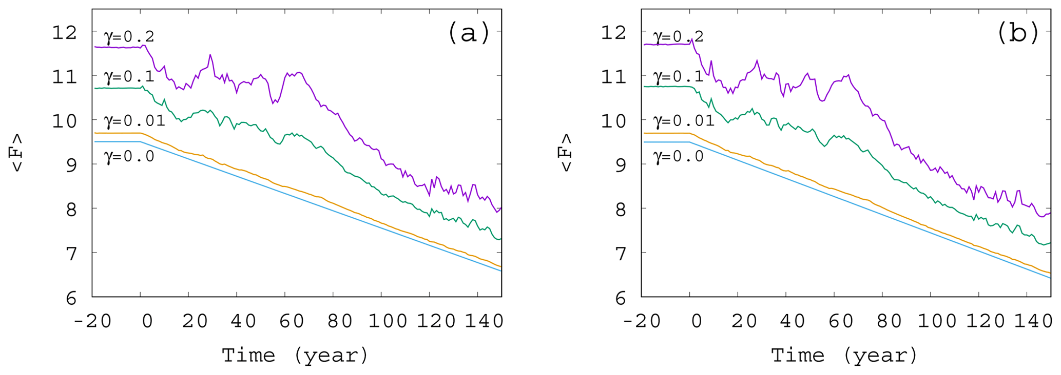
Figure 3Time dependence of the ensemble-averaged atmospheric forcing in the case of , and 0.2 for (a) α=0.05 and (b) . The slope of the blue line for γ=0 corresponds to D in Eq. (12).
It is visible in the inset to Fig. 2b that the ensemble average curve shows some change during the first 5 years (between and −15 years). This indicates (along with several other simulations; not shown) that the convergence to the snapshot attractor takes about tc=5 years. The numerical data after years thus represent parallel atmosphere–phytoplankton realizations on the snapshot attractor of the system.
The considerable deviation of the individual time series from the ensemble average indicates that the formers are not representing properly the mean climate state, as also pointed out by Drótos et al. (2015). Therefore, from here on, we shall concentrate on ensemble averages and consider the variance in these as a measure of the internal variability (the size of the snapshot attractor in the chosen variable).
We carried out similar simulations with other extraction parameter values from the range and found that β does not have much effect on the average phytoplankton concentration, and the curves for various values of β are close to each other (see Fig. S1 in the Supplement Sect. S2). In what follows, therefore, we stick to a single value, β=0.1.
The time dependence of the typical (ensemble-averaged) temperature contrast forcing the atmospheric variables in Eq. (1) is shown in Fig. 3. The value of at each time instant is computed from Eqs. (4) and (8), with the average values (ensemble average over 50 000 trajectories at that time instant) in place of c. The fluctuations in the curve of Fig. 3 follow the fluctuations in the average phytoplankton concentration, but, for small values of γ, the linear decrease in F(t) is recovered. In other words, for weak mixing (small values of γ) the trend in the forcing F(t) follows quite closely the direct anthropogenic trends. For strong mixing (γ≥0.1), however, the fluctuations have longer timescale; hence the trends imposed by anthropogenic effects are less obvious, in particular, on shorter timescales. A comparison of Fig. 3a and b belonging to α=0.05 and , respectively, indicates that a change in the sign of the enrichment parameter leads to only minor differences in the general trends.
Next, we study the dependence of the ensemble average of the phytoplankton concentration on the strength of mixing. We have seen in Fig. 2 that for γ=0.1 strong deviations appear from the trend, αD0, occurring without mixing. The time dependence of for mixing parameters on this order of magnitude, shown in Fig. S2, confirms the existence of large fluctuations. The time dependence of for much smaller values of γ are shown in Fig. 4. The linearly increasing trend in harmony with Eqs. (10) and (11) gradually disappears, and large-scale fluctuations are visible even for γ=0.005.

Figure 4Ensemble-averaged phytoplankton concentration as a function of time for α=0.05 for various values of γ (γ=0, 0.001, 0.002, 0.003, 0.004, and 0.005). The thick red line shows the expected phytoplankton concentration in lack of mixing (γ=0) as predicted by Eq. (11).
It seems that even a small coupling of the atmospheric variables x, y, and z to the phytoplankton dynamics will result in large variations in and in the suppression of the anthropogenic trends on short terms. One can also conclude from these figures that a coupling with γ≥0.002 should already be considered strong in the atmosphere–ocean interaction, at least from the point of view of the phytoplankton dynamics.
Now we investigate the effect of the enrichment parameter α on the phytoplankton concentration. We have seen in Fig. 4 that for small α=0.05, the short-term trends are destroyed for γ>0.002. We see in Fig. 5 that with an increase in , a trend might reappear at even higher values of the mixing parameter γ=0.01. Indeed, for α between roughly −0.05 and 0.05, no trend is visible, and large scale fluctuations stemming from the internal variability in the dynamics rule the behavior of the average phytoplankton population. For , however, we see that trends emerge. There is an increasing trend for positive and a decreasing trend for negative α with a slope similar to the one given by the analytic calculation valid for γ=0.
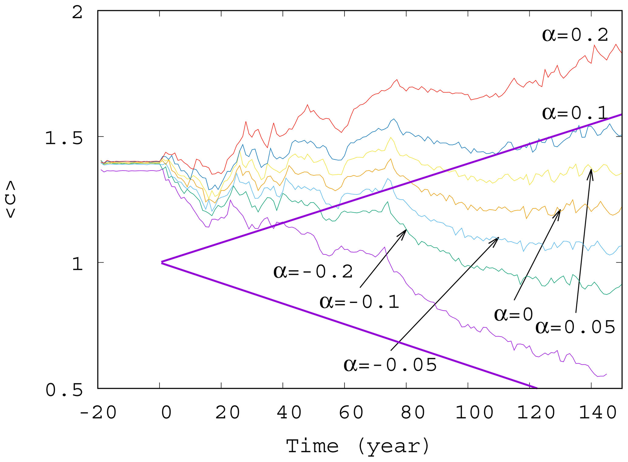
Figure 5Average phytoplankton concentration as a function of time for γ=0.01 for various values of α (−0.2, −0.1, −0.05, 0.0, 0.05, 0.1, and 0.2). The thick purple lines show the expected phytoplankton concentration without mixing (γ=0) as predicted by Eq. (11) for (lower line) and α=0.2 (upper line).
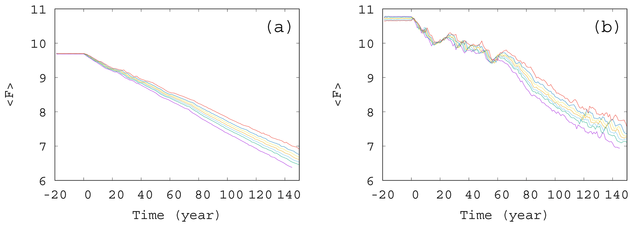
Figure 6Time dependence of the average forcing in the case of (a) γ=0.01 and (b) γ=0.1. The values of the enrichment parameter from top to bottom are α=0.2, 0.1, 0.05, 0, −0.05, −0.1, and −0.2.
From the same set of α values used to construct Fig. 5, we show the time dependence of the average forcing for an intermediate (γ=0.01) and a large (γ=0.1) mixing parameter in Fig. 6a and b, respectively. Interestingly, for each value of α and γ, the graphs show a nearly linear decay, the slope depending somewhat on α. It seems that the direct anthropogenic component is dominant in the average forcing term, in particular for γ=0.01, but this also holds qualitatively for γ=0.1 (see Fig. 6b). We thus conclude that a mixing parameter on the order of 0.1 is not yet strong from the point of view of the forcing. This is in harmony with the observation that the atmospheric kinetic energy hardly depends on the mixing strength (see Fig. S3): the atmosphere is rather resistant to the feedback from the biomass.However, an increased (decreased) amount of phytoplankton present in the system results in an increased (decreased) temperature contrast, and hence, in a decreased (enhanced) climate change, this effect is quite small. The order of magnitude of the effect of the phytoplankton concentration on can be assessed by observing in Fig. 5 that () falls between −0.5 and 1 at t=150 years. Multiplied by our fixed β=0.1, as Eq. (4) requires, one finds a range of 0.15, which is much smaller than the final value of F, about 7, at 150 years. This is comparable with the spread of the temperature contrast at the end of year 150 in Fig. 6a and b. Note that these conclusions are drawn from the average temperature contrast. No trend can be extracted if instantaneous values of a single simulation are used instead of the ensemble average, in the same spirit as in Fig. 2a.
Next, we study quantitatively how the trend observed in the ensemble average of the phytoplankton concentration changes with the parameters. To this end, we fit a straight line to the time dependence of the ensemble average of the phytoplankton concentration for t>0 for various values of parameters α and γ. The slope S(α,γ) of the best-fit line in the presence of mixing gives information on the trend of the phytoplankton concentration, that is, on how quickly the concentration changes with time on (ensemble) average. We have also computed the standard deviations of this fit from the measured values to gain information on the fluctuations appearing in individual members of the ensemble. We found (not shown) that in case of a strong trend (slope of time dependence far from zero) we find small fluctuations and vice versa.
In Fig. 7 we show the approximate slope S(α,γ) of the curves as a function of the mixing parameter γ. We see that the measured slopes, that is, the trends in the time dependence, decrease with increasing values of γ. We also found that the fluctuations (not shown) are enhanced when γ increases. This implies that when mixing becomes stronger, the phytoplankton concentration is not only decreasing for any α (the slope is negative) but also drops even faster (the slope is decreasing). Note that the initial concentration from which the decrease starts at t=0 is higher for larger γ (stronger mixing); see Figs. 4 and S2. Concerning the fluctuations, we call the attention to the fact that in nearly all figures exhibiting time dependence one can observe a decrease in the amplitude of variations for longer times, for t>100 years approximately. This appears to be a consequence of the decrease in the total atmospheric kinetic energy with time, due to the overall decrease in the temperature contrast in time, as Fig. S3 also illustrates. At a fixed mixing parameter γ, the strength of mixing is proportional to the kinetic energy, which is thus decreasing in time. Since the carrying capacity is assumed to linearly depend on the kinetic energy (see Eq. 9), K also decreases in time. Thus, the phytoplankton concentration and its fluctuations are also decreasing with time.
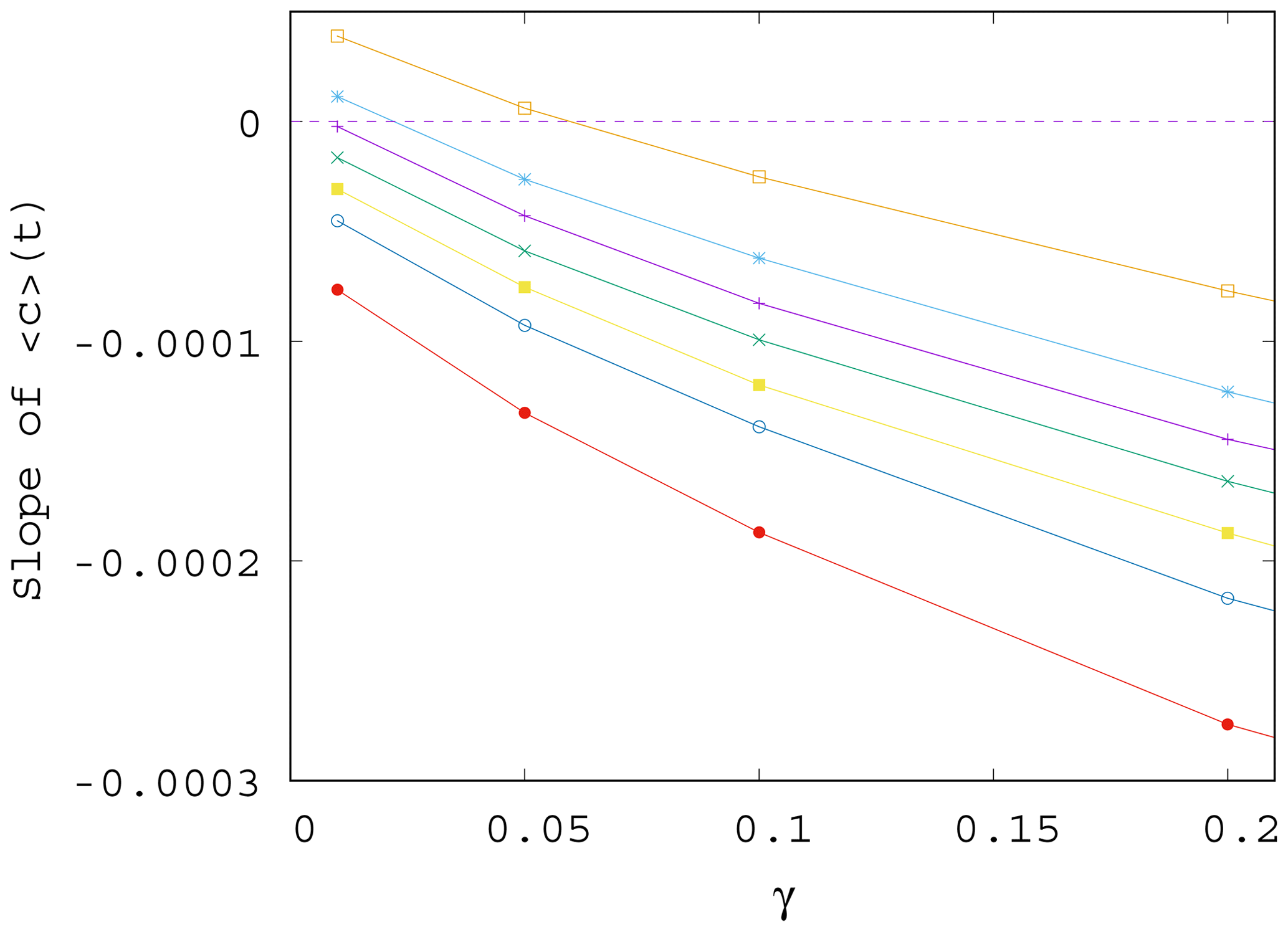
Figure 7Slope S of the ensemble average of the phytoplankton concentration, , for t>0 as γ is varied; data shown for various values of α, from top to bottom, α=0.2, 0.1, 0.05, 0, −0.05, −0.1, and −0.2.
It is worth also noting that even if for γ=0 the trend in would be increasing for positive enrichment parameters – see Eq. (11) – it is the increase in γ that converts all trends to be negative. It remains true, however, that the trend for a positive α is less negative than for a negative α. In other words, for sufficiently strong mixing, the phytoplankton concentration always decreases with time due to climate change, and the sign of the enrichment parameter only influences the strength of decrease.
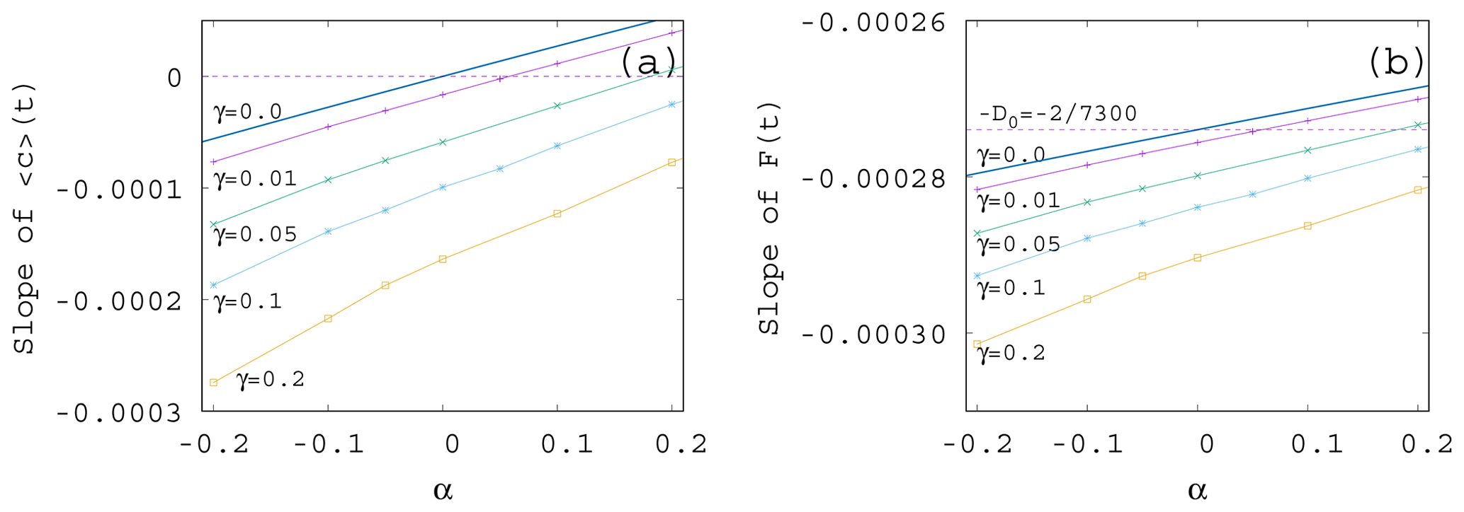
If we plot the same data shown in Fig. 7 as a function of α instead of γ – see Fig. 8a – we see that the increase in the enrichment parameter increases the trend in the phytoplankton concentration. It is a surprising observation that even if the change in the mixing parameter changes the slopes essentially, their α dependence remains similarly linear as for γ=0 given in Eq. (11). Plotting the slope of the time-dependent, ensemble-averaged forcing as a function of α – see Fig. 8b – a very weak dependence is found (note the vertical scale). On a closer look, the α dependence is linear and increasing. This is in harmony with the expectation that the CO2 extraction is weaker when the phytoplankton concentration is lower. With the exception of small γ values, the slopes are more negative than the direct anthropogenic one, −D0. It is a remarkable finding supported by our results that a large mixing parameter enhances the speed of the climate change, irrespective of the sign of the enrichment parameter.
We see that the trends predicted by Eqs. (11) and (12) are approached when γ is decreased. What is even more interesting, the dependence of the trends on α remains the same for any γ. In particular, we find a numerical fit of the slope S of for β=0.1 as
A similar expression is obtained from the slopes of the averaged forcing that replaces D0 found in Eq. (12) for γ=0 by
It is surprising that the leading-order linear behavior in the enrichment parameter α found for S and D without any mixing remains valid for practically the entire γ range investigated; just the coefficients become γ dependent.
The mathematical concepts underlying the ensemble view are snapshot (Romeiras et al., 1990) or pullback (Ghil et al., 2008) attractors. One might consider the ensemble of all permitted climate realizations over all times as the pullback attractor of the problem and the set of the permitted states of the climate at a given time instant as the snapshot attractor belonging to that time instant (their union over all time instants is the pullback attractor). Both views express that the climate system possesses a plethora of possibilities. In the terminology of climate science, climate has a strong internal variability (e.g., Stocker et al., 2013). The concept of snapshot or pullback attractors is nothing but a reformulation of this fact in dynamical terms.
In numerical simulations, we consider the members of an ensemble simulation to describe parallel climate realizations only after the initial conditions are “forgotten”, and transient dynamics disappears. Due to dissipation, this time is typically short compared to the time span of interest. Such an ensemble approach was shown to be the only method providing reliable statistical predictions in systems with underlying nonpredictable dynamics (since in this class the traditional approach based on a single time series is known to provide seriously biased results). A number of papers illustrate these statements within the physics literature (see, e.g., Romeiras et al., 1990; Lai, 1999; Serquina et al., 2008), as well as in low-order climate models (Chekroun et al., 2011; Bódai et al., 2011; Bódai and Tél, 2012; Bódai et al., 2013; Drótos et al., 2015), in general circulation models (Haszpra and Herein, 2019; Kaszás et al., 2019; Pierini et al., 2018, 2016; Drótos et al., 2017; Herein et al., 2017; Bódai et al., 2020; Haszpra et al., 2020b, a), and also in experimental situations (Vincze, 2016; Vincze et al., 2017).
For several parameter values, we also determined the snapshot attractors of the coupled model. An example is given in Fig. 9 where we see the attractor on the z=0 slice of the atmospheric dynamics with the corresponding c values not shown directly. Different colors indicate different time instances separated by 10 years, clearly indicating that the attractor is changing in time. As the colors indicate, the projection to the x–y plane of the z=0 cross section of the snapshot attractor has a minimum size in years 60–80, after which it increases again, and the maximum extension is reached by about year 150. Note that one cannot decide how much of the time dependence is a consequence of F0(t) or the phytoplankton concentration. Due to the couplings between the biomass and the atmosphere, the direct anthropogenic effect cannot be separated from the effect of the biomass.
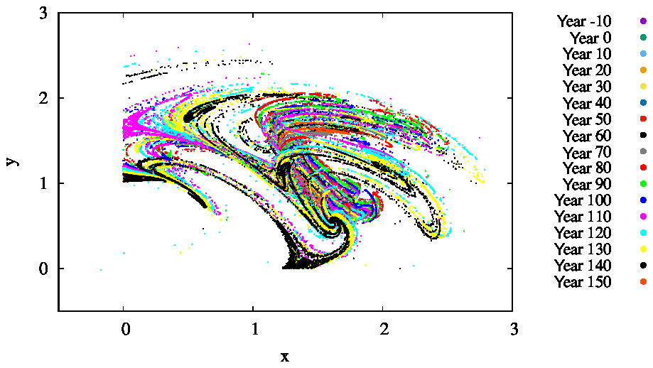
Figure 9The projection of the z=0 and section of the snapshot attractors on the x–y plane for β=0.1, α=0.05, and γ=0.1. The snapshot attractors at intervals of 10 years are shown with purple ( years), green (t=0 years), cyan (t=10 years), light orange (t=20 years), yellow (t=30 years), dark cyan (t=40 years), dark red (t=50 years), dark grey (t=60 years), grey (t=70 years), red (t=80 years), light green (t=90 years), blue (t=100 years), pink (t=110 years), light blue (t=120 years), bright yellow (t=130 years), black (t=140 years), and dark orange (t=150 years). They are generated by initiating 7×10⁷ random initial conditions at year −20.
By investigating a projection of the snapshot attractor on a plane containing concentration c as one of the axes, the influence of mixing on the internal variability within c can be visualized. In Fig. 10, the z=0 slice of the snapshot attractor of a given time instant is shown for three values of γ, projected to the x–c plane; that is, the y values are not shown. We see that the extension of the snapshot attractor in the c direction is greatly affected by the strength of mixing: the c extension is zero for γ=0 but increases rapidly for increasing γ. Parallel to this, the pattern becomes interwoven in the space of variables, suggesting that the c dynamics becomes more and more complex in time, too. It is the increasing size and complexity of the snapshot attractor in the c direction which is reflected in the increase in the strength of fluctuations in Figs. 4 and S2.
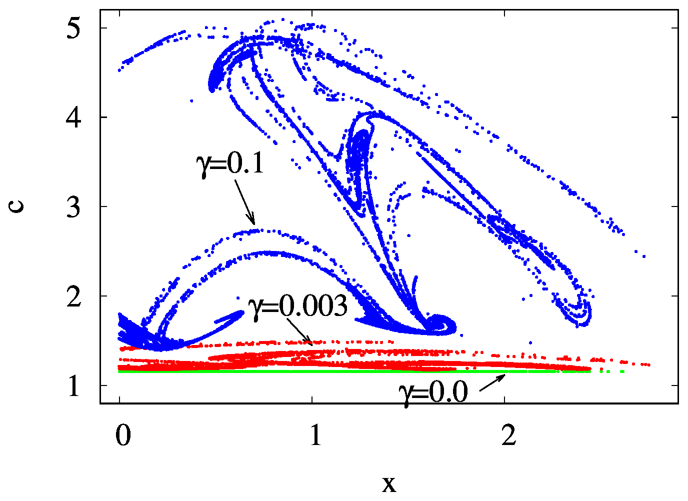
Figure 10The projection of the z=0 and section of the snapshot attractors at year 150 on the x–c plane for β=0.1 and α=0.05 and for γ=0.0 (green), 0.003 (red), and 0.1 (blue).
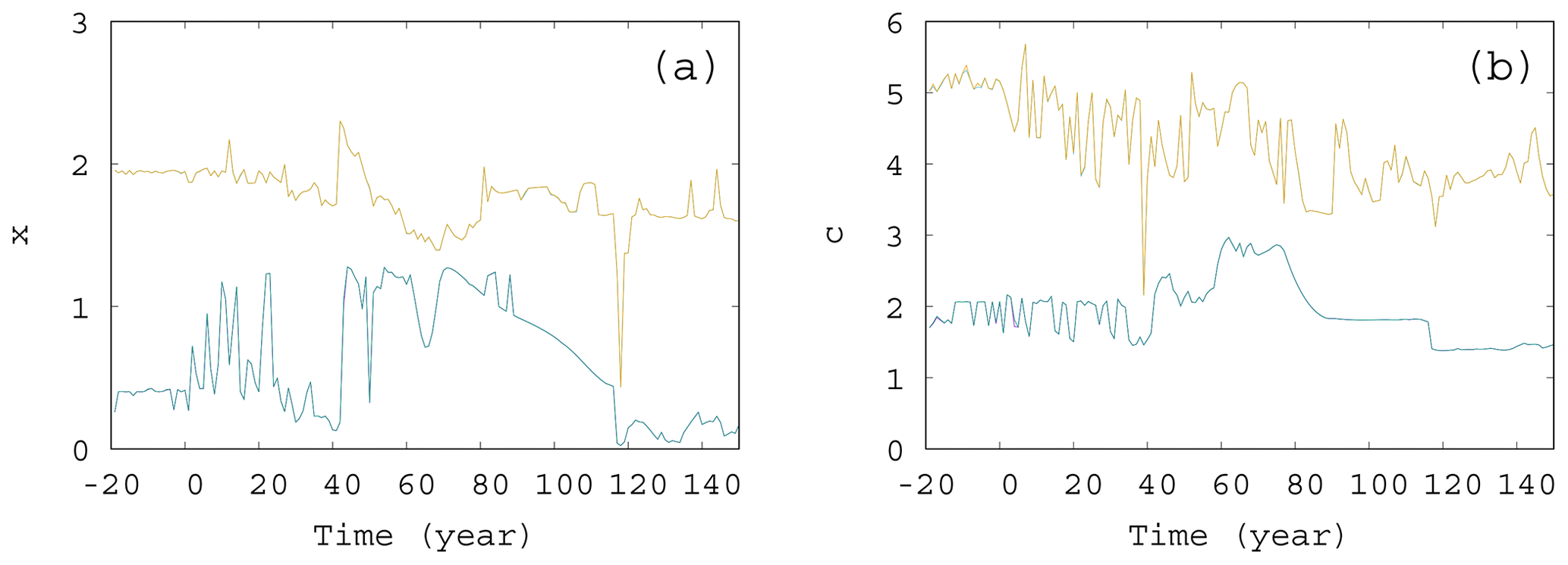
Figure 11The extremes of the snapshot attractor for α=0.05, β=0.1, and γ=0.1. Only 10 % of the points are found above (below) the higher (lower) values for each time instant for (a) x and (b) c.
We also investigated the extremes of the snapshot attractors. That is, at a fixed time instant, we looked for those values of, e.g., x, for which only 10 % of values can be found on the snapshot attractor below (lower extreme) or above (higher extreme) x. These values of x are shown in Fig. 11a as a function of time. The interval between these thresholds is a measure of the size of the extension of the snapshot attractor at a given time instant. Clearly, this size undergoes strong variations as a function of time. The same is shown in Fig. 11b for the time dependence of the c extension of the snapshot attractor: the upper (lower) curve shows the value of c, above (below) which only 10 % of the values appear on the snapshot attractor. Again, we see considerable variations in time. It is interesting to note that, as these figures indicate, there is no unique trend in the size of the snapshot attractors, although trends can be seen in averages taken with respect to the ensemble designating the attractor itself, like, e.g., in or .
We have set up a conceptual coupled atmosphere–phytoplankton model by combining the Lorenz'84 general circulation model and the logistic equation under the condition of a climate change due to a linear decrease in the strength of direct anthropogenic forcing. The novel features of the model are in the choice of the possible forms of couplings. We allow for an influence of the biomass on the atmospheric forcing, modeling this way the extractions of CO2 by phytoplankton, but the same forcing is able to modify the carrying capacity via its coupling to the temperature contrast characterized by the enrichment parameter. An additional atmosphere–ocean coupling is also taken into account mimicking the enhancement of phytoplankton primary production via increased atmospheric activity, i.e., via turbulent mixing. Our intention has been to include leading-order effects, and hence the coupling constants are chosen intentionally to be small. Nevertheless, interesting consequences are found.
By investigating the parameter dependence of the ensemble average of the atmospheric forcing and the phytoplankton content, we have shown that
-
even without mixing, the phytoplankton biomass interacts with the atmospheric forcing, and the coupling between the phytoplankton concentration and the temperature might weaken or strengthen the anthropogenic warming trend; the increase or decrease in the phytoplankton biomass depends on the sign of the enrichment parameter. In this regime, analytic results are available; see Eqs. (10), (11) and (12).
-
increased mixing parameter enhances the total phytoplankton population biomass. Stronger coupling may enhance fluctuation to a degree that the anthropogenic component practically disappears (Figs. 4 and S2).
-
in contrast, mixing appears to depress the trend of the extraction of CO2 by phytoplankton and may force the phytoplankton population to globally decrease in time (see Fig. 7), although starting from a higher initial level.
-
the coupling of mixing with phytoplankton biomass has a much weaker effect on the atmospheric forcing (see Fig. 6), as it is minimally expected from a coupled atmosphere–phytoplankton model.
-
despite the strong modifications due to mixing, the dependence of trends on the strength of the coupling between the phytoplankton concentration and the temperature (the enrichment parameter) remains practically the same as without mixing (see Fig. 8).
We have obtained these results in a conceptual coupled atmosphere–phytoplankton model which contains a tractable number of variables and parameters. To our knowledge, this is the first attempt to understand the general and robust features of the interplay between the atmosphere and the biosphere in a climate change framework. One of our main results is that an increase in the global temperature reduces mixing intensity, which is the leading factor in decreasing the total biomass of phytoplankton. Interestingly, this result is in concordance with numerous studies applying Earth system models with vastly more detailed plankton models (Bopp et al., 2013; Fu et al., 2016; Kwiatkowski et al., 2019), although other works report different observations (Laufkötter et al., 2015; Flombaum et al., 2020).
As far as we know, our work is the first step in the direction of studying the feedbacks between the atmosphere and the biosphere by a simple conceptual model. Our conclusions are robust in a mathematical sense, meaning that small changes in our model (inclusion of noise, for example) will not alter our main findings, since snapshot attractors are robust. As long as the addition of other interactions only provide a small perturbation, our conclusions remain valid. In general, it is an open question in complex nonlinear systems whether neglected couplings to other subsystems and other simplifications could cause qualitative change in the dynamical behavior of a model. However, we see two important reasons why we believe our model goes in the right direction. First, the trends we find in our model are in accordance with the trends observed in the majority of complex models as mentioned above. Second, we believe that in our model the origin of trends is more transparent than in more complex models where this origin can be hidden among the multitude of variables, feedbacks, and interactions. Our model is a conceptual model, and as such, both the biological and climate models are highly simplified. However, one can consider it as a starting module of an extendable model system. On the one hand, more trophical levels and inorganic resources can be easily added to the biological side of our model; on the other hand, simple ocean circulation models can extend the climate side of our model in order to make a first step to build more complex coupled models (Daron and Stainforth, 2013). We think that mutual interactions and iterations between conceptual models and detailed Earth system models (ESM) help to reveal the distinction between relevant and less relevant mechanisms and feedbacks behind climate change. We expect deeper insight into these feedbacks by studying conceptual models and ESMs parallelly in the future.
The C language code applied during the simulations is included in the Supplement.
The supplement related to this article is available online at: https://doi.org/10.5194/esd-11-603-2020-supplement.
GK, IS, and TT worked out the outline of the applied model, with a special contribution of IS to the biological background; GK and TT carried out the analytical calculations; GK developed the simulation code; GK and RDP carried out the simulations; all authors contributed to the preparation of the paper.
The authors declare that they have no conflict of interest.
We are thankful for the useful comments from Tamás Bódai, Gábor Drótos, and Tímea Haszpra. This work was supported by the National Research, Development and Innovation Office of Hungary under grant K-125171. István Scheuring is supported by Hungary's Economic Development and Innovation Operative Program (GINOP 2.3.2-15-2016-00057). György Károlyi is supported by grant BME FIKP-VÍZ of EMMI.
This research has been supported by the NKFIH (grant no. K-125171), the GINOP (grant no. 2.3.2-15-2016-00057), and the EMMI (grant no. BME FIKP-VÍZ).
This paper was edited by Ben Kravitz and reviewed by two anonymous referees.
Basu, S. and Mackey, K. R. M.: Phytoplankton as Key Mediators of the iological Carbon Pump: Their Responses to a Changing Climate, Sustainability, 10, 869, https://doi.org/10.3390/su10030869, 2018. a, b
Blunden, J. and Arndt, D. S.: State of the climate in 2012, B. Am. Meteorol. Soc., 94, S1–S258, 2013. a
Bódai, T. and Tél, T.: Annual variability in a conceptual climate model: Snapshot attractors, hysteresis in extreme events, and climate sensitivity, Chaos, 22, 023110, https://doi.org/10.1063/1.3697984, 2012. a
Bódai, T., Károlyi, Gy., and Tél, T.: A chaotically driven model climate: extreme events and snapshot attractors, Nonlin. Processes Geophys., 18, 573–580, https://doi.org/10.5194/npg-18-573-2011, 2011. a
Bódai, T., Károlyi, Gy., and Tél, T.: Driving a conceptual model climate by different processes: Snapshot attractors and extreme events, Phys. Rev. E, 87, 022822, https://doi.org/10.1103/PhysRevE.87.022822, 2013. a
Bódai, T., Drótos, G., Herein, M., Lunkeit, F., and Lucarini, V.: The Forced Response of the El Niño–Southern Oscillation–Indian Monsoon Teleconnection in Ensembles of Earth System Models, J. Climate, 33, 2163–2182, 2020. a
Bopp, L., Resplandy, L., Orr, J. C., Doney, S. C., Dunne, J. P., Gehlen, M., Halloran, P., Heinze, C., Ilyina, T., Séférian, R., Tjiputra, J., and Vichi, M.: Multiple stressors of ocean ecosystems in the 21st century: projections with CMIP5 models, Biogeosciences, 10, 6225–6245, https://doi.org/10.5194/bg-10-6225-2013, 2013. a
Chekroun, M. D., Simonnet, E., and Ghil, M.: Stochastic climate dynamics: Random attractors and time-dependent invariant measures, Phys. D, 240, 1685–1700, 2011. a
Chust, G., Allen, J. I., Bopp, L., Schrum, C., Holt, J., Tsiaras K., Zavatarelli, M., Chifflet, M., Cannaby, H., Dadou, I., Daewel, U., Wakelin, S. L., Machu, E., Pushpadas, D., Butenschon, M., Artioli, Y., Petihakis, G., Smith, C., Garçon, V., Goubanova, K., Le Vu, B., Fach, B. A., Salihoglu, B., Clementi, E., and Irigoien, X.: Biomass changes and trophic amplification of plankton in a warmer ocean, Glob. Change Biol.,20 2124–2139, https://doi.org/10.1111/gcb.12562, 2014. a
Daron, J. D. Stainforth, D. A.: On predicting climate under climate change, Environ. Res. Lett., 8, 034021, https://doi.org/10.1088/1748-9326/8/3/034021, 2013. a
De La Rocha, C. L. and Passow, U.: The Biological Pump, Treatise on Geochemistry, 8, 93–122, https://doi.org/10.1016/B978-0-08-095975-7.00604-5, 2014. a
Drótos, G., Bódai, T., and Tél, T.: Probabilistic concepts in a changing climate: A snapshot attractor picture, J. Climate, 28, 3275–3288, 2015. a, b, c, d, e, f, g
Drótos, G., Bódai, T., and Tél, T.: On the importance of the convergence to climate attractors, Eur. Phys. J.-Spec. Top., 226, 2031–2038, 2017. a
Estrada, M. and Berdalet, E.: Phytoplankton in a turbulent world, Sci. Mar., 61, 125–140, 1997. a
Falkowski, P. G.: Biogeochemistry of Primary Production in the Sea, Treatise on Geochemistry, 10, 163–187, https://doi.org/10.1016/B978-0-08-095975-7.00805-6, 2014. a
Falkowski, P. G., Barber, R. T., and Smetacek, V.: Biogeochemical controls and feedbacks on ocean primary production, Science, 281, 200–206, 1998. a
Falkowski, P., Scholes, R. J., Boyle, E., Canadell, J., Canfield, D., Elser, J., Gruber, N., Hibbard, K., Hogberg, P., Linder, S., Mackenzie, F. T., Moore III, B., Pedersen, T., Rosenthal, Y., Seitzinger, S., Smetacek, V., and Steffen, W.: The global carbon cycle: A test of our knowledge of Earth as a system, Science, 290, 291–296, 2000. a
Falkowski, P. G., Laws, E. A., Barber, R. T., and Murray, J. W.: Phytoplankton and their role in primary, new, and export production, in: Ocean Biogeochemistry. Global Change – The IGBP Series, edited by: Fasham, M. J. R., Springer, Berlin, Heidelberg, Germany, 2003. a
Flombaum, P., Wang, W.-L., Primeau , F. W., and Martiny, A. C.: Global picophytoplankton niche partitioning predicts overall positive response to ocean warming, Nat. Geosci., 13, 116–120, 2020. a
Fu, W., Randerson, J. T., and Moore, J. K.: Climate change impacts on net primary production (NPP) and export production (EP) regulated by increasing stratification and phytoplankton community structure in the CMIP5 models, Biogeosciences, 13, 5151–5170, https://doi.org/10.5194/bg-13-5151-2016, 2016. a
Ghil, M.: Climate stability for a Sellers-type model, J. Atmos. Sci., 33, 3–20, 1976. a
Ghil, M., Chekroun, M. D., and Simonnet, E.: Climate dynamics and fluid mechanics: Natural variability and related uncertainties, Phys. D, 237, 2111–2126, 2008. a
Guidi, L., Chaffron, S., Bittner, L., Eveillard, D., Larhlimi, A., Roux, S., and Gorsky, G.: Plankton networks driving carbon export in the oligotrophic ocean, Nature, 532, 465–470, https://doi.org/10.1038/nature16942, 2016. a
Hader, D. P., Villafane, V. E., and Helbling, E. W.: Productivity of aquatic +primary producers under global climate change, Photochem. Photobiol. Sci., 13, 1370–1392, 2014. a
Haszpra, T. and Herein, M.: Ensemble-based analysis of the pollutant spreading intensity induced by climate change, Sci. Rep., 9, 3896, https://doi.org/10.1038/s41598-019-40451-7, 2019. a
Haszpra, T., Herein, M., and Bódai, T.: Investigating ENSO and its teleconnections under climate change in an ensemble view – a new perspective, Earth Syst. Dynam., 11, 267–280, https://doi.org/10.5194/esd-11-267-2020, 2020a. a
Haszpra, T., Topál, D., and Herein, M.: On the Time Evolution of the Arctic Oscillation and Related Wintertime Phenomena under Different Forcing Scenarios in an Ensemble Approach, J. Climate, 33, 3107–3124, 2020b. a
Herein, M., Drótos, G., Haszpra, T., Marfy, J., and Tél, T.: The theory of parallel climate realizations as a new framework for teleconnection analysis, Sci. Rep., 7, 44529, https://doi.org/10.1038/srep44529, 2017. a
Hutchins, D. A. and Fu, F.: Microorganisms and ocean global change, Nat. Microbiol., 2, 17058, https://doi.org/10.1038/nmicrobiol.2017.58, 2017. a
Jäger, C. G., Diehl, S., and Emans, M.: Physical Determinants of Phytoplankton Production, Algal Stoichiometry, and Vertical Nutrient Fluxes, Am. Nat., 175, E91–E104, 2010. a
Kaszás, B., Haszpra, T., and Herein, M.: The snowball Earth transition in a climate model with drifting parameters: Splitting of the snapshot attractor, Chaos, 29, 113102, https://doi.org/10.1063/1.5108837, 2019. a
Kwiatkowski, L., Aumont, O., and Bopp L.: Consistent trophic amplification of marine biomass declines under climate change, Glob. Change Biol., 25, 218–229, 2019. a
Lai, Y.-C.: Transient fractal behavior in snapshot attractors of driven chaotic systems, Phys. Rev. E, 60, 1558–1562, 1999. a
Laufkötter, C., Vogt, M., Gruber, N., Aita-Noguchi, M., Aumont, O., Bopp, L., Buitenhuis, E., Doney, S. C., Dunne, J., Hashioka, T., Hauck, J., Hirata, T., John, J., Le Quéré, C., Lima, I. D., Nakano, H., Seferian, R., Totterdell, I., Vichi, M., and Völker, C.: Drivers and uncertainties of future global marine primary production in marine ecosystem models, Biogeosciences, 12, 6955–6984, https://doi.org/10.5194/bg-12-6955-2015, 2015. a, b
Li, W., Gao, K. S., and Beardall, J.: Interactive effects of ocean acidification and nitrogen-limitation on the diatom phaeodactylum tricornutum, PLoS ONE, 7, e51590, https://doi.org/10.1371/journal.pone.0051590, 2012. a
Lorenz, E. N.: Irregularity: A fundamental property of the atmosphere, Tellus, 36A, 98–110, https://doi.org/10.1111/j.1600-0870.1984.tb00230.x, 1984. a, b
Lorenz, E. N.: Can chaos and intransitivity lead to interannual variability?, Tellus, 42A, 378–389, https://doi.org/10.1034/j.1600-0870.1990.t01-2-00005.x, 1990. a, b
Mackey, K. R. M., Morris, J. J., Morel, F. M. M., and Kranz, S. A.: Response of Photosynthesis to Ocean Acidification, Oceanography, 28, 74–91, https://doi.org/10.5670/oceanog.2015.33, 2015. a
Marinov, I., Doney, S. C., and Lima, I. D.: Response of ocean phytoplankton community structure to climate change over the 21st century: partitioning the effects of nutrients, temperature and light, Biogeosciences, 7, 3941–3959, https://doi.org/10.5194/bg-7-3941-2010, 2010. a
Mongwe, N. P., Vichi, M., and Monteiro, P. M. S.: The seasonal cycle of pCO2 and CO2 fluxes in the Southern Ocean: diagnosing anomalies in CMIP5 Earth system models, Biogeosciences, 15, 2851–2872, https://doi.org/10.5194/bg-15-2851-2018, 2018. a
Peters, F. and Marrasé, C.: Effects of turbulence on plankton: an overview of experimental evidence and some theoretical considerations, Mar. Ecol. Prog. Ser., 205, 291–306, 2000. a
Pierini, S., Ghil, M., and Chekroun, M.D.: Exploring the pullback attractors of a low-order quasigeostrophic ocean model: The deterministic case, J. Climate, 29, 4185–4202, 2016. a
Pierini, S., Chekroun, M. D., and Ghil, M.: The onset of chaos in nonautonomous dissipative dynamical systems: a low-order ocean-model case study, Nonlin. Processes Geophys., 25, 671–692, https://doi.org/10.5194/npg-25-671-2018, 2018. a
Reid, P. C., Fischer, A. C., Lewis-Brown, E., Meredith, M. P., Sparrow, M., Andersson, A. J., Antia, A., Bates, N. R., Bathmann, U., Beaugrand, G., Brix, H., Dye, S., Edwards, M., Furevik, T., Gangstø, R., Hátún, H., Hopcroft, R. R., Kendall, M., Kasten, S., Keeling, R., Le Quéré, C., Mackenzie, F. T., Malin, G., Mauritzen, C., Olafsson, J., Paull, C., Rignot, E., Shimada, K., Vogt, M., Wallace, C., Wang, Z., and Washington, R.: Chapter 1. Impacts of the oceans on climate change, Adv. Mar. Biol., 56, 1–150, https://doi.org/10.1016/S0065-2881(09)56001-4, 2009. a
Roberts, C. M., O'Leary, B. C., McCauley, D. J., Cury, P. M., Duarte, C. M., Lubchenco, J., Pauly, D., Sáenz-Arroyo, A., Rashid Sumaila, U., Wilson, R. W., Worm, B., and Castilla, J. C.: Marine reserves can mitigate and promote adaptation to climate change, P. Natl. Acad. Sci. USA, 114, 6167–6175, https://doi.org/10.1073/pnas.1701262114, 2017. a
Romeiras, F. J., Grebogi, C., and Ott, E.: Multifractal properties of snapshot attractors of random maps, Phys. Rev. A, 41, 784–799, 1990. a, b
Sanders, R., Henson, S. A., Koski, M., De la Rocha, C. L., Painter, S. C., Poulton, A. J., Riley, J., Salihoglu, B,. Visser, A., Yool, A., Bellerby, R., and Martin, A. P.: The biological carbon pump in the north Atlantic, Prog. Oceanogr., 129, 200–218, 2014. a
Schlunegger, S., Rodgers, K. B., Sarmiento, J. L., Frölicher, T. L., Dunne, J. P., Ishii, M., and Slater, R.: Emergence of anthropogenic signals in the ocean carbon cycle, Nat. Clim. Chang., 9, 719–725, 2019. a
Serezze, M. C. and Francis, J. A.: The Arctic amplification debate, Climate Change, 76, 241–264, https://doi.org/10.1007/s10584-005-9017-y, 2006. a
Serquina, R., Lai, Y.-C., and Chen, Q.: Characterization of nonstationary chaotic systems, Phys. Rev. E, 77, 026208, https://doi.org/10.1103/PhysRevE.77.026208, 2008. a
Stocker, T. F., Qin, D., Plattner, G.-K., Tignor, M. M. B, Allen, S. K., Boschung, J., Nauels, A., Xia, Y., Bex, V., and Midgley, P. M.: The Physical Science Basis. Contribution of Working Group I to the Fifth Assessment Report of the Intergovernmental Panel on Climate Change, Cambridge University Press, Cambridge, UK, New York, USA, 2013. a
Stommel, H.: Thermohaline convection with two stable regimes of flow, Tellus, 13, 224–230, 1961. a
Sverdrup, H. U.: On conditions for the vernal blooming of phytoplankton, Journal du Conseil International pour l'Exploraton de la Mer, 18, 287–295, 1953. a
Tél, T., Bódai, T., Drótos, G., Haszpra, T., Herein, M., Kaszás, B., and Vincze, M.: The theory of parallel climate realizations: A new framework of ensemble methods in a changing climate – an overview, J. Stat. Phys., https://doi.org/10.1007/s10955-019-02445-7, 2019. a
Turner, J. T.: Zooplankton fecal pellets, marine snow, phytodetritus and the ocean’s biological pump, Prog. Oceanogr., 130, 205–248, 2005. a
Vincze, M.: Modeling climate change in the laboratory, in: Teaching Physics Innovatively, edited by: Király, A. and Tél, T., 107–118, 2016. a
Vincze, M., Borcia, I. D., and Harlander, U.: Temperature fluctuations in a changing climate: an ensemble-based experimental approach, Sci. Rep., 7, 254, https://doi.org/10.1038/s41598-017-00319-0, 2017. a
Whitt, D. B., Taylor, J. R., and Levy, M.: Synoptic-to-planetary scale wind variability enhances phytoplankton biomass at ocean fronts, J. Geophys. Res.-Oceans, 122, 4602–4633, https://doi.org/10.1002/2016JC011899, 2017. a
Wilson, J. D., Monteiro, F. M., Schmidt, D. N., Ward, B. A., and Ridgwell, A.: Linking Marine Plankton Ecosystems and Climate: A New Modeling Approach to theWarm Early Eocene Climate, Paleoceanography and Paleoclimatology, 33, 1439–1452, https://doi.org/10.1029/2018PA003374, 2018. a
Zhong, Y., Liu, Z., and Notaro, M: A GEFA Assessment of Observed Global Ocean Influence on U.S. Precipitation Variability: Attribution to Regional SST Variability Modes, J. Climate, 24, 693–707, https://doi.org/10.1175/2010JCLI3663.1, 2011. a