the Creative Commons Attribution 4.0 License.
the Creative Commons Attribution 4.0 License.
 | 12 May 2020
Differing precipitation response between solar radiation management and carbon dioxide removal due to fast and slow components
Peter K. Snyder
Stefan Liess
Antti-Ilari Partanen
Dylan B. Millet
Solar radiation management (SRM) and carbon dioxide removal (CDR) are geoengineering methods that have been proposed to mitigate global warming in the event of insufficient greenhouse gas emission reductions. Here, we have studied temperature and precipitation responses to CDR and SRM with the Representative Concentration Pathway 4.5 (RCP4.5) scenario using the MPI-ESM and CESM Earth system models (ESMs). The SRM scenarios were designed to meet one of the two different long-term climate targets: to keep either global mean (1) surface temperature or (2) precipitation at the 2010–2020 level via stratospheric sulfur injections. Stratospheric sulfur fields were simulated beforehand with an aerosol–climate model, with the same aerosol radiative properties used in both ESMs. In the CDR scenario, atmospheric CO2 concentrations were reduced to keep the global mean temperature at approximately the 2010–2020 level. Results show that applying SRM to offset 21st century climate warming in the RCP4.5 scenario leads to a 1.42 % (MPI-ESM) or 0.73 % (CESM) reduction in global mean precipitation, whereas CDR increases global precipitation by 0.5 % in both ESMs for 2080–2100 relative to 2010–2020. In all cases, the simulated global mean precipitation change can be represented as the sum of a slow temperature-dependent component and a fast temperature-independent component, which are quantified by a regression method. Based on this component analysis, the fast temperature-independent component of the changed atmospheric CO2 concentration explains the global mean precipitation change in both SRM and CDR scenarios. Based on the SRM simulations, a total of 163–199 Tg S (CESM) or 292–318 Tg S (MPI-ESM) of injected sulfur from 2020 to 2100 was required to offset global mean warming based on the RCP4.5 scenario. To prevent a global mean precipitation increase, only 95–114 Tg S was needed, and this was also enough to prevent global mean climate warming from exceeding 2∘ above preindustrial temperatures. The distinct effects of SRM in the two ESM simulations mainly reflected differing shortwave absorption responses to water vapour. Results also showed relatively large differences in the individual (fast versus slow) precipitation components between ESMs.
- Article
(9358 KB) - Full-text XML
-
Supplement
(4451 KB) - BibTeX
- EndNote


It is now widely recognized that fast greenhouse gas (GHG) emission reductions, especially for carbon dioxide (CO2), are needed if ongoing global warming is to be slowed down. The Intergovernmental Panel on Climate Change (IPCC) Special Report on Global Warming of 1.5 ∘C (henceforth SR15; IPCC, 2018) brought to wider attention the many risks and partly irreversible negative impacts associated with global mean warming of 1.5 ∘C above the preindustrial level (Liu et al., 2018; Schleussner et al., 2016; Seneviratne et al., 2018). The aim of the 2015 Paris Agreement was to maintain the global mean temperature increase within 2 ∘C of the preindustrial level and to pursue efforts to limit the mean increase to 1.5 ∘C (UNFCCC, 2015). Based on average results of climate models, only one of the Representative Concentration Pathway (RCP) scenarios used in the IPCC Fifth Assessment report (IPCC, 2014) is associated with global mean warming of less than 2 ∘C; this pathway includes presumptive mitigation after the year 2010, which has not taken place (van Vuuren et al., 2007). Millar et al. (2017) and Rogelj et al. (2018) have shown that limiting warming to 1.5 ∘C is still possible, but it would require a fast and significant reduction in the use of fossil fuels complemented with carbon dioxide removal. In addition, air quality legislation will likely lead to decreased cooling from anthropogenic aerosols, which might by itself be enough to increase global mean temperatures over the 1.5 ∘C target (Hienola et al., 2018).
Geoengineering methods have been proposed to prevent dangerous climate warming if CO2 emissions are not reduced quickly enough (e.g. Caldeira et al., 2013). Such techniques are usually divided into two categories. One is carbon dioxide removal (CDR), whereby CO2 is removed from the atmosphere, thus addressing the root cause of climate warming (Royal Society, 2009). While these actions will face many political, economic, and technical challenges, they are most likely needed in some form to avoid 1.5 ∘C warming (Luderer et al., 2018; IPCC, 2018). The second is solar radiation management (SRM), which aims to increase the shortwave (solar) reflectivity of the atmosphere or Earth's surface. The Paris agreement states that the 2 ∘C target should be achieved by reaching a balance between anthropogenic GHG emissions and anthropogenic GHG sinks (i.e. CDR) (UNFCCC, 2015). However, challenges related to mitigation and CDR, the possible underestimation of future carbon budgets, or new findings in the scientific understanding of tipping points could lead to increased interest in using SRM to avoid crossing the Paris Agreement temperature thresholds.
Discussions related to SR15 and the Paris Agreement have concentrated mainly on global mean temperature change rather than on regional variations in temperature changes (Collins et al., 2018; Seneviratne et al., 2018) or on other climate impacts, such as changes in precipitation, that are driven by temperature changes or caused directly by GHG or other forcing agents. On the global scale, precipitation changes can be separated into a surface-temperature-dependent slow component, which does not depend on the forcing agent causing the underlying temperature change, and a temperature-independent fast component, which is caused directly by the altered atmospheric radiation absorption (Bala et al., 2009; Myhre et al., 2017; Samset et al., 2016). Changes to the hydrological cycle thus depend not only on the degree of warming but also on the forcing agents and emission changes that are causing the warming. As a result, different emission pathways can lead to different precipitation changes even if they result in similar global mean temperatures. Such hydrologic changes may have a larger impact on human well-being than changes in temperature due to impacts on floods, droughts, water resources, and ecosystems (Lausier and Jain, 2018).
Problems and side effects associated with SRM have been discussed extensively (Robock et al., 2009; Royal Society, 2009). One fundamental problem is that compensating for GHG-induced warming with SRM would decrease global mean precipitation through the direct radiative effect described above. This can be understood as follows. Given a GHG concentration increase, less outgoing longwave (LW) radiation escapes to space, causing surface temperatures to increase until a new equilibrium is achieved. SRM methods aim to offset this temperature increase by reducing incoming shortwave (SW) solar radiation. Thus, even though the total radiative flux may be the same between an increased GHG + SRM scenario and the unperturbed climate, the atmospheric SW and LW radiative fluxes differ. This has been shown in general to lead to a decrease in global mean precipitation (Bala et al., 2008). In general, the suite of climate responses arising from a LW radiation change cannot be fully compensated for by modifying SW radiation. The use of SRM thus involves a trade-off between temperature and precipitation on the global scale.
CDR methods are considered less risky than SRM as these methods remove CO2 from the atmosphere and thus reduce the atmospheric GHG concentration (Royal Society, 2009). However, climate change is not necessarily a reversible process due to factors such as sea and glacier ice melt, sea level rise, and carbon cycle changes (Frölicher and Joos, 2010; Wu et al., 2015). In addition, climate does not adapt immediately to a change in radiative forcing. For example, due to ocean thermal inertia global temperatures will continue to change for decades or even centuries after a given radiative forcing perturbation. It is therefore important that CDR scenarios be studied to assess climate responses beyond changes to global mean temperature.
In Sect. 3 of this study the temperature and precipitation responses to CDR and SRM are simulated with two Earth system models (ESMs). The mechanisms driving global mean precipitation changes are assessed by separately examining the temperature-dependent slow response and radiatively induced fast response for differing magnitudes of SRM and CDR. This methodology can be used to better understand the impacts of CDR and SRM. Unlike in several previous studies, here the fast and slow responses are quantified by a regression method instead of a fixed sea surface temperature (SST) method (Duan et al., 2018; Myhre et al., 2017; Samset et al., 2016). An advantage of the regression method is that it separates total temperature-dependent and temperature-independent responses, while in the fixed SST method land temperature adjustments are included in the temperature-independent fast response. We also study regional disparities in temperature and precipitation responses for both geoengineering techniques and estimate the SO2 emission amounts required to keep either temperature or precipitation at present-day levels.
In Sect. 4 we simulate three geoengineering scenarios against the Representative Concentration Pathway 4.5 (RCP4.5) scenario (Thomson et al., 2011). We examine two SRM scenarios designed to address two different climate targets: keeping either global mean (1) surface temperature or (2) precipitation at the 2010–2020 level via stratospheric sulfur injections. A CDR scenario is designed to keep the global mean temperature at approximately the 2010 level. We used an aerosol–climate model to simulate stratospheric aerosol fields and two separate ESMs (MPI-ESM and CESM) to simulate the climate response to SRM and CDR.
2.1 Models
This study was conducted using three climate models: one aerosol–climate model with fixed sea surface temperature and two ESMs. We first simulated stratospheric aerosol fields with the aerosol climate model ECHAM-HAMMOZ. We then implemented the radiative properties of these fields in two ESMs – the Max Planck Institute Earth System Model (MPI-ESM) and the National Center for Atmospheric Research's Community Earth System Model (CESM) – for simulation of the various scenarios. For each scenario, we run a three-member ensemble with both ESMs.
2.1.1 ECHAM-HAMMOZ
We defined the radiative properties of the aerosol fields resulting from stratospheric injections of sulfur dioxide (SO2) with the MAECHAM6.1-HAM2.2-SALSA global aerosol–climate model (Bergman et al., 2012; Kokkola et al., 2008; Laakso et al., 2016; Stevens et al., 2013; Zhang et al., 2012). In this model, the ECHAM atmospheric module (Stevens et al., 2013) is coupled interactively with the HAM aerosol module (Zhang et al., 2012). The HAM module calculates the emissions, removal, and radiative properties of aerosols along with the associated gas- and liquid-phase chemistry. The model includes the SALSA explicit sectional aerosol scheme (Kokkola et al., 2018), which describes aerosols based on number and volume size distributions with 10 and 7 size sections for soluble and insoluble particles, respectively. The model simulates the microphysical processes of nucleation, condensation, coagulation, and hydration. The model was configured as described by Laakso et al. (2017). Simulations were performed at T63L47 resolution, which approximately corresponds to a 1.9∘ × 1.9∘ horizontal grid with 47 vertical levels reaching up to ∼80 km. The model accurately simulates stratospheric aerosol loads and radiative properties based on observations of the 1991 Mt. Pinatubo eruption (Laakso et al., 2016; Kokkola et al., 2018). It should be noted that this model configuration does not simulate the quasi-biennial oscillation at L47 resolution. The hydroxyl radical (OH), which impacts the oxidation of SO2 to sulfate and the ozone concentration, is accounted for through prescribed monthly mean fields.
2.1.2 MPI-ESM and CESM
MPI-ESM (Giorgetta et al., 2013) consists of the same atmospheric model (ECHAM6.1) as ECHAM-HAMMOZ, and the MPI-ESM simulations here also employed the same T63L47 resolution as the ECHAM-HAMMOZ simulations described above. MPI-ESM includes the JSBACH active land model (Reick et al., 2013) and the Max Planck Institute Ocean Model (MPIOM) (Jungclaus et al., 2013), both fully coupled to the atmospheric module. MPIOM includes the HAMOCC ocean biogeochemistry model (Ilyina et al., 2013). The tropospheric aerosol climatology of Kinne et al. (2013) is used in all scenarios.
CESM version 1.2.2 (Hurrell et al., 2013) consists of the Community Atmospheric Model (CAM4), which is used with a horizontal resolution of 0.9∘ × 1.25∘ and 26 vertical levels up to 40 km (finite-volume grid). It is coupled to the Parallel Ocean Program (POP2) ocean model, the Community Land Model (CLM4), and Community Ice CodE (CICE4) sea ice model.
2.1.3 Implementing prescribed aerosol fields in ESMs
To examine the effects of solar radiation management by stratospheric sulfur injections, we implemented prescribed sulfate fields in ESMs as described by Laakso et al. (2017). First, we used ECHAM-HAMMOZ to simulate aerosol fields resulting from gaseous SO2 injections. These simulations include a 2-year spin-up period followed by a 5-year steady-state period. From this 5-year period, aerosol optical depth (AOD), single-scattering albedo (SSA), and the asymmetry factor (ASYM) were archived as monthly output in 14 SW bands plus absorption AOD in 16 LW bands. We then implemented these fields in the two ESMs as prescribed zonal and monthly mean fields. ECHAM-HAMMOZ and MPI-ESM share the ECHAM atmosphere model, which itself uses the Rapid Radiative Transfer Model. Because the same resolution (T63L47) was employed for both ECHAM-HAMMOZ and MPI-ESM, the only differences in aerosol radiative properties between the models were caused by zonal and monthly averaging of the radiative properties (however, the total AOD did not vary between the two). In the case of CESM, aerosol fields from the ECHAM-HAMMOZ simulations had to be interpolated horizontally to 0.9∘ × 1.25∘ and to 26 vertical levels. Because CAM4 uses different wavelength bands than ECHAM (7 LW bands and 19 SW bands), we interpolated the aerosol optical properties accordingly.
The above implementation ensures that SRM radiative effects are consistent in both ESMs, while also enabling longer-term analyses since computationally expensive aerosol microphysics are prescribed rather than simulated online. The aerosol radiative effects are nevertheless based on explicit simulations of aerosol microphysics and of the resulting aerosol size distribution and spatial–temporal variability. Our methodology is therefore more physically realistic compared to approaches that simply reduce the solar constant or apply idealized zonally homogenous aerosol fields. Realistic simulation of aerosol microphysics is necessary for robust prediction of the associated radiative effects, which depend on the size, properties, and location of the particle. In the stratosphere, particle lifetimes are roughly 1 year so that microphysical processes such as coagulation and condensation play a greater role than in the troposphere. As a result of these microphysical processes, radiative forcing from stratospheric sulfur injections does not increase linearly with the amount of injected sulfur, and thus radiative impacts cannot be scaled linearly based on the injection level (Niemeier and Timmreck, 2015).
2.2 Simulations
To simulate SRM stratospheric aerosol fields, we performed six SRM and one control simulation with ECHAM-HAMMOZ. Here, SO2 was injected continuously throughout the simulation at 20 km of altitude between 10∘ N and 10∘ S latitude. Each of the ECHAM-HAMMOZ simulations included the injection of 1, 2, 3, 4, 5, or 6 Tg S yr−1.
We divide the ESM simulations into two groups: (1) component analysis simulations and (2) scenarios. Component analysis simulations are performed to enable subsequent separation of the slow (temperature-dependent) and fast (temperature-independent) responses to the specific forcing agent based on a regression method (Gregory et al., 2004). In this method, an individual forcing agent (CO2 or SRM) is added to the steady-state climate conditions, and different climate variables are regressed against the global mean surface temperature change. The fast and slow responses for a specific forcing agent are then obtained from the fitted regression line. Specifically, the fast temperature-independent response is derived as the intercept (zero temperature change), while the slow temperature-dependent response is derived as the slope. This analysis is done for three purposes: (1) to evaluate the implementation of the stratospheric aerosol fields across the two ESMs, (2) to quantify differences in radiative forcing and climate sensitivity between models under a specific forcing agent, and (3) to separate the fast and slow precipitation responses of the forcing agents. A total of nine scenarios are simulated with both ESMs: preindustrial, six SRM scenarios with 1, 2, 3, 4, 5, and 6 Tg S injections, and 2×CO2 and 4×CO2 conditions.
All component analysis simulations start from a radiatively balanced climate for preindustrial conditions. A forcing agent (CO2 or SRM) is introduced at the outset of the simulation, while other conditions are kept at preindustrial levels. We simulated three 20-year ensemble members for each component analysis scenario in Table 1.
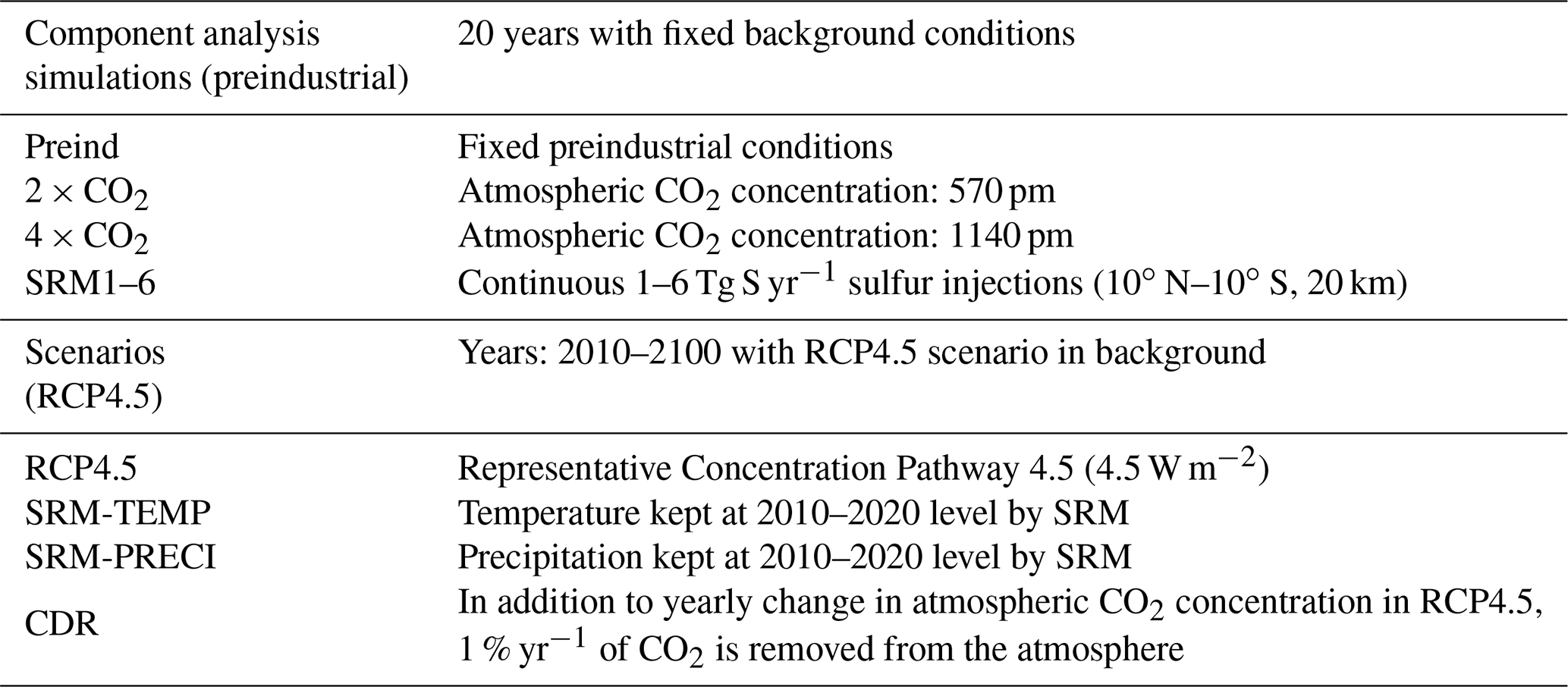
Scenario simulations were based on RCP4.5 (Moss et al., 2010; van Vuuren et al., 2011) and included the following: (i) one baseline scenario with no geoengineering (RCP4.5), (ii) two SRM scenarios designed to keep global mean surface temperature (SRM-TEMP) or precipitation (SRM-PRECI) at 2010–2020 mean values, and (iii) one CDR scenario designed to keep global mean surface temperature at the 2010–2020 mean value (CDR). In each case, three ensemble members were simulated for the years 2010–2100.
In the RCP4.5 scenario, radiative forcing stabilizes several decades before the end of the simulations (year 2100), leading to warming clearly below that seen in the high emission scenario (RCP8.5) but above the targets defined in the Paris Agreement. For the SRM-TEMP and SRM-PRECI scenarios, the global mean temperature or precipitation was kept close to the 2010–2020 mean by changing the level of stratospheric sulfur injections.
In practice, the SRM-TEMP and SRM-PRECI objectives were achieved by adjusting the aerosol loading as needed based on the continuous SO2 injection simulations from ECHAM-HAMMOZ (Sect. 2.1.3). Specifically, the SRM was controlled annually based on mean temperature or precipitation values from the two preceding years, as follows:
where X2010−2020 is the global mean temperature (SRM-TEMP) or precipitation (SRM-PRECI) for 2010–2020 based on RCP4.5. represents the corresponding global mean value in the two preceding years. A running window of two preceding years is used to avoid undue influence from natural variability in global mean temperature or precipitation. Use of a longer window is suboptimal because the temperature or precipitation change the year following an SRM adjustment then does not carry sufficient weight for the subsequent evaluation. This can lead to overly large temperature or precipitation changes before the need to act is recognized.
The A parameter is a threshold value set to 0.2 K in SRM-TEMP, which based on our test simulations is generally larger than natural variability. For SRM-PRECI, A is defined to correspond to a 0.5 % change in the global mean precipitation in the model. If both of the above conditions are false, the stratospheric sulfur injections are maintained at the previous year's level. SRM simulations are initialized with 1 Tg S yr−1 injections at year 2020.
An approximation inherent in this approach is that transitory ramp-up and ramp-down periods in the stratospheric aerosol burden with 1 Tg S yr−1 changes in SRM are not taken into account. Thus, the simulated SRM changes take place faster than would occur in the real world. For example, the ECHAM-HAMMOZ simulation with 5 Tg S yr−1 injections requires 6 months to achieve 70 % of the ultimate steady-state AOD (533 nm) after starting from background conditions. When sulfur injections are suspended in the ECHAM-HAMMOZ simulation, the AOD decreases by roughly by 40 % over the course of the first year. However, since the sulfur changes in our ESM simulations are only ±1 Tg S yr−1 and do not usually occur in consecutive years, we can assume that neglecting this time lag does not significantly alter our overall results.
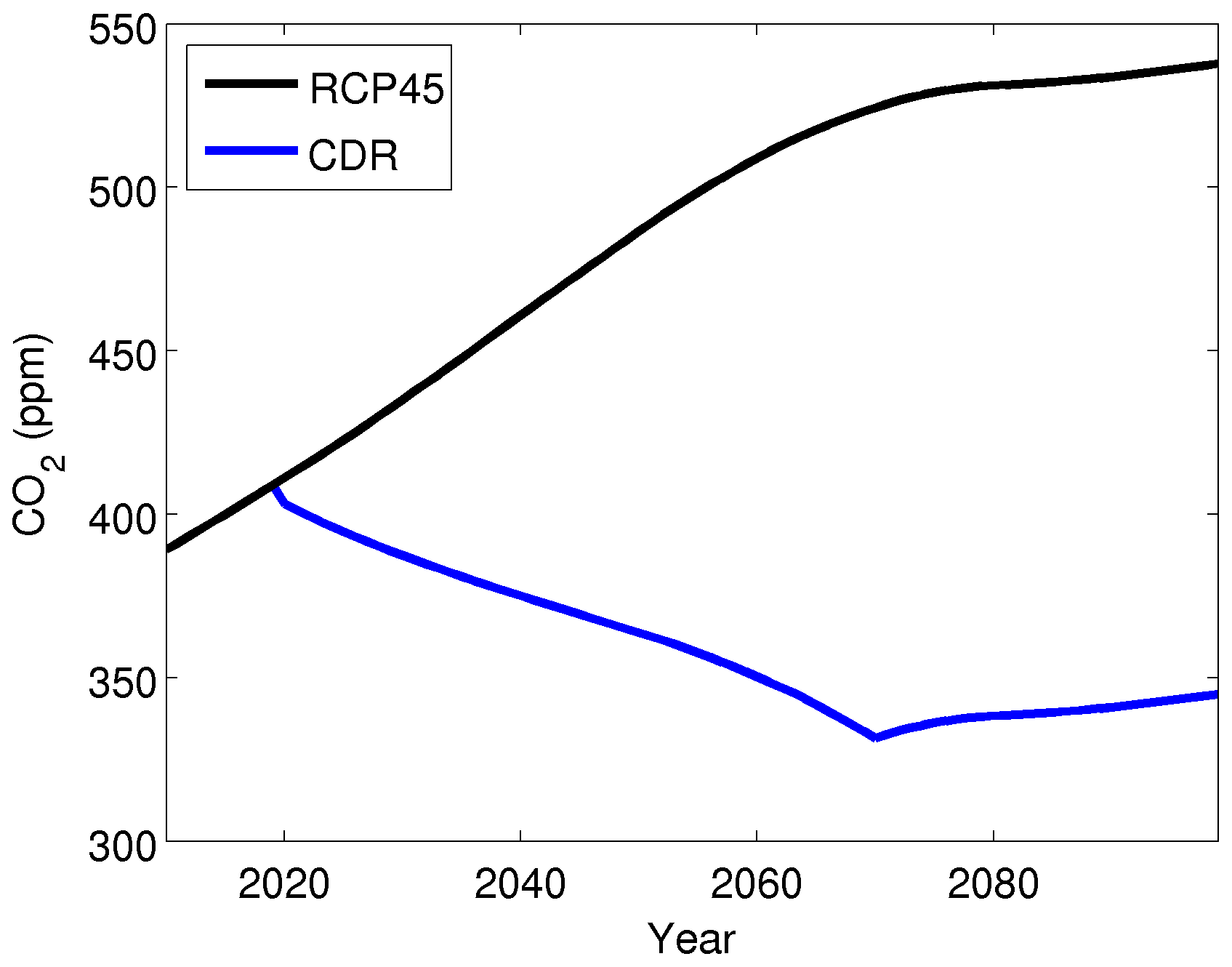
In the CDR scenarios, CO2 removal was likewise initialized at the year 2020. Here, the annual CO2 increase based on RCP4.5 was counteracted by a 1 % annual removal of the atmospheric CO2 concentration. This process was continued until the year 2070, when radiative forcing is stabilized in the RCP4.5 scenario. Accounting for both RCP4.5 emissions and CDR, the total atmospheric CO2 concentration is then reduced yearly by 0.3 %–0.6 % between 2020 and 2070 (Fig. 1). Removing 1 % of atmospheric CO2 in 2020 corresponds to negative emissions of approximately 8.7 Gt C yr−1. As carbon cycle feedbacks (i.e. outgassing from natural carbon sinks) lower the efficiency of CDR (Tokarska and Zickfeld, 2015), the actual amount of sequestered carbon would in reality need to be even higher than this. Achieving such high negative emissions in 2020 would be virtually impossible. The rate required is higher than the maximum estimated sustainable potential of the highest-potential negative emission technologies (Fuss et al., 2018), without even considering competition between the methods. Among SR15 scenarios pursuing the most aggressive CDR, the median carbon sequestration rate for the primary employed method (bioenergy with carbon capture and storage) reaches ∼4 Gt C yr−1 in 2100 (Rogelj et al., 2018). Thus, the CDR scenario employed here should be considered an idealized high-end carbon removal scenario, and we do not speculate how CDR could be achieved and do not study the impacts of any specific CDR technology. All non-CO2 GHG concentrations and other forcings in the CDR scenario are the same as in RCP4.5.
The fast and slow components of radiation and precipitation were quantified from component analysis simulations by regressing the variables of interest against temperature. These simulations were 20 years long. In each case, three ensemble members were simulated. Simulations were initiated in stable preindustrial conditions. In addition, a forcing agent (CO2 or SRM) was included, which causes radiative imbalance and results in warming or cooling. Then, annual global mean values were regressed against temperature to separate temperature-dependent and temperature-independent responses.
3.1 Evaluating the implementation of stratospheric sulfur aerosol fields in MPI-ESM and CESM
We evaluated the stratospheric aerosol implementation by comparing clear-sky aerosol radiative forcing in the two ESMs with that in ECHAM-HAMMOZ. The ECHAM-HAMMOZ simulations were performed with fixed sea surface temperatures, with aerosol radiative forcing calculated based on the change between a scenario with stratospheric sulfur injection and the control simulation. To calculate the corresponding radiative forcing in the ESMs, a regression (Gregory) method was used (Gregory et al., 2004) (Fig. 2), which also provides the climate feedback parameter which can be used to analyse different responses in the two ESMs. First, we calculated the clear-sky shortwave flux and temperature anomaly compared to the stable preindustrial conditions (Preind simulation) for each year individually and performed a linear regression between the two variables. Then, we obtained a radiative forcing as the clear-sky shortwave flux anomaly of the linear regression line at zero temperature anomaly (i.e. when the climate system has not yet adjusted to the forcing).
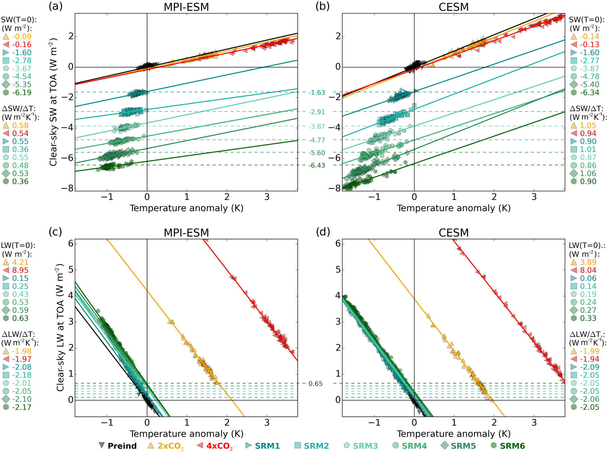
Figure 2Gregory plots of the shortwave radiative flux change (clear-sky conditions) with (a) MPI-ESM and (b) CESM, as well as of the longwave radiative flux change (clear-sky conditions) with (c) MPI-ESM and (d) CESM. Markers indicate a single-year global mean value in one ensemble member, and solid lines are linear fit lines. Dashed lines show aerosol clear-sky radiative forcing in ECHAM-HAMMOZ, with numerical values shown in the middle. Corresponding radiative forcing – the intersection of the linear fit and the y axes (T=0) – in MPI-ESM and CESM is shown at the top, and the slope of the linear fit is at the bottom of the legends next to the panels. Origin represents zero temperature and clear-sky radiative flux anomaly compared to the Preind simulation.
The SW radiative forcing in both ESMs was in good agreement with that in ECHAM-HAMMOZ (dashed lines). Radiative forcings were slightly smaller (i.e. less negative) in MPI-ESM than ECHAM-HAMMOZ, likely due to differing background conditions (preindustrial in MPI-ESM versus the year 2000 in ECHAM-HAMMOZ and thus more extensive ice cover in the MPI-ESM simulations). The zonal distribution of radiative forcing also agrees well between the models (not shown). Stratospheric aerosols absorb some LW radiation, and the LW radiative forcing in MPI-ESM agrees well with that in ECHAM-HAMMOZ. However, CESM exhibits 37 % (on average) weaker LW radiative forcing than ECHAM-HAMMOZ. This is probably due to the different radiative transfer models in CESM-CAM4 (9 LW radiation bands) and ECHAM-HAMMOZ (16 LW radiation bands). However, LW radiative forcing was small compared to the SW forcing, and this underestimation does not significantly affect the results or conclusions of this study. Since LW radiative forcing (warming effect) is weaker and SW radiative forcing (cooling) is stronger in CESM than in MPI-ESM, SRM resulted in slightly more clear-sky cooling in CESM.
We see in Fig. 2 that SW radiative forcing does not increase linearly with the amount of injected sulfur. This is because more sulfur condenses onto existing particles, and small particles coagulate more efficiently with larger particles when the sulfate burden is increased. This leads to lower particle numbers and larger particle sizes per unit of sulfur injected (Heckendorn et al., 2009; English et al., 2012; Niemeier and Timmreck, 2015). Conversely, Fig. 2 shows that the LW radiative forcing increased quite linearly with the amount of injected sulfur as shown, as also demonstrated by Niemeier and Timmreck (2015).
Earth's outgoing radiation linearly follows changes in temperature (Koll and Cronin, 2018), an effect apparent in Fig. 2c and d. However, SW radiation also changes as a function of temperature and we found that this change is fairly linear. The resulting feedback was positive, amplifying cooling in the SRM scenarios and amplifying warming in the case of a CO2 increase. The radiative fluxes in Fig. 2 are clear sky, and this SW feedback is thus caused mainly by ice cover and albedo changes along with changes in atmospheric absorption. The SW feedback was much larger in CESM (all-scenario average of 0.96 W m2 K−1) than in MPI-ESM (0.50 W m2 K−1). There was no large difference in surface albedo change between models (Fig. S1 in the Supplement). However, clear-sky SW absorption (net clear-sky SW flux at top of the atmosphere (TOA) – net clear-sky SW flux at the surface) was linearly dependent on surface temperature by 0.98 W m2 K−1 in MPI-ESM and 0.85 W m2 K−1 in CESM (Fig. S2). We attribute this to the atmospheric shortwave response of the change in atmospheric water vapour due to the temperature change. The differing model response likely originates from the distinct radiation schemes and spectral resolutions in MPI-ESM and CESM. This argument is supported by Fildier and Collins (2015), who likewise derived a larger SW absorption response to temperature in MPI-ESM compared to models that include CAM4.
Overall, we find that the clear-sky aerosol radiative forcings in the two ESMs are in good agreement with ECHAM-HAMMOZ. However, the same stratospheric sulfur fields yielded 8 % weaker (on average) total (SW + LW) clear-sky radiative forcing in MPI-ESM than in CESM.
3.2 Differences in effective radiative forcings in MPI-ESM and CESM
Figure 3 shows Gregory plots for the total TOA all-sky (clouds also taken into account) radiative forcing. In this case, the total SRM radiative forcing was 22 % weaker in MPI-ESM than in CESM. On the other hand, the radiative forcing due to increased CO2 concentrations was larger in MPI (orange and red markers in Fig. 3), but the difference was relatively small and is explained by different cloud radiative forcings between models. The impact on SW radiation was larger than it was on LW radiation. The overall result is that the same stratospheric sulfur injection led to larger and faster cooling in CESM than in MPI-ESM (Fig. 3). During the 20-year simulation period, stratospheric sulfur injections of 6 Tg S yr−1 (SRM6) led to slightly over −1 K of global mean cooling (left-most green hexagon markers in Fig. 3a) in MPI-ESM but closer to −2 K in CESM (Fig. 3b). Global mean warming after 20-year 2×CO2 and 4×CO2 simulations was consistent between the models. However, there was a nearly 2 times larger radiative imbalance in MPI-ESM compared to CESM by the end of the simulations. If these simulations reached radiative equilibrium, the climate would presumably therefore be warmer in MPI-ESM than in CESM.
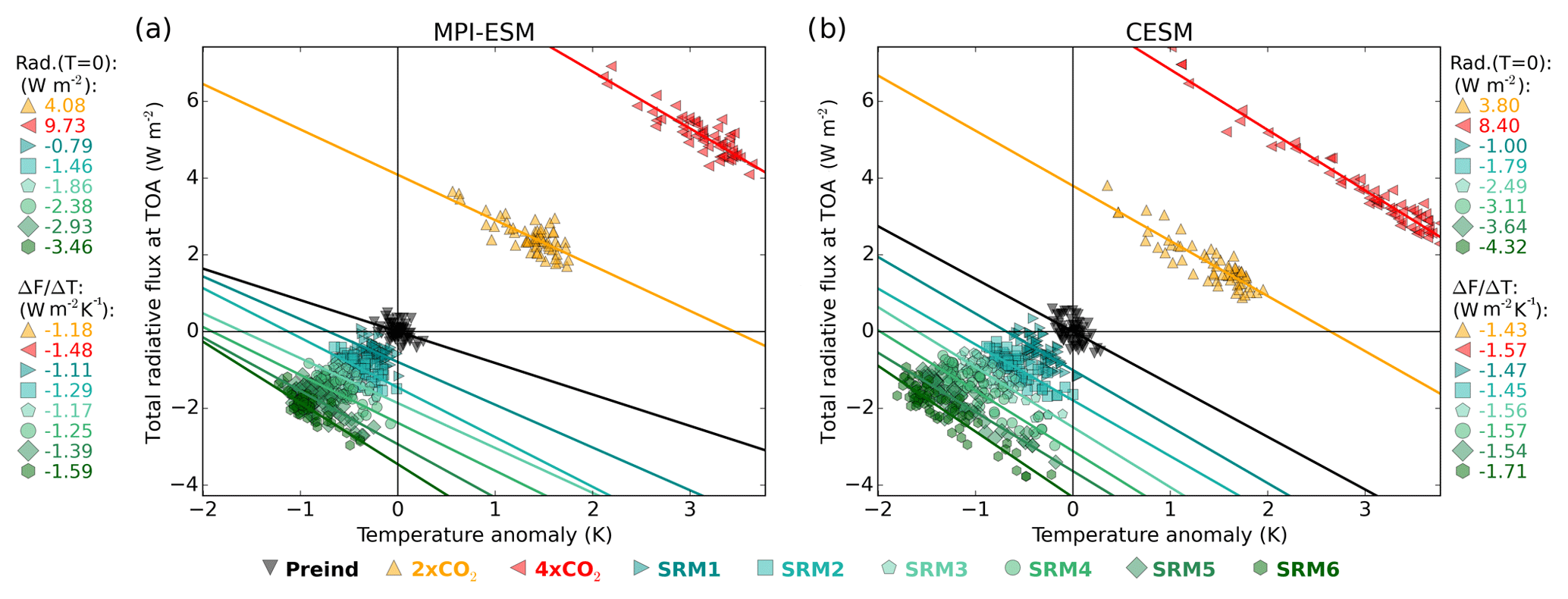
Figure 3Gregory plots of total all-sky radiative flux change at the top of the atmosphere for (a) MPI-ESM and (b) CESM. Markers indicate a single-year global mean value for one ensemble member, and solid lines are linear fits. Corresponding all-sky radiative forcing – the intersection of the linear fit and the y axes (T=0) – in MPI-ESM and CESM is shown at the top, and the slope of the linear fit is at the bottom of the legends next to the panels. Origin represents zero temperature and clear-sky radiative flux anomaly compared to the Preind simulation.
3.3 Temperature-independent fast and temperature-dependent slow precipitation responses
Precipitation responses can be divided into a temperature-independent fast response, which takes place immediately when some forcing agent is introduced, and a slow response caused by the temperature change and subsequent feedbacks (Myhre et al., 2017). Because of climate (e.g. ocean) inertia, precipitation will change slowly along with temperature even in the case of abrupt radiative forcing changes. Here, we separately quantified these fast and slow responses based on the regression method described earlier. Results are shown in Fig. 4. A fast response was obtained by the intersection of the fitted line and the y axes (T=0), and the slope of the linear fit shows the slow response due to the temperature change. Fast responses are mainly driven by changes in atmospheric absorption (Samset et al., 2016). A change in absorbed radiation modifies the amount of energy transferred between the TOA and the surface. This energy transfer is then largely compensated for by a change in latent heat flux (evaporation), in turn changing precipitation. Changes in the CO2 concentration affect LW atmospheric absorption, while SRM primarily modifies SW reflection.
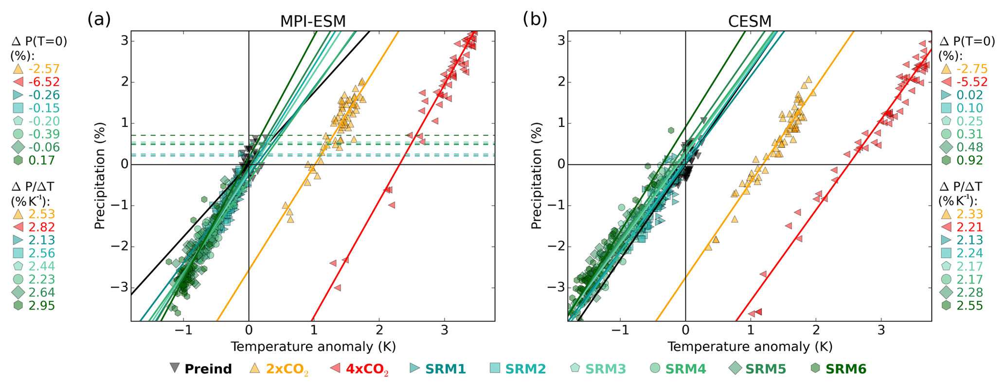
Figure 4Gregory plots of global precipitation changes under increased CO2 (orange and red) and SRM scenarios with differing sulfur injection amounts (blue to green) for (a) MPI-ESM and (b) CESM. Each marker indicates a single-year global mean value for one of three ensemble members, and solid lines are linear fits. Origin represents zero temperature and precipitation anomaly compared to the Preind simulation. A fast precipitation response is obtained from the intersection of the linear fit and the y axes (T=0) (shown at the top of the legends next to the panels), and the slope of the linear fit (shown at the bottom of the legends) corresponds to the slow response due to the temperature change. Dashed lines show (fast) precipitation responses for the corresponding scenarios in ECHAM-HAMMOZ (simulations with fixed SST).
Figure 4 shows that an atmospheric CO2 increase led immediately to a decrease in global mean precipitation. However, this CO2 increase simultaneously warms the climate, which eventually led to a precipitation increase. After 2–5 years, this temperature-dependent slow component exceeded the immediate radiative component, and global mean precipitation was then larger than in the absence of a CO2 increase. On the one hand, stratospheric sulfur aerosols (SRM1-6) also absorb some radiation (Fig. 2b) but, on the other hand, relatively more solar radiation is reflected and thus less is absorbed by the background atmosphere. We therefore saw only a small total temperature-independent increase in global mean precipitation for most SRM cases. Overall, increasing CO2 decreases precipitation via the fast component and increases precipitation via the slow temperature component (Fig. 5). Fast precipitation impacts were significantly larger for CO2 changes than for SRM (shown in the legends in Fig. 4), and therefore the fast precipitation component of SRM was omitted in Fig. 5 for clarity.
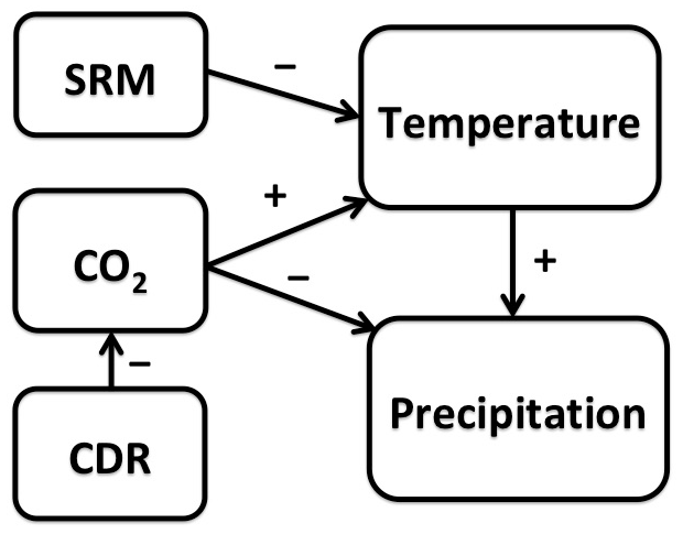
Figure 5A schematic presentation of fast radiatively induced and slow temperature-induced components of SRM and CDR. Plus and minus signs indicate the direction of change in the target variable when the driving variable is increasing. If the driving variable is decreasing (e.g. temperature decrease due to SRM), the target variable changes in the opposite direction as indicated (e.g. decrease in precipitation due to decreased temperature). The fast component of SRM is so small compared to that induced by changes in the CO2 concentration that it is omitted for clarity.
As Fig. 4a shows, the fast precipitation responses in MPI-ESM differed from those in ECHAM-HAMMOZ, despite the fact that the same atmosphere model was used in both cases. This may result from differing background conditions between the models, a land temperature change in ECHAM-HAMMOZ with fixed SST, or noise in the yearly mean values of MPI-ESM simulations.
Based on the scenarios examined here, the average global precipitation change scales with global mean temperature, with a proportionality coefficient of 2.54 % K−1 (SD 0.27 % K−1) in MPI-ESM and 2.26 % K−1 (SD 0.13 % K−1) in CESM. These values are robust for temperature changes caused by CO2 and SRM forcings. Our results thus support prior findings that the slow precipitation response is not dependent on the forcing agent (Kvalevåg et al., 2013).
In the scenario runs (Table 1), the years 2010–2100 were simulated for RCP4.5 and for geoengineering the RCP4.5 climate via SRM or CDR. Results are discussed below.
4.1 Change in global mean temperature
Global mean temperature and precipitation anomalies relative to 2010–2020 are shown in Fig. 6. Under RCP4.5, the global mean temperature increased by 1.30 and 1.20 K over the 2010–2020 average in MPI-ESM and CESM, respectively. These changes were slightly below the CMIP5 multi-model mean of 1.35 K (Knutti and Sedláček, 2012). During the same period, global mean precipitation increased by 1.76 %–1.78 % under RCP4.5, also below the CMIP5 multi-model mean (2.66 %).
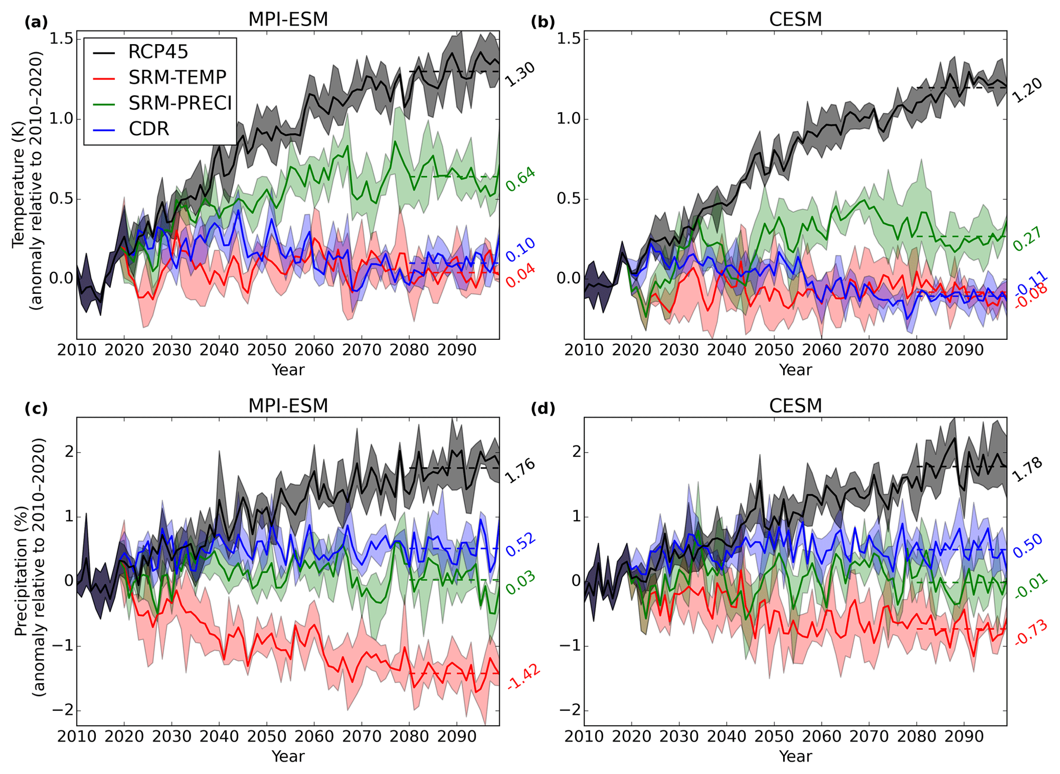
Figure 6Global mean temperature anomalies in (a) MPI-ESM and (b) CESM, as well as global mean precipitation anomalies in (c) MPI-ESM and (d) CESM. Numbers to the right of each panel indicate the global mean difference between 2080–2100 and 2010–2020. Shaded areas show the maximum and minimum across three ensemble members.
In the SRM-TEMP scenario, the global mean surface temperature was kept close to the present-day value via stratospheric sulfur injections. This reduced global mean precipitation in both ESM simulations (Fig. 6). The reduction was significantly larger in MPI-ESM (−1.42 %) than in CESM (−0.73 %). These differences are explored in Sect. 5. Given the SRM-TEMP results, it is not surprising that when global mean precipitation is maintained at the 2010 level in the SRM-PRECI scenario, the climate warms. SRM-PRECI warming in MPI-ESM is 0.64 K over the 2010–2020 level, substantially larger than was seen in CESM (0.27 K). This is consistent with the disparate model results for SRM-TEMP.
Overall, in both models, the majority of the global mean climate warming seen in RCP4.5 was compensated for in SRM-PRECI. Based on GISTEMP data, the global average temperature in 2010–2018 was approximately 1 K warmer than in the preindustrial era (defined as 1880–1900) (GISTEMP Team, 2019; Lennsen et al., 2019). Thus, in both ESMs the SRM-PRECI global temperature increase (∼1.64 K in MPI-ESM and ∼1.27 K in CESM compared to the preindustrial average) stayed within the 2 ∘C target of the Paris Agreement. For CESM, the SRM-PRECI temperature increase also stayed within the 1.5 ∘C Paris target.
The CDR scenario led to a 0.10 K (MPI-ESM) and −0.11 K (CESM) change in global mean temperature by the end of the century (2080–2100) compared to the present day (2010–2020). There was thus no significant difference in global mean temperature between the CDR and SRM-TEMP scenarios at the end of the century. The largest difference in global mean temperature between these scenarios was seen immediately after the onset of geoengineering, when the CDR temperature was larger than in SRM-TEMP. Under CDR, the global mean temperature only starts to decrease post-2040. This is because CDR acts slowly to reduce the atmospheric CO2 concentration and global temperature, whereas similar cooling can be gained with stratospheric sulfur injection much faster (Royal Society, 2009). In the CDR scenario, CO2 removal was suspended in the year 2070, when atmospheric CO2 concentrations returned to their 1976 levels. The global mean temperature at that time was close to the present-day value and did not change significantly through the end of the century (when the rate of change in atmospheric CO2 matches that seen in RCP4.5). Thus, even this very optimistic CDR scenario is insufficient for cooling the climate to pre-21st century levels. However, our CDR scenario only reduced CO2 concentrations, with other GHGs and aerosol concentrations following RCP4.5.
4.2 Change in global mean precipitation
Although the global mean surface temperature in the CDR scenario was the same at the end of the century (2080–2100) as at the beginning of the century (2010–2020), the global mean precipitation was over 0.5 % larger in both ESMs. In Sect. 3.3, we showed that the precipitation impacts of SRM and CO2 can be separated into a temperature-independent fast component and a temperature-dependent slow component. Here we use that framework to examine precipitation responses across the different geoengineering scenarios. Precipitation is also affected by non-CO2 GHGs, tropospheric aerosols, and land use changes, all of which can induce their own temperature-independent fast components. For our purposes this can be assumed to be the same across all scenarios.
Based on our component analysis simulations we see that the fast precipitation response varies fairly linearly with absorbed radiation (see Fig. S3), but some deviation occurs due to changes to sensible heat flux and physiological responses of vegetation (DeAngelis et al., 2016). This result is consistent with that of Samset et al. (2016) and Myhre et al. (2017). The higher correlations in our simulations compared to Samset et al. (2016) may be due to the use of the fixed sea surface temperature (SST) method to define the fast response in Samset et al. (2016): fast responses quantified with fixed SST methods include land temperature adjustments.
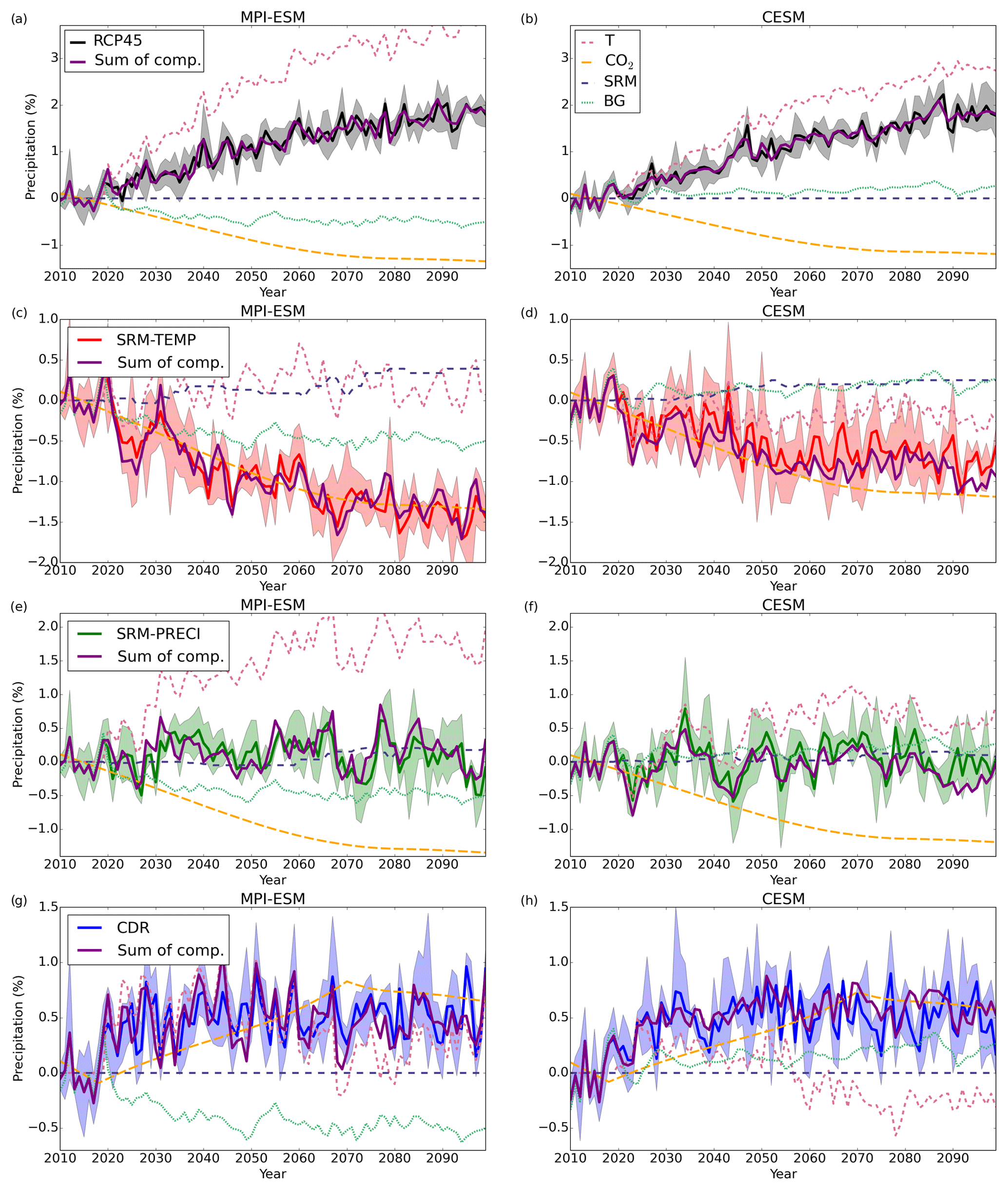
Figure 7Precipitation components for each of the simulated scenarios. Solid coloured lines with shaded areas have the same meaning as in Fig. 5c and d. Dashed coloured lines indicate the precipitation change caused by individual components (see legend in b) for each scenario and model. The purple solid line shows the sum of all precipitation components (T, SRM, CO2, and BG).
Radiative forcings are generally assumed to be additive (Marvel et al., 2015). If we assume based on Fig. S3 that the overall fast response depends only on absorbed radiation, it follows that the fast responses of individual forcing agents are also additive. In Sect. 3.3 we also showed that the slow temperature-dependent component does not depend on the applied forcing. We can thus describe the global mean precipitation change as the sum of the temperature-dependent slow component (a×ΔT) and all fast components (Fläschner et al., 2016):
where a and c are model-specific coefficients, b is a function of the SRM level, T is the simulated global mean surface temperature, CO2 preind is the preindustrial CO2 concentration, ΔCO2 is the atmospheric CO2 change relative to the preindustrial value, and BG is the background fast component, assumed to be the same for all scenarios. Coefficient a is obtained from the scenario ensemble mean slope in Fig. 4 (2.53 % K−1 for MPI-ESM and 2.27 % for CESM), while b is the fast component (intercept) from simulations of the corresponding SRM scenario (see ΔP(T=0) values in Fig. 4). To calculate coefficient c, we again assume that the fast precipitation response is linearly dependent on absorbed radiation. Radiative forcing due to CO2 varies logarithmically with concentration (Etminan et al., 2016), and thus the fast precipitation response for CO2 is also assumed to be logarithmically dependent on CO2 concentrations (see Fig. S4). We calculated the fast precipitation response for three different CO2 concentrations: preindustrial, 2×CO2, and 4×CO2. The coefficient c can then be calculated from a logarithmical fit of the fast response versus CO2 concentration across these three scenarios. This approach yields c values of 4.5 (%) for MPI-ESM and 4.0 (%) for CESM. Finally, we calculated the BG component as the 5-year running mean residual between the first three terms on the right-hand side of Eq. (2) and the modelled precipitation (ΔP in Eq. 2) based on the RCP4.5 scenario. Note that if Eq. (2) is used only to study the precipitation difference between modelled scenarios, the BG component is not needed (see Fig. S5). However, here we also wish to examine precipitation changes relative to 2010–2020, and the BG term is thus included here.
Figure 7 shows the precipitation component for each scenario in MPI-ESM and CESM. In general, the precipitation signal as estimated by the fast and slow components via Eq. (2) corresponds well to the actual model quantity in both ESMs for all scenarios. For RCP4.5 this is an obvious result because the BG is derived as the residual between the modelled precipitation and the sum of the individual components for this very scenario. However, the component-based and full precipitation signals also agree well for the other scenarios, even though the BG component is calculated from the RCP4.5 case. From the year 2020 to the year 2100 the mean differences between the Eq. (2) results and the actual model quantities ranged from −0.01 % to 0.04 % for MPI-ESM and from −0.16 % to 0.05 % for CESM. Figure S5 shows the precipitation responses under the geoengineering scenarios as anomalies relative to the RCP4.5 case. The plotted precipitation differences in Fig. S5 are thus independent of the BG component. We see from this figure that the individual components can be reliably used to understand the drivers of precipitation change for each scenario.
Figure 7a and b show that the precipitation increase in RCP4.5 would be roughly twice as large if only the slow component were operative. However, the fast radiative component reduced the global mean precipitation increase by over 1 % in both ESMs. This fast component related to increasing atmospheric CO2 (plus other GHG and absorbing aerosol) probably also explains why the increase in observed global mean precipitation has not increased significantly despite the fact that climate has warmed (Allan et al., 2014).
Under the SRM-TEMP scenario (Fig. 7c and d), the global temperature change (and thus the slow precipitation component) was small, as is the fast precipitation component due to sulfate aerosols. However, the fast component due to CO2 was as large as in RCP4.5. This fast (radiative) component from CO2 is the main reason that SRM generally leads to a decrease in global mean precipitation when used to fully offset GHG-induced warming. On the other hand, in the SRM-PRECI scenario (Fig. 7e and f) the climate was cooled to the point that the temperature-dependent slow component balances the fast radiative components (CO2, SRM, and background) so that the net precipitation change was close to zero.
The CDR scenario led to a slight increase in global mean precipitation despite no significant net change in global mean temperature. Figure 7g and f show that this was also explained by the fast radiative component of CO2. As in SRM-TEMP the slow temperature-dependent component was small. However, atmospheric CO2 concentrations were much lower by the end of the century, reducing atmospheric absorption and thus increasing global precipitation compared to 2010–2020.
Although the global mean precipitation response was approximately the same in both ESMs in RCP4.5 and CDR, a closer look at the underlying drivers shows that only the radiative component of CO2 was consistent across models. The temperature-dependent response differs between ESMs, driving divergent precipitation impacts. This resulted from a slightly different temperature response and hydrological sensitivity between ESMs. In RCP4.5 the temperature-dependent slow component was 32 % larger at the end of the simulation (2080–2100) with MPI-ESM than in the CESM simulation. In CDR the magnitude of the slow component was the same between models (0.28 % in MPI-ESM and −0.24 % in CESM at the end of the simulation), but the sign was different. However, this effect was compensated for by differing non-CO2 background responses, which also changed over the course of the simulated century. Figure 7 shows that this BG response is very different between the models and even has a different sign. In MPI-ESM non-CO2 fast components caused a 0.48 % decrease in precipitation at the end of the simulation (2080–2100) compared to the beginning (2010–2020), while in CESM non-CO2 forcers increased precipitation by 0.23 %. Thus, it is merely fortuitous that the net precipitation response was similar between models in the CDR and RCP4.5 scenarios.
The BG radiative components impacting precipitation include a range of factors such as non-CO2 GHG (methane, nitrous oxide, ozone, chlorofluorocarbons – CFCs, etc.), tropospheric and background stratospheric aerosols, and land use change – with differing treatments between models. Radiative transfer modelling also differs between the ESMs. As shown in Sect. 3.1.3, radiative forcing and (particularly) atmospheric absorption – and thus latent heat flux and precipitation – in the ESMs responded differently to the various forcing agents. Thus, it is not surprising that the BG precipitation component, which is affected by several different forcing agents, also differs between models.
Figure 8 shows the amount of sulfur required to keep global temperature or precipitation at current levels through the end of the 21st century. All scenarios started with injections of 1 Tg S yr−1 in the year 2020, and the amount of required sulfur then increased along with the RCP4.5-driven warming. In all cases, more sulfur was needed to compensate for RCP4.5 warming than for the associated precipitation increase (see the cumulative injection amount on the right-hand axes). As shown in Sect. 4.2, the fast, CO2-driven radiative component partly offsets the temperature-driven precipitation component caused by global warming. Thus, in the SRM-PRECI scenario, the sulfur aerosol only needs to compensate for the (already partly offset) precipitation effect of changing temperatures, rather than for the total temperature change (as is the case in SRM-TEMP).
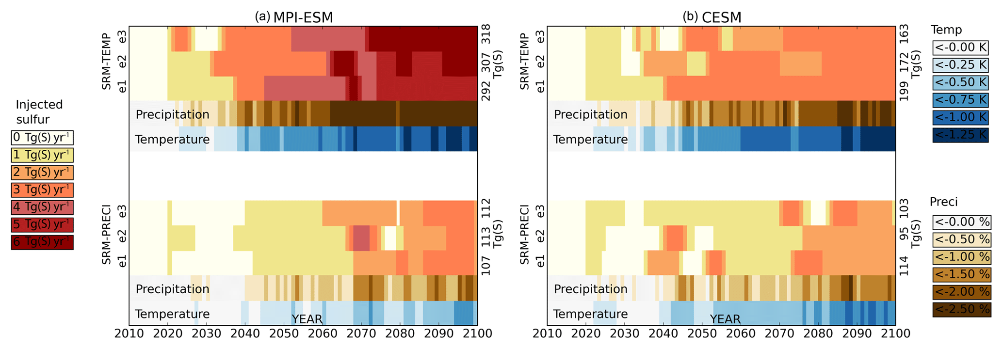
Figure 8Yearly sulfur injections in scenarios SRM-TEMP and SRM-PRECI for three ensemble members in MPI-ESM (a) and CESM (b). Also shown are the corresponding global mean precipitation and temperature differences relative to RCP4.5. The cumulative injection amount for each ensemble member is listed on the right-hand axis.
Based on these simulations, a total of 107–113 and 95–114 Tg S was required to prevent a simulated precipitation increase between the years 2020 and 2100 in MPI-ESM and CESM, respectively (scenario SRM-PRECI). These 80-year totals are slightly larger than the amount of SO2 emitted each year in the mid-1970s, when annual emissions were roughly 75 Tg S yr−1 (Smith et al., 2011). Global sulfur emissions have since decreased; however, China alone emitted over 100 Tg S SO2 between 2006 and 2008 (Li et al., 2017). However, the lifetime of aerosols derived from surface emissions is on the order of days, and the cooling impact is therefore much smaller than in the case of stratospheric injection. In the SRM-PRECI scenario, yearly injections are 3 Tg S yr−1 or less, with the exception of occasionally higher injections for one MPI-ESM ensemble member.
Figure 8 reveals significant differences in injection amounts between the two ESMs. In CESM, preventing global mean warming (under RCP4.5) through the year 2100 requires a total of 163–199 Tg S. This was less than twice the amount required to prevent an increase in global precipitation. However, simulations with MPI-ESM suggest that preventing global mean warming via SRM would require 292–318 Tg S, 50 %–100 % more than in CESM and approximately 3 times the amount required to stabilize global mean precipitation in scenario SRM-PRECI. Maximum yearly injections reached 6 Tg S yr−1 in MPI-ESM but only 3 Tg S yr−1 in CESM. These differences are mostly explained by the model responses to sulfate aerosols shown in Sect. 3: the all-sky forcing for a given amount of sulfur was significantly (22 %–33 %) larger in CESM than in MPI-ESM.
Figure 8 also shows some limitations of the climate-control algorithm used here. At times the change in the SRM injection amount was too large, leading to an overly strong climate response. In some cases the ensuing compensatory change in the injection amount then overshoots the desired climate response in the opposite direction. This led to rapid fluctuations between SRM levels, as seen, for example, between the years 2070 and 2080 in MPI-ESM ensemble member 2 for the SRM-PRECI scenario. Such effects could be avoided with smaller injection increments by using a more sophisticated algorithm that could better separate large natural variations in temperature or precipitation from long-term changes or defining the geoengineering strategy in advance by using e.g. linear response theory (Bódai et al., 2020). We also noted that the introduction of 1 Tg S yr−1 in 2020 led to an overly large precipitation response for all simulations under scenario SRM-PRECI. However, the above effects do not affect the overall results and conclusions shown here.
While the SRM-TEMP and CDR scenario simulations led to similar global mean temperatures by the end of the 21st century, the regional responses were quite different. Figure 9a and b map the temperature difference between these two scenarios in both ESMs for the last 20 years of the 21st century. We see that the SRM-TEMP scenario led to cooler tropics and warmer high latitudes than the CDR scenario in both ESMs. These regional discrepancies have been demonstrated in prior studies (Kravitz et al., 2013; Laakso et al., 2017) and point to a fundamental problem with the SRM approach. Aerosols primarily affect incoming SW radiation, while GHGs affect LW thermal radiation, and the meridional gradient is steeper for SW than for LW radiation. Consequently, compensating for a global mean LW change by modifying SW radiation leads to zonally dependent differences. This issue can be reduced by concentrating SRM injections in the middle and high latitudes or via seasonal adjustment of the sulfur injection area (Laakso et al., 2017). Overall, however, the temperature differences over land between scenarios were rarely statistically significant (indicated by hatching in Fig. 9; 10 % and 20 % of land area in MPI-ESM and CESM, respectively).
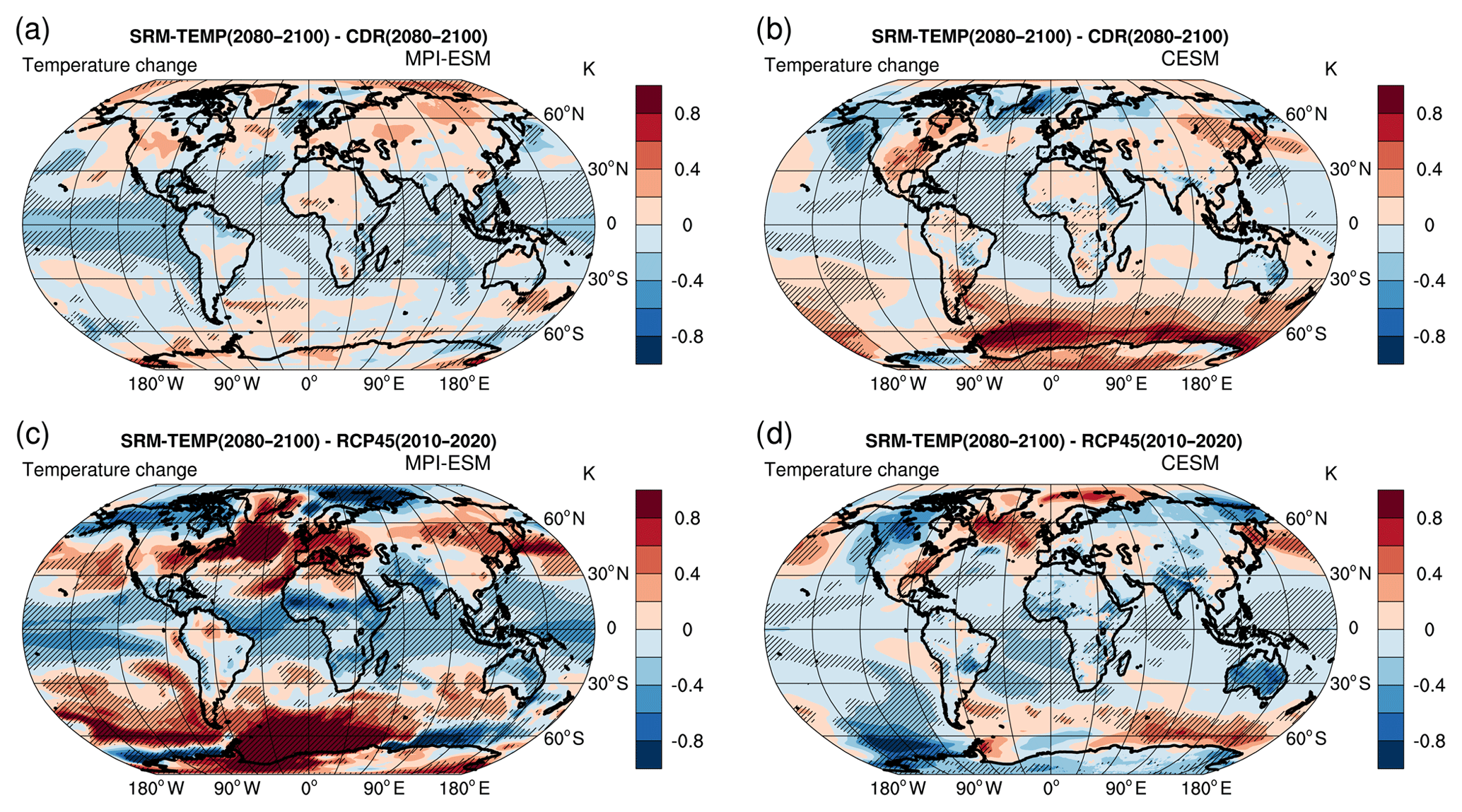
Figure 9Differences in regional temperature patterns between the SRM-TEMP and CDR scenarios for the years 2080–2100 in (a) MPI-ESM and (b) CESM. Also shown are the temperature differences between the SRM-TEMP scenario for the years 2080–2100 and present-day climate (RCP4.5, years 2010–2020) in (c) MPI-ESM and (d) CESM. Hatching indicates regions where the temperature change is statistically significant at the 95 % level, with significance levels estimated using a Student's paired t test (sample of 20 yearly mean values for three ensemble members).
Figure 9c and d compare the SRM-TEMP scenario to present-day climate (2010–2020). In MPI-ESM, the regional SRM-TEMP versus present-day temperature differences were significantly larger than those between SRM-TEMP and CDR at the end of the century. However, this was not the case in the CESM simulations. It should be kept in mind that comparing the years 2080–2100 from the SRM-TEMP scenario with 2010–2020 (as present day) is a somewhat arbitrary choice, and the comparison reflects not only geoengineering impacts but also climate change under RCP4.5. In addition, even though the global mean temperature was similar between these two periods, the climate was relatively stable in 2080–2100 but was warming in 2010–2020. The regional patterns seen in Fig. 9c and d thus depend to a degree on the choice of reference years and not only the impacts of geoengineering.
Regional temperature anomalies for other scenarios are provided in Fig. S6. Overall, RCP4.5 led to larger warming at high latitudes than at low latitudes when compared to CDR for the years 2080–2100. The corresponding regional patterns in SRM-PRECI were similar to those in RCP4.5 but with reduced magnitude. Nevertheless, warming in SRM-PRECI relative to the CDR scenario was statistically significant almost everywhere in both models.
Figure 10 shows the relative precipitation differences between the SRM-PRECI and CDR scenarios in boreal winter (DJF) and summer (JJA) in 2080–2100. Globally, CDR led to 0.5 % more precipitation than SRM-PRECI in both models. However, this precipitation change was not regionally or seasonally homogeneous. A key conclusion is that these changes were rarely statistically significant (hatching in Fig. 10) and that there was often not good agreement between models.

Figure 10Relative change in precipitation between the SRM-PRECI and CDR scenarios for (a) December–January–February and (c) June–July–August in MPI-ESM, along with the corresponding figures for CESM (b, d). Hatching indicates regions where the temperature change is statistically significant at the 95 % level, with significance levels estimated using a Student's paired t test with (sample of 20 yearly mean values for three ensemble members).
Both models did show broadly similar responses over tropical oceans, especially over the eastern Pacific and Atlantic. This was probably caused by an Intertropical Convergence Zone (ITCZ) shift due to the zonal temperature difference between SRM-PRECI and CDR (SRM-PRECI led to more warming in high versus low latitudes compared to CDR). Generally, the responses seen in Fig. 10 were larger in MPI-ESM than in CESM, likely due to the significantly warmer climate in MPI-ESM under SRM-PRECI. Figures S7 and S8 show that when comparing temperature in SRM-PRECI and CDR, simulations with MPI-ESM led to much greater warming in DJF and (especially) JJA over Europe, Australia, and South America when compared to CESM. Figure 10 shows that the corresponding precipitation responses were also significantly different over these areas. Precipitation responses for the other studied scenarios are shown in Figs. S9 and S10. As with the results in Fig. 10, the spatial features of these precipitation responses were rarely statistically significant. To increase confidence in how SRM and CDR would affect regional precipitation distributions, longer simulations or larger ensemble sizes are necessary.
Here, we have studied different scenarios in which global mean warming and precipitation changes are compensated for by solar radiation management (SRM) or carbon dioxide removal (CDR) during the 21st century. We carried out simulations using two Earth system models, MPI-ESM and CESM, with SRM based on stratospheric aerosols first simulated with the aerosol–climate model ECHAM-HAMMOZ. SRM was used for two scenarios in which the magnitude of sulfur injections was controlled to maintain global mean temperature or precipitation at year 2010–2020 levels in the RCP4.5 scenario. Additionally, an idealized CDR scenario (also based on RCP4.5) was performed that included 1 % yr−1 removal of atmospheric CO2. We examined the resulting global mean precipitation changes by dividing the response into temperature-dependent and temperature-independent components. These model-specific components were defined based on a regression method using simulations with fixed climate conditions and that included a constant SRM treatment or an abrupt change in atmospheric CO2 concentrations.
Our work supports prior studies in showing that the ratio of the global precipitation change to the global temperature change for SRM is larger than for an atmospheric CO2 perturbation (e.g. Bala et al., 2008). Thus, less sulfur was needed to compensate for the global mean precipitation change under RCP4.5 than to compensate for the corresponding temperature. Our results showed that maintaining global precipitation at the same level from 2010 to 2100 required a total of 107–113 Tg S with MPI-ESM and 95–114 Tg S with CESM. However, preventing an increase in global mean temperature required 292–318 Tg S with MPI-ESM and 163–199 Tg S with CESM. To give perspective to this, keeping global precipitation at current levels through 2100 would thus require roughly the same amount of sulfur as the estimated surface emissions of China alone between 1996 and 2005 (121 Tg S; Smith et al., 2011; http://sedac.ciesin.columbia.edu/data/set/haso2-anthro-sulfur-dioxide-emissions-1850-2005-v2-86/data-download last access: 9 March 2018). This simultaneously reduced global mean warming by 50 % and 78 % based on the MPI-ESM and CESM simulations, respectively (compared to the 2010–2100 RCP4.5 temperature increase in the absence of SRM).
While completely preventing global mean warming in this century (in RCP4.5) would require much more sulfur than preventing a change in global precipitation, the total sulfur required was comparable to that emitted globally at the surface from anthropogenic sources during the first 5 years of the 21st century (274 Tg S; Smith et al., 2011). However, maintaining a constant global mean temperature in this way led to a significant reduction in global mean precipitation (−1.42 % with MPI-ESM and −0.73 % with CESM) compared to present-day climate. Our component analysis showed that this precipitation decrease was caused by the temperature-independent radiation component resulting from the CO2 increase in the RCP4.5 scenario. Under RCP4.5 without SRM, this component was overridden by the temperature-dependent effect on precipitation from global warming. When this temperature component was compensated for by SRM, the CO2 component remains and global mean precipitation decreases. It should be noted that this is the case for all SRM methods and not only for stratospheric aerosols. SRM itself had only a small temperature-independent fast effect on precipitation.
In the CDR scenario, the annual CO2 increase based on RCP4.5 was counteracted by a 1 % annual removal of the atmospheric CO2 concentration until the year 2070. This was found to slow down warming significantly and to return the global mean temperature to its present-day (2010–2020) value. The atmospheric CO2 budget is currently increasing at roughly 4 Gt C yr−1. In our CDR scenario, 8.7 Gt C yr−1 of CO2 was removed at the year 2020. Our scenario should be considered an idealized high-end CDR scenario, as achieving this high CO2 removal rate in a few years would not be feasible due to technological, economic, social, and political constraints. The results highlight the challenge of substantially slowing global warming and suggest that entirely preventing global mean warming during this century solely via CDR without significant cuts in CO2 emissions is probably not achievable.
Even though global mean temperature at the end of the CDR simulation was the same as at the beginning, global mean precipitation increased (∼0.5 %) in both ESMs. To date, we have not seen as large an increase in global mean precipitation as would be expected only based on the temperature increase (Allan et al., 2014). This is because the fast radiation-driven precipitation effect is largely compensating for the slower temperature-dependent component from warming. However, over time, the temperature component will dominate, and a significant increase in global mean precipitation is expected. If atmospheric CO2 is removed as in the CDR scenario, the temperature component will be prevented from increasing, but simultaneously a positive fast CO2 precipitation component will be induced by the reduction of CO2, increasing global mean precipitation. It is thus difficult to prevent an increase in global mean precipitation via GHG reduction. However, global precipitation changes are also driven by the fast radiative components of aerosols and non-CO2 GHGs, and future precipitation will depend on how these emissions evolve over time.
The RCP4.5 and CDR scenarios led to a similar global mean precipitation response between the two ESMs. However, regression analysis revealed that this was fortuitous. The precipitation response to changing temperature and CO2 concentrations differed between the ESMs, but these differences were masked by offsetting background (BG) effects related to other GHGs and tropospheric aerosols. Large differences in the primary drivers of precipitation change can therefore exist between ESMs even when the ESMs predict similar net changes. A more detailed component analysis, with BG effects separated into relevant subcomponents, is therefore needed. The Precipitation Driver Response Model Intercomparison Project (PDRMIP) may help address this issue (Myhre et al., 2017).
Similar component analyses as done here on the global scale (Sect. 4.2) can in principle be performed regionally. However, for regional analyses (e.g. applying Eq. 2) for a single model grid box, the dry static energy flux divergence of the atmosphere needs to be taken into account (Richardson et al., 2016). This term depends on the neighbouring grid boxes and is not linear or independent from other components. Because of this and natural variability, regression analyses to quantify the fast and slow precipitation components either regionally or for individual grid boxes will be subject to noisier data than in the global case. However, preliminary analyses reveal regions where the approach appears promising, and we therefore recommend further evaluation of this potential in subsequent work.
Overall, this study shows that global mean temperature-independent fast and temperature-dependent slow precipitation responses caused by CDR and SRM can be quantified by the regression method. When these components are known, the global mean precipitation change can be presented as the sum of the temperature-dependent slow component and all fast components. Our results show that the fast responses of CO2 have a major role in the resulting precipitation impacts when CO2-induced global warming is slowed down by geoengineering. If global warming is prevented by stratospheric sulfur injections while the atmospheric CO2 concentration still increases, the global mean precipitation is decreased due to the fast response of increasing atmospheric CO2. On the other hand, less sulfur is required to keep the global mean precipitation stable because the fast precipitation response to increased CO2 is the opposite of the slow precipitation response resulting from a warmer climate. Without SRM, the temperature response overruns the CO2 fast response (as in RCP4.5). Also in our CDR scenario, the global mean precipitation increase was explained by the positive fast precipitation response to reduced CO2. As we showed here, separating precipitation into the fast and slow response is a useful method to analyse differing precipitation responses between different geoengineering techniques. This framework can thus help us to understand and anticipate temperature and precipitation responses on different timescales and under different geoengineering scenarios in which SRM and CDR are potentially used simultaneously. In principle, this method can also be used to study the precipitation response in any scenario if the temperature change and forcing agents are known.
The data from the model simulations and implemented model codes are available from the authors upon request.
The supplement related to this article is available online at: https://doi.org/10.5194/esd-11-415-2020-supplement.
AL designed the research, performed the experiments, carried out the analysis, and prepared the paper. All authors contributed ideas, participated in interpretation and discussion of the results, and contributed to writing the paper.
The authors declare that they have no conflict of interest.
The ECHAM-HAMMOZ model is developed by a consortium composed of ETHZ, Max-Planck Institut für Meteorologie, Forschungszentrum Jülich, the University of Oxford, and the Finnish Meteorological Institute; it is managed by the Center of Climate Systems Modeling (C2SM) at ETHZ.
This research has been supported by the Tiina and Antti Herlin Foundation (grant no. 20150826), the Fonds de Recherche du Québec, – Nature et technologies (grant no. 200414), the Concordia Institute for Water, Energy and Sustainable Systems (CIWESS), and the Academy of Finland (grant no. 308365).
This paper was edited by Valerio Lucarini and reviewed by Tamas Bodai and one anonymous referee.
Allan, R., Liu, C., Zahn, M., Lavers, D., Koukouvagias, E., and Bodas-Salcedo, A.: Physically Consistent Responses of the Global Atmospheric Hydrological Cycle in Models and Observations, Surv. Geophys., 35, 533–552, https://doi.org/10.1007/s10712-012-9213-z, 2014.
Bala, G., Duffy, P. B., and Taylor, K. E.: Impact of geoengineering schemes on the global hydrological cycle, P. Natl. Acad. Sci. USA, 105, 7664–7669, https://doi.org/10.1073/pnas.0711648105, 2008.
Bala, G., Caldeira, K., and Nemani, R.: Fast versus slow response in climate change: implications for the global hydrological cycle, Clim. Dynam., 35, 423–434, https://doi.org/10.1007/s00382-009-0583-y, 2009.
Bergman, T., Kerminen, V.-M., Korhonen, H., Lehtinen, K. J., Makkonen, R., Arola, A., Mielonen, T., Romakkaniemi, S., Kulmala, M., and Kokkola, H.: Evaluation of the sectional aerosol microphysics module SALSA implementation in ECHAM5HAM aerosol-climate model, Geosci. Model Dev., 5, 845–868, https://doi.org/10.5194/gmd-5-845-2012, 2012.
Bódai, T., Lucarini, V., and Lunkeit, F.: Can we use linear response theory to assess geoengineering strategies?, Chaos, 30, 023124, https://doi.org/10.1063/1.5122255, 2020.
Caldeira, K., Govindasamy, B., and Cao, L.: The Science of Geoengineering, Annu. Rev. Earth Planet. Sci., 41, 231–256, https://doi.org/10.1146/annurev-earth-042711-105548, 2013.
Collins, M., Minobe, S., Barreiro, M., Bordoni, S., Kaspi, Y., Kuwano-Yoshida, A., Keenlyside, N., Manzini, E., O'Reilly, C. H., Sutton, R., Xie, S., and Zolina, O.: Challenges and opportunities for improved understanding of regional climate dynamics, Nat. Clim. Change, 8, 101–108, https://doi.org/10.1038/s41558-017-0059-8, 2018.
DeAngelis, A. M., Qu, X., and Hall, A.: Importance of vegetation processes for model spread in the fast precipitation response to CO2 forcing, Geophys. Res. Lett., 43, 12550–12559, https://doi.org/10.1002/2016GL071392, 2016.
Duan, L., Cao, L., Bala, G., and Caldeira, K.: Comparison of the fast and slow climate response to three radiation management geoengineering schemes, J. Geophys. Res.-Atmos., 123, 11980–12001, https://doi.org/10.1029/2018JD029034, 2018
English, J. M., Toon, O. B., and Mills, M. J.: Microphysical simulations of sulfur burdens from stratospheric sulfur geoengineering, Atmos. Chem. Phys., 12, 4775–4793, https://doi.org/10.5194/acp-12-4775-2012, 2012.
Etminan, M., Myhre, G., Highwood, E. J., and Shine, K. P.: Radiative forcing of carbon dioxide, methane, and nitrous oxide: A significant revision of the methane radiative forcing, Geophys. Res. Lett., 43, 12614–12623, https://doi.org/10.1002/2016GL071930, 2016.
Fildier, B. and Collins, W. D.: Origins of climate model discrepancies in atmospheric shortwave absorption and global precipitation changes, Geophys. Res. Lett., 42, 8749–8757, https://doi.org/10.1002/2015GL065931, 2015.
Fläschner, D., Mauritsen, T., and Stevens, B.: Understanding the Intermodel Spread in Global-Mean Hydrological Sensitivity, J. Climate, 29, 801–817, https://doi.org/10.1175/JCLI-D-15-0351.1, 2016.
Frölicher, T. L. and Joos, F.: Reversible and irreversible impacts of greenhouse gas emissions in multi-century projections with the NCAR global coupled carbon cycle-climate model, Clim. Dynam., 35, 1439–1459, https://doi.org/10.1007/s00382-009-0727-0, 2010.
Fuss, S., Lamb, W., Callaghan, M., Hilaire, J., Creutzig, F., Amann, T., and Minx, J.: Negative emissions – Part 2: Costs, potentials and side effects, Environ. Res. Lett., 13, 063002, https://doi.org/10.1088/1748-9326/aabf9f, 2018.
Giorgetta, M., Jungclaus, J., Reick, C. H., Legutke, S., Bader, J., Böttinger, M., Brovkin, V., Crueger, T., Esch, M., Fieg, K., Glushak, K., Gayler, V., Haak, H., Hollweg, H.-D., Ilyina, T., Kinne, S., Kornblueh, L., Matei, D., Mauritsen, T., Mikolajewicz, U., Mueller, W., Notz, D., Pithan, F., Raddatz, T., Rast, S., Redler, R., Roeckner, E., Schmidt, H., Schnur, R., Segschneider, J., Six, K. D., Stockhause, M., Timmreck, C., Wegner, J., Widmann, H., Wieners, K.-H., Claussen, M., Marotzke, J., and Stevens, B.: Climate and carbon cycle changes from 1850 to 2100 in MPI-ESM simulations for the coupled model intercomparison project phase 5, J. Adv. Model. Earth Syst., 5, 572–597, https://doi.org/10.1002/jame.20038, 2013.
GISTEMP Team: GISS Surface Temperature Analysis (GISTEMP), NASA Goddard Institute for Space Studies, available at: https://data.giss.nasa.gov/gistemp/, last access: 3 April 2019.
Gregory, J. M., Ingram, W. J., Palmer, M. A., Jones, G. S., Stott, P. A., Thorpe, R. B., Lowe, J. A., Johns, T. C., and Williams, K. D.: A new method for diagnosing radiative forcing and climate sensitivity, Geophys. Res. Lett., 31, L03205, https://doi.org/10.1029/2003GL018747, 2004.
Heckendorn, P., Weisenstein, D., Fueglistaler, S., Luo, B. P., Rozanov, E., Schraner, M., Thomason, L. W., and Peter, T.: The impact of geoengineering aerosols on stratospheric temperature and ozone, Environ. Res. Lett., 4, 045108, https://doi.org/10.1088/1748-9326/4/4/045108, 2009.
Hienola, A., Partanen, A.-I. Pietikäinen, J., O'Donnel, D., Korhonen, H., Matthews, D., and Laaksonen, A.: The impact of aerosol emissions on the 1.5 ∘C pathways, Environ. Res. Lett., 13, 04401, https://doi.org/10.1088/1748-9326/aab1b2, 2018.
Hurrell, J. W., Holland, M. M., Gent, P. R., Ghan, S., Kay, J. E., Kushner, P. J., Lamarque, J.-F., Large, W. G., Lawrence, D., Lindsay, K., Lipscomb, W. H., Long, M. C., Mahowald, N., Marsh, D. R., Neale, R. B., Rasch, P., Vavrus, S., Vertenstein, M., Bader, D., Collins, W. D., Hack, J. J., Kiehl, J., and Marshall, S.: The Community Earth System Model: a framework for collaborative research, B. Am. Meteorol. Soc., 94, 1339–1360, https://doi.org/10.1175/BAMS-D-12-00121.1, 2013.
Ilyina, T., Six, K. D., Segschneider, J., Maier-Reimer, E., Li, H., and Nunez-Riboni, I.: Global ocean biogeochemistry model HAMOCC: Model architecture and performance as component of the MPI-Earth System Model in different CMIP5 experimental realizations, J. Adv. Model. Earth Syst., 5, 287–315, https://doi.org/10.1029/2012MS000178, 2013.
IPCC: Climate Change 2014: Synthesis Report, in: Contribution of Working Groups I, II and III to the Fifth Assessment Report of the Intergovernmental Panel on Climate Change, edited by: Core Writing Team, Pachauri, R. K., and Meyer, L. A., IPCC, Geneva, Switzerland, 151 pp., 2014.
IPCC: Global Warming of 1.5 ∘C, in: An IPCC Special Report on the impacts of global warming of 1.5 ∘C above pre-industrial levels and related global greenhouse gas emission pathways, in the context of strengthening the global response to the threat of climate change, sustainable development, and efforts to eradicate poverty, edited by: Masson-Delmotte, V., Zhai, P., Pörtner, H.-O., Roberts, D., Skea, J., Shukla, P. R., Pirani, A., Moufouma-Okia, W., Péan, C., Pidcock, R., Connors, S., Matthews, J. B. R., Chen, Y., Zhou, X., Gomis, M. I., Lonnoy, E., Maycock, T., Tignor, M., and Waterfield, T., in press, 2018.
Jungclaus, J. H., Fischer, N., Haak, H., Lohmann, K., Marotzke, J., Matei, D., Mikolajewicz, U., Notz, D., and von Storch, J.-S.: Characteristics of the ocean simulations in MPIOM, the ocean component of the MPI Earth System Model, J. Adv. Model. Earth Syst., 5, 422–446, https://doi.org/10.1002/jame.20023, 2013.
Kinne, S., O'Donnell, D., Stier, P., Kloster, S., Zhang, K., Schmidt, H., Rast, S., Giorgetta, M., Eck, T. F., and Stevens, B.: MAC-v1: A new global aerosol climatology for climate studies, J. Adv. Model. Earth Syst., 5, 704–740, https://doi.org/10.1002/jame.20035, 2013.
Knutti, R. and Sedláček, J.: Robustness and uncertainties in the new CMIP5 climate model projections, Nat. Clim. Change, 3, 369–373, https://doi.org/10.1038/nclimate1716, 2012.
Kokkola, H., Korhonen, H., Lehtinen, K. E. J., Makkonen, R., Asmi, A., Järvenoja, S., Anttila, T., Partanen, A.-I., Kulmala, M., Järvinen, H., Laaksonen, A., and Kerminen, V.-M.: SALSA – a Sectional Aerosol module for Large Scale Applications, Atmos. Chem. Phys., 8, 2469–2483, https://doi.org/10.5194/acp-8-2469-2008, 2008.
Kokkola, H., Kühn, T., Laakso, A., Bergman, T., Lehtinen, K. E. J., Mielonen, T., Arola, A., Stadtler, S., Korhonen, H., Ferrachat, S., Lohmann, U., Neubauer, D., Tegen, I., Siegenthaler-Le Drian, C., Schultz, M. G., Bey, I., Stier, P., Daskalakis, N., Heald, C. L., and Romakkaniemi, S.: SALSA2.0: The sectional aerosol module of the aerosol–chemistry–climate model ECHAM6.3.0-HAM2.3-MOZ1.0, Geosci. Model Dev., 11, 3833–3863, https://doi.org/10.5194/gmd-11-3833-2018, 2018.
Koll, D. D. P. and Cronin, T. W.: Earth's outgoing longwave radiation linear due to H2O greenhouse effect, P. Natl. Acad. Sci. USA, 115, 10293–10298, https://doi.org/10.1073/pnas.1809868115, 2018.
Kravitz, B., Caldeira, K., Boucher, O., Robock, A., Rasch, P. J., Alterskjær, K., Karam, D., B., Cole, J. N. S., Curry, C. L., Haywood, J. M., Irvine, P. J., Ji, D., Jones, A., Kristjánsson, J. E., Lunt, D. J., Moore, J. C., Niemeier, U., Schmidt, H., Schulz, M., Singh, B., Tilmes, S., Watanabe, S., Yang, S., and Yoon, J.-H.: Climate model response from the Geoengineering Model Intercomparison Project (GeoMIP), J. Geophys. Res.-Atmos., 118, 8320–8332, https://doi.org/10.1002/jgrd.50646, 2013.
Kvalevåg, M. M., Samset, B. H., and Myhre, G.: Hydrological sensitivity to greenhouse gases and aerosols in a global climate model, Geophys. Res. Lett., 40, 1432–1438, https://doi.org/10.1002/grl.50318, 2013.
Laakso, A., Kokkola, H., Partanen, A.-I., Niemeier, U., Timmreck, C., Lehtinen, K. E. J., Hakkarainen, H., and Korhonen, H.: Radiative and climate impacts of a large volcanic eruption during stratospheric sulfur geoengineering, Atmos. Chem. Phys., 16, 305–323, https://doi.org/10.5194/acp-16-305-2016, 2016.
Laakso, A., Korhonen, H., Romakkaniemi, S., and Kokkola, H.: Radiative and climate effects of stratospheric sulfur geoengineering using seasonally varying injection areas, Atmos. Chem. Phys., 17, 6957–6974, https://doi.org/10.5194/acp-17-6957-2017, 2017.
Lausier, A. M. and Jain S.: Overlooked Trends in Observed Global Annual Precipitation Reveal Underestimated Risks, Scient. Rep., 8, 16746, https://doi.org/10.1038/s41598-018-34993-5, 2018.
Lenssen, N., Schmidt, G., Hansen, J., Menne, M., Persin, A., Ruedy, R., and Zyss, D.: Improvements in the GISTEMP uncertainty model, J. Geophys. Res.-Atmos., 124, 6307–6326, https://doi.org/10.1029/2018JD029522, 2019.
Li, C., McLinden, C., Fioletov, V., Krotkov, N., Carn, S., Joiner, J., Streets, D., He, H., Ren, X., Li, Z., and Dickerson, R. R.: India is overtaking China as the World's largest emitter of anthropogenic sulfur dioxide, Sci. Rep., 7, 14304, https://doi.org/10.1038/s41598-017-14639-8, 2017.
Liu, W., Sun, F., Lim, W. H., Zhang, J., Wang, H., Shiogama, H., and Zhang, Y.: Global drought and severe drought-affected populations in 1.5 and 2 ∘C warmer worlds, Earth Syst. Dynam., 9, 267–283, https://doi.org/10.5194/esd-9-267-2018, 2018.
Luderer, G., Vrontisi, Z., Bertram, C., Edelenbosch, O., Pietzcker, R., Rogelj, J., and Kriegler, E.: Residual fossil CO2 emissions in 1.5–2 ∘C pathways, Nat. Clim. Change, 8, 626–633, https://doi.org/10.1038/s41558-018-0198-6, 2018.
Marvel, K., Schmidt, G. A., Shindell, D., Bonfils, C., LeGrande, A. N., Nazarenko, L., and Tsigaridis, K.: Do responses to different anthropogenic forcings add linearly in climate models?, Environ. Res. Lett., 10, 104010, https://doi.org/10.1088/1748-9326/10/10/104010, 2015.
Millar, R., Fuglestvedt, J., Friedlingstein, P., Rogelj, J., Grubb, M., Matthews, H., and Allen, M.: Emission budgets and pathways consistent with limiting warming to 1.5 ∘C, Nat. Geosci., 10, 741–747, https://doi.org/10.1038/ngeo3031, 2017.
Moss, R. H., Edmonds, J. A., Hibbard, K. A., Manning, M. R., Rose, S. K., van Vuuren, D. P., Carter, T. R., Emori, S., Kainuma, M., Kram, T., Meehl, G. A., Mitchell, J. F. B., Nakicenovic, N., Riahi, K., Smith, S. J., Stouffer, R. J., Thomson, A. M., Weyant, J. P., and Wilbanks, T. J.: The next generation of scenarios for climate change research and assessment, Nature, 463, 747–756, https://doi.org/10.1038/nature08823, 2010.
Myhre, G., Forster, P. M., Samset, B. H., Hodnebrog, Ø., Sillmann, J., Aalbergsjø, S. G., Andrews, T., Boucher, O., Faluvegi, G., Fläschner, D., Iversen, T., Kasoar, M., Kharin, V., Kirkevåg, A., Lamarque, J., Olivié, D., Richardson, T. B., Shindell, D., Shine, K. P., Stjern, C. W., Takemura, T., Voulgarakis, A., and Zwiers, F.: PDRMIP: A Precipitation Driver and Response Model Intercomparison Project – Protocol and Preliminary Results, B. Am. Meteorol. Soc., 98, 1185–1198, https://doi.org/10.1175/BAMS-D-16-0019.1, 2017.
Niemeier, U. and Timmreck, C.: What is the limit of climate engineering by stratospheric injection of SO2?, Atmos. Chem. Phys., 15, 9129–9141, https://doi.org/10.5194/acp-15-9129-2015, 2015.
Reick, C., Raddatz, T. V., Brovkin, V., and Gayler, V.: The representation of natural and anthropogenic land cover change in MPI-ESM, J. Adv. Model. Earth Syst., 5, 459–482, https://doi.org/10.1002/jame.20022, 2013.
Richardson, T.B., Forster, P. M., Andrews, T., and Parker, D. J.: Understanding the Rapid Precipitation Response to CO2 and Aerosol Forcing on a Regional Scale, J. Climate, 29, 583–594, https://doi.org/10.1175/JCLI-D-15-0174.1, 2016.
Robock, A., Marquardt, A., Kravitz, B., and Stenchikov, G.: Benefits, risks, and costs of stratospheric geoengineering, Geophys. Res. Lett., 36, L19703, https://doi.org/10.1029/2009GL039209, 2009.
Rogelj, J., Shindell, D., Jiang, K., Fifita, S., Forster, P., Ginzburg, V., Handa, C., Kheshgi, H., Kobayashi, S., Kriegler, E., Mundaca, L., Séférian, R., and Vilariño, M. V.: Mitigation pathways compatible with 1.5 ∘C in the context of sustainable development, in: Global warming of 1.5 ∘C. An IPCC Special Report on the impacts of global warming of 1.5 ∘C above pre-industrial levels and related global greenhouse gas emission pathways, in the context of strengthening the global response to the threat of climate change, sustainable development, and efforts to eradicate poverty, edited by: Masson-Delmotte, V., Zhai, P., Pörtner, H. O., Roberts, D., Skea, J., Shukla, P. R., Pirani, A., Moufouma-Okia, W., Péan, C., Pidcock, R., Connors, S., Matthews, J. B. R., Chen, Y., Zhou, X., Gomis, M. I., Lonnoy, E., Maycock, T., Tignor, M., and Waterfield, T., in press, 2018.
Royal Society: Geoengineering the climate – Science, governance and uncertainty, RS Policy document 10/09, London, 2009.
Samset, B. H., Myhre, G., Forster, P. M., Hodnebrog, Ø., Andrews, T., Faluvegi, G., Fläschner, D., Kasoar, M., Kharin, V., Kirkevåg, A., Lamarque, J.-F., Olivié, D., Richardson, T., Shindell, D., Shine, K. P., Takemura, T., and Voulgarakis, A.: Fast and slow precipitation responses to individual climate forcers: A PDRMIP multimodel study, Geophys. Res. Lett., 43, 2782–2791, https://doi.org/10.1002/2016GL068064, 2016.
Schleussner, C.-F., Lissner, T. K., Fischer, E. M., Wohland, J., Perrette, M., Golly, A., Rogelj, J., Childers, K., Schewe, J., Frieler, K., Mengel, M., Hare, W., and Schaeffer, M.: Differential climate impacts for policy-relevant limits to global warming: the case of 1.5 ∘C and 2 ∘C, Earth Syst. Dynam., 7, 327–351, https://doi.org/10.5194/esd-7-327-2016, 2016.
Seneviratne, S., Rogelj, J., Séférian, R., Wartenburger, R., Allen, M., Cain, M., and Warren, R.: The many possible climates from the Paris Agreement's aim of 1.5 ∘C warming, Nature, 558, 41–49, https://doi.org/10.1038/s41586-018-0181-4, 2018.
Smith, S. J., van Aardenne, J., Klimont, Z., Andres, R. J., Volke, A., and Delgado Arias, S.: Anthropogenic sulfur dioxide emissions: 1850–2005, Atmos. Chem. Phys., 11, 1101–1116, https://doi.org/10.5194/acp-11-1101-2011, 2011.
Stevens, B., Giorgetta, M., Esch, M., Mauritsen, T., Crueger, T., Rast, S., Salzmann, M., Schmidt, H., Bader, J., Block, K., Brokopf, R., Fast, I., Kinne, S., Kornblueh, L., Lohmann, U., Pincus, R., Reichler, T., and Roeckner, E.: The atmospheric component of the MPI-M Earth System Model: ECHAM6, J. Adv. Model. Earth Syst., 5, 1–27, https://doi.org/10.1002/jame.20015, 2013.
Thomson, A., Calvin, K., Smith, S., Kyle, G., Volke, A., Patel, P., and Edmonds, J.: RCP4.5: a pathway for stabilization of radiative forcing by 2100, Climatic Change, 109, 77, https://doi.org/10.1007/s10584-011-0151-4, 2011.
Tokarska, K. and Zickfeld, K.: The effectiveness of net negative carbon dioxide emissions in reversing anthropogenic climate change, Environ. Res. Lett., 10, 094013, https://doi.org/10.1088/1748-9326/10/9/094013, 2015.
UNFCCC: Adoption of the Paris Agreement FCCC/CP/2015/L.9/Rev. 1, available at: http://unfccc.int/resource/docs/2015/cop21/eng/l09r01.pdf (last access: 7 January 2019), 2015.
van Vuuren, D. P., den Elzen, M., Lucas, P., Eickhout, B., Strengers, B., van Ruijven, B., Wonink, S., and van Houdt, R.: Stabilizing greenhouse gas concentrations at low levels: an assessment of reduction strategies and costs, Climatic Change, 81, 119–159, https://doi.org/10.1007/s10584-006-9172-9, 2007.
van Vuuren, D. P., Edmonds, J., Kainuma, M., Riahi, K., Thomson, A., Hibbard, K., Hurtt, G. C., Kram, T., Krey, V., Lamarque, J.-F., Masui, T., Meinshausen, M., Nakicenovic, N., Smith, S. J., and Rose, S. K.: The representative concentration pathways: an overview, Climatic Change, 109, 5–31, https://doi.org/10.1007/s10584-011-0148-z, 2011.
Wu, P., Ridley, J., Pardaens, A., Levine, R., and Lowe, J.: The reversibility of CO2 induced climate change, Clim. Dynam., 45, 745–754, https://doi.org/10.1007/s00382-014-2302-6, 2015.
Zhang, K., O'Donnell, D., Kazil, J., Stier, P., Kinne, S., Lohmann, U., Ferrachat, S., Croft, B., Quaas, J., Wan, H., Rast, S., and Feichter, J.: The global aerosol-climate model ECHAM-HAM, version 2: sensitivity to improvements in process representations, Atmos. Chem. Phys., 12, 8911–8949, https://doi.org/10.5194/acp-12-8911-2012, 2012.
- Abstract
- Introduction
- Methods
- Fast and slow components of radiation and precipitation
- Results from simulated scenarios
- Sulfur injections
- Regional climate responses
- Discussion and conclusions
- Code and data availability
- Author contributions
- Competing interests
- Acknowledgements
- Financial support
- Review statement
- References
- Supplement